Investigating mixed-integer programming approaches for the $p$-$\alpha$-closest-center problem

Abstract

In this work, we introduce and study the $p$-$\alpha$-closest-center problem ($p\alpha$CCP), which is a generalization of the $p$-second-center problem, a recently emerged variant of the classical (discrete) $p$-center problem. In the $p\alpha$CCP, we are given a discrete set of customers, a discrete set of potential facility locations, distances between each customer and potential facility location as well as two integers $p$ and $\alpha$. The goal is to open facilities at $p$ of the potential facility locations, such that the maximum $\alpha$-distance between each customer and the open facilities is minimized. The $\alpha$-distance of a customer is defined as the sum of distances from the customer to its $\alpha$ closest open facilities. If $\alpha$ is set to one, the $p\alpha$CCP is the $p$-center problem, and for $\alpha$ being two, the $p$-second-center problem is obtained, for which the only existing algorithm in literature is a variable neighborhood search (VNS).

We first prove relationships between the optimal objective function values for different variants of the $p$-center problem to set the $p\alpha$CCP in context with existing problems. We then present four mixed-integer programming (MIP) formulations for the $p\alpha$CCP and strengthen them by adding valid and optimality-preserving inequalities. We also conduct a polyhedral study to prove relationships between the linear programming relaxations of our MIP formulations. Moreover, we present iterative procedures for lifting some valid inequalities to improve initial lower bounds on the optimal objective function value of the $p\alpha$CCP and characterize the best lower bounds obtainable by this iterative lifting approach.

Based on our theoretical findings, we develop a branch-and-cut algorithm (B&C) to solve the $p\alpha$CCP exactly. We improve its performance by a starting and a primal heuristic, variable fixings and separating inequalities. In our computational study, we investigate the effect of the various ingredients of our B&C on benchmark instances from related literature. Our B&C is able to prove optimality for 17 of the 40 instances from the work on the VNS heuristic.

1 Introduction

The (discrete) $p$-center problem ($p$CP) is a fundamental problem in location science (see, e.g., the book-chapter Çalık et al. (2019)) that was first introduced in Hakimi (1965). In the $p$CP, we are given a set of customer locations $I$, a set of potential facility locations $J$, an integer $p<|J|$ and distances $d_{ij}\geq 0$ between each customer location $i\in I$ and potential facility location $j\in J$. The goal is to open $p$ facilities in such a way that the maximum distance of any customer location to its closest open facility is minimized. The problem is NP-hard as proven by Kariv and Hakimi (1979) and one of its main application areas is the placement of emergency services and relief actions in humanitarian crisis as described in Jia et al. (2007); Çalık and Tansel (2013) and Lu and Sheu (2013). Motivated by the fact that in such settings, facilities may fail for various reasons, different variants of the $p$CP such as the $\alpha$-neighbor-$p$-center problem ($\alpha$N$p$CP) defined in Krumke (1995) and the $p$-next-center problem ($p$NCP) introduced by Albareda-Sambola et al. (2015) have emerged to deal better with the issue of failing facilities. Another variant motivated by this issue is the $p$-second-center problem ($p$SCP). It was first mentioned in López-Sánchez et al. (2019) and only recently studied in Ristić et al. (2023b), where the authors present a heuristic solution approach. At the end of their work, they also propose that a generalization of this problem should be studied, which they call the $p$-$\alpha$-closest-center problem. In this paper we follow this suggestion and start by giving its definition.

Definition 1 (The $p$-$\alpha$-closest-center problem).

Let $I$ be a set of customer locations and $J$ be a set of potential facility locations with distances $d_{ij}\geq 0$ between customer locations $i\in I$ and potential facility locations $j\in J$. Let $n=|I|$, $m=|J|$ and let $\alpha$ and $p$ be two integers with $1\leq\alpha\leq p<m$. A feasible solution to the $p$-$\alpha$-closest-center problem ($p\alpha$CCP) consists of a subset $P\subseteq J$ of open facilities with $|P|=p$. Given a feasible solution $P$ and a customer location $i\in I$, the $\alpha$-distance $d_{\alpha}(P,i)$ is defined as

$$d_{\alpha}(P,i)=\min_{\begin{subarray}{c}A\subseteq P\\ |A|=\alpha\end{subarray}}\sum_{j\in A}d_{ij}.$$

The objective function value $f_{\alpha}(P)$ of a feasible solution $P$ is defined as

$$f_{\alpha}(P)=\max_{i\in I}d_{\alpha}(P,i).$$

Using these definitions, the $p\alpha$CCP can be formulated as

$$\min_{\begin{subarray}{c}P\subseteq J\\ |P|=p\end{subarray}}f_{\alpha}(P).$$

For the sake of brevity, we also write customers instead of customer locations and facilities instead of potential facility locations in the remainder of this paper. Note, that for $\alpha=1$, the $p\alpha$CCP is exactly the $p$CP, and for $\alpha=2$ we obtain the $p$SCP. The motivation behind the $p\alpha$CCP is that in case of failing facilities, the closest open facility for some customer in an optimal solution of the $p$CP may fail, and thus this customer must travel to another open facility. As the $p$CP only considers the closest open facility for each customer in the objective function, this other open facility may be far from it. The $p\alpha$CCP deals with this issue by considering the distance to $\alpha$ facilities in the objective function by minimizing the average distance from a customer to its $\alpha$ closest open facilities. Therefore, it minimizes the average distance this customer needs to travel if its $\beta$ closest open facilities fail over all $\beta\in\{0,1,\ldots,\alpha-1\}$. As our main contribution in this paper, we investigate the $p\alpha$CCP both from a theoretical and a practical side.

However, we also compare the $p\alpha$CCP to other variants of the $p$CP to set it in context. Thus, we next discuss some of them in more detail. The $\alpha$N$p$CP is defined as

$$\min_{\begin{subarray}{c}P\subseteq V\\ |P|=p\end{subarray}}\max_{i\in V\setminus P}\min_{\begin{subarray}{c}A\subseteq P\\ |A|=\alpha\end{subarray}}\max_{j\in A}d_{ij}.$$

It aims to open a set of facilities $P$ such that the maximum distance between a customer and its $\alpha$-closest open facility is minimized. The idea behind it is that the $\alpha-1$ closest facilities to a customer may fail. Then, the customer needs to travel to the $\alpha$-closest facility, which therefore should not be too far away. We note that unlike the setting in the $p\alpha$CCP, the $\alpha$N$p$CP has a single set $V$ of locations as input. The set of customer locations is then defined as the set of elements where no facility is opened, i.e., $I=V\setminus P$ depends on the feasible solution $P$.

A different approach is modeled by the $p$NCP. The idea is that if the closest open facility to a customer has failed, the customer may only notice this when she has arrived at the failed facility. In this case, it can be useful if the next open facility is near the facility the customer has just arrived. Therefore, the $p$NCP aims to minimize the maximum sum of distances from a customer location to its closest open facility and from this closest open facility to the closest open alternative facility. It can be formally defined as

$$\min_{\begin{subarray}{c}P\subseteq V\\ |P|=p\end{subarray}}\max_{i\in I}\left(\min_{j\in P}d_{ij}+\min_{\begin{subarray}{c}k\in P\\ j^{\prime}\in\arg\min_{j\in P}d_{ij}\\ k\neq j^{\prime}\end{subarray}}d_{j^{\prime}k}\right).$$

Note, that the $p$NCP does not require the $\alpha$ parameter, but compared to the $p\alpha$CCP it additionally needs distances between potential facility locations as input.

For the remainder of this paper, we use the following notation. For a problem, a mixed-integer program (MIP) or a linear program (LP) $F$, we denote the optimal objective function value of $F$ by $\nu(F)$. Moreover, we denote the LP-relaxation of a MIP ($F$) by ($F$-R). Additionally, let $\mathcal{J}^{\alpha}=\{A\subseteq J:|A|=\alpha\}$ be the set of all subsets of $J$ of cardinality $\alpha$. Then, we define $d_{iA}=\sum_{j\in A}d_{ij}$ and $d_{iA}^{\max}=\max\{d_{ij}:j\in A\}$ for all $i\in I$ and $A\in\mathcal{J}^{\alpha}$. Furthermore, let $D^{\alpha}=\{d_{iA}:i\in I,A\in\mathcal{J}^{\alpha}\}$ be the set of all possible $\alpha$-distances.

1.1 Contribution and outline

This work formally defines and studies the $p\alpha$CCP. We embed this new problem into the context of existing $p$CP variants by proving relationships between their optimal objective function values. We further introduce four different mixed-integer programming (MIP) formulations of the $p\alpha$CCP, which are the very first for this problem and also for the $p$SCP. We present several valid inequalities and so-called optimality-preserving inequalities, i.e., inequalities that may cut off feasible solutions, but that do not change the optimal objective function value. We conduct a polyhedral study on all formulations and study their semi-relaxations, in which only some of the binary variables are relaxed.

For three of our MIP formulations, we also present valid inequalities that incorporate a lower bound on the optimal objective function of the $p\alpha$CCP, i.e., lifted inequalities. Adding these inequalities iteratively yields a procedure to improve such lower bounds similar to the approaches in Gaar and Sinnl (2022) and Gaar and Sinnl (2023) for the $p$CP and the $\alpha$N$p$CP, respectively. We prove convergence of this iterative procedure and give a characterization of the best obtainable lower bound as a solution of a set cover problem variant for some of the MIP formulations. Moreover, we compare the three best obtainable lower bounds in this way with each other and prove that two of them coincide.

We develop a branch-and-cut algorithm based on our theoretical results, which is the first algorithm to solve the $p\alpha$CCP and the $p$SCP exactly. We introduce a starting and a primal heuristic as well as variable fixing procedures and study their effects on the algorithms performance. Our computational tests are made on 93 different instances from the literature, of which we could solve 52 instances to optimality. We compare our results to the heuristic of Ristić et al. (2023b) and prove optimality of their solutions for 17 instances.

In the remainder of this section we provide an overview of related work. In Section 2, we discuss the relationships between several $p$CP variants, including the $\alpha$N$p$CP, the $p$NCP and the $p\alpha$CCP. Section 3 contains our four MIP formulations of the $p\alpha$CCP together with strengthening inequalities and in Section 4, a polyhedral study is conducted. Section 5 contains the lifted inequalities and the iterative procedure for our third and fourth MIP formulation. Section 6 describes a similar approach for our first MIP formulation, which is much more involved for this formulation compared to that for the third and fourth formulation. In Section 7, we present our branch-and-cut algorithm based on our first MIP formulation and some implementation details. The results of our computational experiments are discussed in Section 8 and Section 9 provides closing remarks.

1.2 Literature review

López-Sánchez et al. (2019) are the first to mention the $p$SCP as a possible new $p$CP variant. However, they do not investigate it. This was only recently done by Ristić et al. (2023b). These authors propose a variable neighborhood search (VNS) to heuristically solve the $p$SCP. They also mention the NP-hardness of the problem as it is a generalization of the NP-hard $p$CP. Aside from López-Sánchez et al. (2019) and Ristić et al. (2023b) we are not aware of any other work considering the $p$SCP. For the related problems mentioned in the introduction, there is various existing research as we discuss next.

The $p$-center problem

The $p$CP itself was already introduced by Hakimi (1965) and since its introduction there has been an enormous amount of work on it, both from the exact as well as from the (meta-)heuristic side. As we are concerned with the design of exact solution algorithms in our work, we focus this overview on exact methods and refer to Garcia-Diaz et al. (2019) for heuristics and approximation algorithms.

Minieka (1970) presents the first exact algorithm for the $p$CP. This approach uses the connection of the $p$CP to the set cover problem (SCP), and aims to identify a set of open facilities of minimum cardinality such that every customer demand point is within a given radius of at least one open facility. Consequently, the $p$CP can be solved in an iterative fashion by solving SCPs. Many follow-up works such as Garfinkel et al. (1977); Ilhan and Pinar (2001); Ilhan et al. (2002); Caruso et al. (2003); Al-Khedhairi and Salhi (2005); Chen and Chen (2009) and Contardo et al. (2019) exist.

There are also various MIP formulations for solving the $p$CP to proven optimality. The classical textbook formulation of the $p$CP (see, e.g., Daskin (2013)) uses two sets of variables, namely facility opening variables and assignment variables, and its linear programming (LP)-relaxation is known to have bad bounds as shown for example in Snyder and Shen (2011). Elloumi et al. (2004) present an alternative MIP formulation, which was later simplified in Ales and Elloumi (2018). They show that the LP-relaxation of their formulation can give better bounds compared to the relaxation of the classical formulation. In Çalık and Tansel (2013) another MIP formulation of the $p$CP is developed and the authors prove that its LP-relaxation gives the same bounds as the LP-relaxation of the formulation of Elloumi et al. (2004). In Gaar and Sinnl (2022), a further MIP formulation is obtained by projecting out the assignment variables from the classical formulation, following the Benders approach of Fischetti et al. (2017) for the uncapacitated facility location problem. Moreover, the authors also present an iterative lifting scheme for the inequalities in the new formulation, which, given a lower bound on the optimal objective function value of the $p$CP, potentially improves this lower bound. They prove that the best lower bounds obtainable by this procedure are the same bounds that are obtained by a semi-relaxation of Elloumi et al. (2004).

The $\alpha$-neighbor-$p$-center problem

The $\alpha$N$p$CP was first introduced and studied by the approximation-algorithms community in Krumke (1995); Chaudhuri et al. (1998) and Khuller et al. (2000). In the 2020s, various heuristic works on the problem appeared, namely a greedy randomized adaptive search procedure (GRASP) proposed by Sánchez-Oro et al. (2022), a local search by Mousavi (2023) and a parallel VNS by Chagas et al. (2024). Moreover, Gaar and Sinnl (2023) introduce two MIP formulations of the problem, one based on the classical textbook formulation of the $p$CP and one based on the formulation of Ales and Elloumi (2018) of the $p$CP. For the first formulation, they present valid inequalities using the lower bounds from the LP-relaxation and how these inequalities can be used in an iterative lifting-scheme akin to their approach for the $p$CP in Gaar and Sinnl (2022). For the second formulation, they present an iterative variable fixing scheme based on lower bounds from the LP-relaxation.

As described above, in the $\alpha$N$p$CP, we are given one set of locations, and for a given solution the customer locations are defined as the locations where no facility is opened. However, there is some literature on a variant in which all locations are customer locations. This variant is referred to as the $\alpha$-all-neighbors-$p$-center problem in Khuller et al. (2000) and the fault-tolerant-$p$-center problem in Elloumi et al. (2004).

The $p$-next-center problem

Albareda-Sambola et al. (2015) were the first to introduce the $p$NCP. They prove the NP-hardness of this problem and propose three MIP formulations, which are based on two-index, three-index and covering variables. Furthermore, they compare the performance of those formulations when given to an off-the-shelf MIP solver. The first heuristics for the $p$NCP were proposed by López-Sánchez et al. (2019). They develop a VNS and a GRASP and test a hybridized algorithm as well. Later, Londe et al. (2021) propose an evolutionary algorithm for the $p$NCP and Ristić et al. (2023a) present a different VNS heuristic that is based on the VNS of Mladenović et al. (2003) for the $p$CP.

2 Relationships between $p$CP variants

It becomes clear from the introduction that the described $p$CP variants are all closely related. In this section, we study these relationships in more detail and prove some lower and upper bounds on the optimal objective function value of one $p$CP variant by the one of another $p$CP variant.

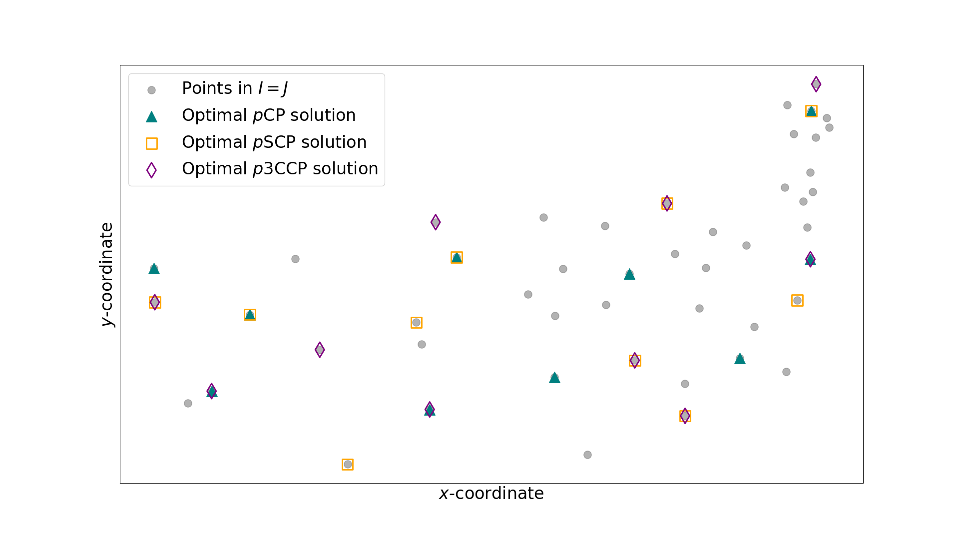
We start by showing an example of optimal solutions for the $p\alpha$CCP for different values of $\alpha$. We consider the instance att48 of the TSPlib instance set from Reinelt (1991) with $I=J$. The distances in this instance are defined as the Euclidean distances between the points in $I=J$, which are given as coordinates in the two-dimensional plane. In Figure 1, we depict an optimal solution of the $p\alpha$CCP with $p=10$ and $\alpha\in\{1,2,3\}$, i.e., for the $p$CP, the $p$SCP and the $p$$3$CCP. For this instance, all obtained optimal solutions differ. The corresponding optimal objective function values are 1203.18, 2827.72 and 4895.52, respectively. For a smaller example showing different optimal solutions for the $p$CP, the $p$SCP and the $p$NCP, we refer to Ristić et al. (2023b).

Figure 1: The locations of the tsplib instance att48 with optimal solutions for the $p$CP, the $p$SCP and the $p$3CCP with $p=10$

Rather than considering optimal solutions, we might also study optimal objective function values. The following theorem provides more detailed information about the relationships between the optimal objective function values of the $p$CP, the $\alpha$N$p$CP, the $p$NCP and the $p\alpha$CCP. Since the $\alpha$N$p$CP is only defined for a single set representing customer locations and potential facility locations at the same time, and because for the $p$NCP we need distances between all pairs of potential facility locations in $J$, we here assume $I=J$ and denote the set by $V$.

Theorem 2.

Let $V=I=J$ be the set of customer and potential facility locations, let $p<|V|$ be an integer and let $d_{ij}\geq 0$ be the distance between two locations $i,j\in V$. Then, the following statements are true:

$$1.\quad \nu(\text{$p$CP}) \leq\nu(\text{$p$NCP})$$

$$2. \nu(\text{$p$CP}) \leq\nu(\text{$\alpha$N$p$CP})\qquad \textrm{for all }\alpha\leq p\textrm{ if }d_{ii}=0\textrm{ for all }i\in V$$

$$3. \nu(\text{$\alpha$N$p$CP}) \leq\nu(\text{$p\alpha$CCP}) \textrm{for all }\alpha\leq p$$

$$4. \nu(\text{$\alpha$N$p$CP}) \leq\nu(\text{$\beta$N$p$CP}) \textrm{for all }\alpha\leq\beta\leq p$$

$$5. \nu(\text{$p\alpha$CCP}) \leq\nu(\text{$p$$\beta$CCP}) \textrm{for all }\alpha\leq\beta\leq p$$

$$6. \nu(\text{2N$p$CP}) \leq\nu(\text{$p$NCP})$$ if the distances satisfy the triangle

$$\qquad\text{inequalities $d_{ij}\leq d_{ik}+d_{kj}$ for all $i,j,k\in V$}.$$

Proof.

1. Let $P^{*}$ be an optimal solution of the $p$NCP. Then,

   $$\nu(\text{$p$CP}) =\min_{\begin{subarray}{c}P\subseteq V\\ |P|=p\end{subarray}}\ \max_{i\in V}\ \min_{j\in P}\ d_{ij}\leq\max_{i\in V}\ \min_{j\in P^{*}}\ d_{ij}=\max_{i\in V}\ (\min_{j\in P^{*}}\ d_{ij}+0)$$

   $$\leq\ \max_{i\in V}\left(\min_{j\in P^{*}}\ d_{ij}+\min_{\begin{subarray}{c}k\in P^{*}\\ j^{\prime}\in\arg\min_{j\in P^{*}}d_{ij},\\ k\neq j^{\prime}\end{subarray}}\ d_{j^{\prime}k}\right)=\nu(\text{$p$NCP}).$$

2. Let $P^{*}$ be an optimal solution of the $\alpha$N$p$CP. Then,

   $$\nu(\text{$p$CP}) =\min_{\begin{subarray}{c}P\subseteq V\\ |P|=p\end{subarray}}\max_{i\in V}\min_{j\in P}d_{ij}\leq\max_{i\in V}\min_{j\in P^{*}}d_{ij}=\max_{i\in V\setminus P^{*}}\min_{j\in P^{*}}d_{ij}$$

   $$=\max_{i\in V\setminus P^{*}}\min_{\begin{subarray}{c}A\subseteq P^{*}\\ |A|=1\end{subarray}}\max_{j\in A}d_{ij}\leq\max_{i\in V\setminus P^{*}}\min_{\begin{subarray}{c}A\subseteq P^{*}\\ |A|=\alpha\end{subarray}}\max_{j\in A}d_{ij}=\nu(\text{$\alpha$N$p$CP})$$

   where the second equality holds by the assumption $d_{ii}=0$ for all $i\in V$.

3. Let $P^{*}$ be an optimal solution of the $p\alpha$CCP. Then,

   $$\nu(\text{$\alpha$N$p$CP}) =\min_{\begin{subarray}{c}P\subseteq V\\ |P|=p\end{subarray}}\max_{i\in V\setminus P}\min_{\begin{subarray}{c}A\subseteq P\\ |A|=\alpha\end{subarray}}\max_{j\in A}d_{ij}\leq\max_{i\in V\setminus P^{*}}\min_{\begin{subarray}{c}A\subseteq P^{*}\\ |A|=\alpha\end{subarray}}\max_{j\in A}d_{ij}$$

   $$\leq\max_{i\in V}\min_{\begin{subarray}{c}A\subseteq P^{*}\\ |A|=\alpha\end{subarray}}\max_{j\in A}d_{ij}\leq\max_{i\in V}\min_{\begin{subarray}{c}A\subseteq P^{*}\\ |A|=\alpha\end{subarray}}\sum_{j\in A}d_{ij}=\nu(\text{$p\alpha$CCP}).$$

4. Let $P^{*}$ be an optimal solution of the $\beta$N$p$CP. If $\alpha\leq\beta$, then

   $$\nu(\text{$\alpha$N$p$CP}) =\min_{\begin{subarray}{c}P\subseteq V\\ |P|=p\end{subarray}}\max_{i\in V\setminus P}\min_{\begin{subarray}{c}A\subseteq P\\ |A|=\alpha\end{subarray}}\max_{j\in A}d_{ij}\leq\max_{i\in V\setminus P^{*}}\min_{\begin{subarray}{c}A\subseteq P^{*}\\ |A|=\alpha\end{subarray}}\max_{j\in A}d_{ij}$$

   $$\leq\max_{i\in V\setminus P^{*}}\min_{\begin{subarray}{c}A\subseteq P^{*}\\ |A|=\beta\end{subarray}}\max_{j\in A}d_{ij}=\nu(\text{$\beta$N$p$CP}).$$

5. Let $P^{*}$ be an optimal solution of the $p$$\beta$CP. If $\alpha\leq\beta$, then

   $$\nu(\text{$p\alpha$CCP}) =\min_{\begin{subarray}{c}P\subseteq V\\ |P|=p\end{subarray}}\max_{i\in V\setminus P}\min_{\begin{subarray}{c}A\subseteq P\\ |A|=\alpha\end{subarray}}\sum_{j\in A}d_{ij}\leq\max_{i\in V\setminus P^{*}}\min_{\begin{subarray}{c}A\subseteq P^{*}\\ |A|=\alpha\end{subarray}}\sum_{j\in A}d_{ij}$$

   $$\leq\max_{i\in V\setminus P^{*}}\min_{\begin{subarray}{c}A\subseteq P^{*}\\ |A|=\beta\end{subarray}}\sum_{j\in A}d_{ij}=\nu(\text{$p$$\beta$CCP}).$$

6. Let $P^{*}$ be an optimal solution of the $p$NCP. Then,

   $$\nu(\text{2N$p$CP}) =\min_{\begin{subarray}{c}P\subseteq V\\ |P|=p\end{subarray}}\max_{i\in V\setminus P}\min_{\begin{subarray}{c}A\subseteq P\\ |A|=2\end{subarray}}\max_{j\in A}d_{ij}\leq\max_{i\in V\setminus P^{*}}\min_{\begin{subarray}{c}A\subseteq P^{*}\\ |A|=2\end{subarray}}\max_{j\in A}d_{ij}\leq\max_{i\in V}\min_{\begin{subarray}{c}A\subseteq P^{*}\\ |A|=2\end{subarray}}\max_{j\in A}d_{ij}$$

   $$=\max_{i\in V}\min_{\begin{subarray}{c}A\subseteq P^{*}\\ |A|=2\\ A=\{j,k\}\end{subarray}}\max\{d_{ij},d_{ik}\}\leq\max_{i\in V}\min_{\begin{subarray}{c}A\subseteq P^{*}\\ |A|=2\\ A=\{j,k\}\end{subarray}}(d_{ij}+d_{jk})=\max_{i\in V}\min_{\begin{subarray}{c}j,k\in P^{*}\end{subarray}}(d_{ij}+d_{jk})$$

   $$\leq\max_{i\in V}\left(\min_{j\in P^{*}}d_{ij}+\min_{\begin{subarray}{c}k\in P^{*}\\ j^{\prime}\in\arg\min_{j\in P^{*}}d_{ij},\\ k\neq j^{\prime}\end{subarray}}d_{j^{\prime}k}\right)=\nu(\text{$p$NCP})$$

   where the third inequality is true because for all $i,j,k\in V$ it holds that (i) $d_{ij}\leq d_{ij}+d_{jk}$ since $d_{jk}\geq 0$ and that (ii) $d_{ik}\leq d_{ij}+d_{jk}$ by the triangle inequality.

∎

The following examples show that no relationship between the optimal objective function values of the $\alpha$N$p$CP with $\alpha=3$ and the $p$NCP and the $p$SCP holds in general.

Example 3.

Let $I=J=\{1,2,3,4\}$, $p=\alpha=3$ and $d_{1,1}=d_{2,2}=d_{3,3}=d_{4,4}=0,d_{1,2}=d_{2,1}=d_{1,4}=d_{4,1}=d_{2,3}=d_{3,2}=d_{3,4}=d_{4,3}=1,d_{1,3}=d_{3,1}=d_{2,4}=d_{4,2}=\sqrt{2}$. One can verify that $P=\{2,3,4\}$ is an optimal solution of the $\alpha$N$p$CP with optimal objective function value $\sqrt{2}$. The solution $P$ is also optimal for the $p$NCP and the $p$SCP. However, their optimal objective function values are both $2$. So for this instance $\nu(\text{$\alpha$N$p$CP})<\nu(\text{$p$NCP})$ and $\nu(\text{$\alpha$N$p$CP})<\nu(\text{$p$SCP})$ hold for $\alpha=3$.

Figure 2 illustrates Example 3. The set $I=J$ is depicted by round nodes in Figure 2(a). In Figures 2(b), 2(c), and 2(d), the square nodes correspond to open facilities in an optimal solution to the $3$N$p$CP, the $p$NCP, and the $p$SCP, respectively.

(a) Instance

(b) $\nu(\text{3N$p$CP})=\sqrt{2}$

(c) $\nu(\text{$p$NCP})=2$

(d) $\nu(\text{$p$SCP})=2$

Figure 2: Illustration of Example 3

Example 4.

Let $I=J=\{1,2,3,4,5,6\}$, $p=4$, $\alpha=3$ and symmetrical distances given by $d_{1,1}=d_{2,2}=d_{3,3}=d_{4,4}=d_{5,5}=d_{6,6}=0,d_{1,2}=d_{2,3}=d_{4,5}=d_{5,6}=1,d_{1,3}=d_{4,6}=2,d_{1,6}=d_{2,5}=d_{3,4}=4,d_{1,5}=d_{2,6}=d_{2,4}=d_{3,5}=\sqrt{17},d_{1,4}=d_{3,6}=\sqrt{20}$. One can verify that $P_{1}=\{1,2,4,6\}$ is an optimal solution of the $\alpha$N$p$CP with objective function value $4$. The solution $P_{2}=\{2,3,4,5\}$ is optimal for the $p$NCP with an objective function value of $2$. An optimal solution of the $p$SCP is $P_{3}=\{1,3,4,6\}$ with objective function value $2$. Therefore, for this instance $\nu(\text{$\alpha$N$p$CP})>\nu(\text{$p$NCP})$ and $\nu(\text{$\alpha$N$p$CP})>\nu(\text{$p$SCP})$ hold for $\alpha=3$.

Figure 3 illustrates Example 4. The set $I=J$ is again depicted by round nodes in Figure 3(a), but for easier readability not all distances are shown. In Figures 3(b), 3(c) and 3(d) the square nodes correspond again to the open facilities in an optimal solution of the $3$N$p$CP, the $p$NCP, and the $p$SCP, respectively.

(a) Instance

(b) $\nu(\text{3N$p$CP})=4$

(c) $\nu(\text{$p$NCP})=2$

(d) $\nu(\text{$p$SCP})=2$

Figure 3: Illustration of Example 4 with depicting some distances

Examples 3 and 4 therefore show that neither $\nu(\text{3N$p$CP})\leq\nu(\text{$p$NCP})$ nor $\nu(\text{3N$p$CP})\geq\nu(\text{$p$NCP})$ and neither $\nu(\text{3N$p$CP})\leq\nu(\text{$p$SCP})$ nor $\nu(\text{3N$p$CP})\geq\nu(\text{$p$SCP})$ can hold in general. This observation, together with the statements in Theorem 2, is illustrated in Figure 4. There, arrows from one $p$CP variant to another mean that for the same instance, the optimal objective function value of the one variant is always less or equal than the optimal objective function value of the other variant, if the requirement written on the arrow is met. Dashed lines between two variants show that there is no inequality on the optimal objective function value that holds in general.

Figure 4: Comparison of the optimal objective function values of the same instance for different variants of the $p$CP under the given assumptions

3 Mixed-integer programming formulations of the $p$-$\alpha$-closest-center problem

In this section, we present several MIP formulations of the $p\alpha$CCP. All of them can be viewed as generalizations of the classical textbook MIP formulation of the $p$CP (see, e.g., Daskin (2013)). In Section 3.1 we present a formulation based on the same variables as the classical $p$CP formulation as well as several optimality-preserving (in)equalities. A second MIP formulation based on slightly different assignment variables is considered in Section 3.2. In Section 3.3, we introduce two MIP formulations with assignment variables indexed by subsets of the set of potential facility locations together with valid and optimality-preserving inequalities.

3.1 Single assignment formulation

Our first MIP formulation of the $p\alpha$CCP uses the same binary decision variables as the classical textbook formulation for the $p$CP. Therefore, let $y_{j}=1$ indicate that a facility $j\in J$ is open and let $y_{j}=0$ indicate that it is not. Additionally, for every customer $i\in I$, we let $x_{ij}=1$ indicate that facility $j\in J$ is one of the $\alpha$ closest open facilities to $i$ and we let $x_{ij}=0$ mean the contrary. Then, our first MIP formulation of the $p\alpha$CCP reads

$$\mathrm{(\hypertarget{F1}{{F1}})}\qquad \min\quad z\phantom{iiii}$$ (1a)

$$\operatorname{s.t.}\penalty 10000\ \sum_{j\in J}y_{j} =p$$ (1b)

$$\sum_{j\in J}x_{ij} =\alpha \forall i\in I$$ (1c)

$$x_{ij} \leq y_{j} \forall i\in I,\forall j\in J$$ (1d)

$$\sum_{j\in J}d_{ij}x_{ij} \leq z \forall i\in I$$ (1e)

$$x_{ij} \in\{0,1\}\qquad \forall i\in I,\forall j\in J$$ (1f)

$$y_{j} \in\{0,1\} \forall j\in J$$ (1g)

$$z \in\mathbb{R}.$$ (1h)

Constraints (1b) and (1g) ensure that we open exactly $p$ facilities. Due to constraints (1c), each customer gets assigned to $\alpha$ facilities and by constraints (1d), such an assignment is only possible for open facilities. Moreover, because of constraints (1e), the $z$-variable must take at least the value of the maximum $\alpha$-distance, i.e., the maximum sum of the distances from a customer to its $\alpha$ assigned open facilities, over all customers. Since the objective function (1a) is minimizing the $z$-variable, any optimal solution of (F1) is a feasible solution minimizing the maximum $\alpha$-distance over all customers and therefore is an optimal solution of the $p\alpha$CCP. Note, that (F1) has the same number of variables and constraints as the classical $p$CP MIP formulation, so it has $O(nm)$ variables, of which all but one are binary, and $O(nm)$ constraints.

Next, we derive a set of optimality-preserving inequalities, i.e., inequalities which may cut off some feasible solutions but that are satisfied by at least one optimal solution, for (F1). The idea is that given an upper bound $UB$ on $\nu(\text{$p\alpha$CCP})$, any assignment from a customer $i\in I$ to a facility $j\in J$ with a corresponding distance $d_{ij}>UB$ can not be part of an optimal solution. This can be further generalized to sums of distances $d_{iA}$ that exceed $UB$ for some $i\in I$ and $A\in\mathcal{J}^{\alpha}$. In that case, the customer $i$ can not be assigned to all of the facilities in $A$ in an optimal solution. The following theorem formalizes this idea.

Theorem 5.

Let $UB$ be an upper bound on $\nu(\text{$p\alpha$CCP})$ and let $i\penalty 10000\ \in\penalty 10000\ I$, $C\penalty 10000\ \subseteq\penalty 10000\ J$ and $\beta\in\mathbb{N}$ with $\beta\leq\alpha$. If for all $B\subseteq C$ with $|B|=\beta$ we have that $d_{iA}>UB$ holds for all $A\in\mathcal{J}^{\alpha}$ with $B\subseteq A$, then

$$\sum_{j\in C}x_{ij}\leq\beta-1$$ (2)

is an optimality-preserving inequality for (F1), which we denote by general upper bound inequality.

Proof.

Assume that for all $B\subseteq C$ with $|B|=\beta$ we have that $d_{iA}>UB$ holds for all $A\in\mathcal{J}^{\alpha}$ with $B\subseteq A$. Furthermore, let $(\bar{x},\bar{y},\bar{z})$ be an optimal solution of (F1) and let $A_{i}=\{j\in J:\bar{x}_{ij}=1\}$, so clearly $A_{i}\in\mathcal{J}^{\alpha}$ holds. Now assume that (2) does not hold. Then, $\bar{x}_{ij}=1$ holds for at least $\beta$ many facilities $j\in C$, i.e., there is some $B\subseteq C$ with $|B|=\beta$ and $B\subseteq A_{i}$. As this implies $d_{iA_{i}}>UB$, we have $\bar{z}\geq\sum_{j\in J}d_{ij}\bar{x}_{ij}=\sum_{j\in A_{i}}d_{ij}=d_{iA_{i}}>UB$. Thus, the objective function value of $(\bar{x},\bar{y},\bar{z})$ is greater than the upper bound $UB$. As this contradicts the optimality of $(\bar{x},\bar{y},\bar{z})$, we have shown that (2) must hold. ∎

Note, that the general upper bound inequalities (2) are in fact satisfied for all optimal solutions of (F1), i.e., adding all of those inequalities does not change the optimal objective function value of (F1). Next, we derive some special cases of Theorem 5 that are used in the implementation of our solution algorithm for the $p\alpha$CCP that we present in Section 7.

Corollary 6.

Let $UB$ be an upper bound on $\nu(\text{$p\alpha$CCP})$. Then,

$$x_{ij}=0\qquad\forall i\in I,\forall j\in J:(d_{iA}>UB\ \forall A\in\mathcal{J}^{\alpha}:j\in A)$$ (3)

are optimality-preserving equalities for (F1), which we denote by upper bound equalities.

Proof.

As $UB$, $i$, $C=\{j\}$ and $\beta=1$ satisfy the condition of Theorem 5 for all $i\in I$ and $j\in J$ with $d_{iA}>UB$ for all $A\in\mathcal{J}^{\alpha}$ with $j\in A$, inequalities (3) follow directly from (2) and (1f). ∎

Corollary 7.

Let $UB$ be an upper bound on $\nu(\text{$p\alpha$CCP})$. Then,

$$x_{ij}=0\qquad\forall i\in I,\forall j\in J:d_{ij}>UB$$

are optimality-preserving equalities for (F1).

We note that Corollary 7 is a special case of Corollary 6, and thus follows directly from the latter.

Corollary 8.

Let $UB$ be an upper bound on $\nu(\text{$p\alpha$CCP})$. For a customer $i\in I$ and some $\beta\in\{1,\ldots,\alpha\}$ define $C_{i}^{\beta}=\left\{j\in J:d_{ij}>\frac{UB}{\beta}\right\}$. Then,

$$\sum_{j\in C_{i}^{\beta}}x_{ij}\leq\beta-1\qquad\forall i\in I,\forall\beta\in\{1,\ldots,\alpha\}$$ (4)

are optimality-preserving inequalities for (F1), which we denote by simple upper bound inequalities.

Proof.

It is easy to see that $UB$ and $C=C_{i}^{\beta}$ satisfy the condition of Theorem 5 for all $i\in I$ and $\beta\leq\alpha$. Inequalities (4) then follow from (2). ∎

We close this section by proposing additional optimality-preserving equalities for which we do not need to know an upper bound on $\nu(\text{$p\alpha$CCP})$.

Lemma 9.

For a customer $i\in I$, let $J_{i}^{k}$ be a set of $k$ facilities that have the highest distances to $i$, i.e., $J_{i}^{k}\in\arg\max_{\begin{subarray}{c}Q\subseteq J\\ |Q|=k\end{subarray}}\{\sum_{j\in Q}d_{ij}\}$. Then

$$x_{ij}=0\qquad\forall i\in I,\forall j\in J_{i}^{p-\alpha}$$ (5)

are optimality-preserving equalities for (F1), which we denote by remoteness equalities.

Proof.

This follows from the fact that there is an optimal solution in which customer $i$ is not assigned to any facility in $J_{i}^{p-\alpha}$, because even if the $p$ facilities that are open are the $p$ furthest away from $i$, this $i$ can be assigned to the $\alpha$ closest of them. ∎

Note, that in case of ties in the distances, a remoteness equality (5) is only allowed to be added for at most one of all possible sets $J_{i}^{p-\alpha}$ to prevent the loss of optimal solutions.

3.2 Separate assignment formulation

In (F1), the information of which assigned open facility is the $\beta$-closest to a customer for each $\beta\leq\alpha$, is not directly modeled in a solution. Therefore, we introduce a second MIP formulation of the $p\alpha$CCP that also uses the distance measure $z$ and the $y$-variables indicating which facilities are open, but $\alpha$ different variables $x^{(1)},\ldots,x^{(\alpha)}$ modeling the assignment of the customers to their $\alpha$ closest open facilities separately. To that end, let $x^{(\beta)}_{ij}=1$ if $j$ is the $\beta$-closest open facility to a customer $i$ and $x^{(\beta)}_{ij}=0$ otherwise for all $i\in I$, $j\in J$ and $\beta\in\{1,\ldots,\alpha\}$. Then, the $p\alpha$CCP can be modeled as

$$\mathrm{(\hypertarget{F2}{{F2}})}\qquad \min\quad z\phantom{iiii}$$ (6a)

$$\operatorname{s.t.}\penalty 10000\ \sum_{j\in J}y_{j} =p$$ (6b)

$$\sum_{j\in J}x^{(\beta)}_{ij} =1 \forall i\in I,\forall\beta\in\{1,\ldots,\alpha\}$$ (6c)

$$\sum_{\beta=1}^{\alpha}x^{(\beta)}_{ij} \leq y_{j} \forall i\in I,\forall j\in J$$ (6d)

$$\sum_{j\in J}d_{ij}x^{(\beta)}_{ij} \leq\sum_{j\in J}d_{ij}x^{(\beta+1)}_{ij}\qquad \forall i\in I,\forall\beta\in\{1,\ldots,\alpha-1\}$$ (6e)

$$\sum_{j\in J}d_{ij}\left(\sum_{\beta=1}^{\alpha}x^{(\beta)}_{ij}\right) \leq z \forall i\in I$$ (6f)

$$x^{(\beta)}_{ij} \in\{0,1\}\qquad \forall i\in I,\forall j\in J,\forall\beta\in\{1,\ldots,\alpha\}$$ (6g)

$$y_{j} \in\{0,1\} \forall j\in J$$ (6h)

$$z \in\mathbb{R}.$$ (6i)

As in (F1), constraint (6b) enforces exactly $p$ open facilities. Each customer is assigned to exactly one $\beta$-closest facility for all $\beta\in\{1,\ldots,\alpha\}$ by (6c), and (6d) make sure that those facilities are open and different from each other. The correct assignment with respect to the distance of a customer $i\in I$, e.g., that $j\in J$ is the closest open facility to $i$ is indicated by $x^{(1)}_{ij}$, is ensured by (6e). Constraints (6f) again force $z$ to be the maximum $\alpha$-distance over all customers, which is minimized by (6a). Constraints (6g) and (6h) make sure that the variables $x$ and $y$ are binary.

Formulation (F2) has $O(\alpha nm)$ variables, of which all but one are binary, and $O(nm)$ constraints. For a fixed value of $\alpha$, the sizes of (F1) and (F2) are therefore of the same order. Note, that it is straightforward to adapt the optimality-preserving inequalities discussed in Section 3.1 to (F2). For the sake of brevity, we do not give the details here.

3.3 Subset assignment formulation

Our third MIP formulation of the $p\alpha$CCP is based on subsets. We use assignment variables $x_{iA}$ for all $i\in I$ and $A\in\mathcal{J}^{\alpha}$ where $x_{iA}=1$ if $A$ is the subset of $J$ containing the $\alpha$ closest open facilities to a customer $i$ and $x_{iA}=0$ otherwise. The $p\alpha$CCP can then be formulated as

$$\mathrm{(\hypertarget{F3}{{F3}})}\qquad \min\quad z\phantom{iiii}$$ (7a)

$$\operatorname{s.t.}\penalty 10000\ \sum_{j\in J}y_{j} =p$$ (7b)

$$\sum_{A\in\mathcal{J}^{\alpha}}x_{iA} =1 \forall i\in I$$ (7c)

$$x_{iA} \leq y_{j} \forall i\in I,\forall A\in\mathcal{J}^{\alpha},\forall j\in A$$ (7d)

$$\sum_{A\in\mathcal{J}^{\alpha}}d_{iA}x_{iA} \leq z \forall i\in I$$ (7e)

$$x_{iA} \in\{0,1\}\qquad \forall i\in I,\forall A\in\mathcal{J}^{\alpha}$$ (7f)

$$y_{j} \in\{0,1\} \forall j\in J$$ (7g)

$$z \in\mathbb{R}.$$ (7h)

Again, the number of open facilities is set by (7b). Constraints (7c) ensure that each customer is assigned to exactly one subset consisting of $\alpha$ different facilities, which all need to be open by (7d). The objective function value $z$ is set to the maximum $\alpha$-distance over all customers by (7a) and (7e). Constraints (7f) and (7g) enforce $x$ and $y$ to be binary. Note, that for the case $I=J$, formulation (F3) can be viewed as a hypergraph formulation for a graph $G=(I,\mathcal{J}^{\alpha})$, i.e., the set $I$ represents the nodes of the hypergraph and each edge consists of $\alpha$ such nodes. In terms of the number of variables and constraints, formulation (F3) is usually the largest as it uses $O(nm^{\alpha})$ variables, of which all but one are binary, and $O(\alpha nm^{\alpha})$ constraints.

Next, we introduce valid inequalities for (F3) that reduce the number of constraints by aggregating inequalities (7d). They will become important for the polyhedral study that we conduct in Section 4.

Lemma 10.

The inequalities

$$\sum_{\begin{subarray}{c}A\in\mathcal{J}^{\alpha}\\ j\in A\end{subarray}}x_{iA}\leq y_{j}\qquad\forall i\in I,\forall j\in J$$ (8)

are valid inequalities for (F3).

Proof.

Let $(\tilde{x},\tilde{y},\tilde{z})$ be a feasible solution of (F3) and let $i\in I$ and $j\in J$. We have $\tilde{y}_{j}\in\{0,1\}$ by (7g). If $\tilde{y}_{j}=1$, then $\sum_{{A\in\mathcal{J}^{\alpha}:j\in A}}\tilde{x}_{iA}\leq\sum_{A\in\mathcal{J}^{\alpha}}\tilde{x}_{iA}=1=\tilde{y}_{j}$ follows from (7c). If $\tilde{y}_{j}=0$, then $\sum_{A\in\mathcal{J}^{\alpha}:\\ j\in A}\tilde{x}_{iA}=0\leq\tilde{y}_{j}$ follows from (7d) and (7f). ∎

Note, that the inequalities (8) supersede constraints (7d). We therefore let (F3-V) be formulation (F3) with (8) but without (7d). Then, (F3-V) is our fourth MIP formulation of the $p\alpha$CCP with $O(nm^{\alpha})$ variables, of which all but one are binary, and $O(nm)$ constraints.

We close this section by giving optimality-preserving inequalities for (F3) and (F3-V) which are based on the idea that each customer $i\in I$ should only be assigned to a subset $A\in\mathcal{J}^{\alpha}$ if there is no open facility that is closer to $i$ then the facilities in $A$. These inequalities can be viewed as an extension of the well-known closest-assignment constraints from facility location literature, see, e.g., Espejo et al. (2012) for more details.

Theorem 11.

The inequalities

$$y_{j}+\sum_{\begin{subarray}{c}A\in\mathcal{J}^{\alpha}\\ j\not\in A\\ d_{ij}<d_{iA}^{\max}\end{subarray}}x_{iA}\leq 1\qquad\forall i\in I,\forall j\in J$$ (9)

are optimality-preserving inequalities for (F3) and (F3-V).

Proof.

Let $(\tilde{x},\tilde{y},\tilde{z})$ be an optimal solution of (F3) and let $i\in I$ and $j\in J$. If $\tilde{y}_{j}=0$, then (9) follows from (7c). Therefore, let $\tilde{y}_{j}=1$ and assume (9) does not hold, i.e., assume there exists some $A^{\prime}\in\mathcal{J}^{\alpha}$ with $j\not\in A^{\prime}$, $d_{ij}<d_{iA^{\prime}}^{\max}$ and $\tilde{x}_{iA^{\prime}}=1$. Let $j^{\prime}\in A^{\prime}$ such that $d_{ij^{\prime}}=d_{iA^{\prime}}^{\max}$. Define $A^{*}=\left(\penalty 10000\ A^{\prime}\penalty 10000\ \setminus\penalty 10000\ \{j^{\prime}\}\penalty 10000\ \right)\penalty 10000\ \cup\penalty 10000\ \{j\}\penalty 10000\ \in\penalty 10000\ \mathcal{J}^{\alpha}$ and set $x^{*}_{iA^{*}}=1$ and $x^{*}_{iA}=0$ for all $A\in\mathcal{J}^{\alpha}\setminus\{A^{*}\}$. Then, $d_{iA^{*}}<d_{iA^{\prime}}$ holds because $d_{ij}<d_{ij^{\prime}}$. Thus $\sum_{A\in\mathcal{J}^{\alpha}}d_{iA}x^{*}_{iA}=d_{iA^{*}}<d_{iA^{\prime}}=\sum_{A\in\mathcal{J}^{\alpha}}d_{iA}\tilde{x}_{iA}\leq\tilde{z}$. It is therefore easy to see that $(x^{*},\tilde{y},\tilde{z})$ is a feasible solution of (F3) with the same objective function value as $(\tilde{x},\tilde{y},\tilde{z})$ and satisfies inequalities (9). Hence, there is at least one optimal solution of (F3) satisfying (9). The proof for (F3-V) can be done analogously. ∎

This closes the discussion of our four different MIP formulations of the $p\alpha$CCP.

4 Polyhedral study

In this section, we compare the previously introduced MIP formulations (F1), (F2), (F3) and (F3-V) of the $p\alpha$CCP with respect to their LP-relaxations. Note that in (F1), the relaxed conditions $x_{ij}\in[0,1]$ and $y_{j}\in[0,1]$ for all $i\in I$ and $j\in J$ are equivalent to

$$x_{ij} \geq 0\qquad\forall i\in I,\forall j\in J$$ (10a)

$$y_{j} \leq 1\qquad\forall j\in J$$ (10b)

by constraints (1d). Therefore, formulation (F1-R) is (F1) without (1f) and (1g) and with (10a) and (10b). An analogous statement is true for the MIP formulations (F2), (F3), and (F3-V) as well, with the LP-relaxations denoted by (F2-R), (F3-R), and (F3-V-R), respectively. In particular, (F3-R) is (F3) without (7f) and (7g) and with

$$x_{iA} \geq 0 \forall i\in I,\forall A\in\mathcal{J}^{\alpha}$$ (11a)

$$y_{j} \leq 1 \forall j\in J.$$ (11b)

The following lemma shows that the LP-relaxations of (F1) and (F2) are equally strong.

Lemma 12.

$\nu\textnormal{(\hyperlink{F1-R}{F1-R})}=\nu\textnormal{(\hyperlink{F2-R}{F2-R})}$.

Proof.

We start by showing $\nu\textnormal{(\hyperlink{F1-R}{F1-R})}\geq\nu\textnormal{(\hyperlink{F2-R}{F2-R})}$. To do so, let $(\bar{x},\bar{y},\bar{z})$ be an optimal solution of (F1-R), so $\bar{z}=\nu\textnormal{(\hyperlink{F1-R}{F1-R})}$. We define $\hat{y}=\bar{y}$, $\hat{z}=\bar{z}$ and $\hat{x}^{(\beta)}=\frac{1}{\alpha}\bar{x}$ for all $\beta\in\{1,\ldots,\alpha\}$. It is easy to see that $(\hat{x},\hat{y},\hat{z})$ is a feasible solution of (F2-R) with the objective function value $\hat{z}$. Hence, $\nu\textnormal{(\hyperlink{F2-R}{F2-R})}\leq\hat{z}=\bar{z}=\nu\textnormal{(\hyperlink{F1-R}{F1-R})}$ holds.

Next, we show $\nu\textnormal{(\hyperlink{F1-R}{F1-R})}\leq\nu\textnormal{(\hyperlink{F2-R}{F2-R})}$. For this purpose, let $(\hat{x},\hat{y},\hat{z})$ be an optimal solution of (F2-R), so $\hat{z}=\nu\textnormal{(\hyperlink{F2-R}{F2-R})}$. Define $\bar{y}=\hat{y}$, $\bar{z}=\hat{z}$ and $\bar{x}=\sum_{\beta=1}^{\alpha}\hat{x}^{(\beta)}$. It is easy to see that $(\bar{x},\bar{y},\bar{z})$ is a feasible solution of (F1-R) with objective function value $\bar{z}$. Thus, $\nu\textnormal{(\hyperlink{F1-R}{F1-R})}\leq\bar{z}=\hat{z}=\nu\textnormal{(\hyperlink{F2-R}{F2-R})}$ holds. ∎

Unfortunately, such equality does not hold for (F1) and (F3), as the following example shows.

Example 13.

Let $I=J=\{1,2,3\}$, $p=\alpha=2$, and $d_{1,1}=d_{2,2}=d_{3,3}=0,d_{1,2}=d_{2,1}=d_{2,3}=d_{3,2}=1$ and $d_{1,3}=d_{3,1}=2$ as depicted in Figure 5. One can verify that $\bar{y}=\left(\bar{y}_{1},\bar{y}_{2},\bar{y}_{3}\right)=\left(\frac{2}{3},\frac{2}{3},\frac{2}{3}\right)$ and $\bar{x}_{ij}=\frac{2}{3}$ for all $i,j\in\{1,2,3\}$ is an optimal solution of (F1-R) with objective function value $\bar{z}=2$. On the other hand, $\left(\tilde{x},\tilde{y},\tilde{z}\right)$ with $\tilde{y}\penalty 10000\ =\left(\tilde{y}_{1},\tilde{y}_{2},\tilde{y}_{3}\right)=\left(\frac{2}{3},\frac{2}{3},\frac{2}{3}\right)$ and $\tilde{x}_{1}=\left(\tilde{x}_{1,\{1,2\}},\tilde{x}_{1,\{1,3\}},\tilde{x}_{1,\{2,3\}}\right)=\left(\frac{2}{3},\frac{1}{3},0\right)$, $\tilde{x}_{2}=\left(\tilde{x}_{2,\{1,2\}},\tilde{x}_{2,\{1,3\}},\tilde{x}_{2,\{2,3\}}\right)=\left(\frac{1}{3},\frac{2}{3},0\right)$ and $\tilde{x}_{3}=\left(\tilde{x}_{3,\{1,2\}},\tilde{x}_{3,\{1,3\}},\tilde{x}_{3,\{2,3\}}\right)=\left(0,\frac{1}{3},\frac{2}{3}\right)$ is a feasible solution of (F3-R) with objective function value $\tilde{z}=\frac{5}{3}<2$. So for this instance $\nu\textnormal{(\hyperlink{F3-R}{F3-R})}<\nu\textnormal{(\hyperlink{F1-R}{F1-R})}$ holds.

Figure 5: Illustration of Example 13

Example 13 shows that the LP-relaxation of (F3) cannot be as strong as the LP-relaxation of (F1), since there is at least one instance for which (F3-R) yields a strictly smaller lower bound. One reason for this lies in the weak restriction of the assignment variables in (F3). Consider a fixed customer $i\in I$ and a fixed facility location $j\in J$. Then there are $\binom{m-1}{\alpha-1}$ many subsets in $\mathcal{J}^{\alpha}$ containing $j$. For each of these subsets, the corresponding assignment variable is bounded by $y_{j}$. However, the sum of these subset assignment variables can be greater than $y_{j}$ as it is the case in Example 13. Indeed, for $i=1$ and $j=1$, we have $\sum_{A\subseteq\{1,2,3\}:|A|=2,1\in A}\tilde{x}_{1,A}=\tilde{x}_{1,\{1,2\}}+\tilde{x}_{1,\{1,3\}}=\frac{2}{3}+\frac{1}{3}=1>\frac{2}{3}=\tilde{y}_{1}$. Adding the valid inequalities (8) to (F3) as it is done to obtain (F3-V), however, cuts off the solution $(\tilde{x},\tilde{y},\tilde{z})$, as the next example shows.

Example 14.

Consider the instance of Example 13. An optimal solution of (F3-V-R) is $\left(x^{*},y^{*},z^{*}\right)$ with $y^{*}=\left(y^{*}_{1},y^{*}_{2},y^{*}_{3}\right)=\left(\frac{2}{3},\frac{2}{3},\frac{2}{3}\right)$, $x^{*}_{i,A}=\frac{1}{3}$ for all $i\in\{1,2,3\}$ and $A\in\mathcal{J}^{2}=\left\{\{1,2\},\{1,3\},\{2,3\}\right\}$ and objective function value $z^{*}=2$.

In fact, for the instance in Example 14 the optimal objective function value of (F3-V-R) is equal to the one of (F1-R). The following two lemmata show that this is no coincidence.

Lemma 15.

$\nu\textnormal{(\hyperlink{F1-R}{F1-R})}\leq\nu\textnormal{(\hyperlink{F3-V-R}{F3-V-R})}$.

Proof.

Let $(\tilde{x},\tilde{y},\tilde{z})$ be an optimal solution of (F3-V-R), so $\tilde{z}=\nu\textnormal{(\hyperlink{F3-V-R}{F3-V-R})}$. Define $\bar{y}=\tilde{y}$, $\bar{z}=\tilde{z}$ and

$$\bar{x}_{ij}=\sum_{\begin{subarray}{c}A\in\mathcal{J}^{\alpha}\\ j\in A\end{subarray}}\tilde{x}_{iA}$$

for all $i\in I$ and $j\in J$. Then, clearly (1b), (1d), (10a), (10b) and (1h) are satisfied by $(\bar{x},\bar{y},\bar{z})$. We also have

$$\sum_{j\in J}\bar{x}_{ij}=\sum_{j\in J}\sum_{\begin{subarray}{c}A\in\mathcal{J}^{\alpha}\\ j\in A\end{subarray}}\tilde{x}_{iA}=\alpha\sum_{A\in\mathcal{J}^{\alpha}}\tilde{x}_{iA}=\alpha$$

for every $i\in I$ since every $A\in\mathcal{J}^{\alpha}$ contains exactly $\alpha$ facilities $j\in J$ and so, each $\tilde{x}_{iA}$ is counted $\alpha$ times. This shows (1c). Furthermore, we have

$$\sum_{j\in J}d_{ij}\bar{x}_{ij} =\sum_{j\in J}d_{ij}\left(\sum_{\begin{subarray}{c}A\in\mathcal{J}^{\alpha}\\ j\in A\end{subarray}}\tilde{x}_{iA}\right)=\sum_{j\in J}\sum_{\begin{subarray}{c}A\in\mathcal{J}^{\alpha}\\ j\in A\end{subarray}}d_{ij}\tilde{x}_{iA}=\sum_{A\in\mathcal{J}^{\alpha}}\left(\sum_{j\in A}d_{ij}\right)\tilde{x}_{iA}=\sum_{A\in\mathcal{J}^{\alpha}}d_{iA}\tilde{x}_{iA}\leq\tilde{z}=\bar{z}$$

for all $i\in I$ by using (7e). Therefore, (1e) are satisfied and $(\bar{x},\bar{y},\bar{z})$ is a feasible solution of (F1-R) with objective function value $\bar{z}=\tilde{z}$ which proves $\nu\textnormal{(\hyperlink{F1-R}{F1-R})}\leq\nu\textnormal{(\hyperlink{F3-V-R}{F3-V-R})}$. ∎

Lemma 16.

$\nu\textnormal{(\hyperlink{F1-R}{F1-R})}\geq\nu\textnormal{(\hyperlink{F3-V-R}{F3-V-R})}$.

Proof.

Let $(\bar{x},\bar{y},\bar{z})$ be an optimal solution of (F1-R). The goal is to construct a feasible solution $(\tilde{x},\tilde{y},\tilde{z})$ of (F3-V-R) with the same objective function value, i.e., with $\tilde{z}=\bar{z}$. We start by fixing a customer $i\in I$ and defining the polytope

$$P_{i}=\Big\{x_{i}\in\mathbb{R}^{\binom{m}{\alpha}}: \sum_{A\in\mathcal{J}^{\alpha}}x_{iA} =1,$$ (12a)

$$\sum_{\begin{subarray}{c}A\in\mathcal{J}^{\alpha}\\ j\in A\end{subarray}}x_{iA} \leq\bar{x}_{ij}\quad\forall j\in J,$$ (12b)

$$x_{i} \geq 0 \Big\},$$ (12c)

where $x_{i}=(x_{iA})_{A\in\mathcal{J}^{\alpha}}$. We now show that $P_{i}$ is non-empty. For this, consider the maximization problem $(P^{i})$ = $\max\{0:x_{i}\in P_{i}\}$ and its dual problem

$$(D^{i})\qquad \min\phantom{i}\quad u+\sum_{j\in J} \ \bar{x}_{ij}v_{j}$$ (13a)

$$\operatorname{s.t.}\penalty 10000\ u+\sum_{j\in A}v_{j} \geq 0\quad\forall A\in\mathcal{J}^{\alpha}$$ (13b)

$$v_{j} \geq 0\quad\forall j\in J$$ (13c)

$$u \in\mathbb{R}.$$ (13d)

Since $(0,0)\in\mathbb{R}^{1+m}$ satisfies (13b) to (13d), the feasible region of ($D^{i}$) is non-empty. We show that the objective function of ($D^{i}$) is bounded from below. Let $(u^{\prime},v^{\prime})\in\mathbb{R}^{1+m}$ be a feasible solution of ($D^{i}$). Let $A^{\prime}\in\arg\min\left\{\sum_{j\in A}v^{\prime}_{j}:A\in\mathcal{J}^{\alpha}\right\}$ and let $x^{\prime}_{i}=(x^{\prime}_{ij})_{j\in J}$ with $x^{\prime}_{ij}=1$ for all $j\in A^{\prime}$ and $x^{\prime}_{ij}=0$ for all $j\in J\setminus A^{\prime}$. Hence, $\sum_{j\in J}x^{\prime}_{ij}=\alpha$ and therefore $\sum_{j\in A^{\prime}}v^{\prime}_{j}=\sum_{j\in J}x^{\prime}_{ij}v^{\prime}_{j}\leq\sum_{j\in J}\bar{x}_{ij}v^{\prime}_{j}$ holds, because on the left and right hand-side of the inequality the weight $\alpha$ is distributed to the smallest $v^{\prime}_{j}$ and any $v^{\prime}_{j}$, respectively. As a consequence, $0\leq u^{\prime}+\sum_{j\in A^{\prime}}v^{\prime}_{j}\leq u^{\prime}+\sum_{j\in J}\bar{x}_{ij}v^{\prime}_{j}$ holds because of (13b) and thus, the objective function value of $(u^{\prime},v^{\prime})$ for ($D^{i}$) is greater or equal to 0. Hence, the objective function of ($D^{i}$) is indeed bounded from below by 0 and thus ($D^{i}$) has an optimal solution, which guarantees the existence of a feasible solution of ($P^{i}$) by strong duality. This proves that $P_{i}$ is non-empty.

Because $i$ was arbitrary, the polytope $P_{i}$ is non-empty for all $i\in I$. Therefore, we can construct a feasible solution $(\tilde{x},\tilde{y},\tilde{y})$ of (F3-V-R) as follows. Let $\tilde{x}=(\tilde{x}_{i})_{i\in I}$ with $\tilde{x}_{i}\in P_{i}$ for all $i\in I$, $\tilde{y}=\bar{y}$ and $\tilde{z}=\bar{z}$. It is easy to see that (7b), (7c), (11a) and (11b) are satisfied. Additionally, (8) hold since $\sum_{\begin{subarray}{c}A\in\mathcal{J}^{\alpha}\\ j\in A\end{subarray}}\tilde{x}_{iA}\leq\bar{x}_{ij}$ and $\bar{x}_{ij}\leq\bar{y}_{j}=\tilde{y}_{j}$ for all $i\in I$ and $j\in J$ by (12b) and (1d), respectively. Constraints (7e) follow from (12b) and (1e) as

$$\sum_{A\in\mathcal{J}^{\alpha}}d_{iA}\tilde{x}_{iA}=\sum_{j\in J}d_{ij}\left(\sum_{\begin{subarray}{c}A\in\mathcal{J}^{\alpha}\\ j\in A\end{subarray}}\tilde{x}_{iA}\right)\leq\sum_{j\in J}d_{ij}\bar{x}_{ij}\leq\bar{z}=\tilde{z}$$

for all $i\in I$. Since $\tilde{z}=\bar{z}=\nu\textnormal{(\hyperlink{F1-R}{F1-R})}$, we have $\nu\textnormal{(\hyperlink{F3-V-R}{F3-V-R})}\leq\nu\textnormal{(\hyperlink{F1-R}{F1-R})}$, which finishes the proof. ∎

The following proposition summarizes the proven relationships between our LP-relaxations.

Proposition 17.

$\nu\textnormal{(\hyperlink{F1-R}{F1-R})}=\nu\textnormal{(\hyperlink{F2-R}{F2-R})}=\nu\textnormal{(\hyperlink{F3-V-R}{F3-V-R})}\geq\nu\textnormal{(\hyperlink{F3-R}{F3-R})}$.

Proof.

Since the feasible region of (F3-V-R) is a subset of the feasible region of (F3-R), we get $\nu\textnormal{(\hyperlink{F3-V-R}{F3-V-R})}\geq\nu\textnormal{(\hyperlink{F3-R}{F3-R})}$. The remaining equalities follow from the Lemmata 12, 15 and 16. ∎

Note, that in Example 13 we provided an instance for which $\nu\textnormal{(\hyperlink{F1-R}{F1-R})}>\nu\textnormal{(\hyperlink{F3-R}{F3-R})}$ holds. Therefore, adding the valid inequalities (8) to (F3) as it is done to obtain (F3-V) in general really strengthens its LP-relaxation.

We conclude this section by studying the semi-relaxations in which only the $x$-variables are relaxed, whereas the $y$-variables remain binary. For any MIP formulation $(F)\in\{\textnormal{(\hyperlink{F1}{F1})},\textnormal{(\hyperlink{F2}{F2})},\textnormal{(\hyperlink{F3}{F3})},\textnormal{(\hyperlink{F3-V}{F3-V})}\}$ we denote this semi-relaxation by ($F$-Rx). For the $p$CP, Gaar and Sinnl (2022) have shown that the bound obtained by solving the corresponding semi-relaxation of the classical MIP formulation already yields the optimal objective function value of the $p$CP. The following proposition extends this result to our MIP formulations of the $p\alpha$CCP.

Proposition 18.

For each $(F)\in\{\textnormal{(\hyperlink{F1}{F1})},\textnormal{(\hyperlink{F2}{F2})},\textnormal{(\hyperlink{F3}{F3})},\textnormal{(\hyperlink{F3-V}{F3-V})}\}$, we have $\nu(F$-Rx$)=\nu(F)$.

Proof.

The feasible region of ($F$) is a subset of the feasible region of ($F$-Rx), so we have $\nu(F$-Rx$)\leq\nu(F)$ for all $(F)\in\{\textnormal{(\hyperlink{F1}{F1})},\textnormal{(\hyperlink{F2}{F2})},\textnormal{(\hyperlink{F3}{F3})},\textnormal{(\hyperlink{F3-V}{F3-V})}\}$, as the $p\alpha$CCP is a minimization problem.

Next, we show $\nu\textnormal{(\hyperlink{F1}{F1})}\leq\nu(\text{F1-Rx})$. Let $(x^{*},y^{*},z^{*})$ be an optimal solution of (F1-Rx), so $\nu(\text{F1-Rx})=z^{*}$. For all $i\in I$, define the support $\operatorname*{supp}(x_{i}^{*})=\{j\in J:x^{*}_{ij}>0\}$. Note, that $|\operatorname*{supp}(x_{i}^{*})|\geq\alpha$ by (1b). Hence, we can choose $A_{i}\in\arg\min\{d_{iA}:A\in\mathcal{J}^{\alpha}\text{ with }A\subseteq\operatorname*{supp}(x_{i}^{*})\}$. Then, set $\bar{x}_{ij}=1$ for all $j\in A_{i}$ and $\bar{x}_{ij}=0$ otherwise. Together with $\bar{y}=y^{*}$ and $\bar{z}=z^{*}$, it is easy to see that $(\bar{x},\bar{y},\bar{z})$ is a feasible solution of (F1) with objective function value $\bar{z}=z^{*}$. Hence, $\nu\textnormal{(\hyperlink{F1}{F1})}\leq\nu(\text{F1-Rx})$.

By analogous arguments, $\nu(F)\leq\nu(F\text{-Rx})$ holds for all $(F)\in\{\textnormal{(\hyperlink{F2}{F2})},\textnormal{(\hyperlink{F3}{F3})},\textnormal{(\hyperlink{F3-V}{F3-V})}\}\}$ as well. ∎

Proposition 18 thus shows that relaxing the $x$-variables in the MIP formulations (F1), (F2), (F3) and (F3-V) does not change their optimal objective function values.

5 Lifting of formulation (F3)

In this section, we extend the iterative lifting approach of Gaar and Sinnl (2022) for the $p$CP to the $p\alpha$CCP. In particular, we present a set of valid inequalities for the MIP formulations (F3) and (F3-V) that utilizes lower bounds on $\nu(\text{$p\alpha$CCP})$, and propose two iterative procedures to improve lower bounds based on these valid inequalities. We prove convergence results for both procedures. Section 5.1 describes the valid inequalities and an iterative procedure that is based on the LP-relaxation (F3-R), whereas in Section 5.2, an iterative procedure based on the stronger LP-relaxation (F3-V-R) is introduced.

5.1 Lifting of basic LP-relaxation

Both iterative lifting procedures are based on the following valid inequalities.

Lemma 19.

Let $LB$ be a lower bound on $\nu(\text{$p\alpha$CCP})$. Then,

$$\sum_{A\in\mathcal{J}^{\alpha}}\max\{LB,d_{iA}\}x_{iA}\leq z\qquad\forall i\in I$$ (14)

lifted inequalities.

Proof.

Let $(\tilde{x},\tilde{y},\tilde{z})$ be a feasible solution of (F3) and let $i\in I$. Because of (7c) and (7f) there exists some $A_{i}\in\mathcal{J}^{\alpha}$ such that $\tilde{x}_{iA_{i}}=1$ and $\tilde{x}_{iA}=0\penalty 10000\$ for all $A\in\mathcal{J}^{\alpha}\setminus\{A_{i}\}$. Therefore, $\sum_{A\in\mathcal{J}^{\alpha}}\max\{LB,d_{iA}\}\tilde{x}_{iA}=\max\{LB,d_{iA_{i}}\}$. We have $d_{iA_{i}}\leq\tilde{z}$ by (7e) and since $LB$ is a lower bound on $\nu(\text{$p\alpha$CCP})$, we also have $LB\leq\tilde{z}$. Hence, $\sum_{A\in\mathcal{J}^{\alpha}}\max\{LB,d_{iA}\}\tilde{x}_{iA}=\max\{LB,d_{iA_{i}}\}\leq\tilde{z}$, so (14) are valid inequalities for (F3). The proof for (F3-V) can be done analogously. ∎

We use the lifted inequalities (14) to obtain a new, possibly stronger, lower bound on $\nu(\text{$p\alpha$CCP})$ based on (F3) in the following way.

Proposition 20.

Let $LB$ be a lower bound on $\nu(\text{$p\alpha$CCP})$ and let

$$\mathrm{(\hypertarget{LF3}{{LF3}})}(LB)\qquad \mathcal{L}_{3}(LB)=\min\quad z\phantom{iiii}$$ (15a)

$$\operatorname{s.t.}\penalty 10000\ \sum_{j\in J}y_{j} =p$$ (15b)

$$\sum_{A\in\mathcal{J}^{\alpha}}x_{iA} =1 \forall i\in I$$ (15c)

$$x_{iA} \leq y_{j} \forall i\in I,\forall A\in\mathcal{J}^{\alpha},\forall j\in A$$ (15d)

$$\sum_{A\in\mathcal{J}^{\alpha}}\max\{LB,d_{iA}\}x_{iA} \leq z \forall i\in I$$ (15e)

$$x_{iA} \geq 0\qquad \forall i\in I,\forall A\in\mathcal{J}^{\alpha}$$ (15f)

$$y_{j} \leq 1 \forall j\in J$$ (15g)

$$z \in\mathbb{R}.$$ (15h)

Then, $\mathcal{L}_{3}(LB)$ is a lower bound on $\nu(\text{$p\alpha$CCP})$ and $\mathcal{L}_{3}(LB)\geq LB$ holds.

Proof.

Formulation (LF3)($LB$) can be obtained by adding the lifted inequalities (14) and dropping (7e) for each $i\in I$ to the LP-relaxation (F3-R) of (F3). Since (14) supersede constraints (7e), we can omit the latter without changing the optimal objective function value. By Lemma 19, we then see that $\mathcal{L}_{3}(LB)$ is a lower bound on $\nu(\text{$p\alpha$CCP})$. Furthermore, we observe that $\sum_{A\in\mathcal{J}^{\alpha}}x_{iA}=1$ implies $\sum_{A\in\mathcal{J}^{\alpha}}\max\{LB,d_{iA}\}x_{iA}\geq\sum_{A\in\mathcal{J}^{\alpha}}LBx_{iA}=LB$ for all $i\in I$. Thus, every feasible solution $(\tilde{x},\tilde{y},\tilde{z})$ of (LF3)($LB$) satisfies $\tilde{z}\geq LB$, which implies $\mathcal{L}_{3}(LB)\geq LB$. ∎

Given a lower bound $LB$ on $\nu(\text{$p\alpha$CCP})$, we can solve (LF3)($LB$) to obtain a new lower bound that is at least as good as $LB$. The following theorem gives a characterization of lower bounds $LB$ that can not be improved anymore by solving (LF3)($LB$).

Theorem 21.

Let $LB$ be a lower bound on $\nu(\text{$p\alpha$CCP})$. Then $\mathcal{L}_{3}(LB)=LB$ holds if and only if there is a feasible solution for the fractional $\alpha$ set cover problem

$$\mathrm{(\hypertarget{FASC}{{FASC}})}(LB)\qquad \min\quad\sum_{j\in J}y_{j}\phantom{iiii}$$ (16a)

$$\operatorname{s.t.}\penalty 10000\ \sum_{\begin{subarray}{c}A\in\mathcal{J}^{\alpha}\\ d_{iA}\leq LB\end{subarray}}u_{A} \geq 1\qquad \forall i\in I$$ (16b)

$$u_{A} \leq y_{j} \forall A\in\mathcal{J}^{\alpha},\forall j\in A$$ (16c)

$$u_{A} \geq 0 \forall A\in\mathcal{J}^{\alpha}$$ (16d)

$$y_{j} \leq 1 \forall j\in J$$ (16e)

with objective function value at most $p$.

Proof.

First, assume that $\mathcal{L}_{3}(LB)=LB$ holds. Then, there is an optimal solution $(\tilde{x},\tilde{y},\tilde{z})$ of (LF3)($LB$) with $\tilde{z}=LB$. Let $\tilde{u}=(\tilde{u}_{A})_{A\in\mathcal{J}^{\alpha}}$ with $\tilde{u}_{A}=\min\{\tilde{y}_{j}:j\in A\}$ for all $A\in\mathcal{J}^{\alpha}$. We show that $(\tilde{y},\tilde{u})$ is a feasible solution of (FASC)($LB$) with objective function value at most $p$. Clearly, constraints (16c), (16d) and (16e) hold for $\tilde{y}$ and $\tilde{u}$ by definition. Due to (15e) and (15c), we have

$$LB =\tilde{z}\geq\sum_{A\in\mathcal{J}^{\alpha}}\max\{LB,d_{iA}\}\tilde{x}_{iA}\geq\sum_{A\in\mathcal{J}^{\alpha}}LB\tilde{x}_{iA}=LB$$

for all $i\in I$. Therefore,

$$LB=\sum_{A\in\mathcal{J}^{\alpha}}\max\{LB,d_{iA}\}\tilde{x}_{iA}=\sum_{\begin{subarray}{c}A\in\mathcal{J}^{\alpha}\\ d_{iA}\leq LB\end{subarray}}LB\tilde{x}_{iA}+\sum_{\begin{subarray}{c}A\in\mathcal{J}^{\alpha}\\ d_{iA}>LB\end{subarray}}d_{iA}\tilde{x}_{iA}$$

holds for all $i\in I$, which together with (15c) and (15f) implies $\tilde{x}_{iA}=0$ for all $i\in I$ and $A\in\mathcal{J}^{\alpha}$ with $d_{iA}>LB$. Because of this, (15c) and (15d), we also have

$$1=\sum_{A\in\mathcal{J}^{\alpha}}\tilde{x}_{iA}=\sum_{\begin{subarray}{c}A\in\mathcal{J}^{\alpha}\\ d_{iA}\leq LB\end{subarray}}\tilde{x}_{iA}\leq\sum_{\begin{subarray}{c}A\in\mathcal{J}^{\alpha}\\ d_{iA}\leq LB\end{subarray}}\min\{\tilde{y}_{j}:\penalty 10000\ j\in A\}=\sum_{\begin{subarray}{c}A\in\mathcal{J}^{\alpha}\\ d_{iA}\leq LB\end{subarray}}\tilde{u}_{A}$$

for all $i\in I$. Thus, $\tilde{u}$ satisfies (16b) as well. By (15b), we also have $\sum_{j\in J}\tilde{y}_{j}=p$. Therefore, $(\tilde{y},\tilde{u})$ is a feasible solution of (FASC)($LB$) with objective function value $p$, which finishes the proof of the first direction of the equivalence.

For the other direction, let $(y^{*},u^{*})$ be a feasible solution of (FASC)($LB$) with objective function value at most $p$. If its objective function value is less than $p$, we construct a new feasible solution $(\tilde{y},\tilde{u})$ of (FASC)($LB$) with objective function value $p$ by setting $\tilde{u}=u^{*}$ and increasing the values of $y^{*}_{j}$ for some $j\in J$ such that $y^{*}_{j}\leq\tilde{y}_{j}\leq 1$ for all $j\in J$ and $\sum_{j\in J}\tilde{y}_{j}=p$. Such $\tilde{y}$ exists, because $p\leq|J|$. We note that $\tilde{u}_{A}=u^{*}_{A}\leq y^{*}_{j}\leq\tilde{y}_{j}$ for all $A\in\mathcal{J}^{\alpha}$ and $j\in A$. Thus, in any case we can obtain a feasible solution $(\tilde{y},\tilde{u})$ of (FASC)($LB$) with objective function value $p$.

Next, we define $\tilde{z}=LB$ and let $i\in I$. Now, let

$$A_{i}\in\arg\min_{A^{\prime}\in\mathcal{J}^{\alpha}}\left\{d_{iA^{\prime}}:\sum_{\begin{subarray}{c}A\in\mathcal{J}^{\alpha}\\ d_{iA}<d_{iA^{\prime}}\end{subarray}}\tilde{u}_{A}<1\textrm{ and }\sum_{\begin{subarray}{c}A\in\mathcal{J}^{\alpha}\\ d_{iA}\leq d_{iA^{\prime}}\end{subarray}}\tilde{u}_{A}\geq 1\right\}.$$

Such $A_{i}$ exists by (16b) and we further know that $d_{iA_{i}}\leq LB$. Let

$$\sigma_{i}=\frac{\left(1-\sum_{\begin{subarray}{c}A\in\mathcal{J}^{\alpha}\\ d_{iA}<d_{iA_{i}}\end{subarray}}\tilde{u}_{A}\right)}{\sum_{\begin{subarray}{c}A\in\mathcal{J}^{\alpha}\\ d_{iA}=d_{iA_{i}}\end{subarray}}\tilde{u}_{A}}.$$

Then $0\leq\sigma_{i}$ because $\tilde{u}\geq 0$ and $\sum_{\begin{subarray}{c}A\in\mathcal{J}^{\alpha}\\ d_{iA}<d_{iA^{\prime}}\end{subarray}}\tilde{u}_{A}<1$. Since $1\leq\sum_{\begin{subarray}{c}A\in\mathcal{J}^{\alpha}\\ d_{iA}\leq d_{iA_{i}}\end{subarray}}\tilde{u}_{A}=\sum_{\begin{subarray}{c}A\in\mathcal{J}^{\alpha}\\ d_{iA}<d_{iA_{i}}\end{subarray}}\tilde{u}_{A}+\sum_{\begin{subarray}{c}A\in\mathcal{J}^{\alpha}\\ d_{iA}=d_{iA_{i}}\end{subarray}}\tilde{u}_{A}$ implies $1-\sum_{\begin{subarray}{c}A\in\mathcal{J}^{\alpha}\\ d_{iA}<d_{iA_{i}}\end{subarray}}\tilde{u}_{A}\leq\sum_{\begin{subarray}{c}A\in\mathcal{J}^{\alpha}\\ d_{iA}=d_{iA_{i}}\end{subarray}}\tilde{u}_{A}$, we also have $\sigma_{i}\leq 1$. Next, we define

$$\tilde{x}_{iA}=\left\{\begin{array}[]{ll}\tilde{u}_{A}&\textrm{if }d_{iA}<d_{iA_{i}}\\ \tilde{u}_{A}\sigma_{i}&\textrm{if }d_{iA}=d_{iA_{i}}\\ 0&\textrm{if }d_{iA}>d_{iA_{i}}\end{array}\right.$$

for all $A\in\mathcal{J}^{\alpha}$. Then, $(\tilde{x}_{iA})_{A\in\mathcal{J}^{\alpha}}$ satisfies (15c), because

$$\sum_{A\in\mathcal{J}^{\alpha}}\tilde{x}_{iA} =\sum_{\begin{subarray}{c}A\in\mathcal{J}^{\alpha}\\ d_{iA}<d_{iA_{i}}\end{subarray}}\tilde{u}_{A}+\sum_{\begin{subarray}{c}A\in\mathcal{J}^{\alpha}\\ d_{iA}=d_{iA_{i}}\end{subarray}}\tilde{u}_{A}\sigma_{i}=\sum_{\begin{subarray}{c}A\in\mathcal{J}^{\alpha}\\ d_{iA}<d_{iA_{i}}\end{subarray}}\tilde{u}_{A}+\sum_{\begin{subarray}{c}A\in\mathcal{J}^{\alpha}\\ d_{iA}=d_{iA_{i}}\end{subarray}}\tilde{u}_{A}\frac{\left(1-\sum_{\begin{subarray}{c}A\in\mathcal{J}^{\alpha}\\ d_{iA}<d_{iA_{i}}\end{subarray}}\tilde{u}_{A}\right)}{\sum_{\begin{subarray}{c}A\in\mathcal{J}^{\alpha}\\ d_{iA}=d_{iA_{i}}\end{subarray}}\tilde{u}_{A}}=1.$$

Together with (16c), we have $\tilde{x}_{iA}\leq\tilde{u}_{A}\leq\tilde{y}_{j}$ for all $A\in\mathcal{J}^{\alpha}$ and $j\in A$. Hence, $(\tilde{x},\tilde{y})$ satisfies (15d). Because of (16e) and (16d), it is easy to see that (15f) and (15g) are satisfied as well. Furthermore, we have

$$\sum_{A\in\mathcal{J}^{\alpha}}\max\{LB,d_{iA}\}\tilde{x}_{iA} =\sum_{\begin{subarray}{c}A\in\mathcal{J}^{\alpha}\\ d_{iA}\leq LB\end{subarray}}LB\tilde{x}_{iA}+\sum_{\begin{subarray}{c}A\in\mathcal{J}^{\alpha}\\ d_{iA}>LB\end{subarray}}d_{iA}\tilde{x}_{iA}=\sum_{A\in\mathcal{J}^{\alpha}}LB\tilde{x}_{iA}=LB=\tilde{z}$$

where the second equality follows from $\tilde{x}_{iA}=0$ for all $A\in\mathcal{J}^{\alpha}$ with $d_{iA}>d_{iA_{i}}$ and $LB\geq d_{iA_{i}}$. Hence, (15e) hold as well. Constraints (15b) and (15g) are satisfied by our construction of $\tilde{y}$. Thus, as $i\in I$ was arbitrary, constraints (15b) to (15f) hold for all $i\in I$. Therefore, $(\tilde{x},\tilde{y},\tilde{z})$ is a feasible solution of (LF3)($LB$) with objective function value $\tilde{z}=LB$, which implies $\mathcal{L}_{3}(LB)\leq LB$. As $\mathcal{L}_{3}(LB)\geq LB$ holds by Proposition 20, we have $\mathcal{L}_{3}(LB)=LB$, which finishes the proof. ∎

Theorem 21 implies that if we have a lower bound $LB$ with $\mathcal{L}_{3}(LB)=LB$, we know that $\mathcal{L}_{3}(LB^{\prime})=LB^{\prime}$ holds for all better bounds $LB^{\prime}>LB$ as well, since a feasible solution of (FASC)($LB$) with objective function value at most $p$ is also a feasible solution of (FASC)($LB^{\prime}$) with greater radius $LB^{\prime}>LB$. This motivates the definition $LB^{\#}_{3}=\min\{LB\in\mathbb{R}:\mathcal{L}_{3}(LB)=LB\}$ of the smallest lower bound on $\nu(\text{$p\alpha$CCP})$ that does not improve by solving (LF3)($LB$).

This bound $LB^{\#}_{3}$ can be computed by the following iterative approach similar to that in Gaar and Sinnl (2022) for the $p$CP. Given an initial lower bound $LB$ on $\nu(\text{$p\alpha$CCP})$, we solve (LF3)($LB$) and obtain a new lower bound $LB^{\prime}=\mathcal{L}_{3}(LB)$. If $LB^{\prime}=LB$, we stop. Otherwise, we solve (LF3)($LB^{\prime}$) again to obtain a new potentially better lower bound. We repeat this until we reach the lower bound $LB^{\#}_{3}$ that does not improve by solving (LF3)($LB^{\#}_{3}$). The following theorem gives a result on the runtime of this procedure.

Theorem 22.

For a fixed value of $\alpha$, the lower bound $LB^{\#}_{3}$ can be computed in polynomial time.

Proof.

We begin by showing $LB^{\#}_{3}\in D^{\alpha}$. Assume the contrary and let $d^{\max}=\max\{d\in D^{\alpha}:d\leq LB^{\#}_{3}\}$. Then, $d^{\max}<LB^{\#}_{3}$. Now, let $(\tilde{y},\tilde{u})$ be an optimal solution of (FASC)($LB^{\#}_{3}$). By Theorem 21, we have $\sum_{j\in J}\tilde{y}_{j}\leq p$. Since $\sum_{\begin{subarray}{c}A\in\mathcal{J}^{\alpha}\\ d_{iA}\leq LB^{\#}_{3}\end{subarray}}\tilde{u}_{iA}=\sum_{\begin{subarray}{c}A\in\mathcal{J}^{\alpha}\\ d_{iA}\leq d^{\max}\end{subarray}}\tilde{u}_{iA}$ for all $i\in I$, we know that $(\tilde{y},\tilde{u})$ is a feasible solution of (FASC)($d^{\max}$) with $\sum_{j\in J}\tilde{y}_{j}\leq p$ as well. Applying Theorem 21 again yields $\mathcal{L}_{3}(d^{\max})=d^{\max}$. Since this contradicts the definition of $LB^{\#}_{3}$ as the minimal number satisfying this equality, we know that $LB^{\#}_{3}\in D^{\alpha}$ must hold.

Now, as $\nu(\text{$p\alpha$CCP})$ is always an $\alpha$-distance, we can increase a given lower bound to the next value in $D^{\alpha}$ and still have a valid lower bound. Then, starting from the lower bound $d^{\min}=\min\{d\in D^{\alpha}\}$, we obtain a new lower bound $d^{\prime}=\min\{d\in D^{\alpha}:d\geq\mathcal{L}_{3}(d^{\min})\}$ in polynomial time by solving an LP with $O(m^{\alpha})$ variables and $O(n+\alpha m^{\alpha})$ constraints and increasing the optimal objective function value to the next $\alpha$-distance. As $LB^{\#}_{3}\in D^{\alpha}$, we need at most $|D^{\alpha}|\leq m^{\alpha}$ such iterations. Thus, for a fixed value of $\alpha$, $LB^{\#}_{3}$ can be computed in polynomial time. ∎

We observe that for $\alpha=1$, the value $LB^{\#}_{3}$ is a lower bound on $\nu(\text{$p$CP})$. The best lower bound that Gaar and Sinnl (2022) obtained with their approach is the smallest number $LB$ for which there is a feasible solution of the fractional set cover problem with radius $LB$ that uses at most $p$ sets. Since for $\alpha=1$ our problem (FASC)($LB$) is equivalent to the fractional set cover problem with radius $LB$, in this case our bound $LB_{3}^{\#}$ is exactly the best bound $LB$ identified by Gaar and Sinnl (2022).

5.2 Lifting of stronger LP-relaxation

Next, we apply the ideas of the previous section to the LP-relaxation (F3-V-R) of (F3-V).

Proposition 23.

Let $LB$ be a lower bound on $\nu(\text{$p\alpha$CCP})$ and let

$$\textnormal{(\hypertarget{LF3-V}{{LF3-V}})}(LB)\qquad \mathcal{L}_{3V}(LB)=\min\quad z\phantom{iiii}$$ (17a)

$$\operatorname{s.t.}\penalty 10000\ \sum_{j\in J}y_{j} =p$$ (17b)

$$\sum_{A\in\mathcal{J}^{\alpha}}x_{iA} =1 \forall i\in I$$ (17c)

$$\sum_{\begin{subarray}{c}A\in\mathcal{J}^{\alpha}\\ j\in A\end{subarray}}x_{iA} \leq y_{j} \forall i\in I,\forall j\in J$$ (17d)

$$\sum_{A\in\mathcal{J}^{\alpha}}\max\{LB,d_{iA}\}x_{iA} \leq z \forall i\in I$$ (17e)

$$x_{iA} \geq 0\qquad \forall i\in I,\forall A\in\mathcal{J}^{\alpha}$$ (17f)

$$y_{j} \leq 1 \forall j\in J$$ (17g)

$$z \in\mathbb{R}.$$ (17h)

Then, $\mathcal{L}_{3V}(LB)$ is a lower bound on $\nu(\text{$p\alpha$CCP})$ and $\mathcal{L}_{3V}(LB)\geq LB$ holds.

We do not give the proof of Proposition 23 here, as it is analogous to that of Proposition 20. Proposition 23 gives rise to an iterative procedure based on (F3-V) to improve lower bounds on $\nu(\text{$p\alpha$CCP})$ analogously to the iterative procedure based on (F3) described in Section 5.1. Similar to Theorem 21, the following theorem gives a characterization of lower bounds $LB$ that can not be improved anymore by solving (LF3-V)($LB$).

Theorem 24.

Let $LB$ be a lower bound on $\nu(\text{$p\alpha$CCP})$. Then $\mathcal{L}_{3V}(LB)\penalty 10000\ =\penalty 10000\ LB$ holds if and only if there is a feasible solution of the fractional $\alpha$ set cover problem based on valid inequalities

$$\textnormal{(\hypertarget{FASC-V}{{FASC-V}})}(LB)\qquad \min\quad\sum_{j\in J}y_{j}\phantom{iiii}$$ (18a)

$$\operatorname{s.t.}\penalty 10000\ \sum_{\begin{subarray}{c}A\in\mathcal{J}^{\alpha}\\ d_{iA}\leq LB\end{subarray}}u_{iA} \geq 1\qquad \forall i\in I$$ (18b)

$$\sum_{\begin{subarray}{c}A\in\mathcal{J}^{\alpha}\\ j\in A\end{subarray}}u_{iA} \leq y_{j} \forall i\in I,\forall j\in J$$ (18c)

$$u_{iA} \geq 0 \forall i\in I,\forall A\in\mathcal{J}^{\alpha}$$ (18d)

$$y_{j} \leq 1 \forall j\in J.$$ (18e)

with objective function value at most $p$.

Proof.

First, assume $\mathcal{L}_{3V}(LB)=LB$ holds. Then, there is an optimal solution $(\tilde{x},\tilde{y},\tilde{z})$ of (LF3-V)($LB$) with $\tilde{z}=LB$. Let $\tilde{u}=\tilde{x}$. Analogous to the proof of Theorem 21, we can show that $1=\sum_{\begin{subarray}{c}A\in\mathcal{J}^{\alpha}\\ d_{iA}\leq LB\end{subarray}}\tilde{x}_{iA}$ for all $i\in I$. Then $1=\sum_{\begin{subarray}{c}A\in\mathcal{J}^{\alpha}\\ d_{iA}\leq LB\end{subarray}}\tilde{u}_{iA}$ for all $i\in I$ and constraints (18b) hold for $\tilde{u}$. Constraints (18c) to (18e) follow analogously to the proof of Theorem 21. Thus, $(\tilde{y},\tilde{u})$ is a feasible solution of (FASC-V)($LB$) with objective function value $p$, which finishes the proof of the first direction of the equivalence.

For the other direction, let $(\tilde{y},\tilde{u})$ be a feasible solution of (FASC-V)($LB$) with objective function value $p$. Such a solution exists by similar arguments as in Theorem 21. Define $\tilde{z}=LB$. It is easy to see that $\tilde{y}$ and $\tilde{z}$ satisfy (17b), (17g) and (17h). Next, we choose

$$A_{i}\in\arg\min_{A^{\prime}\in\mathcal{J}^{\alpha}}\left\{d_{iA^{\prime}}:\sum_{\begin{subarray}{c}A\in\mathcal{J}^{\alpha}\\ d_{iA}<d_{iA^{\prime}}\end{subarray}}\tilde{u}_{iA}<1\textrm{ and }\sum_{\begin{subarray}{c}A\in\mathcal{J}^{\alpha}\\ d_{iA}\leq d_{iA^{\prime}}\end{subarray}}\tilde{u}_{iA}\geq 1\right\}$$

and define

$$\tilde{x}_{iA}=\left\{\begin{array}[]{ll}\tilde{u}_{iA}&\textrm{if }d_{iA}<d_{iA_{i}}\\ \tilde{u}_{iA}\sigma_{i}&\textrm{if }d_{iA}=d_{iA_{i}}\\ 0&\textrm{if }d_{iA}>d_{iA_{i}}\end{array}\right.$$

with

$$\sigma_{i}=\frac{\left(1-\sum_{\begin{subarray}{c}A\in\mathcal{J}^{\alpha}\\ d_{iA}<d_{iA_{i}}\end{subarray}}\tilde{u}_{iA}\right)}{\sum_{\begin{subarray}{c}A\in\mathcal{J}^{\alpha}\\ d_{iA}=d_{iA_{i}}\end{subarray}}\tilde{u}_{iA}}$$

for all $i\in I$ and $A\in\mathcal{J}^{\alpha}$. Then, by similar arguments as in the proof of Theorem 21, we can show that $(\tilde{x},\tilde{y},\tilde{z})$ with $\tilde{x}=(\tilde{x}_{iA})_{i\in I,A\in\mathcal{J}^{\alpha}}$ satisfies constraints (17c), (17d), (17e) and (17f). Therefore, $(\tilde{x},\tilde{y},\tilde{z})$ is a feasible solution of (LF3-V)($LB$) with objective function value $\tilde{z}=LB$. This implies $\mathcal{L}_{3V}(LB)\leq LB$, which together with $\mathcal{L}_{3V}(LB)\geq LB$ from Proposition 23 yields $\mathcal{L}_{3V}(LB)=LB$. This finishes the proof. ∎

We note that if a lower bound $LB$ on $\nu(\text{$p\alpha$CCP})$ satisfies $\mathcal{L}_{3V}(LB)=LB$, then the same is true for all greater lower bounds $LB^{\prime}>LB$ as well by Theorem 24. Therefore, we define the lower bound $LB^{\#}_{3V}=\min\{LB\in\mathbb{R}:\mathcal{L}_{3V}(LB)=LB\}$ that can be efficiently computed by an iterative approach similar to that described in Section 5.1 as the following theorem shows.

Theorem 25.

For a fixed value of $\alpha$, the lower bound $LB^{\#}_{3V}$ can be computed in polynomial time.

The proof of Theorem 25 can be done analogously to the one of Theorem 22 by exploiting the fact that the LP (FASC-V)($LB$) has $O(nm^{\alpha})$ variables, and $O(nm)$ constraints and is therefore omitted here.

We close this section by comparing this new lower bound $LB^{\#}_{3V}$ based on the stronger LP-relaxation of (F3-V) to the one based on the weaker LP-relaxation of (F3) from the previous section.

Theorem 26.

$LB^{\#}_{3}\leq LB^{\#}_{3V}$.

Proof.

Let $(\tilde{x},\tilde{y},\tilde{z})$ be an optimal solution of (LF3-V)($LB^{\#}_{3V}$). By the definition of $LB^{\#}_{3V}$, we know $\tilde{z}=LB^{\#}_{3V}$. It is easy to see that $(\tilde{x},\tilde{y},\tilde{z})$ is a feasible solution of (LF3)($LB^{\#}_{3V}$), hence $\mathcal{L}_{3}(LB^{\#}_{3V})\leq\tilde{z}=LB^{\#}_{3V}$. Because of Proposition 20, this already implies $\mathcal{L}_{3}(LB^{\#}_{3V})=LB^{\#}_{3V}$. Then, $LB^{\#}_{3}\leq LB^{\#}_{3V}$ by the definition of $LB^{\#}_{3}$. ∎

Preliminary computations showed that there are instances, for which $LB^{\#}_{3}<LB^{\#}_{3V}$ holds. This is not surprising, as in Examples 13 and 14 we saw an instance for which $\nu\textnormal{(\hyperlink{F3-R}{F3-R})}<\nu\textnormal{(\hyperlink{F3-V-R}{F3-V-R})}$ holds. Thus, adding the lifted inequalities (14) iteratively to (F3) and (F3-V) does not close the potential gap in the bounds obtained from their LP-relaxations in general.

6 Lifting of formulation (F1)

Next, we want to apply the lifting procedure of Gaar and Sinnl (2022) to our MIP formulation (F1). Unfortunately, this endeavor is much more challenging for (F1), as we do not have the potential optimal objective function value as coefficients of single variables, such that we could directly apply the lifting as in the lifted inequalities (14) for formulations (F3) and (F3-V). To overcome this obstacle, we define

$$S_{i}(LB)=\left\{w_{i}\in\mathbb{R}^{m}:\sum_{j\in A}w_{ij}\leq\max\{LB,d_{iA}\}\textrm{ for all }A\in\mathcal{J}^{\alpha}\right\}$$

for $LB\in\mathbb{R}$. This allows us to obtain valid inequalities, as the following lemma shows.

Lemma 27.

Let $LB$ be a lower bound on $\nu(\text{$p\alpha$CCP})$. Then,

$$\sum_{j\in J}w_{ij}x_{ij}\leq z\qquad\forall i\in I,\forall w_{i}\in S_{i}(LB)$$ (19)

are valid inequalities for (F1), which we denote by lifted inequalities.

Proof.

Let $(\bar{x},\bar{y},\bar{z})$ be a feasible solution of (F1), let $i\in I$ and let $w_{i}\in S_{i}(LB)$. Define $A_{i}=\{j\in J:\bar{x}_{ij}=1\}$, then $|A_{i}|=\alpha$ and $\bar{x}_{ij}=0$ for all $j\in J\setminus A_{i}$ by (1c) and (1f). Thus, we have $\sum_{j\in J}w_{ij}\bar{x}_{ij}=\sum_{j\in A_{i}}w_{ij}\leq\max\{LB,d_{iA_{i}}\}$ since $w_{i}\in S_{i}(LB)$ and $A_{i}\in\mathcal{J}^{\alpha}$. Additionally, $\max\{LB,d_{iA_{i}}\}\leq\bar{z}$ holds, because clearly $LB\leq\bar{z}$ and $d_{iA_{i}}=\sum_{j\in J}d_{ij}\bar{x}_{ij}\leq\bar{z}$ follows from (1e). Therefore, $\sum_{j\in J}w_{ij}\bar{x}_{ij}\leq\bar{z}$ holds and thus (19) are valid inequalities for (F1). ∎

If we consider only optimal solutions, we can strengthen the valid inequalities (19) with the following idea. If we are given an upper bound $UB$ on $\nu(\text{$p\alpha$CCP})$ and a set $A\in\mathcal{J}^{\alpha}$ with $d_{iA}>UB$, then in any optimal solution for the $p\alpha$CCP no customer $i$ can be assigned to all facilities $j\in A$, as such a solution cannot be optimal. Thus, we do not care if the condition in the definition of $S_{i}(LB)$ is satisfied for this specific $A$. This gives rise to the set

$$S_{i}(LB,UB)=\left\{w_{i}\in\mathbb{R}^{m}:\sum_{j\in A}w_{ij}\leq\max\{LB,d_{iA}\}\textrm{ for all }A\in\mathcal{J}^{\alpha}\textrm{ with }d_{iA}\leq UB\right\},$$

which is a superset of $S_{i}(LB)$, so $S_{i}(LB)\subseteq S_{i}(LB,UB)$ holds for all $LB,UB\in\mathbb{R}$. The following lemma shows that (19) still hold for optimal solutions of (F1), even if $w_{i}$ comes from the superset $S_{i}(LB,UB)$.

Lemma 28.

Let $LB$ and $UB$ be lower and upper bounds on $\nu(\text{$p\alpha$CCP})$, respectively. Then,

$$\sum_{j\in J}w_{ij}x_{ij}\leq z\qquad\forall i\in I,\forall w_{i}\in S_{i}(LB,UB)$$ (20)

are optimality-preserving inequalities for (F1), which we denote by extended lifted inequalities. In particular, every optimal solution of (F1) satisfies (20).

Proof.

Let $(\bar{x},\bar{y},\bar{z})$ be an optimal solution of (F1), let $i\in I$ and let $w_{i}\in S_{i}(LB,UB)$. Again, we define $A_{i}=\{j\in J:\bar{x}_{ij}=1\}$ and can derive $d_{iA_{i}}\leq UB$, as otherwise $UB<d_{iA_{i}}=\sum_{j\in A_{i}}d_{ij}=\sum_{j\in J}d_{ij}\bar{x}_{ij}\leq\bar{z}$ contradicts the optimality of $(\bar{x},\bar{y},\bar{z})$. Therefore, $A_{i}$ is one of the sets in $\mathcal{J}^{\alpha}$ for which the condition given in $S_{i}(LB,UB)$ is satisfied. Hence, $(\bar{x},\bar{y},\bar{z})$ satisfies (20) by the same arguments as in the proof of Lemma 27. ∎

Note, that $S_{i}(LB)=S_{i}(LB,\infty)$. We will use the stronger set of inequalities (20) in our implementation detailed in Section 7. However, for the theory described in the remainder of this section, we assume $UB=\infty$ and utilize the lifted inequalities (19) analogously to how it is done the approach in Section 5. Indeed, by adding these lifted inequalities to the LP-relaxation of (F1), we obtain a new lower bound on $\nu(\text{$p\alpha$CCP})$ that is possibly stronger in the following way.

Proposition 29.

Let $LB$ be a lower bound on $\nu(\text{$p\alpha$CCP})$ and let

$$\mathrm{(\hypertarget{LF1}{{LF1}})}(LB)\qquad \mathcal{L}_{1}(LB)=\min\quad z\phantom{iiii}$$ (21a)

$$\operatorname{s.t.}\penalty 10000\ \sum_{j\in J}y_{j} =p$$ (21b)

$$\sum_{j\in J}x_{ij} =\alpha \forall i\in I$$ (21c)

$$x_{ij} \leq y_{j}\qquad \forall i\in I,\forall j\in J$$ (21d)

$$\sum_{j\in J}w_{ij}x_{ij} \leq z \forall i\in I,\forall w_{i}\in S_{i}(LB)$$ (21e)

$$x_{ij} \geq 0 \forall i\in I,\forall j\in J$$ (21f)

$$y_{j} \leq 1 \forall j\in J$$ (21g)

$$z \in\mathbb{R}.$$ (21h)

Then, $\mathcal{L}_{1}(LB)$ is a lower bound on $\nu(\text{$p\alpha$CCP})$ and $\mathcal{L}_{1}(LB)\geq LB$ holds.

Proof.

We can improve the LP-relaxation (F1-R) of (F1) by adding the lifted inequalities (19) because of Lemma 27. Morover, the set $S_{i}(LB)$ of coefficients of the lifted inequalities (19) contains the coefficients defining the constraints (1e), and thus we can omit including (1e) explicitly. As a result, $\mathcal{L}_{1}(LB)$ is a lower bound on $\nu(\text{$p\alpha$CCP})$. In order to show $\mathcal{L}_{1}(LB)\geq LB$, let $(\bar{x},\bar{y},\bar{z})$ be a feasible solution of (LF1)($LB$). Let $i\in I$ and define $\bar{w}_{ij}=\frac{LB}{\alpha}$ for all $j\in J$. Then, $\sum_{j\in A}\bar{w}_{ij}=\sum_{j\in A}\frac{LB}{\alpha}=LB\leq\max\{LB,d_{iA}\}$ for all $A\in\mathcal{J}^{\alpha}$, so $w_{i}\in S_{i}(LB)$. As a consequence, $\bar{z}\geq\sum_{j\in J}\bar{w}_{ij}\bar{x}_{ij}=\frac{LB}{\alpha}\sum_{j\in J}\bar{x}_{ij}=LB$ because of (1c), and $\mathcal{L}(LB)\geq LB$ follows. ∎

We note that due to the lifted inequalities (21e) the LP (LF1)($LB$) has an infinite number of constraints. However, one can deal with these inequalities in a cutting plane-fashion, i.e., separate them when necessary. In our solution algorithm, which uses the (extended) lifted inequalities, we do so, see Section 7.1 for details.

With the help of Proposition 29, by defining $LB^{\#}_{1}=\min\{LB\in\mathbb{R}:\mathcal{L}_{1}(LB)=LB\}$ we obtain a lower bound on $\nu(\text{$p\alpha$CCP})$. Next, we compare $LB^{\#}_{1}$ to $LB^{\#}_{3V}$ in the following two lemmata.

Lemma 30.

$LB^{\#}_{1}\leq LB^{\#}_{3V}$.

Proof.

We have $\mathcal{L}_{3V}(LB^{\#}_{3V})=LB^{\#}_{3V}$ by definition, so let $(\tilde{x},\tilde{y},\tilde{z})$ be an optimal solution of (LF3-V)($LB^{\#}_{3V}$) with $\tilde{z}=LB^{\#}_{3V}$. Define $\bar{x}_{ij}=\sum_{\begin{subarray}{c}A\in\mathcal{J}^{\alpha}\\ j\in A\end{subarray}}\tilde{x}_{iA}$ for all $i\in I$ and $j\in J$, $\bar{y}=\tilde{y}$ and $\bar{z}=\tilde{z}$. It is easy to see that constraints (21b) to (21d) and constraints (21f) to (21h) are satisfied by $(\bar{x},\bar{y},\bar{z})$. Furthermore, for all $i\in I$ and $w_{i}\in S_{i}(LB)$, we have

$$\sum_{j\in J}w_{ij}\bar{x}_{ij}=\sum_{j\in J}w_{ij}\sum_{\begin{subarray}{c}A\in\mathcal{J}^{\alpha}\\ j\in A\end{subarray}}\tilde{x}_{iA}=\sum_{A\in\mathcal{J}^{\alpha}}\left(\sum_{j\in A}w_{ij}\right)\tilde{x}_{iA}\leq\sum_{A\in\mathcal{J}^{\alpha}}\max\{LB,d_{iA}\}\tilde{x}_{iA}\leq\tilde{z}=\bar{z}$$

because of (15e), hence constraints (21e) hold as well. This shows that $(\bar{x},\bar{y},\bar{z})$ is a feasible solution of (LF1)($LB^{\#}_{3V}$) and therefore $\mathcal{L}_{1}(LB^{\#}_{3V})\leq LB^{\#}_{3V}$ holds. Since $\mathcal{L}_{1}(LB^{\#}_{3V})\geq LB^{\#}_{3V}$ by Proposition 29, we have $\mathcal{L}_{1}(LB^{\#}_{3V})=LB^{\#}_{3V}$ and thus $LB^{\#}_{1}\leq LB^{\#}_{3V}$. ∎

Lemma 31.

$LB^{\#}_{1}\geq LB^{\#}_{3V}$.

Proof.

Let $(\bar{x},\bar{y},\bar{z})$ be an optimal solution of (LF1)($LB^{\#}_{1}$), so $\bar{z}=LB^{\#}_{1}$ holds because $\mathcal{L}_{1}(LB^{\#}_{1})=LB^{\#}_{1}$ by definition. First, consider an arbitrary but fixed $i\in I$. Then, because of (21e), we have that

$$\bar{z}\geq\max\penalty 10000\ \sum_{j\in J}w_{ij}\bar{x}_{ij}$$ (22a)

$$\operatorname{s.t.}\penalty 10000\ \sum_{j\in A}w_{ij}\leq\max\{LB^{\#}_{1},d_{iA}\}\qquad \forall A\in\mathcal{J}^{\alpha}$$ (22b)

holds. This is equivalent to

$$\bar{z}\geq\max\penalty 10000\ u_{i}+\sum_{j\in J}v_{ij}\bar{x}_{ij}$$ (23a)

$$\operatorname{s.t.}\penalty 10000\ u_{i}+\sum_{j\in A}v_{ij}\leq\max\{LB^{\#}_{1},d_{iA}\}\qquad \forall A\in\mathcal{J}^{\alpha},$$ (23b)

because each feasible solution $(\hat{u}_{i},\hat{v}_{i})$ of the LP on the right-hand side of (23) can be transformed into a feasible solution $\hat{w}_{i}$ of the LP on the right-hand side of (22) with $\hat{w}_{ij}=\frac{1}{\alpha}\hat{u}_{i}+\hat{v}_{ij}$ for all $j\in J$ with the same objective function value

$$\sum_{j\in J}\hat{w}_{ij}\bar{x}_{ij}=\frac{1}{\alpha}\hat{u}_{i}\sum_{j\in J}\bar{x}_{ij}+\sum_{j\in J}\hat{v}_{ij}\bar{x}_{ij}=\hat{u}_{i}+\sum_{j\in J}\hat{v}_{ij}\bar{x}_{ij}$$

because of (21c). Furthermore, each feasible solution $\tilde{w}_{i}$ of the LP in (22) can be transformed into a feasible solution $(\tilde{u}_{i},\tilde{v}_{i})$ of the LP in (23) with $\tilde{u}_{i}=0$ and $\tilde{v}_{ij}=\tilde{w}_{ij}$ for all $j\in J$, again with the same objective function value. Thus, the LPs in (22) and (23) are indeed equivalent.

The LP in (23) is feasible, because $u^{\prime}_{i}=0$ and $v^{\prime}_{ij}=\frac{1}{\alpha}LB^{\#}_{1}$ for all $j\in J$ is a feasible solution and clearly it is bounded by $\bar{z}$. As a consequence, the LP in (23) has an optimal solution, and the optimal objective function value of it and its dual LP coincide by strong duality. When introducing dual variables $x_{iA}$ for the LP in (23) this boils down to

$$\bar{z}\geq\min\penalty 10000\ \sum_{A\in\mathcal{J}^{\alpha}}\max\{ LB^{\#}_{1},d_{iA}\}x_{iA}$$ (24a)

$$\operatorname{s.t.}\penalty 10000\ \sum_{A\in\mathcal{J}^{\alpha}}x_{iA} =1$$ (24b)

$$\sum_{\begin{subarray}{c}A\in\mathcal{J}^{\alpha}:j\in A\end{subarray}}x_{iA} =\bar{x}_{ij}\qquad \forall j\in J$$ (24c)

$$x_{iA} \geq 0\qquad \forall A\in\mathcal{J}^{\alpha}.$$ (24d)

Now let $\tilde{x}_{i}=(\tilde{x}_{iA})_{A\in\mathcal{J}^{\alpha}}$ be an optimal solution of the optimization problem in (24) and let $\tilde{x}=(\tilde{x}_{i})_{i\in I}$. Furthermore, let $\tilde{y}=\bar{y}$ and $\tilde{z}=\bar{z}=LB^{\#}_{1}$. Then $(\tilde{x},\tilde{y},\tilde{z})$ is a feasible solution of (F3-V)($LB^{\#}_{1}$), because (17d) follows from (24c) and (21d), (17e) is a consequence of (24), and all of (17b), (17c) and (17f)-(17h) are easy to see. Therefore, $\mathcal{L}_{3V}(LB^{\#}_{1})\leq LB^{\#}_{1}$. Since $\mathcal{L}_{3V}(LB^{\#}_{1})\geq LB^{\#}_{1}$ by Proposition 23, we have $\mathcal{L}_{3V}(LB^{\#}_{1})=LB^{\#}_{1}$ and thus $LB^{\#}_{3V}\leq LB^{\#}_{1}$. ∎

We close this section by the following theorem stating that the two best lower bounds based on our lifted inequalities for (F1) and (F3-V) coincide and are better than the best lower bound based on our lifted inequalities for (F3).

Theorem 32.

$LB^{\#}_{1}=LB^{\#}_{3V}\geq LB^{\#}_{3}$.

Proof.

This is a direct consequence of Lemma 30, Lemma 31 and Theorem 26. ∎

7 Solution algorithm

In this section, we describe our solution algorithm for the $p\alpha$CCP, which is a branch-and-cut algorithm (B&C) based on our MIP formulation (F1). We use CPLEX as MIP solver and enhance it with various ingredients such as variable fixing, optimality-preserving inequalities and lifted inequalities, as well as branching priorities. Implementation details of these enhancements, including the separation scheme for the inequalities, are provided in Section 7.1. Moreover, we also use a starting heuristic and a primal heuristic, which are described in Section 7.2. In our computational study in Section 8 we investigate various settings that combine these ingredients. Note, that we also did some initial experiments with a solution algorithm based on our MIP formulation (F3-V), however due to the exponential number of variables, the performance of this algorithm was quite poor even for small-scale instances, thus for the sake of brevity we do not discuss such an approach further in this work.

7.1 Branch-and-cut algorithm

To implement our enhancements, we use the UserCutCallback of CPLEX, which is called after fractional solutions are obtained when solving the LP-relaxation of a node of the B&C tree, and the LazyCutCallback of CPLEX, which is called for each integer solution that is found during the B&C (i.e., integer solutions of LP-relaxations and solutions obtained by the internal heuristics of CPLEX). In the following, we describe the details of our variable fixing, separation schemes and the used branching priorities.

Initial variable fixing

At the initialization, we fix assignment variables $x_{ij}=0$ based on the remoteness equalities (5) in any case and based on the upper bound equalities (3) if an upper bound $UB$ on $\nu(\text{$p\alpha$CCP})$ is known. We also omit the linking constraints (1d) for all $i\in I$ and $j\in J$ for which $x_{ij}=0$ was fixed, as they are redundant.

Overall separation scheme

We separate (in)equalities within the UserCutCallback in four steps in the order

1. Upper bound equalities (3)

2. Linking constraints (1d)

3. Simple upper bound inequalities (4) and general upper bound inequalities (2)

4. Extended lifted inequalities (20),

and in settings where we separate the linking constraints (1d), we additionally separate (1d) within the LazyConstraintCallback, as they are necessary for the correct modeling of the $p\alpha$CCP.

In each iteration of the UserCutCallback, we ensure that at most one inequality is added per customer $i\in I$ by ignoring this customer for the subsequent separation procedures in this round after an (in)equality involving $i$ was added, i.e., no inequalities involving $i$ are considered in subsequent separation procedures in this round. In order to achieve a high node-throughput within the B&C tree, we separate the extended lifted inequalities (20) only at the root node, as they have the most time consuming separation procedure. We also restrict the total number of linking constraints, simple upper bound inequalities and general upper bound inequalities added in one separation round in a non-root node of the B&C tree to at most maxNumCutsTree.

To allow for tailing-off control of our separation scheme, we restrict the number of separation rounds in each node by maxNumSepRoot if it is the root node, and maxNumSepTree if it is another node in the B&C tree. In addition, we also prohibit further separation rounds within a node, if the lower bound is not improved by more than 0.0001 for maxNoImprovements consecutive separation rounds.

The following paragraphs specify the separation schemes for the different (in)equality types further.

Separation step 1 (Upper bound equalities (3))

Let $UB$ be the currently best upper bound. If a new improved upper bound $UB^{\prime}<UB$ is found during the B&C, we separate the upper bound equalities (3) for this new bound $UB^{\prime}$ by enumeration in the subsequent UserCutCallback.

Separation step 2 (Linking constraints (1d))

In settings where we separate the linking constraints (1d), we do not add all linking constraints at the initialization, but only add a fixed number, specified by the parameter numInitialCuts, of them for each customer $i\in I$. We do that by ordering the potential facility locations $j\in J$ according to their distance to $i$ in increasing order for each $i\in I$ and adding the linking constraint (1d) for the first numInitialCuts facilities in that order, i.e., for the numInitialCuts closest facilities to $i$. For separating (1d) within the UserCutCallback and LazyConstraintCallback, we go through all $i\in I$ in random order. For each $i\in I$, we again order the facilities $j\in J$ by their distance to $i$ in increasing order. Finally, we add (1d) for the first facility for which the current solution violates it.

Separation step 3 (Simple upper bound inequalities (4) and general upper bound inequalities (2))

Let $UB$ be the currently best upper bound. If a new improved upper bound $UB^{\prime}<UB$ is found during the B&C, we separate the simple upper bound inequalities (4) and the general upper bound inequalities (2) for this new bound $UB^{\prime}$ in the subsequent UserCutCallback. This separation is done by enumeration. We start with separating (4) (which are a special case of (2)) for $\beta\in\{2,\ldots,\alpha\}$, as the condition for these inequalities is easier to check. The separation of (2) for $\beta\in\{2,\ldots,\alpha\}$ is then done afterwards, which means it is called less often, because, as described above, we do not consider inequalities involving a customer $i$ for which we have already added any violated inequality in this round, and we additionally have the limit maxNumCutsTree in non-root nodes. We do not consider (4) and (2) for $\beta=1$ because those inequalities correspond to the previously separated upper bound equalities (3).

Separation step 4 (Extended lifted inequalities (20))

Let $(x^{*},y^{*},z^{*})$ be the current fractional solution of the relaxation, $UB$ be the current upper bound, and $LB^{\prime}$ be the current lower bound on $\nu(\text{$p\alpha$CCP})$. Before separating the extended lifted inequalities (20), we improve the lower bound $LB^{\prime}$ by increasing it to the next $\alpha$-distance in $D^{\alpha}$, denoted by $LB$, as described in the proof of Theorem 22 and add the inequality $z\geq LB$ to the model. For a given $i\in I$, we then separate the extended lifted inequalities (20) as follows. First, we restrict the set $S_{i}(LB,UB)$ to the non-negative vectors. Next, for a given $x_{i}^{*}$, we consider the support $\operatorname*{supp}(x_{i}^{*})=\{j\in J:x_{ij}>0\}$. We observe that for all $j\in J\setminus\operatorname*{supp}(x_{i}^{*})$ the variable $w_{ij}$ does not contribute to the sum $\sum_{j\in J}w_{ij}x_{ij}^{*}$ on the left-hand side of (20) and can therefore be omitted in the separation. We thus consider the restricted set

$$S^{+}_{i}(LB,UB)=\left\{w_{i}\in\mathbb{R}^{|\operatorname*{supp}(x^{*}_{i})|}_{\geq 0}:\sum_{j\in A\cap\operatorname*{supp}(x^{*}_{i})}w_{ij}\leq\max\{LB,d_{iA}\}\forall A\in\mathcal{J}^{\alpha}:d_{iA}\leq UB,A\cap\operatorname*{supp}(x^{*}_{i})\neq\emptyset\right\}$$

for separation. The separation problem for a customer $i\in I$ consists of solving the LP

$$\max_{w_{i}\in S_{i}^{+}(LB,UB)}\quad\sum_{j\in\operatorname*{supp}(x_{i}^{*})}w_{ij}x_{ij}^{*}.$$ (25)

Note, that in general, the LP (25) can be unbounded if there is a facility $j\in\operatorname*{supp}(x^{*}_{i})$ such that $d_{iA}>UB$ for all $A\in\mathcal{J}^{\alpha}$ with $j\in A$. However, such a facility $j$ also fulfills the condition of the variable fixing equalities (3) in separation step 1. We thus have already added a variable fixing equality (3) involving customer $i$ in this separation round in step 1 and do not consider it here anymore. We use the primal simplex algorithm of CPLEX to solve (25), as this turned out to be beneficial in preliminary computations.

An optimal solution $w_{i}^{*}$ of (25) gives an inequality (20) with maximum left-hand-side for the current $x^{*}_{i}$ for any value of $w_{ij}$ for the remaining $j\in J\setminus\operatorname*{supp}(x^{*}_{i})$. So if $\sum_{j\in\operatorname*{supp}(x^{*}_{i})}w^{*}_{ij}x^{*}_{ij}\leq z^{*}$ holds, we do not obtain a violated inequality (20) for this customer $i$ and hence we continue the separation with the next customer. However, if $\sum_{j\in\operatorname*{supp}(x^{*}_{i})}w^{*}_{ij}x^{*}_{ij}>z^{*}$ holds, the inequality (20) induced by $w^{*}_{i}$ is violated by the current solution $x^{*}$ for any completion of $w_{i}^{*}$ and we thus can add it. In particular, given such an $w^{*}_{i}$, we construct a coefficient vector $\bar{w}_{i}$ for (20), which we initialize with $\bar{w}_{ij}=w^{*}_{ij}$ for $j\in\operatorname*{supp}(x_{i}^{*})$ and $\bar{w}_{ij}=0$ for $j\in J\setminus\operatorname*{supp}(x_{i}^{*})$. We then try to increase the values of $\bar{w}_{ij}$ for $j\in J\setminus\operatorname*{supp}(x^{*}_{i})$ in a greedy fashion as follows: Let $r=|J\setminus\operatorname*{supp}(x_{i}^{*})|$ and let $j_{1}$, …, $j_{r}$ be the facilities in $J\setminus\operatorname*{supp}(x_{i}^{*})$ sorted by their distance to $i$, so $J\setminus\operatorname*{supp}(x_{i}^{*})=\{j_{1},\ldots,j_{r}\}$ with $d_{ij_{1}}\leq\ldots\leq d_{ij_{r}}$. Then, we recursively update $\bar{w}_{ij_{\ell}}$ starting with $\ell=1$ and setting

$$\bar{w}_{ij_{\ell}}=\min_{\begin{subarray}{c}B\subseteq J\\ |B|=\alpha-1\end{subarray}}\max\{LB,d_{iB}+d_{ij_{\ell}}\}-\sum_{j^{\prime}\in B}\bar{w}_{ij^{\prime}}.$$

The idea behind this approach is that large values for these remaining entries of $\bar{w}_{ij_{\ell}}$ result in stronger inequalities, thus we set them as large as possible such that the resulting $\bar{w}_{i}$ still lies in $S^{+}_{i}(LB,UB)$. Finally, we add the inequality $\sum_{j\in J}\bar{w}_{ij}x_{ij}\leq z$ to the model using the CPLEX option purgeable, as it may become redundant in later iterations considering better lower bounds, and with this option CPLEX can remove the inequality again, if it does not consider it useful.

As solving (25) can become time consuming for larger instances, we do not consider the separation of the lifted inequalities (20) for all customers $i\in I$, but only for at most numLiftedCustomers. These customers are selected among all customers, for which no variable fixing, linking constraint or optimality-preserving inequality was added in steps 1 to 3 during the current separation round. Let $I^{sep}$ be the set of these customers. For each $i\in I^{sep}$ we calculate the following score: We sort the potential facility locations by their distance to $i$, i.e. $J=\{d_{ij_{1}},\ldots,d_{ij_{m}}\}$ with $d_{ij_{1}}\leq\ldots\leq d_{ij_{m}}$. Let $1\leq\ell\leq m$ be such that $\sum_{k<\ell}y^{*}_{ij_{k}}<\alpha$ and $\sum_{k\leq\ell}y^{*}_{ij_{k}}\geq\alpha$. Then, we define

$$\bar{x}_{ij_{k}}=\left\{\begin{array}[]{ll}y^{*}_{j_{k}}&\textrm{ if }k<\ell\\ \alpha-\sum_{k<\ell}y^{*}_{j_{k}}&\textrm{ if }k=\ell\\ 0&\textrm{ if }k\geq\ell,\end{array}\right.$$

which represents the closest assignment from $i$ to potential facility locations under the current $y^{*}$. Note, that $x^{*}$ may violate these closest assignment constraints. We calculate $\bar{x}_{ij}$ for all $i\in I^{sep}$ and $j\in J$ choose those (at most) numLiftedCustomers $i\in I^{sep}$ that have the largest sums $\sum_{j\in J}d_{ij}\bar{x}_{ij}$. Using $\bar{x}_{ij}$ turned out to be beneficial in preliminary computations compared to calculating the score using $x^{*}$. A potential explanation for this could be that due to $x^{*}$ not necessarily fulfilling closest assignment constraints, directly focusing in the $y$-variables results in a better choice of customers to consider for separation, as a high score indicates that even assigning a customer to the nearest (fractionally) open facilities results in a large $\alpha$-distance for this customer.

Branching

The branching is done preferably on the $y$-variables. This is implemented by setting the branching priorities of the $y$-variables to 100 and the branching priorities of the $x$- and $z$-variables to zero.

7.2 Heuristics

Starting heuristic

In order to obtain a starting solution, we use a greedy starting heuristic. Let $P$ be a (partial) solution of the $p\alpha$CCP. First, we randomly pick a location $j\in J$ to open a facility, i.e., $P=\{j\}$. Next, we iteratively add facilities to $P$ by the following criterion. For all $i\in I$, we calculate the $\alpha^{\prime}$-distance $d_{\alpha^{\prime}}(i,P)$ from $i$ to $P$, where $\alpha^{\prime}=\min\{\alpha,|P|\}$. We choose some $i^{\prime}\in I\setminus P$ with the largest $\alpha^{\prime}$-distance to $P$ randomly, i.e., a random $i^{\prime}\in\arg\max\{d_{\alpha^{\prime}}(i,P):i\in I\setminus P\}$. If $I=J$, we add $i^{\prime}$ to $P$. If $I\neq J$, we add the closest facility $j\in J\setminus P$ to $i^{\prime}$ to $P$. We stop, once we reach $|P|=p$. This heuristic is run numStartHeurRuns times, with different random starting locations $j\in J$.

Local search

We utilize a local search to further improve the solutions found by the starting heuristic. Let $P$ be a feasible solution of the $p\alpha$CCP. We search for a better solution in the neighborhood $N(P)$ of $P$ consisting of all solutions that differ from $P$ in exactly one facility. In particular, we check for each open facility $j\in P$ whether there is another facility $j^{\prime}\in J\setminus P$ such that the solution $P^{\prime}=(P\setminus\{j\})\cup\{j^{\prime}\}$ obtained by replacing $j$ by $j^{\prime}$ in $P$ improves the objective function value. To this end, we sort the customers $i\in I$ in decreasing order of $d_{\alpha}(i,P)$, i.e., their current $\alpha$-distance to $P$. Note, that in this ordering, $d_{\alpha}(i_{1},P)$ for the first customer $i_{1}$ is exactly the objective function value $f_{\alpha}(P)$ of the current solution $P$. We iterate through them, and as soon as a customer $i\in I$ with $d_{\alpha}(i,P^{\prime})$ larger or equal to $f_{\alpha}(P)$ is found, we can reject the currently considered switch of $j$ and $j^{\prime}$ and continue our search with a different solution in $N(P)$, i.e., a different $j^{\prime}$. If no such $i$ exists, the solution $P^{\prime}$ is a strictly better solution than $P$, so we update $P$ and set it to $P^{\prime}$. We then repeat the search with the new $P$. We stop when we find a solution $P$ that can not be improved by replacing any $j\in P$ with any $j^{\prime}\in J\setminus P$.

This local search heuristic is applied to all the solutions obtained by the starting heuristic.

Primal heuristic

We implement a primal heuristic within the HeuristicCallback of CPLEX. In this callback, we have the current LP solution $(x^{*},y^{*},z^{*})$ available and construct a feasible solution using $y^{*}$ by choosing the $p$ facilities $j$ with the largest values $y_{j}^{*}$ to open. Ties are broken by index.

8 Computational study

We implemented our solution algorithm in C++ using CPLEX 22.1.1 as MIP solver. In all our runs, we set the branching priorities as described in Section 7.1 and the relativeMIPGap parameter of CPLEX to $0.0$. All other CPLEX parameters are left at their default values. The runs were made on a single core of an Xeon E5-2630 machine with 8 cores, 2.4GHz and 64GB of RAM. We set a time limit of 1800 seconds.

In our solution algorithm, we use the parameters numStartHeurRuns = 10, numInitialCuts = 100, maxNumSepRoot = 150, maxNoImprovements = 5, maxNumCutsTree = 50, maxNumSepTree = 5, and numLiftedCustomers = 20. These values were determined with preliminary computations.

8.1 Instances

In our computational study, we use the two sets of benchmark instances that were (partially) used for the $p$CP in Elloumi et al. (2004); Çalık and Tansel (2013); Chen and Chen (2009); Contardo et al. (2019) and Gaar and Sinnl (2022), for the $\alpha$N$p$CP in Mousavi (2023); Gaar and Sinnl (2023) and Chagas et al. (2024), for the $p$NCP in Albareda-Sambola et al. (2015); López-Sánchez et al. (2019); Londe et al. (2021) and Ristić et al. (2023a), and for the $p$SCP in Ristić et al. (2023b).

The first instance set pmedian is based on the OR-library introduced by Beasley (1990). We consider all 40 instances, each consisting of a graph and a number $p$. In these instances, we have a single set of customer locations and potential facility locations, i.e., $I=J=V$, where $V$ are the vertices of the graph. To obtain the distances between locations $i,j\in V$, the shortest path distance between $i$ and $j$ in the underlying graph is used. For the instances in pmedian, all such distances are integer.

The second instance set TSPlib was originally introduced for the traveling salesperson problem in Reinelt (1991). Each TSPlib instance is given by a set of locations $V$ and we again have $I=J=V$. The names of the instances contain the number of locations defining this instance, e.g., instance eil101 contains $101$ locations. Each location is given as a two-dimensional coordinate and the distance between two locations is calculated as the Euclidean distance. We consider a subset of 8 instances of the TSPlib instances with $48$ up to $439$ locations. We test $p\in\{10,20,30,40,50,60,70,80,90,100\}$ but we do not use values of $p$ that are greater or equal to $10+|I|/2$. So we test $p\in\{10,20,30,40,50,60,70\}$ for bier127 for example.

For both instances sets, we consider $\alpha=2$.

8.2 Analysis of the branch-and-cut algorithms components

We analyze the different components of our B&C described in Section 7 by comparing the settings

• 1, i.e., directly solving (F1) without any of our enhancements,

• 1H, i.e., solving (F1) with all our heuristics as well as the variable fixing based on upper bound equalities (3) and remoteness equalities (5) (step 1 of the separation scheme),

• 1HS, i.e., setting 1H with the separation of the linking constraints (1d) (up to step 2 of the separation scheme),

• 1HSL, i.e., setting 1HS with separation of the simple upper bound inequalities (4) and general upper bound inequalities (2), and the extended lifted inequalities (20) (all steps of the separation scheme).

Figure 6 shows cumulative runtime and optimality gap plots for the pmedian instances. The optimality gap for one run is defined as $(UB-LB)/UB$ where $UB$ and $LB$ are the best upper and lower bound obtained with this run, respectively. Figure 7 shows the same for the TSPlib instances.

(a) runtime for the pmedian instances

(b) optimality gap for the pmedian instances

Figure 6: Comparison of our B&C settings for the pmedian instances

(a) runtime for the TSPlib instances

(b) optimality gap for the TSPlib instances

Figure 7: Comparison of our B&C settings for the TSPlib instances

We see that for both instance sets, setting 1, i.e., directly solving (F1) without any enhancement, has the worst performance with only 32.5% of the pmedian instances and 58.5% of the TSPlib instances solved to optimality within the imposed time limit, and 42.5% of the pmedian instances and 11.3% of the TSPlib instances with a remaining optimality gap of over 50%.

Adding heuristics and variable fixing with setting 1H yields the highest improvement in the performance for the pmedian instances and some improvement for the TSPlib instances. This can be explained by the fact that fixing variables reduces the size of the MIP formulation which makes it easier to solve it. This effect is larger for instances with a higher reduction potential, i.e., instances with a high number of locations, of which the instance set pmedian contains more.

For the pmedian instances, separating the linking constraints, i.e., setting 1HS, has a positive effect. Unfortunately, this positive effect is neglectable for the TSPlib instances. This is likely due to the different sizes of the instances, as the instance set pmedian contains larger instances and thus not adding all the linking constraints at initialization but separating them has a bigger effect on the size of the LP-relaxations.

Adding the optimality-preserving inequalities and the lifted inequalities, i.e., setting 1HSL, has a limited effect for the pmedian instances but demonstrates a significant improvement for the TSPlib instances, where between 5 and 7 additional instances could be solved with this setting compared to the others. This shows that these inequalities do not only strengthen formulation (F1) theoretically, but also improve the computational performance. The limited effect on the pmedian instances may be explained by the larger instance sizes in this set, which makes both solving the LP-relaxations and also solving the separation-LPs for the lifted inequalities more time consuming. Therefore, adding all enhancements yields the best overall performance with 40.0% of the pmedian instances and 67.9% of the TSPlib instances solved to optimality within the time limit and all pmedian instances solved to a 40% optimality gap and all TSPlib instances solved to an optimality gap of at most 20%.

In addition, we also consider the quality of root bounds, i.e., the lower bound at the end of the root node, for the different settings. To this end, we compare the root bound $RB$ of each instance and setting with the best upper bound $UB^{*}$ found for this instance by any setting. The root gap is then computed as $(UB^{*}-RB)/UB^{*}$. We note that the root bounds $RB$ in this calculation are taken from MIP-solving runs, in which CPLEX applies internal preprocessing and cut generating procedures. In Figures 8(a) and 8(b) we provide plots of the cumulative root gaps for the instances sets pmedian and TSPlib, respectively. There, we see that adding our optimality-preserving and lifted inequalities significantly improve the root bounds.

(a) root gap for the pmedian instances

(b) root gap for the TSPlib instances

Figure 8: Comparison of our B&C settings with respect to the root gap for the pmedian and TSPlib instances

These observations are consistent with the results in Gaar and Sinnl (2023) with the exception of the effect of adding the lifted inequalities. Although this addition has a positive effect also for the $p\alpha$CCP, the improvement of performance is significantly higher for the $\alpha$N$p$CP. A reason for this lies in the structure of the lifted inequalities. For the $\alpha$N$p$CP, a lifted inequality based on a stronger lower bound supersede a lifted inequality based on a weaker lower bound. However, this dominance of single inequalities is not given for the $p\alpha$CCP. Here, only subsets of lifted inequalities can supersede lifted inequalities based on weaker bounds, which leads to more relevant cuts and a higher complexity.

8.3 Detailed results

We now provide detailed results and compare our enhanced branch-and-cut algorithm, i.e., setting 1HSL, with the basic approach of using CPLEX without any enhancement, i.e., setting 1. Moreover, we also include a comparison with the heuristic of Ristić et al. (2023b) whenever possible, i.e, for the instance set pmedian.

Table 1: Results for pmed for $\alpha=2$

			1				1HSL				VNS
instance	$n$	$p$	$UB$	$LB$	$t[s]$	$\#BB$	$UB$	$LB$	$t[s]$	$\#BB$	$UB$	$t[s]$
pmed1	100	5	268	268.00	141.3	1833	268	268.00	56.1	947	268	0.2
pmed2	100	10	220	220.00	1023.0	7580	220	220.00	108.8	1974	220	14.2
pmed3	100	10	208	208.00	465.9	7926	208	208.00	170.2	4391	208	1.7
pmed4	100	20	163	163.00	515.9	11233	163	163.00	893.2	19036	163	0.4
pmed5	100	33	110	110.00	38.6	610	110	110.00	106.5	6775	110	0.1
pmed6	200	5	180	180.00	1259.2	1049	180	180.00	799.8	5941	180	0.6
pmed7	200	10	145	135.74	TL	1373	145	129.91	TL	9461	143	11.2
pmed8	200	20	131	114.64	TL	1087	128	107.00	TL	3001	122	9.3
pmed9	200	40	87	80.24	TL	2313	91	74.44	TL	5984	85	0.5
pmed10	200	67	70	70.00	5.6	0	70	70.00	0.6	0	70	0.1
pmed11	300	5	126	120.96	TL	487	125	121.00	TL	2366	125	0.8
pmed12	300	10	122	105.06	TL	400	114	103.47	TL	1924	112	3.8
pmed13	300	30	83	72.03	TL	183	84	68.00	TL	1044	78	3.6
pmed14	300	60	60	60.00	1416.4	1101	67	60.00	TL	2420	60	2.6
pmed15	300	100	44	44.00	39.1	0	44	44.00	335.7	2857	44	0.3
pmed16	400	5	101	95.00	TL	0	99	93.53	TL	1932	98	1.5
pmed17	400	10	108	78.00	TL	0	88	77.00	TL	1029	83	8.3
pmed18	400	40	84	54.61	TL	0	71	53.00	TL	748	62	136.4
pmed19	400	80	123	34.00	TL	0	47	34.00	TL	600	42	25.6
pmed20	400	133	40	40.00	84.1	0	40	40.00	9.6	0	40	0.7
pmed21	500	5	126	77.00	TL	0	88	79.41	TL	1458	85	8.3
pmed22	500	10	174	70.57	TL	0	87	73.08	TL	794	80	57.0
pmed23	500	50	118	41.00	TL	0	56	42.00	TL	17	49	162.2
pmed24	500	100	101	33.00	TL	0	40	33.00	TL	299	35	11.9
pmed25	500	167	44	44.00	134.7	0	44	44.00	6.1	0	44	1.5
pmed26	600	5	120	-	TL	0	82	73.33	TL	1092	80	100.9
pmed27	600	10	139	60.66	TL	0	70	62.00	TL	749	67	66.1
pmed28	600	60	161	-	TL	0	57	57.00	13.5	0	57	2.6
pmed29	600	120	36	36.00	799.2	180	36	36.00	29.2	0	36	3.0
pmed30	600	200	40	40.00	244.0	0	40	40.00	8.7	0	40	2.6
pmed31	700	5	109	-	TL	0	66	59.05	TL	578	64	6.5
pmed32	700	10	219	-	TL	0	72	72.00	10.5	0	72	4.3
pmed33	700	70	118	-	TL	0	44	29.00	TL	1	35	64.2
pmed34	700	140	83	41.00	TL	0	41	41.00	11.8	0	41	4.4
pmed35	800	5	89	-	TL	0	66	60.00	TL	504	64	127.7
pmed36	800	10	161	-	TL	0	61	54.00	TL	313	58	112.0
pmed37	800	80	119	-	TL	0	39	33.00	TL	104	33	208.8
pmed38	900	5	114	-	TL	0	62	54.00	TL	343	61	48.8
pmed39	900	10	194	-	TL	0	74	74.00	21.5	0	74	9.0
pmed40	900	90	90	-	TL	0	40	24.00	TL	0	29	29.6

Table 1 shows the results for the pmedian instances, including the runtime in seconds in the columns $t[s]$, with $TL$ indicating that the time limit is reached. For the heuristic of (Ristić et al., 2023b), we report the average runtime given in (Ristić et al., 2023b) as runtime, because the heuristic is run multiple times in their computational study. The objective function values of the best integer solutions obtained are given in the columns $UB$ and the columns $LB$ contain the best found lower bounds. Moreover, columns $\#BB$ report the number of nodes in the B&C tree. Bold entries in the table indicate the best values for the runtime, the upper bound and the lower bound among the two exact approaches.

We see that for the smaller instances with up to 400 locations the performance of 1 and 1HSL is comparable. However, starting from instance pmed19, the setting 1HSL consistently yields better lower bounds and runtimes than setting 1, while providing an at least as good upper bound. An explanation for this could be that for small instances, solving the compact MIP formulation directly with CPLEX is more efficient and the advantage of fixing variables and separating cuts is less significant than in larger instances. For the instances with at least 600 locations, CPLEX has trouble solving the LP-relaxation within the time limit, which is why only few lower bounds are reported for these instances. The setting 1HSL, however, yields lower bounds even for the instances with 900 locations since separating the linking constraints reduces the size of the LP-relaxation extremely. The fact that 1HSL also finds better upper bounds is due to our starting heuristic which is efficient even for large instances. The heuristic of Ristić et al. (2023b) finds the best solutions among all three approaches for all 40 instances, and for 17 of them, our exact algorithm proves optimality.

Table 2: Results for tsplib for $\alpha=2$

		1				1HSL
instance	$p$	$UB$	$LB$	$t[s]$	$\#BB$	$UB$	$LB$	$t[s]$	$\#BB$
att48	10	2827.72	2827.72	3.4	436	2827.72	2827.72	1.6	191
att48	20	1654.69	1654.69	2.6	406	1654.69	1654.69	1.3	247
att48	30	1203.18	1203.18	0.3	0	1203.18	1203.18	0.1	0
st70	10	48.24	48.24	25.7	2033	48.24	48.24	22.2	1955
st70	20	30.59	30.59	25.2	4661	30.59	30.59	11.9	4711
st70	30	22.88	22.88	3.5	1254	22.88	22.88	12.3	7463
st70	40	19.70	19.70	0.5	0	19.70	19.70	0.1	0
rd100	10	484.87	484.87	478.2	11046	484.87	484.87	75.3	3327
rd100	20	325.05	325.05	101.6	8126	325.05	325.05	160.9	9050
rd100	30	264.83	264.83	1733.0	95245	264.83	264.83	432.2	33791
rd100	40	211.48	211.48	75.7	9713	211.48	211.48	13.8	2109
rd100	50	174.70	174.70	11.7	1312	174.70	174.70	5.9	1618
eil101	10	34.09	34.09	315.1	8062	34.09	34.09	175.3	3111
eil101	20	23.09	22.55	TL	30197	22.66	22.66	448.1	15950
eil101	30	18.30	18.30	1036.7	69831	18.30	18.30	82.3	5521
eil101	40	16.02	16.02	308.1	19788	16.02	16.02	71.0	5452
eil101	50	14.47	14.47	11.1	2730	14.47	14.47	25.4	5000
eil101	60	12.73	12.73	3.2	1130	12.73	12.73	0.7	28
bier127	10	7717.43	7717.43	442.3	1469	7717.43	7717.43	46.3	277
bier127	20	6078.67	6078.67	5.6	0	6078.67	6078.67	0.2	0
bier127	30	6078.67	6078.67	2.0	0	6078.67	6078.67	0.2	0
bier127	40	6078.67	6078.67	1.2	0	6078.67	6078.67	0.2	0
bier127	50	6078.67	6078.67	1.1	0	6078.67	6078.67	0.2	0
bier127	60	6078.67	6078.67	1.0	0	6078.67	6078.67	0.2	0
bier127	70	6078.67	6078.67	0.9	0	6078.67	6078.67	0.3	0
ch150	10	325.74	296.74	TL	15122	324.87	301.47	TL	17954
ch150	20	222.38	189.57	TL	26589	222.63	197.07	TL	28722
ch150	30	178.99	155.17	TL	46156	173.46	162.89	TL	29864
ch150	40	148.53	148.53	1042.3	25985	148.53	148.53	1005.8	20655
ch150	50	130.62	130.62	501.7	20720	130.62	130.62	613.2	41493
ch150	60	116.02	112.24	TL	120834	117.17	111.68	TL	166317
ch150	70	106.52	106.52	170.6	24266	106.52	106.52	301.2	46373
ch150	80	95.14	95.14	13.3	1075	95.14	95.14	16.5	2629

Table 3: Results for tsplib for $\alpha=2$ continued

		1				1HSL
instance	$p$	$UB$	$LB$	$t[s]$	$\#BB$	$UB$	$LB$	$t[s]$	$\#BB$
rat195	10	101.27	87.29	TL	9510	97.48	88.40	TL	7205
rat195	20	69.06	55.16	TL	15933	66.63	56.59	TL	11200
rat195	30	54.14	42.91	TL	22283	53.88	43.87	TL	17800
rat195	40	45.78	36.13	TL	27317	46.28	37.24	TL	31898
rat195	50	40.04	32.35	TL	52637	40.62	33.47	TL	38500
rat195	60	36.50	28.81	TL	36456	36.50	31.08	TL	44713
rat195	70	33.63	27.26	TL	37921	32.41	31.04	TL	49957
rat195	80	30.42	30.27	TL	60263	30.42	30.42	1434.5	71278
rat195	90	28.61	27.86	TL	74364	28.61	28.54	TL	107564
rat195	100	27.41	27.41	267.9	15067	27.41	27.41	63.6	4834
pr439	10	7118.44	4124.62	TL	2	4970.02	4122.21	TL	1089
pr439	20	7016.72	2530.26	TL	10	3140.93	2542.89	TL	556
pr439	30	2865.09	1837.91	TL	450	2292.31	1920.39	TL	496
pr439	40	11578.53	1425.73	TL	0	1850.44	1511.29	TL	542
pr439	50	21664.40	1364.73	TL	0	1550.00	1364.73	TL	1707
pr439	60	21664.40	1364.73	TL	0	1364.73	1364.73	43.1	0
pr439	70	21664.40	1364.73	TL	0	1364.73	1364.73	4.0	0
pr439	80	6930.02	1364.73	TL	0	1364.73	1364.73	2.1	0
pr439	90	1364.73	1364.73	476.0	0	1364.73	1364.73	1.7	0
pr439	100	1364.73	1364.73	376.1	0	1364.73	1364.73	2.5	0

Tables 2 and 3 show the results for the TSPlib instances and settings 1 and 1HSL, reporting the same values for them as in Table 1. Although nearly all instances with at most $|I|=|J|=127$ locations were solved to optimality by both settings, the best runtimes are obtained by 1HSL. For the larger instances, of which only some could be solved to optimality, the setting 1HSL provides better lower bounds. This is likely due to the addition of our upper bound and remoteness equalities, simple and general upper bound inequalities and extended lifted inequalities, as they yield significantly improved root bounds, which are then further improved in the B&C tree. Moreover, the importance of our heuristics is reflected by the fact that for the largest instance, namely pr439, the obtained upper bounds for 1HSL are much better than those for 1.

9 Conclusions

In this work, we introduce the $p$-$\alpha$-closest-center problem ($p\alpha$CCP), which is a generalization of the classical (discrete) $p$-center problem and the $p$-second-center problem. To better set the $p\alpha$CCP in context, we first prove relationships between the optimal objective function values for different versions of the $p$-center problem including the $\alpha$-neighbor-$p$-center problem and the $p$-next-center problem.

As our main contribution, we introduce the very first mixed-integer programming (MIP) formulations of the $p\alpha$CCP, which are also the very first for the recently introduced $p$-second-center problem, and present several valid inequalities and so-called optimality-preserving inequalities, i.e., inequalities that may cut off feasible solutions, but that do not change the optimal objective function value. We conduct a polyhedral study on our four MIP formulations and study their semi-relaxations, in which only some of the binary variables are relaxed. For three of our MIP formulations, we strengthen their linear programming relaxations by introducing lifted inequalities, i.e., inequalities that incorporate a lower bound. We characterize the best lower bounds that are obtainable by iterative procedures based on these lifted inequalities similar to the work of Gaar and Sinnl (2022) and Gaar and Sinnl (2023) for other $p$-center problem variants.

We develop a branch-and-cut algorithm with various ingredients such as starting and primal heuristics, variable fixing, and separation of (in)equalities which are based on our theoretical results. We test the effects of these ingredients in a computational study. Out of 93 considered instances from the literature on $p$-center problem variants, we solve 52 to optimality. We also compare our solution algorithm to the heuristic of Ristić et al. (2023b) on their instance set and prove optimality of their solutions for 17 instances.

There are various avenues for further work. For example, one could try to extend other formulations of the $p$-center problem to the $p\alpha$CCP, such as the formulations presented in Elloumi et al. (2004); Çalık and Tansel (2013); Ales and Elloumi (2018); Gaar and Sinnl (2022). Moreover, it could also be interesting to try to extend set cover-based approaches (see, e.g, Chen and Chen (2009); Contardo et al. (2019)) from the $p$-center problem to the $p\alpha$CCP. The development of further heuristics could also be a fruitful research direction, in particular to be able to tackle larger-scale instances of the $p\alpha$CCP.

References

- Al-Khedhairi and Salhi (2005) A. Al-Khedhairi and S. Salhi. Enhancements to two exact algorithms for solving the vertex -center problem. Journal of Mathematical Modelling and Algorithms, 4(2):129–147, 2005. ISSN 1570-1166.
- Albareda-Sambola et al. (2015) Maria Albareda-Sambola, Yolanda Hinojosa, Alfredo Marín, and Justo Puerto. When centers can fail: A close second opportunity. Computers & Operations Research, 62:145–156, 2015.
- Ales and Elloumi (2018) Zacharie Ales and Sourour Elloumi. Compact MILP formulations for the -center problem. In Jon Lee, Giovanni Rinaldi, and A. Ridha Mahjoub, editors, Combinatorial Optimization. ISCO 2018. Lecture Notes in Computer Science, vol 10856, pages 14–25, Cham, 2018. Springer International Publishing. ISBN 978-3-319-96151-4.
- Beasley (1990) John E Beasley. OR-library: distributing test problems by electronic mail. Journal of the Operational Research Society, 41(11):1069–1072, 1990.
- Çalık and Tansel (2013) Hatice Çalık and Barbaros C Tansel. Double bound method for solving the -center location problem. Computers & Operations Research, 40(12):2991–2999, 2013.
- Çalık et al. (2019) Hatice Çalık, Martine Labbé, and Hande Yaman. -center problems. In Location Science, pages 51–65. Springer, 2019.
- Caruso et al. (2003) C. Caruso, A. Colorni, and L. Aloi. Dominant, an algorithm for the -center problem. European Journal of Operational Research, 149(1):53–64, 2003. ISSN 0377-2217.
- Chagas et al. (2024) Guilherme O Chagas, Luiz AN Lorena, Rafael DC dos Santos, Jacques Renaud, and Leandro C Coelho. A parallel variable neighborhood search for -neighbor facility location problems. Computers & Operations Research, 165:106589, 2024.
- Chaudhuri et al. (1998) Shiva Chaudhuri, Naveen Garg, and Ramamoorthi Ravi. The -neighbor -center problem. Information Processing Letters, 65(3):131–134, 1998.
- Chen and Chen (2009) Doron Chen and Reuven Chen. New relaxation-based algorithms for the optimal solution of the continuous and discrete -center problems. Computers & Operations Research, 36(5):1646–1655, 2009. ISSN 0305-0548.
- Contardo et al. (2019) Claudio Contardo, Manuel Iori, and Raphael Kramer. A scalable exact algorithm for the vertex -center problem. Computers & Operations Research, 103:211–220, 2019.
- Daskin (2013) Mark S Daskin. Network and discrete location: models, algorithms, and applications. John Wiley & Sons, 2nd edition, 2013.
- Elloumi et al. (2004) Sourour Elloumi, Martine Labbé, and Yves Pochet. A new formulation and resolution method for the -center problem. INFORMS Journal on Computing, 16(1):84–94, 2004. ISSN 1091-9856.
- Espejo et al. (2012) Inmaculada Espejo, Alfredo Marín, and Antonio M Rodríguez-Chía. Closest assignment constraints in discrete location problems. European Journal of Operational Research, 219(1):49–58, 2012.
- Fischetti et al. (2017) Matteo Fischetti, Ivana Ljubić, and Markus Sinnl. Redesigning benders decomposition for large-scale facility location. Management Science, 63(7):2146–2162, 2017.
- Gaar and Sinnl (2022) Elisabeth Gaar and Markus Sinnl. A scaleable projection-based branch-and-cut algorithm for the -center problem. European Journal of Operational Research, 303(1):78–98, 2022.
- Gaar and Sinnl (2023) Elisabeth Gaar and Markus Sinnl. Exact solution approaches for the discrete -neighbor -center problem. Networks, 82(4):371–399, 2023.
- Garcia-Diaz et al. (2019) Jesus Garcia-Diaz, Rolando Menchaca-Mendez, Ricardo Menchaca-Mendez, Saúl Pomares Hernández, Julio César Pérez-Sansalvador, and Noureddine Lakouari. Approximation algorithms for the vertex -center problem: Survey and experimental evaluation. IEEE Access, 7:109228–109245, 2019.
- Garfinkel et al. (1977) RS Garfinkel, AW Neebe, and MR Rao. The -center problem: Minimax facility location. Management Science, 23(10):1133–1142, 1977.
- Hakimi (1965) S Louis Hakimi. Optimum distribution of switching centers in a communication network and some related graph theoretic problems. Operations Research, 13:462–475, 1965. ISSN 0030-364X.
- Ilhan and Pinar (2001) Taylan Ilhan and Mustafa Pinar. An efficient exact algorithm for the vertex -center problem. Bilkent University, Department of Industrial Engineering, Technical Report, 2001. URL http://www.optimization-online.org/DB_HTML/2001/09/376.html.
- Ilhan et al. (2002) Taylan Ilhan, F Aykut Özsoy, and Mustafa Pinar. An efficient exact algorithm for the vertex -center problem and computational experiments for different set covering subproblems. Bilkent University, Department of Industrial Engineering, Technical Report, 2002. URL http://www.optimization-online.org/DB_HTML/2002/12/588.html.
- Jia et al. (2007) Hongzhong Jia, Fernando Ordóñez, and Maged Dessouky. A modeling framework for facility location of medical services for large-scale emergencies. IIE Transactions, 39(1):41–55, 2007.
- Kariv and Hakimi (1979) Oded Kariv and S Louis Hakimi. An algorithmic approach to network location problems. i: The -centers. SIAM Journal on Applied Mathematics, 37(3):513–538, 1979.
- Khuller et al. (2000) Samir Khuller, Robert Pless, and Yoram J Sussmann. Fault tolerant -center problems. Theoretical Computer Science, 242(1-2):237–245, 2000.
- Krumke (1995) Sven Oliver Krumke. On a generalization of the -center problem. Information Processing Letters, 56(2):67–71, 1995.
- Londe et al. (2021) Mariana A Londe, Carlos E Andrade, and Luciana S Pessoa. An evolutionary approach for the -next center problem. Expert Systems with Applications, 175:114728, 2021.
- López-Sánchez et al. (2019) Ana Dolores López-Sánchez, Jesús Sánchez-Oro, and Alfredo García Hernández-Díaz. GRASP and VNS for solving the -next center problem. Computers & Operations Research, 104:295–303, 2019.
- Lu and Sheu (2013) Chung-Cheng Lu and Jiuh-Biing Sheu. Robust vertex -center model for locating urgent relief distribution centers. Computers & Operations Research, 40(8):2128–2137, 2013.
- Minieka (1970) Edward Minieka. The -center problem. SIAM Review, 12:138–139, 1970. ISSN 0036-1445.
- Mladenović et al. (2003) Nenad Mladenović, Martine Labbé, and Pierre Hansen. Solving the -center problem with tabu search and variable neighbourhood search. Networks, 42(1):48–54, 2003.
- Mousavi (2023) Seyed R Mousavi. Exploiting flat subspaces in local search for -center problem and two fault-tolerant variants. Computers & Operations Research, 149:106023, 2023.
- Reinelt (1991) Gerhard Reinelt. TSPLIB-a traveling salesman problem library. ORSA Journal on Computing, 3(4):376–384, 1991.
- Ristić et al. (2023a) Dalibor Ristić, Nenad Mladenović, Mustapha Ratli, Raca Todosijević, and Dragan Urošević. Auxiliary data structures and techniques to speed up solving of the -next center problem: A VNS heuristic. Applied Soft Computing, 140:110276, 2023a.
- Ristić et al. (2023b) Dalibor Ristić, Dragan Urošević, Nenad Mladenović, and Raca Todosijević. Solving the -second center problem with variable neighborhood search. Computer Science and Information Systems, 20(1):95–115, 2023b.
- Sánchez-Oro et al. (2022) Jesús Sánchez-Oro, AD López-Sánchez, Alfredo García Hernández-Díaz, and Abraham Duarte. GRASP with strategic oscillation for the -neighbor -center problem. European Journal of Operational Research, 303(1):143–158, 2022.
- Snyder and Shen (2011) Lawrence V Snyder and Zuo-Jun Max Shen. Fundamentals of Supply Chain Theory. Wiley Online Library, 2011.