Euclid preparation

The MAMBO mock galaxy catalogue, based on the Millennium Simulation with empirically assigned galaxy properties, provides predictions of far-infrared (FIR) fluxes and physical parameters of Euclid-detectable galaxies. We present the predicted FIR flux distributions and confirm that only the brightest Euclid sources will be detectable in existing FIR surveys. To characterise the broader Euclid population, we employ stacking to measure the mean dust properties as a function of stellar mass and redshift. We find dust temperatures and infrared luminosities increase with redshift across all mass bins, while dust masses remain roughly constant. FIR number counts from MAMBO show overall good agreement with observations, and the total infrared luminosity function (IRLF) reproduces published estimates across most redshift ranges, extending to $z\sim 10$. Comparing the Euclid Wide and Deep Surveys, we find that the EDS recovers the total IRLF to fainter luminosities and higher redshifts (up to $z\sim 6$ in $I_{\rm E}$), although its detectability falls below $80\%$ at $z>4$, whereas the EWS becomes strongly incomplete beyond $z\sim 2$. We also examine the dependence of the IRLF on environment. Schechter fits indicate that the faint-end slope $\alpha$ flattens with redshift for cluster and protocluster galaxies, while remaining approximately constant for field populations. Imposing additional detection limits from Herschel-PACS and SPIRE shows that only the most luminous ($L_{\rm IR}\gtrsim 10^{12.5}L_{\odot}$) galaxies remain detectable at $z\sim 4$, but the limited MAMBO area (3.14 deg²) is inadequate for statistically robust ($>3\sigma$) constraints. Survey areas at least 30 times larger are required. Overall, the MAMBO FIR extension reproduces key number count and IRLF trends, provides realistic predictions for FIR-detected Euclid galaxies, and highlights the importance of synergies with current (Herschel, ALMA) and future FIR/sub-mm facilities (e.g. PRIMA, CCAT) to probe environmental dependence with sufficient depth and area.

1 Introduction

The luminosity and number density evolution of a sample of sources can usually be investigated using a luminosity function (LF, $\phi(L)\,{\rm d}L$). This is simply defined as the comoving space density of galaxies per luminosity interval as a function of luminosity and redshift. It has been known since the launch of the first far-infrared (FIR) space telescopes that the study of the FIR and submillimetre (sub-mm) regime is vital for understanding galaxy formation and evolution (Puget et al. 1996; Dole et al. 2006; Devlin et al. 2009). Dust continuum emission, reprocessed from the UV emission of young stars, is the dominant contributor to the FIR luminosity of galaxies. Therefore, FIR luminosities are a probe for studying the cosmic star-formation history (CSFH). By measuring the infrared luminosity function (IRLF) at various redshifts, we can investigate the evolution of different galaxy populations. The IRLF can also be used to study specific galaxy types, for example, different galaxy morphologies, or galaxies in different environments. While the IRLF can be calculated at specific rest-frame wavelengths (e.g., Gruppioni et al. 2013, 2020), it is conventionally defined as the integrated luminosity function for rest-frame IR wavelengths, $L_{\rm{IR}}$, in the range $8\leq\lambda/$\mathrm{\SIUnitSymbolMicro m}$\leq 1000$.

Characterisation of the IRLF was made possible with the onset of FIR space telescopes, the Infrared Astronomical Satellite (IRAS; Neugebauer et al. 1984) and the Infrared Space Observatory (ISO; Kessler et al. 1996). With these instruments, the IRLF was explored for the first time (Saunders et al. 1990; Pozzi et al. 2004; Serjeant et al. 2001, 2004). However, these studies were limited to low redshifts ($z<1$) due to sensitivity limits. It was not until the Spitzer Space Telescope (Werner et al. 2004) that the IRLF at higher redshifts ($z>1$) could be probed (Le Floc’h et al. 2005; Caputi et al. 2007; Rodighiero et al. 2010). Since then, we have seen great advancement in FIR instruments, particularly the Herschel-Space Observatory (Pilbratt et al. 2010), which allowed us to probe the IRLF to $z>4$, past the peak of cosmic star formation (Gruppioni et al. 2013; Hatsukade et al. 2018; Wang et al. 2019; Gruppioni et al. 2020; Barrufet et al. 2023; Fujimoto et al. 2024). These studies have focused mostly on the integrated IRLF or rest-frame monochromatic LF.

Rieke & Lebofsky (1986) and Isobe & Feigelson (1992) found that elliptical galaxies – commonly located within clusters – are on the whole less IR-luminous than spiral galaxies, which are much more rarely found in clusters. The optical LF of galaxies in different environments, such as field, groups, and clusters has been explored in several works which resulted in two different scenarios: one states that the LF depends on the environment, while the second is in favour of a universal LF. The advent of recent large-scale galaxy surveys has led to better determinations of the LF. Within the scenario that the LF is dependent on the environment, there is a broad consensus that the faint-end slope of the LF for field galaxies is fairly flat (Loveday et al. 1992; Marzke et al. 1994; Lin et al. 1996; Christlein & Zabludoff 2003; De Propris et al. 2003), while other authors find that clusters of galaxies tend to exhibit a very steep faint-end slope (Ferguson & Sandage 1991; Valotto et al. 1997). Mo et al. (2004) focused on the dependence of the LF on large-scale environment. They found that the characteristic luminosity, $L^{\rm{*}}$, increases with environment density. Conversely, the faint-end slope shows no such dependence on the environment density, unless the sample is sorted further into early- and late-type galaxies; late-type galaxies exhibit a flat faint-end, while the faint-end slope of early-type galaxies gets steeper with density. Zandivarez & Martínez (2011) analysed the LF of galaxies in groups, finding that galaxies in high-density environments have brighter characteristic luminosities and steeper faint-end slopes than low-density environments. Studying the variation of the galaxy LF with group mass, they found that in high-density regions, galaxies in groups showed LF parameters that remained nearly unchanged across different group masses, in contrast to those in low-density regions.

Studies of the IRLF in (super)cluster environments have mostly been carried out with Spitzer data. Bai et al. (2006, 2009) calculated the IRLF of the local ($z<0.1$) clusters Coma and Abell $3266$, finding a similar bright-end shape for both clusters, and similar $L^{*}$ values between these clusters and other local field galaxies. Bai et al. (2009) compared the IRLF of these two local clusters with two distant clusters ($z\sim 0.8$) and suggested a strong redshift evolution in both the $L^{*}$ values and the normalisation of the IRLF, with the more distant clusters consisting of more and brighter IR galaxies. Finn et al. (2010) compared the IRLF of $16$ local ($z=0.4$–$0.8$) galaxy clusters to a sample of coeval field galaxies and found that although the fraction of IR-luminous galaxies is significantly lower in clusters compared to the field, the $L_{\mathrm{IR}}$ of individual galaxies remains comparable. Biviano et al. (2011) studied the evolution of the IRLF in different density regions of a supercluster. Within the Abell $1763$ supercluster located at $z=0.23$, they defined three different regions: the cluster core; a large-scale filament; and the cluster outskirts (excluding the filament). They found that the filaments (intermediate-density region) contained the highest fraction of IR galaxies across all luminosities, whilst the cluster cores (high-density region) yielded the lowest fraction. The results of the cluster outskirts (low-density region) fell in-between the former two environments. Biviano et al. (2011) also found that the number density of IR galaxies increased with redshift for all luminosities, in agreement with Bai et al. (2009). These various results of the (super)cluster IRLFs are limited to low redshift studies ($z<1$) primarily due to the detection limits of the instruments used.

With the launch of the Euclid Space Telescope (Laureijs et al. 2011; Euclid Collaboration: Mellier et al. 2025), an era of refined optical and near-infrared (NIR) observations over a third of the entire sky is imminent. The mission will include the Euclid Wide Survey (EWS; Euclid Collaboration: Scaramella et al. 2022) covering about $1\,4000\text{\,}\deg\mathrm{{}^{2}}$ over six years. This survey is estimated to observe down to a $5\sigma$ AB magnitude limit for a point-like source of $26.2$ in the visible band ($I_{\scriptscriptstyle\rm E}$; Euclid Collaboration: Cropper et al. 2025) and an average of $24.4$ in the NIR bands ($Y_{\scriptscriptstyle\rm E}$, $J_{\scriptscriptstyle\rm E}$, $H_{\scriptscriptstyle\rm E}$; Euclid Collaboration: Jahnke et al. 2025; Euclid Collaboration: Schirmer et al. 2022). A Euclid Deep Survey (EDS) will also be conducted over $53\ \rm{deg^{2}}$, probing two magnitudes deeper than the EWS.

Multiple mock galaxy catalogues from different simulations were generated during the pre-launch phase to mimic Euclid observations. One such mock catalogue is the MAMBO lightcone (Mocks with Abundance Matching in BOlogna; Girelli et al. 2020) derived from the Empirical Galaxy Generator code (EGG; Schreiber et al. 2017). The mock catalogue contains both passive and star-forming galaxies with simulated data including flux densities, luminosities, star-formation rates (SFRs) etc. in the Euclid bands and various FIR bands. We aim to use the MAMBO lightcone data to predict FIR flux densities and physical properties of star-forming galaxies, and perform various calculations such as FIR number counts and IRLFs to compare with the literature. By doing this validation, we will test the reliability of the mock and determine whether it accurately represents the FIR-sub-mm regime. Furthermore, our goal is to study how dust-related properties, particularly $L_{\rm{IR}}$, vary with environment (i.e., whether a source is located in a cluster, protocluster, or field). With the mock extending to the FIR, we can study this regime, given the condition that galaxies are detectable by both Euclid and FIR instruments, and how their properties change with environment. In this way, we can explore and provide estimates for the environmental dependence of the IRLF over a wider redshift range than that covered by previous observational studies. In particular, this is the first work to provide FIR predictions for Euclid galaxy IRLFs.

This paper is structured as follows. In Sect. 2, we describe how the MAMBO lightcone was generated to create the mock catalogue used in this work. Section 3.1 discusses the average FIR flux densities and corresponding average FIR properties of Eucild-selected galaxies. In Sect. 3.2 we present and discuss the FIR number counts using the MAMBO data. Various LFs are explored in Sect. 3.3. Our conclusions are listed in Sect. 4. In this paper, we adopt the same cosmology used to create the MAMBO mock to make the analysis consistent, unless specified otherwise. All magnitudes are given in the AB system.

2 The MAMBO lightcone

MAMBO (Girelli et al. 2020) is a general procedure to simulate galaxy properties (stellar masses, SFRs, photometry, dust temperatures, metallicities, size, decompositions of bulge/disk, emission lines, and low-resolution spectra) of dark matter (DM) sub-haloes in lightcones, enabling the rapid creation of realistic multiwavelength mock data. In the present work, the MAMBO lightcone is generated from the Millennium DM $N$-body simulation (Springel et al. 2005), rescaled to the 2013 Planck cosmology and is based in particular on the lightcones created by Henriques et al. (2015), covering an area of $3.14\text{\,}\deg\mathrm{{}^{2}}$. The lightcone used in the following work contains $7\,865\,440$ galaxies from $z\in[0.02,10]$ with (sub-)halo masses of $M_{\mathrm{sub}}>1.7\times 10^{10}\,{M}_{\odot}\,h^{-1}$. MAMBO uses the sub-halo masses and their positions, and assigns galaxy properties following empirical prescriptions. In this way the halo properties (clustering, halo occupation distribution, and mass profile) are preserved, and the merger trees can be recovered from the original simulation, providing insights on the progenitors and descendants of galaxies and structures such as protoclusters.

To assign galaxy properties, the stellar mass is first derived through the stellar-to-halo mass relation (Girelli et al. 2020), using Peng et al. (2010) for the stellar mass function (SMF) at $z=0$ from the Sloan Digital Sky Survey (SDSS), Ilbert et al. (2013) for the SMF in COSMOS at $0.2<z<4$, and Grazian et al. (2015) in CANDELS at $z\geq 4$. Each object is then assigned to a quiescent or star-forming galaxy type (with a random fraction of starburst galaxies) following a probability distribution derived from the ratio of the SMFs for the blue and red populations. As a result, galaxies with large stellar masses, which are more likely to be quiescent, are assigned to massive sub-haloes that predominantly inhabit the central regions of massive haloes, thus reproducing the relation between colour and environment. All other galaxy properties are derived with a modified version of the public code EGG (Schreiber et al. 2017). The resulting catalogues (excluding the FIR extension developed for this work) have been extensively validated (see Girelli 2021, for a thorough explanation). EGG relates stellar mass, redshift, and the galaxy type to other properties through observed scaling relations; the star-forming main sequence (Schreiber et al. 2015) is used to derive SFR, the fundamental plane relation (Curti et al. 2020) for metallicity, the Kennicutt–Schmidt law (Kennicutt 1998) for $\mathrm{H}\,\alpha$  line luminosity, and distributions of sizes and line ratios from previous deep surveys.

Rest-frame and observed photometry from ultraviolet (UV) to sub-mm are derived from the spectral energy distributions (SEDs) of the bulge and disc components. At optical and NIR wavelengths, the SEDs are derived from a pre-built library of templates from the Bruzual & Charlot (2003) models, and the dust attenuated with the Calzetti law (Calzetti et al. 2000), covering the $UVJ$ colours (Williams et al. 2009) of quiescent and star-forming galaxies. Infrared SEDs are derived from a set of libraries (Chary & Elbaz 2001; Magdis et al. 2012; Schreiber et al. 2017) aimed at reproducing dust emission, characterised by the values of the infrared luminosity of dust and polycyclic aromatic hydrocarbons (PAHs) at $8\leq\lambda/$\mathrm{\SIUnitSymbolMicro m}$\leq 1000$, the dust temperature, and the ratio of IR to $8\,$\mathrm{\SIUnitSymbolMicro m}$$ luminosity (IR8; Elbaz et al. 2011) for dust and PAHs. The dust temperature and IR8 are derived as a function of redshift and stellar mass for star-forming and starburst galaxies.

The lightcone derived with MAMBO and used in this work contains only galaxies, with no contribution from active galactic nuclei (AGN), while a version considering Type 1 and 2 AGN is included in López-López et al. (2024). Potential implications or side effects of excluding this component will be discussed later. The lightcone also provides observed magnitudes and perturbed magnitudes that include expected measurement errors, such that the signal-to-noise ratio (S/N) corresponds to the expected limits for extended objects in the EWS. In this work we use the unperturbed magnitudes along with unperturbed redshifts, and AGN contribution is not included.

3 Results

3.1 MAMBO predictions for FIR galaxies

To assess the detectability of Euclid-detectable galaxies in the FIR–millimetre regime, we predict their flux distributions across multiple bands and redshift intervals. Figure 1 shows the predicted range of FIR/mm fluxes for EWS-detectable galaxies from MAMBO, separated by wavelength band and redshift. The predicted fluxes span several orders of magnitude, ranging from sub-microjansky levels to hundreds of millijanskys. Mean fluxes typically decrease with redshift, largely due to cosmological dimming and the increasing difficulty of detecting faint sources at early epochs. At $z>7.5$, the $I_{\scriptscriptstyle\rm E}$ band yields no FIR/mm detections because it is redshifted shortward of the Lyman limit.

Across redshifts, for the MIPS and PACS bands, the mean flux increases with wavelength – a reflection of SEDs peaking in the FIR and moving through bands due to redshifting. In contrast, the SPIRE bands ($250$, $350$, $500\,$\mathrm{\SIUnitSymbolMicro m}$$) show relatively flat mean fluxes with redshift, while for SCUBA-2, LABOCA, AzTEC, and ALMA ($450\,$\mathrm{\SIUnitSymbolMicro m}$$–$4\,$mm), mean fluxes decrease with wavelength because they sample the Rayleigh–Jeans tail of the dust SED. The lower bounds of predicted fluxes often drop below $10^{-5}\,$mJy, which reflects the saturation in source counts at the faint end since there is no noise to contend with.

Comparing these predicted flux ranges with the flux limits of the existing instruments highlights the challenges and opportunities for FIR/mm follow-up of Euclid-detectable galaxies. For example, the Herschel-PACS 3$\sigma$ confusion limits are approximately $5,6,$ and $12.7\,$mJy at $70,100,$ and $160\,$\mathrm{\SIUnitSymbolMicro m}$$, respectively (Berta et al. 2010). Most of the predicted flux ranges in these bands at $z\sim 1$–$5$ fall below these thresholds, suggesting that only a fraction of the brightest star-forming PACS galaxies will be detectable. By $z\gtrsim 6$, the entire predicted flux ranges fall below these limits. Similarly, the SPIRE confusion limits (approximately $6$–$8\,$mJy; Nguyen et al. 2010) intersect the predicted ranges just above the mean fluxes at intermediate redshifts, meaning that only the brightest Euclid-detectable galaxies would be detected with SPIRE. For SCUBA-2, the $1\sigma$ depths from typical surveys (e.g., about $1\,$mJy at $850\,$\mathrm{\SIUnitSymbolMicro m}$$ in S2CLS; Geach et al. 2017) exceed the majority of the $850\,$\mathrm{\SIUnitSymbolMicro m}$$ predicted fluxes between $z\sim 1$–$5$, and exceeds the entire predicted range at $z\gtrsim 7.5$. These comparisons highlight that, due to sensitivity and confusion limits, only a subset of Euclid-detectable FIR emitters (usually the brightest) will be detected in archival Herschel or SCUBA-2 datasets.

Figure 1: Predicted flux ranges of EWS-detectable MAMBO galaxies in various FIR/mm bands and redshift bins. Markers show the mean flux. The bands per subplot are offset in the x-axis for clarity.

Figure 2: Average FIR physical properties of EWS-detectable galaxies as predicted by MAMBO. Top: Average dust temperatures ($T_{\text{dust}}$). Middle: Average dust masses ($M_{\text{dust}}$). Bottom: Average IR luminosities ($L_{\text{IR}}$).

Although the fainter sources will not be detected individually, their collective signal can still be measured through stacking analyses. By statistically combining the FIR/mm flux densities of binned Euclid-detectable galaxies, stacking enables the recovery of average FIR fluxes well below nominal detection thresholds, thereby providing insights into the dust-obscured star formation and infrared properties of the broader Euclid population. Below, we explore how the mean FIR emission ($100$–$850\,$\mathrm{\SIUnitSymbolMicro m}$$) varies with redshift and stellar mass for the Euclid mock galaxies. This analysis can be used as a comparison with ongoing and future studies of Euclid-selected star-forming galaxies that are detected in existing FIR surveys. We bin the EWS-detectable galaxies by redshift (from $z=0.2$–$3$ in steps of $0.2$) and by stellar mass (from $8.3<\log_{10}(\mathit{M}_{*}/M_{\odot})<11.5$ in steps of $\log_{10}(\mathit{M}_{*}/M_{\odot})=0.4$ dex). We choose these bins to match a similar analysis in Euclid Collaboration: Hill et al. (2025) using existing Euclid and FIR data. The average FIR fluxes for each bin are reported in Table 2.

Within each stellar mass and redshift bin, we extract the average dust temperature $T_{\text{dust}}$, dust mass $M_{\text{dust}}$, and IR luminosity $L_{\text{IR}}$ from the MAMBO catalogue. These quantities are visualised in Fig. 2. There are no EWS-detectable galaxies in any of the FIR bands at $z=2.9$ for a stellar mass of $\log_{10}(\mathit{M}_{*}/M_{\odot})=8.5$. We find a clear increase in $T_{\text{dust}}$ with redshift, rising from approximately $20$ K at $z\sim 0.2$ to $40$ K at $z\sim 3$. We find no strong trend in $T_{\text{dust}}$ with stellar mass at fixed redshift. Similarly, $L_{\text{IR}}$ increases by more than three orders of magnitude across the redshift range. This implies enhanced dust-obscured star formation at earlier times, particularly in the most massive systems, and agrees with the increased $T_{\text{dust}}$ at high redshifts. The $M_{\text{dust}}$ remains relatively constant with redshift, with more massive galaxies displaying systematically larger dust masses.

The combination of increasing dust temperature and infrared luminosity is consistent with what is observed in high-redshift galaxies. Their elevated specific SFRs mean that intense UV radiation from young, massive stars heats the surrounding dust more strongly, raising the dust temperature. This enhanced heating both increases the total infrared luminosity – as more stellar light is reprocessed by dust – and shifts the peak of the dust SED toward shorter wavelengths.

Using the stacked FIR flux densities from MAMBO and applying the same SED-fitting procedure as in Euclid Collaboration: Hill et al. (2025), we find that the resulting SEDs are consistent with those derived from real Euclid data (Euclid Collaboration: Hill et al. 2025). The mean physical FIR properties extracted from these fits – comparable to the results in Fig. 2 – are also consistent with the initial parameterisations adopted to simulate the lightcone. In particular, the mean dust temperatures follow the relation given in Equation (14) of Schreiber et al. (2017), while converting the mean luminosities into mean SFRs yields results consistent with Equation (10) of Schreiber et al. (2017).

3.2 FIR number counts

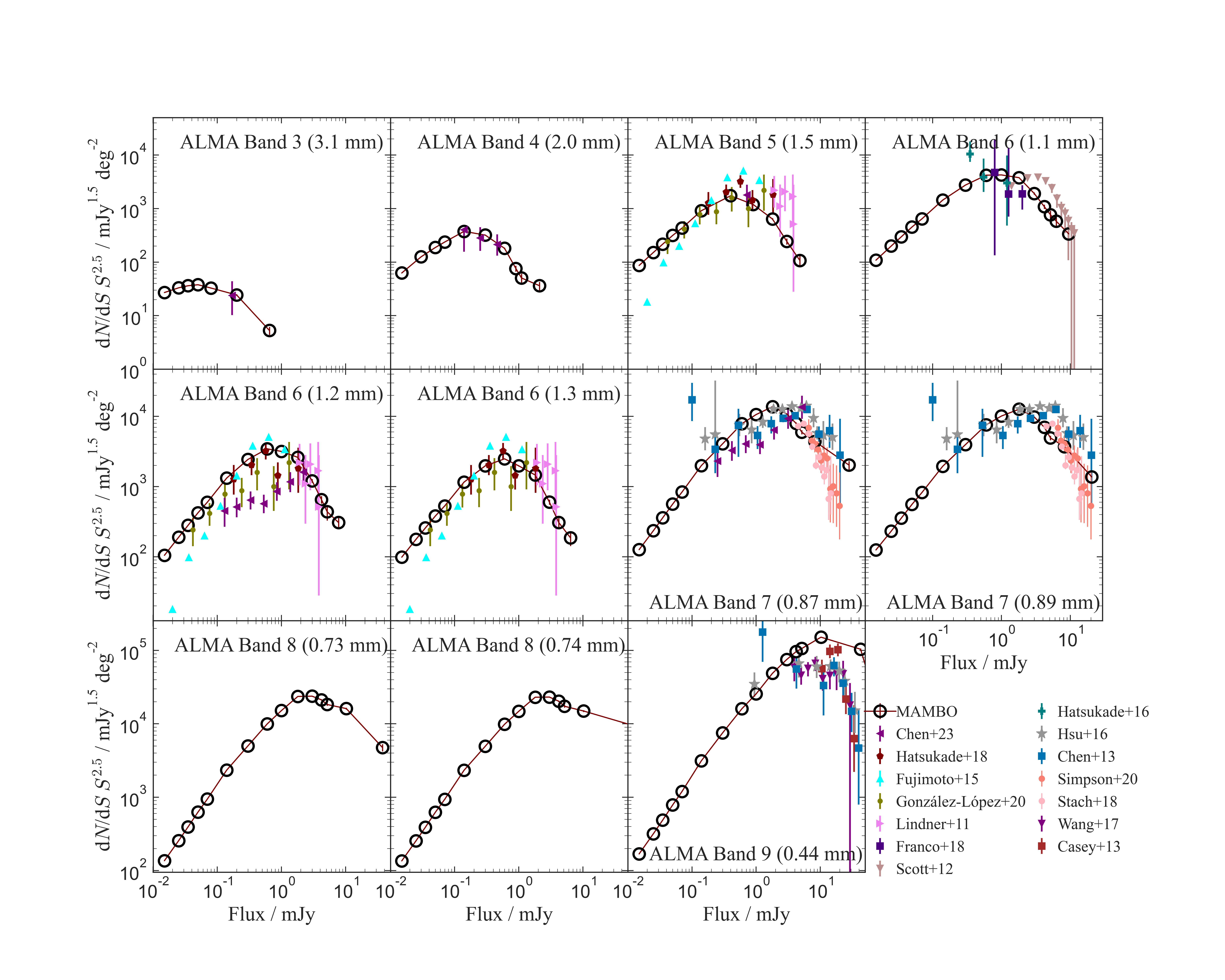
In this section, we examine the mock’s ability to reproduce observed FIR number counts. We calculate the surface density of sources per flux density interval, ${\rm d}N/{\rm d}S$, for all galaxies in the mock. These counts are a simple measure of a population’s abundance and an important tool for model comparison. Figures 3–7 show the Euclidianised differential counts (${\rm d}N/{\rm d}S\,S^{2.5}$) for the MAMBO mock at various FIR wavelengths, compared with the published estimates. The cumulative counts are presented in Appendix B.

In Fig. 3, the Spitzer-MIPS number counts from MAMBO at $24\,$\mathrm{\SIUnitSymbolMicro m}$$ and $160\,$\mathrm{\SIUnitSymbolMicro m}$$ are generally well matched to the literature, with the exception of the Lagache et al. (2004) model in the $160\,$\mathrm{\SIUnitSymbolMicro m}$$ differential counts, whose predicted peak deviates from the plotted data. There is tension between MAMBO and the data for Spitzer-MIPS (Fig. 3) and Herschel-PACS (Fig. 4) at $70\,$\mathrm{\SIUnitSymbolMicro m}$$. For both these $70\,$\mathrm{\SIUnitSymbolMicro m}$$ bands, we see an overestimation in the MAMBO counts at fluxes greater than approximately $10\,$mJy. We calculate a maximum discrepancy at the bright-flux end of the differential counts of $5\sigma$ and $6\sigma$ for MIPS and PACS, respectively. We define $\sigma$ based on the uncertainty of the published counts that show the largest discrepancy from the MAMBO counts. This discrepancy at $70\,$\mathrm{\SIUnitSymbolMicro m}$$ could partly be a result of the dust temperature used in the MAMBO mock. The $70\,$\mathrm{\SIUnitSymbolMicro m}$$ emission, at all redshifts, is on the Wien tail of an SED for the majority of dust temperatures. This means that the $70\,$\mathrm{\SIUnitSymbolMicro m}$$ emission is susceptible to contributions from hot dust. The mock could include hot dust which may result in an overestimation of the number counts at the bright, and generally low-$z$ end of $70\,$\mathrm{\SIUnitSymbolMicro m}$$, but has less effect on the FIR wavelengths. While AGN typically dominate mid-IR emission at shorter wavelengths (e.g., the $24\,$\mathrm{\SIUnitSymbolMicro m}$$ band), their contribution at $70\,$\mathrm{\SIUnitSymbolMicro m}$$ is generally modest. Therefore, neglecting AGN emission is unlikely to significantly affect the number counts at $70\,$\mathrm{\SIUnitSymbolMicro m}$$, especially at the bright end, where star formation dominates the dust heating. In addition to the discrepancy at MIPS $70\,$\mathrm{\SIUnitSymbolMicro m}$$, the bright-flux end of the MAMBO $100\,$\mathrm{\SIUnitSymbolMicro m}$$ (Fig. 4) differential counts are in excess of the published estimates (by about $2$–$3\,\sigma$) at fluxes greater than $40\,$mJy. The Lagache et al. (2004) model here is also in disagreement with the differential counts peak of the other data.

Figure 3: Differential number counts of the MAMBO mock for the Spitzer-MIPS bands. Data and models from the following works are shown for comparison: Lagache et al. (2004), Dole et al. (2004), Papovich et al. (2004), Frayer et al. (2006), Frayer et al. (2009), Shupe et al. (2008), Berta et al. (2010), Clements et al. (2011), Béthermin et al. (2010a), and Magnelli et al. (2013).

Figure 4: Differential number counts of the MAMBO mock for the Herschel-PACS bands. The legend in the $100\,$\mathrm{\SIUnitSymbolMicro m}$$ panel also applies to the $160\,$\mathrm{\SIUnitSymbolMicro m}$$ panel, and vice versa. Data and models from the following works are shown for comparison: Lagache et al. (2004), Frayer et al. (2006), Berta et al. (2010), Clements et al. (2011), Béthermin et al. (2010b), and Magnelli et al. (2013).

Figure 5: Differential number counts of the MAMBO mock for the Herschel-SPIRE bands. The legend in the $250\,$\mathrm{\SIUnitSymbolMicro m}$$ and $350\,$\mathrm{\SIUnitSymbolMicro m}$$ panels apply to all three panels. Data and models from the following works are shown for comparison: Lagache et al. (2004), Frayer et al. (2006), Berta et al. (2010), Clements et al. (2011), Béthermin et al. (2010b), and Magnelli et al. (2013).

Figure 6: Differential number counts of the MAMBO mock for the SCUBA-2 bands, Apex-LABOCA $870\,$\mathrm{\SIUnitSymbolMicro m}$$ band, and AzTec $1.1\,$mm band. Data and models from the following works are shown for comparison: Wang et al. (2017), Casey et al. (2013), Geach et al. (2013), Gao et al. (2024), Zavala et al. (2017), Lagache et al. (2004), Coppin et al. (2006), Knudsen et al. (2008), Zemcov et al. (2010), Borys et al. (2003), Béthermin et al. (2020), Karim et al. (2013), Simpson et al. (2015), Chen et al. (2023), Hsu et al. (2016), Simpson et al. (2020), and Stach et al. (2018).

Figure 7: Differential number counts of the MAMBO mock for various ALMA bands. Data and models from the various works are shown for comparison.

For the Herschel-SPIRE counts (Fig. 5), the $250\,$\mathrm{\SIUnitSymbolMicro m}$$ counts are generally in agreement with the data. However, in the differential counts at $350\,$\mathrm{\SIUnitSymbolMicro m}$$ and $500\,$\mathrm{\SIUnitSymbolMicro m}$$, we see MAMBO underestimating the number counts compared to the existing data, at flux densities between approximately $10$ and $50$ mJy. At $350\,$\mathrm{\SIUnitSymbolMicro m}$$, the Pearson et al. (2019) model also underestimates the observed differential counts and at $500\,$\mathrm{\SIUnitSymbolMicro m}$$, both the Pearson et al. (2019) and Lagache et al. (2004) models underestimate the observed differential counts. This disagreement between models and observation is explored in Béthermin et al. (2017). Their own simulation also underestimates the Herschel-SPIRE counts at similar fluxes to MAMBO ($5$–$50$ mJy). In limited angular resolution instruments such as Herschel-SPIRE, one reason for this could be the blending of several sources within the SPIRE beam. Béthermin et al. (2017) highlight the importance of taking into account resolution and clustering effects before comparing simulated catalogues with observations. They also find that their number counts (at $5$–$50$ mJy) extracted from simulated maps are in better agreement with the observed data. Creating and analysing simulated maps from the MAMBO lightcone is not something explored in this work, but would be a path for future work.

A discrepancy is also observed for SCUBA-2 at $450\,$\mathrm{\SIUnitSymbolMicro m}$$ (Fig. 6) where the mock overpredicts the differential number counts at about $7\,$mJy, with the largest discrepancy being about $4\sigma$. The only difference between the MAMBO data for the two SCUBA-2 wavelengths is the type of transmission curve used in the simulation. For $850\,$\mathrm{\SIUnitSymbolMicro m}$$ the transmission curve measured during the instrument’s performance was used and so it includes the effects of atmospheric absorption. For $450\,$\mathrm{\SIUnitSymbolMicro m}$$, the model transmission curve was used and thus did not include the effects of atmospheric absorption. A $450\,$\mathrm{\SIUnitSymbolMicro m}$$ transmission curve including the effects of atmospheric effects was not available. Since the atmosphere is significantly more opaque at $450\,$\mathrm{\SIUnitSymbolMicro m}$$, the use of the model transmission curve likely results in an overestimate of the effective throughput and, consequently, the observed fluxes in the mock catalogue. This may help explain the overprediction in number counts at $450\,$\mathrm{\SIUnitSymbolMicro m}$$ around $7\,$mJy, a discrepancy that is not as apparent at $850\,$\mathrm{\SIUnitSymbolMicro m}$$, where realistic transmission losses were properly included. The SCUBA-2 $850\,$\mathrm{\SIUnitSymbolMicro m}$$ MAMBO counts show an overall good agreement with the literature. The MAMBO $870\,$\mathrm{\SIUnitSymbolMicro m}$$ number counts (Fig. 6) are generally in good agreement with the published data at the bright-flux end, but MAMBO seems to overpredict the counts at intermediate fluxes, with a maximum discrepancy of about $6\sigma$. However, this discrepancy arises from comparing the mock counts with only one available dataset. A similar overprediction is seen for the AzTEC $1.1\,$mm counts (Fig. 6) where MAMBO portrays an excess at about $1\,$mJy, with a maximum discrepancy of $3\sigma$ from the differential counts.

The ALMA counts (Fig. 7) show an overall good agreement with results from the literature, although some discrepancies are evident at the bright-flux end for ALMA Band $7$. Since no Band $7$ number counts were available for direct comparison, we adopt the $850\,$\mathrm{\SIUnitSymbolMicro m}$$ counts as a proxy, given the similar central wavelengths. While the mock and observed counts are broadly consistent at fainter fluxes, the MAMBO mock predicts a higher number density of bright sources. This discrepancy may in part reflect the idealised nature of the mock which assumes perfect source extraction and no confusion or blending; these effects may bias observational counts at the bright end. Additionally, minor differences in the effective wavelengths ($870/890\,$\mathrm{\SIUnitSymbolMicro m}$$ versus $850\,$\mathrm{\SIUnitSymbolMicro m}$$) may introduce SED-dependent flux offsets that further contribute to the apparent excess in the MAMBO counts. In Fig. 7, for ALMA Band $9$ counts, MAMBO predicts a higher abundance of sources at the peak and bright-flux end of the differential counts than the published results. We see a maximum discrepancy of $7\sigma$ at this bright-flux end.

There are some wavelengths at which the bright-end tail of the literature counts extend past the bright-end tail of the MAMBO number counts. This is seen at the SPIRE wavelengths as well as MIPS $24\,$\mathrm{\SIUnitSymbolMicro m}$$ and PACS $70\,$\mathrm{\SIUnitSymbolMicro m}$$. The truncation in the MAMBO counts is due to the relatively small area of the MAMBO lightcone.

Overall, the MAMBO mock is generally able to reproduce the observed abundance of galaxies at the various wavelengths for both integral and differential counts.

3.3 IRLF

3.3.1 The total IR luminosity function

We derive the total IRLF for all galaxies in the MAMBO lightcone, applying an $L_{\mathrm{IR}}$ cut of $\operatorname{log_{10}}(L_{\mathrm{IR}}/L_{\odot})>8$. This luminosity threshold ensures inclusion of sources that are luminous in the FIR. Our LFs are calculated using the $1/V_{\mathrm{max}}$ method (Schmidt 1968). The MAMBO sample is sorted into redshift bins over the redshift range of the lightcone, $z\in[0.02,10]$, as in Gruppioni et al. (2013) and Rodighiero et al. (2010). The sources are sorted into $L_{\mathrm{IR}}$ bins, over the range $8\leq\operatorname{log_{10}}(L_{\mathrm{IR}}/L_{\odot})\leq 14$, each with a width of $0.5$ dex. In each $L_{\mathrm{IR}}$ bin we compute the comoving volume available to each source within that bin, defined as $V_{\mathrm{max}}=V_{z_{\mathrm{max}}}-V_{z_{\mathrm{min}}}$. Since we include all galaxies within the mock for this case, we define $V_{z_{\mathrm{max}}}$ and $V_{z_{\mathrm{min}}}$ as the upper and lower boundaries, respectively, of the redshift bin under consideration. The IRLF is then calculated using

$$\phi(L,z)=\frac{1}{\Delta\operatorname{log_{10}}(L_{\rm{IR}}/L_{\odot})}\sum_{i}\frac{1}{V_{\mathrm{max},i}},$$ (1)

where $\Delta\operatorname{log_{10}}(L_{\rm{IR}}/L_{\odot})$ is the width of the logarithmic luminosity bin and $V_{\mathrm{max},i}$ is the comoving volume over which the $i$th galaxy can be observed.

Figure 8: Total IRLF of all the galaxies within the Euclid MAMBO mock, shown as the red circles. Various data that best match the defined redshift bins are plotted for comparison. Papers referenced in short-form in the plot are defined as follows: G13: Gruppioni et al. (2013), M16: Marchetti et al. (2016), R10: Rodighiero et al. (2010), V10: Vaccari et al. (2010), F05: Le Floc’h et al. (2005), M11: Magnelli et al. (2011), F24: Fujimoto et al. (2024), G20: Gruppioni et al. (2020), B23: Barrufet et al. (2023), W19: Wang et al. (2019), and H18: Hatsukade et al. (2018).

We show the total IRLF in Fig. 8. The MAMBO mock is denoted by the red circles and relevant literature results are over-plotted. We find excellent overall agreement with the literature. At $z>6$, the scarcity of observational data renders comparison more difficult. Some notable cases of discrepancy are discussed below. At $z=1.0$–$2.0$ and $z=3.0$–$4.0$, the faint end of the Fujimoto et al. (2024) IRLF has a steeper slope than the MAMBO IRLF, with a difference of $2\sigma$. Note that it is the only published data to extend to such faint luminosities. In the $z=6.0$–$7.5$ redshift bin, the MAMBO IRLF exhibits a slightly higher normalisation than the Barrufet et al. (2023) results, with a maximum discrepancy of $4\sigma$. The Barrufet et al. (2023) data are based on a UV-selected sample, which implies that their sample does not account for extremely dust-obscured sources that are UV-faint, leading to the lower normalisation of the Barrufet et al. (2023) LF compared to the MAMBO IRLF. The Fujimoto et al. (2024) result for this redshift bin is also inconsistent with the MAMBO IRLF ($2\sigma$ discrepancy). Fujimoto et al. (2024) consistently predict a higher density of sources at the faint end of the luminosity function compared with MAMBO. The faint-end slope of the IRLF is difficult to constrain, as reflected in the sparsity of data at higher redshifts. However, in their analysis, Fujimoto et al. (2024) note that while their faint-end probes $1$–$2\,$ dex deeper than other published results, their results overall agree within $1\sigma$. Most of these comparison data cover luminosity ranges that focus on $L^{*}$, while Fujimoto et al. (2024) probe to fainter luminosities ($\sim 10^{10}L_{\odot}$) beyond the knee of the IRLF. Their faint-end results are consistent with MAMBO within $2\sigma$ uncertainties. Additionally, their sample consists of sources with ALMA data, providing greater sensitivity and higher resolution which can allow exploration below the single-dish confusion limit and reduce the impact of the incompleteness of identifying faint sources. We also cannot rule out the possibility that, since their results consistently predict a steeper slope at the faint end than MAMBO and the available data, MAMBO may be underestimating the density of fainter sources. Overall, however, the MAMBO mock reproduces the majority of observational IRLFs and, in some cases, probes to fainter luminosities than the existing data.

3.3.2 IRLF; EWS versus EDS

To explore the differences between the EWS and EDS, we compare the IRLF of all galaxies in the sample after applying AB magnitude cuts corresponding to the $5\sigma$ point-source detection limits for each Euclid band ($Y_{\scriptscriptstyle\rm E}$, $J_{\scriptscriptstyle\rm E}$, $H_{\scriptscriptstyle\rm E}$, and $I_{\scriptscriptstyle\rm E}$) in the EWS and EDS, respectively, as listed in Table 1. For this comparison, we extract sources detectable in each band given the respective survey’s magnitude limits and apply the same $L_{\mathrm{IR}}$ cut as before. The comoving volume $V_{\mathrm{max}}$ is computed for each source. In this case, $z_{\mathrm{min}}$ corresponds to the lower boundary of the redshift bin, while $z_{\mathrm{max}}$ is defined as the lesser of the upper redshift boundary and the redshift at which the source falls below the survey’s detection limit in the relevant Euclid band. The resulting IRLF is then calculated using Eq. (1) and shown in Fig. 9. For a clearer comparison, we only plot the $I_{\scriptscriptstyle\rm E}$ band for the majority of our redshift bins. The total IRLF (red circles) represents the full IRLF and any deviations from this are attributed to incompleteness introduced by the Euclid magnitude cuts. In other words, there are some IR galaxies that are undetectable by Euclid at any redshift.

We calculate the ratio of Euclid-detectable IR sources to the total population of IR sources for each $(L,z)$ bin. These results are shown in Figs. 10 and 11 for the EWS and EDS, respectively. In the first two redshift bins of Fig. 10, the fraction of IR-detectable galaxies in the $I_{\scriptscriptstyle\rm E}$ Wide sample is greater than $80\%$ at approximately $\operatorname{log_{10}}(L_{\rm{IR}}/L_{\odot})>10$, after which the percentage falls below $80\%$ in the remaining redshift bins. In the first three redshift bins of Fig. 11, $100\%$ of all IR galaxies are detectable by the EDS at $\operatorname{log_{10}}(L_{\rm{IR}}/L_{\odot})>9.5$ leading to the overlap between the EDS and total IRLF in Fig. 9 at these luminosities. Beyond $z=4$, the fraction of the EDS-detectable sample falls with redshift. The downturn in the $I_{\scriptscriptstyle\rm E}$ band for the EWS at high $L_{\rm IR}$ in the $2.5<z<4$ and $4<z<5$ bins likely reflects the increasing fraction of heavily dust-obscured, optically redder and UV-fainter systems at the highest infrared luminosities such that a larger fraction falls below the EWS $I_{\scriptscriptstyle\rm E}$ detection threshold. This effect is much less pronounced in the EDS fields, whose greater depth recovers a larger fraction of these optically faint, high-$L_{\rm IR}$ galaxies, supporting an interpretation driven primarily by depth-limited detectability rather than intrinsic changes in the IR population.

At $z=7.5$, no optical light is detected in the $I_{\scriptscriptstyle\rm E}$ band, and thus no IRLF is shown in Fig. 9 for this band. For the highest two redshift bins, we instead compare the IRLF of the $J_{\scriptscriptstyle\rm E}$ band for the EWS and EDS. Although MAMBO predicts that galaxies will be visible at these redshifts, the EDS $J_{\scriptscriptstyle\rm E}$ sample only detects $80\%$ or more of the total sample at approximately $\operatorname{log_{10}}(L_{\rm{IR}}/L_{\odot})>11$, whereas, for the same redshifts the EWS $J_{\scriptscriptstyle\rm E}$ band mostly recovers less than $30\%$ of the total IR sample. Finally, we test whether the choice of luminosity bin size affects the shape of the IRLF by recalculating it with smaller and larger bin widths. No significant changes in the overall IRLF shape are found across the tested binning schemes.

Table 1: $5\sigma$ point-like source magnitude limit of each Euclid band in the EWS and EDS, from Euclid Collaboration: Scaramella et al. (2022) and Euclid Collaboration: Selwood et al. (2025), respectively.

Band	$\lambda_{\mathrm{eff}}$ [Å]	EWS limiting mag	EDS limiting mag
$I_{\scriptscriptstyle\rm E}$	$7200$	$26.2$	$28.2$
$Y_{\scriptscriptstyle\rm E}$	$10\,810$	$24.3$	$26.3$
$J_{\scriptscriptstyle\rm E}$	$13\,670$	$24.5$	$26.5$
$H_{\scriptscriptstyle\rm E}$	$17\,710$	$24.4$	$26.4$

Figure 9: $1/V_{\rm max}$-derived IRLF for the EDS-detectable sample compared to the EWS-detectable sample. Additionally plotted for comparison is the total IRLF of all the galaxies within the Euclid MAMBO mock, shown by the red circles.

Figure 10: Fraction of detectable IR sources in the different Euclid bands in various $z$ bins for the EWS.

Figure 11: Fraction of detectable IR sources in the different Euclid bands in various $z$ bins for the EDS.

3.3.3 IRLF in different environments

We also examine how the IRLF depends on environment. To do this, we sort galaxies into three categories based on their environment; i.e., whether they are located within a cluster, protocluster, or field, based on the definitions outlined below.

We first apply a lower redshift cut of $z=1.5$ to the MAMBO mock. This threshold ensures that the redshift range includes many protoclusters, since large-scale structures are not yet fully assembled at these epochs. Galaxies are further selected using the magnitude criteria $H_{\scriptscriptstyle\rm E}\leq 24.25$ or $I_{\scriptscriptstyle\rm E}\leq 25.10$, corresponding to the expected $5\sigma$ detection limits of the EWS for extended sources.

Protocluster members are defined as galaxies associated with the same collapsed cluster by $z=0$, where the final halo mass must satisfy $M\geq 10^{14}\,M_{\odot}$. This lower mass threshold provides an operative definition for identifying massive protoclusters. In contrast, cluster members are defined as galaxies that reside within the same halo at the redshift they are observed, where the halo mass must be $M\geq 10^{13.25}\,M_{\odot}$. This threshold aligns with the mass limit used in the Euclid Cluster Finder Challenge (Adam et al. 2019). Cluster member galaxies are available only in the redshift range $1.5\leq z\leq 4.0$ because of the original constraints of the GAEA lightcone (Hirschmann et al. 2016); therefore, no cluster galaxies are included at $z>4$ for consistency between lightcones. There is an overlap between galaxies classified as cluster and protocluster members. This is expected, since a galaxy may reside in a cluster at a given redshift while also being part of a larger halo system that will evolve into a massive cluster by $z=0$. Consequently, the environment-dependent luminosity functions derived here are not mutually exclusive.

Field galaxies are defined to inhabit regions of average or low density. That being said, there could be cases of galaxies found outside clusters (i.e., in the field) that are located in regions with densities larger than the average. At the same time, galaxies on the outskirts of protoclusters, and hence characterised as protocluster member galaxies, are likely to be in average density environments. Therefore, if all cluster and protocluster member galaxies were removed from the original MAMBO mock, the remaining galaxies: (1) might include some located in high-density regions; and (2) might not constitute a complete sample, since some galaxies would have been excluded by the protocluster definition. While this approach introduces these potential limitations, it provides a practical definition suitable for comparative analysis and so we choose to define field galaxies as those that remain after the cluster and protocluster members are removed.

In Fig. 12, we present the completeness-corrected IRLF of EWS-detectable MAMBO galaxies classified by environment for a range of redshift intervals. Since the comoving volume occupied by each environment per redshift bin is not accounted for, we do not compare the normalisation of the IRLFs directly. Instead, we compare their shapes and how they evolve with redshift. To facilitate this comparison, we normalise each IRLF such that $\operatorname{log_{10}}(\phi/\rm{Mpc^{-3}\rm{dex^{-1}}})=1$ at $\operatorname{log_{10}}(L_{\mathrm{IR}}/L_{\odot})=11.5$ within each redshift bin.

Figure 12: Completeness-corrected IRLF of MAMBO mock galaxies based on their environment: cluster, protocluster, or field. The LFs are normalised such that $\operatorname{log_{10}}(\phi/\rm{Mpc}^{-3}dex^{-1})=1$ at $\operatorname{log_{10}}(L_{\mathrm{IR}}/L_{\odot})=11.5$ for each redshift bin. The legend for protocluster member galaxies also applies to field member galaxies.

We restrict our Schechter function fits to the IRLFs in Fig. 12 to the range $10.5\leq\operatorname{log_{10}}(L_{\mathrm{IR}}/L_{\odot})\leq 13.5$, since this is where the EDS and EWS IRLFs are more complete. This choice ensures that the fits are less biased by incompleteness and flux limits, which can artificially flatten or steepen $\alpha$ when low-luminosity bins are not robustly constrained. Although this excludes the classical faint end of the IRLF, it yields a more robust fit to the well-sampled portion of the data. The resulting $\alpha$ values should therefore be interpreted as effective slopes across this brighter luminosity range rather than as true faint-end slopes. As such, the absolute values of $\alpha$ are less robust than the relative trends with redshift and environment. Our results are shown in Fig. 13.

Figure 13: Redshift evolution of the completeness-corrected faint-end slope parameter $\alpha$ for different environments.

For cluster and protocluster environments, we observe a flattening of the $\alpha$ parameter with increasing redshift. For field galaxies, the $\alpha$ parameter remains approximately constant with redshift. The observational analysis of (super)cluster IRLFs is limited to low redshifts ($z<1$), which makes it difficult to compare with the MAMBO predictions which probe $z\geq 1.5$. For field galaxies, there is a greater amount of published data available. There is broad consensus that the luminosity of IR galaxies increases while their number density decreases with redshift (Caputi et al. 2007; Magnelli et al. 2011; Gruppioni et al. 2013, 2020; Traina et al. 2024), however, we cannot compare the evolution of $L^{*}$ and $\phi^{*}$ from our Schechter function fits with Fig. 12 since the functions are not scaled to the comoving volume of each environment.

Bai et al. (2009), who studied the IRLF of local clusters ($z\leq 0.06$), fixed the faint-end slope parameter to $\alpha=1.41$ in their Schechter function fits for galaxies with $\log_{10}(L_{\mathrm{IR}}/L_{\odot})\gtrsim 9$. Bai et al. (2006) examined the IRLF of the Coma cluster ($z<0.1$) and also explored its dependence on local density. They found a shallower faint-end slope ($\alpha\sim 1.0$), again fitting for $\log_{10}(L_{\mathrm{IR}}/L_{\odot})\gtrsim 9$, and observed a deficit of IR-luminous galaxies in the dense cluster core relative to lower-density outskirts. At $z=0.23$, Biviano et al. (2011) fitted a single power law to the IRLF of the A1763 cluster and found a faint-end slope of $\alpha\sim-2.0$, applying a lower luminosity cut of $\log_{10}(L_{\mathrm{IR}}/L_{\odot})\sim 10.4$. We note that in this power-law parameterisation, $\alpha$ is negative by convention, with steeper slopes (larger absolute values) indicating a more rapid increase in number density toward lower luminosities, which is physically expected for most luminosity functions. This increase in number density is also evident, for the same luminosity range as in Biviano et al. (2011), in Fig. 12 across most redshift bins.

To further assess the observational reach of the EWS, we apply an additional detection constraint that requires galaxies to be observed both by Euclid and by a NIR/FIR instrument, specifically, Herschel-PACS (Poglitsch & Altieri 2009) and Herschel-SPIRE (Griffin et al. 2010). A SPIRE detection is defined as a greater than $3\sigma$ detection in each band, with flux density thresholds based on confusion noise: $17.4\,$mJy at $250\text{\,}\mathrm{\SIUnitSymbolMicro m}$, $18.9\,$mJy at $350\text{\,}\mathrm{\SIUnitSymbolMicro m}$, and $20.4\,$mJy at $500\text{\,}\mathrm{\SIUnitSymbolMicro m}$ (Nguyen et al. 2010). For PACS, we adopt the $3\sigma$ flux density limits from the Herschel GOODS-S survey, with Herschel GOODS-S probing a little deeper than Herschel GOODS-N: $0.8\,$mJy at $100\text{\,}\mathrm{\SIUnitSymbolMicro m}$ and $2.4\,$mJy at $160\text{\,}\mathrm{\SIUnitSymbolMicro m}$ (Elbaz et al. 2011).

Prior to applying these limits to the environment-dependent IRLFs, we compute the IRLF for all MAMBO galaxies potentially detected by both EWS and PACS/SPIRE. We first filter the lightcone with the EWS detection limits and then further select only those sources that meet the PACS/SPIRE thresholds. The IRLFs are then recalculated using these filtered samples. In Fig. 14, we show the completeness-corrected IRLF for the EWS$+$SPIRE-detectable sample and the EWS$+$PACS-detectable sample. The IRLFs for the EWS$+$PACS-detectable galaxies display greater variation than those that are EWS$+$SPIRE-detectable due to Poisson statistics, because of the increased depth of the Herschel GOODS-S survey and the correspondingly larger galaxy sample. As such, we see that the small number of galaxies being selected based on the SPIRE flux limits hinders the effectiveness of this IRLF. Galaxies are present only over a small luminosity range, yielding limited interpretive value. With the deeper limits of the PACS survey, a greater sample of galaxies remain after the selection limits are applied. This results in a clear redshift evolution of the IRLF for the EWS$+$PACS-detectable sample.

Figure 14: Completeness-corrected IRLF of all MAMBO galaxies that are potentially detected by the EWS and SPIRE/PACS. Very few galaxies remain after the EWS$+$SPIRE limits are applied, so we do not see much evolution in the IRLF. For the EWS$+$PACS limits, more galaxies are detectable and we see a redshift evolution of the IRLF.

With the addition of the SPIRE and PACS limits, we then calculate the completeness-corrected IRLF for the environmental-dependent sample and show our results in Fig. 15. In the top row, the EWS$+$PACS limits are applied. Here, the IRLF for cluster and protocluster members has been normalised at $\operatorname{log_{10}}(L_{\mathrm{IR}}/L_{\odot})=13.125$ and the field IRLFs at $\operatorname{log_{10}}(L_{\mathrm{IR}}/L_{\odot})=12.25$. In the bottom row, the EWS$+$SPIRE limits are applied. Here, the IRLF for cluster and protocluster members are also normalised at $\operatorname{log_{10}}(L_{\mathrm{IR}}/L_{\odot})=13.125$ and the field IRLFs at $\operatorname{log_{10}}(L_{\mathrm{IR}}/L_{\odot})=12.5$. In both the top and bottom rows, any luminosity bin with only one source is shown as a $3\sigma$ upper limit denoted by a downward arrow.

Cluster member galaxies are present only until $z=4$ and it is in this high-redshift bin ($z=3.5$–$4$) where the EWS$+$SPIRE is able to detect them, but only over a small range at the highest luminosities; $12.6\leq\log(L_{\mathrm{IR}}/L_{\odot})\leq 13.6$. At lower redshifts, cluster member galaxies are predicted to be undetectable simultaneously by the EWS and SPIRE. Similarly, protocluster members are detectable only in the $z=3.5$–$4$ redshift bin. The shape of the IRLF for field galaxies at different redshifts remains unchanged over the small luminosity range shown. It should be noted that, due to the small area of the MAMBO lightcone (approximately $3\text{\,}\deg\mathrm{{}^{2}}$), only a small number of galaxies remain after the EWS$+$SPIRE detection limits are applied, leading to the large Poisson errors seen in Fig. 15. The EWS$+$PACS limits (top row of Fig. 15) give similar results for cluster and protocluster members as the bottom row with EWS$+$SPIRE limits. The only galaxies visible are those in the $z=3.5$–$4$ redshift bin. The IRLF for EWS$+$PACS-detectable field galaxies is comparable to the IRLF in Fig. 12. We see a clear decreasing trend for all redshifts in the IRLF for luminosities larger than $10^{11.75}\,L_{\odot}$, with little redshift variation in the shape of the function.

However, given that the PACS observations of the Herschel GOODS-S field cover $100\,$arcmin² in about $200$ hours, and PACS observations of a similar area and depth to MAMBO do not exist, these results are only a modest theoretical insight into the IRLF for field galaxies, and the reality of achieving this is unlikely without a new FIR mission.

Figure 15: Top row: Completeness-corrected IRLF of MAMBO mock galaxies based on their environment given that they are detected by the EWS and Spitzer-PACS. The cluster and protocluster LFs are normalised at $\operatorname{log_{10}}(L_{\mathrm{IR}}/L_{\odot})=13.125$ and the field LFs at $12.25$. $3\sigma$ upper limits, denoted by a downwards arrow, are shown where there is only one source per luminosity bin. The legend in the top row also applies to the bottom row. Bottom row: Completeness-corrected IRLF of MAMBO mock galaxies based on their environment, given that they are detected by the EWS and Herschel-SPIRE. The cluster and protocluster apparent LFs are normalised at $\operatorname{log_{10}}(L_{\mathrm{IR}}/L_{\odot})=13.125$ and the field LFs at $12.5$.

The environment dependence seen in Fig. 12 for the high-luminosity end ($L_{\mathrm{IR}}>10^{12}\,L_{\odot}$) suggests that this is a relation worth studying further, but it is clear that this will require a much larger survey area, for both simulation and observational data. Given our results for Fig. 15, specifically for the EWS$+$SPIRE-detectable sample, we estimate that a mock with an area at least $30$ times greater than the current MAMBO mock is required to achieve IRLF results that are statistically reliable (i.e., greater than $3\sigma$). Existing large-scale Herschel surveys such as HerMES (Oliver et al. 2012) and H-ATLAS (Valiante et al. 2016; Bourne et al. 2016) have much larger survey areas ($380\text{\,}\deg\mathrm{{}^{2}}$ and $600\text{\,}\deg\mathrm{{}^{2}}$, respectively) than the MAMBO lightcone. Performing a similar analysis with these surveys will provide a substantial number of FIR- and Euclid-detectable sources for a statistically useful study on the environmental dependency of the IRLF using existing data, albeit we are limited by the instruments’ sensitivity. With Herschel no longer in operation, attention must shift to other existing facilities – such as ALMA and NOEMA – which observe in the millimetre regime and can conduct wide surveys that sample the same dust-emission SEDs, albeit at longer wavelengths. Furthermore, future instruments such as the Cerro Chajnantor Atacama Telescope (CCAT; CCAT-Prime Collaboration et al. 2022), operating between $0.3$–$3\,\mathrm{mm}$, will be capable of covering large survey areas with high sensitivity, enabling improved constraints on the Rayleigh–Jeans tail and peak of the FIR SED. The PRobe far-Infrared Mission for Astrophysics (PRIMA; Moullet et al. 2023) is a future telescope concept, which, if selected, will provide additional large-area surveys at wavelengths that overlap with Herschel but probe to deeper sensitivities.

4 Conclusions

With the FIR extension of the MAMBO lightcone, we investigated the predicted FIR properties of Euclid-detectable galaxies and validated MAMBO’s capacity to reproduce observed number counts and IRLFs. Furthermore, in preparation for upcoming Euclid observations, we investigated its capability to detect NIR/FIR-detectable sources and assess the dependence of IRLFs on the galaxy environment. The main results of this study are summarised as follows.

1. The predicted FIR flux densities of star-forming galaxies follows the expected trends with increasing redshift and highlights that only the brightest FIR galaxies will be detectable by Euclid. Their predicted dust temperatures and IR luminosities generally increase with redshift, as expected, and their dust masses remain relatively constant with redshift.

2. The MAMBO lightcone reproduces FIR number counts well across most bands. In some cases, the predicted number counts extend to fainter fluxes than the existing counts, offering model predictions at the faint end to compare with future data.

3. The total IRLF calculated for the entire MAMBO sample shows excellent agreement with the published data across most redshift bins (see Fig. 8). At redshifts $z>6$, the sparsity of observational data prevents strong conclusions.

4. Comparing the IRLF for the EWS- and EDS-detectable samples (Fig. 9), we find similar IRLF shapes at $0.02<z<4$, particularly at $\operatorname{log_{10}}(L_{\mathrm{IR}}/L_{\odot})>10$ where the fraction of IR-detectable sources is the highest ($>80\%$). With increasing redshift, we see a greater deviation from the total IRLF by the EWS sample, while the greater depth of the EDS is able to select a higher fraction of IR galaxies out to $z=6$. At $z>6$, the $I_{\scriptscriptstyle\rm E}$ band is no longer effective due to the redshifted Lyman limit, although galaxies remain detectable in the NIR bands with both surveys, up to the highest redshifts albeit at much smaller fractions. Our ratio of IR-detectable sources in the Euclid surveys will enable observed Euclid IRLFs to be corrected for the missing populations entirely undetectable by Euclid.

5. By fitting the Schechter function to the environment-dependent IRLF, we observe a moderate flattening of the faint-end slope $\alpha$ with increasing redshift, for cluster and protocluster environments. The slope for field galaxies remains approximately constant with redshift.

6. By applying additional NIR/FIR detection constraints based on the flux limits of Herschel-PACS and SPIRE, we explore the IRLF’s environmental dependence (Fig. 15). Cluster and protocluster galaxies, for both sets of limits, are detectable only in the $z=3.5$–$4$ bin and only at high luminosities ($L_{\mathrm{IR}}>10^{12.5}\,L_{\odot}$). The shape of the field IRLF for the EWS$+$SPIRE-detectable is unchanged with redshift, although the small area of the MAMBO lightcone limits the statistical utility of this sample. The EWS$+$PACS-detectable sample is more statistically robust, but since PACS observations to the required depth and area do not exist, we must rely on other existing FIR and (sub-)mm facilities, as well as upcoming FIR (concept) facilities such as PRIMA and CCAT.

7. To enable a statistically robust study of the environment dependence of the IRLF for FIR- and Euclid-detectable sources, a significantly larger simulation area than $3.14\text{\,}\deg\mathrm{{}^{2}}$ is required. Using the predictions for the EWS$+$SPIRE-detectable sample in Fig. 15, we estimate that a minimum area of $90\text{\,}\deg\mathrm{{}^{2}}$ – $30$ times the current MAMBO lightcone – is necessary to derive statistically significant results.

Overall, the FIR extension of the MAMBO mock successfully reproduces the expected trends of the FIR physical properties with redshift and highlights the expected flux ranges of FIR sources that we can study with real Euclid data. The number counts and IRLFs are mostly in agreement with the various published data. Through environment-based IRLFs – particularly with the addition of NIR/FIR detection limits – we forecast the capabilities of future Euclid observations in characterising galaxy environments. These results highlight the promise of combining Euclid with current and future FIR data/facilities and emphasise the need for larger simulated and observational fields to explore the environmental evolution of IRLFs in a statistically robust manner.

Appendix A Stacked FIR flux densities

Here we show the stacked FIR flux densities of Euclid-detectable star-forming galaxies sorted into stellar mass and redshift bins to match those in the analysis of Euclid Collaboration: Hill et al. (2025). Across all stellar mass bins, the FIR flux densities in each band show a systematic decline with increasing redshift, reflecting cosmological dimming. Comparing these average FIR flux densities with the early results of Euclid Collaboration: Hill et al. (2025), our MAMBO predictions are generally in agreement.

Table 2: Average FIR flux densities of EWS-detectable galaxies in stellar mass and redshift bins as predicted by MAMBO. We find no EWS-detectable galaxies in any of the FIR bands at $z=2.9$ for a stellar mass of $\log_{10}(\mathit{M}_{*}/M_{\odot})=8.5$; this bin is therefore not shown.

$\log_{10}$	$z$	$S_{100}$	$S_{160}$	$S_{250}$	$S_{350}$	$S_{500}$	$S_{850}$
$(M_{*}/M_{\odot})$		[mJy]	[mJy]	[mJy]	[mJy]	[mJy]	[mJy]
8.5	0.3	0.15$\pm$0.003	0.4$\pm$0.005	0.27$\pm$0.003	0.15$\pm$0.002	0.063$\pm$0.0007	0.02$\pm$0.0002
8.5	0.5	0.05$\pm$0.001	0.2$\pm$0.002	0.14$\pm$0.001	0.08$\pm$0.0006	0.035$\pm$0.0003	0.01$\pm$0.00008
8.5	0.7	0.03$\pm$0.001	0.1$\pm$0.001	0.1$\pm$0.001	0.062$\pm$0.0006	0.029$\pm$0.0003	0.0073$\pm$0.00006
8.5	0.9	0.02$\pm$0.001	0.1$\pm$0.002	0.078$\pm$0.001	0.053$\pm$0.0009	0.025$\pm$0.0004	0.0066$\pm$0.0001
8.5	1.1	0.02$\pm$0.001	0.1$\pm$0.004	0.068$\pm$0.003	0.049$\pm$0.002	0.023$\pm$0.0007	0.006$\pm$0.0002
8.5	1.3	0.02$\pm$0.002	0.1$\pm$0.006	0.07$\pm$0.004	0.051$\pm$0.003	0.023$\pm$0.001	0.006$\pm$0.0003
8.5	1.5	0.02$\pm$0.007	0.1$\pm$0.02	0.064$\pm$0.01	0.048$\pm$0.009	0.021$\pm$0.003	0.0055$\pm$0.0008
8.5	1.7	0.01$\pm$0.005	0.03$\pm$0.02	0.029$\pm$0.01	0.021$\pm$0.009	0.014$\pm$0.006	0.0032$\pm$0.001
8.5	1.9	0.001$\pm$0.001	0.01$\pm$0.002	0.0074$\pm$0.002	0.0057$\pm$0.002	0.0051$\pm$0.002	0.00096$\pm$0.0003
8.5	2.1	0.001$\pm$0.001	0.01$\pm$0.005	0.0071$\pm$0.006	0.0056$\pm$0.004	0.0038$\pm$0.002	0.001$\pm$0.0005
8.5	2.3	0.0002$\pm$0.0001	0.003$\pm$0.0006	0.005$\pm$0.001	0.0052$\pm$0.001	0.0044$\pm$0.001	0.0014$\pm$0.0004
8.5	2.5	0.0003$\pm$0.002	0.002$\pm$0.002	0.0028$\pm$0.002	0.0022$\pm$0.001	0.0033$\pm$0.002	0.00036$\pm$0.0002
8.5	2.7	0.0004$\pm$0.002	0.003$\pm$0.001	0.0049$\pm$0.002	0.0046$\pm$0.001	0.0041$\pm$0.0002	0.0011$\pm$0.0003
8.9	0.3	0.44$\pm$0.01	1.1$\pm$0.02	0.77$\pm$0.01	0.43$\pm$0.005	0.18$\pm$0.002	0.052$\pm$0.0006
8.9	0.5	0.13$\pm$0.002	0.4$\pm$0.004	0.36$\pm$0.003	0.22$\pm$0.002	0.096$\pm$0.0007	0.026$\pm$0.0002
8.9	0.7	0.06$\pm$0.001	0.3$\pm$0.002	0.24$\pm$0.002	0.15$\pm$0.001	0.072$\pm$0.0004	0.018$\pm$0.0001
8.9	0.9	0.04$\pm$0.001	0.2$\pm$0.002	0.18$\pm$0.001	0.12$\pm$0.0008	0.06$\pm$0.0004	0.016$\pm$0.0001
8.9	1.1	0.03$\pm$0.001	0.1$\pm$0.002	0.14$\pm$0.001	0.11$\pm$0.0009	0.054$\pm$0.0004	0.015$\pm$0.0001
8.9	1.3	0.02$\pm$0.001	0.1$\pm$0.002	0.12$\pm$0.002	0.095$\pm$0.001	0.049$\pm$0.0005	0.014$\pm$0.0001
8.9	1.5	0.01$\pm$0.0004	0.1$\pm$0.002	0.097$\pm$0.002	0.08$\pm$0.001	0.043$\pm$0.0006	0.013$\pm$0.0002
8.9	1.7	0.01$\pm$0.001	0.1$\pm$0.004	0.09$\pm$0.003	0.071$\pm$0.002	0.043$\pm$0.001	0.013$\pm$0.0003
8.9	1.9	0.01$\pm$0.001	0.1$\pm$0.006	0.087$\pm$0.006	0.07$\pm$0.004	0.045$\pm$0.002	0.013$\pm$0.0006
8.9	2.1	0.02 $\pm$0.007	0.1$\pm$0.04	0.14$\pm$0.04	0.11$\pm$0.03	0.063$\pm$0.01	0.017$\pm$0.003
8.9	2.3	0.004$\pm$0.001	0.03$\pm$0.007	0.043$\pm$0.009	0.038$\pm$0.007	0.027$\pm$0.005	0.0081$\pm$0.001
8.9	2.5	0.004$\pm$0.002	0.03$\pm$0.01	0.031$\pm$0.01	0.026$\pm$0.008	0.017$\pm$0.004	0.0053$\pm$0.001
8.9	2.7	0.001$\pm$0.001	0.01$\pm$0.002	0.019$\pm$0.003	0.02$\pm$0.003	0.017$\pm$0.002	0.0054$\pm$0.0007
8.9	2.9	0.001$\pm$0.0001	0.01$\pm$0.0008	0.011$\pm$0.001	0.012$\pm$0.002	0.0096$\pm$0.001	0.0036$\pm$0.0006
9.3	0.3	1.16$\pm$0.04	2.8$\pm$0.05	2$\pm$0.03	1.1$\pm$0.02	0.47$\pm$0.007	0.13$\pm$0.002
9.3	0.5	0.39$\pm$0.01	1.2$\pm$0.02	1$\pm$0.01	0.6$\pm$0.006	0.27$\pm$0.002	0.071$\pm$0.0007
9.3	0.7	0.17$\pm$0.003	0.7$\pm$0.007	0.64$\pm$0.005	0.41$\pm$0.003	0.19$\pm$0.001	0.05$\pm$0.0003
9.3	0.9	0.10$\pm$0.002	0.5$\pm$0.004	0.47$\pm$0.003	0.33$\pm$0.002	0.16$\pm$0.001	0.044$\pm$0.0003
9.3	1.1	0.06$\pm$0.001	0.4$\pm$0.004	0.38$\pm$0.003	0.29$\pm$0.002	0.15$\pm$0.001	0.041$\pm$0.0003
9.3	1.3	0.04$\pm$0.001	0.3$\pm$0.003	0.31$\pm$0.003	0.25$\pm$0.002	0.13$\pm$0.0009	0.039$\pm$0.0003
9.3	1.5	0.03$\pm$0.001	0.2$\pm$0.003	0.27$\pm$0.003	0.22$\pm$0.002	0.12$\pm$0.001	0.037$\pm$0.0003
9.3	1.7	0.03$\pm$0.001	0.2$\pm$0.004	0.25$\pm$0.004	0.2$\pm$0.002	0.13$\pm$0.001	0.038$\pm$0.0004
9.3	1.9	0.02$\pm$0.001	0.2$\pm$0.005	0.25$\pm$0.006	0.21$\pm$0.004	0.13$\pm$0.002	0.041$\pm$0.0007
9.3	2.1	0.02$\pm$0.001	0.2$\pm$0.008	0.23$\pm$0.009	0.2$\pm$0.007	0.13$\pm$0.004	0.04$\pm$0.001
9.3	2.3	0.02$\pm$0.002	0.1$\pm$0.01	0.19$\pm$0.01	0.17$\pm$0.009	0.11$\pm$0.005	0.037$\pm$0.002
9.3	2.5	0.01$\pm$0.001	0.1$\pm$0.007	0.13$\pm$0.009	0.13$\pm$0.007	0.088$\pm$0.005	0.03$\pm$0.001
9.3	2.7	0.01$\pm$0.0004	0.1$\pm$0.004	0.1$\pm$0.007	0.11$\pm$0.007	0.081$\pm$0.005	0.03$\pm$0.002
9.3	2.9	0.01$\pm$0.001	0.1$\pm$0.006	0.11$\pm$0.01	0.11$\pm$0.009	0.081$\pm$0.006	0.031$\pm$0.002
9.7	0.3	2.69$\pm$0.1	6.5$\pm$0.2	4.8$\pm$0.1	2.7$\pm$0.05	1.1$\pm$0.02	0.31$\pm$0.006
9.7	0.5	1.02$\pm$0.04	3.1$\pm$0.05	2.6$\pm$0.04	1.5$\pm$0.02	0.67$\pm$0.008	0.17$\pm$0.002
9.7	0.7	0.45$\pm$0.01	1.8$\pm$0.02	1.7$\pm$0.02	1.1$\pm$0.009	0.51$\pm$0.004	0.13$\pm$0.001
9.7	0.9	0.26$\pm$0.005	1.3$\pm$0.01	1.3$\pm$0.01	0.89$\pm$0.007	0.44$\pm$0.003	0.12$\pm$0.0008
9.7	1.1	0.18$\pm$0.004	1$\pm$0.01	1$\pm$0.01	0.77$\pm$0.006	0.4$\pm$0.003	0.11$\pm$0.0008
9.7	1.3	0.12$\pm$0.003	0.8$\pm$0.01	0.88$\pm$0.009	0.7$\pm$0.006	0.37$\pm$0.003	0.11$\pm$0.0008
9.7	1.5	0.09$\pm$0.002	0.6$\pm$0.008	0.76$\pm$0.008	0.62$\pm$0.005	0.35$\pm$0.003	0.11$\pm$0.0008
9.7	1.7	0.07$\pm$0.002	0.5$\pm$0.009	0.72$\pm$0.009	0.59$\pm$0.006	0.36$\pm$0.003	0.11$\pm$0.001
Continued on next page
9.7	1.9	0.06$\pm$0.002	0.5$\pm$0.01	0.66$\pm$0.01	0.56$\pm$0.008	0.36$\pm$0.004	0.11$\pm$0.001
9.7	2.1	0.06$\pm$0.002	0.5$\pm$0.01	0.66$\pm$0.01	0.57$\pm$0.01	0.37$\pm$0.006	0.12$\pm$0.002
9.7	2.3	0.05$\pm$0.002	0.4$\pm$0.02	0.61$\pm$0.02	0.56$\pm$0.01	0.37$\pm$0.009	0.13$\pm$0.003
9.7	2.5	0.03$\pm$0.002	0.3$\pm$0.02	0.49$\pm$0.02	0.48$\pm$0.02	0.33$\pm$0.01	0.12$\pm$0.004
9.7	2.7	0.03$\pm$0.002	0.3$\pm$0.01	0.44$\pm$0.02	0.44$\pm$0.02	0.31$\pm$0.01	0.12$\pm$0.004
9.7	2.9	0.02$\pm$0.001	0.2$\pm$0.01	0.36$\pm$0.02	0.38$\pm$0.02	0.27$\pm$0.01	0.1$\pm$0.004
10.1	0.3	6.58$\pm$0.5	15$\pm$0.5	11$\pm$0.3	5.9$\pm$0.1	2.5$\pm$0.05	0.64$\pm$0.01
10.1	0.5	2.40$\pm$0.09	7.4$\pm$0.1	6.1$\pm$0.1	3.6$\pm$0.05	1.6$\pm$0.02	0.41$\pm$0.006
10.1	0.7	1.16$\pm$0.05	4.6$\pm$0.08	4.2$\pm$0.06	2.7$\pm$0.03	1.3$\pm$0.01	0.33$\pm$0.003
10.1	0.9	0.75$\pm$0.03	3.5$\pm$0.05	3.4$\pm$0.04	2.4$\pm$0.02	1.2$\pm$0.01	0.31$\pm$0.003
10.1	1.1	0.46$\pm$0.02	2.5$\pm$0.04	2.7$\pm$0.03	2.1$\pm$0.02	1.1$\pm$0.01	0.3$\pm$0.003
10.1	1.3	0.34$\pm$0.02	2$\pm$0.03	2.4$\pm$0.03	1.9$\pm$0.02	1$\pm$0.009	0.3$\pm$0.003
10.1	1.5	0.27$\pm$0.02	1.8$\pm$0.03	2.2$\pm$0.03	1.8$\pm$0.02	1$\pm$0.01	0.31$\pm$0.003
10.1	1.7	0.21$\pm$0.01	1.5$\pm$0.03	2$\pm$0.03	1.6$\pm$0.02	1$\pm$0.01	0.31$\pm$0.003
10.1	1.9	0.16$\pm$0.01	1.3$\pm$0.03	1.8$\pm$0.03	1.5$\pm$0.02	0.97$\pm$0.01	0.31$\pm$0.004
10.1	2.1	0.15$\pm$0.01	1.2$\pm$0.03	1.7$\pm$0.04	1.5$\pm$0.03	1$\pm$0.02	0.33$\pm$0.005
10.1	2.3	0.11$\pm$0.01	1$\pm$0.03	1.5$\pm$0.04	1.4$\pm$0.03	0.93$\pm$0.02	0.32$\pm$0.006
10.1	2.5	0.09$\pm$0.01	0.8$\pm$0.03	1.4$\pm$0.04	1.3$\pm$0.04	0.92$\pm$0.02	0.33$\pm$0.008
10.1	2.7	0.09$\pm$0.01	0.8$\pm$0.03	1.3$\pm$0.04	1.3$\pm$0.04	0.93$\pm$0.02	0.34$\pm$0.008
10.1	2.9	0.07$\pm$0.02	0.7$\pm$0.04	1.2$\pm$0.06	1.3$\pm$0.05	0.9$\pm$0.03	0.35$\pm$0.01
10.5	0.3	9.22$\pm$0.7	22$\pm$0.9	17$\pm$0.5	9.3$\pm$0.3	3.9$\pm$0.1	1$\pm$0.03
10.5	0.5	3.86$\pm$0.2	13$\pm$0.3	11$\pm$0.2	6.4$\pm$0.1	2.9$\pm$0.05	0.72$\pm$0.01
10.5	0.7	2.39$\pm$0.1	9.3$\pm$0.2	8.5$\pm$0.1	5.5$\pm$0.08	2.6$\pm$0.04	0.65$\pm$0.009
10.5	0.9	1.54$\pm$0.06	7.1$\pm$0.1	6.9$\pm$0.1	4.8$\pm$0.06	2.4$\pm$0.03	0.63$\pm$0.008
10.5	1.1	1.02$\pm$0.03	5.7$\pm$0.1	6$\pm$0.1	4.6$\pm$0.07	2.4$\pm$0.03	0.66$\pm$0.009
10.5	1.3	0.77$\pm$0.02	4.9$\pm$0.09	5.8$\pm$0.09	4.6$\pm$0.06	2.5$\pm$0.03	0.73$\pm$0.008
10.5	1.5	0.62$\pm$0.02	4.2$\pm$0.09	5.2$\pm$0.08	4.3$\pm$0.06	2.4$\pm$0.03	0.74$\pm$0.009
10.5	1.7	0.52$\pm$0.02	3.7$\pm$0.09	4.9$\pm$0.08	4.1$\pm$0.06	2.5$\pm$0.03	0.78$\pm$0.009
10.5	1.9	0.41$\pm$0.02	3.3$\pm$0.08	4.7$\pm$0.09	4.1$\pm$0.07	2.6$\pm$0.04	0.84$\pm$0.01
10.5	2.1	0.38$\pm$0.02	3.2$\pm$0.1	4.6$\pm$0.1	4.1$\pm$0.08	2.7$\pm$0.05	0.88$\pm$0.01
10.5	2.3	0.32$\pm$0.02	2.8$\pm$0.1	4.2$\pm$0.1	3.9$\pm$0.1	2.6$\pm$0.06	0.89$\pm$0.02
10.5	2.5	0.25$\pm$0.01	2.4$\pm$0.1	3.8$\pm$0.2	3.7$\pm$0.2	2.5$\pm$0.1	0.9$\pm$0.03
10.5	2.7	0.21$\pm$0.01	2$\pm$0.1	3.3$\pm$0.1	3.3$\pm$0.1	2.3$\pm$0.09	0.86$\pm$0.03
10.5	2.9	0.20$\pm$0.01	1.9$\pm$0.1	3.3$\pm$0.2	3.4$\pm$0.2	2.4$\pm$0.1	0.91$\pm$0.04
10.9	0.3	10.37$\pm$0.9	28$\pm$1	21$\pm$0.8	12$\pm$0.4	5.2$\pm$0.2	1.3$\pm$0.05
10.9	0.5	5.27$\pm$0.4	18$\pm$0.6	15$\pm$0.4	9.3$\pm$0.2	4.2$\pm$0.09	1.1$\pm$0.02
10.9	0.7	3.34$\pm$0.3	13$\pm$0.5	13$\pm$0.4	8.3$\pm$0.2	4$\pm$0.09	1$\pm$0.02
10.9	0.9	2.17$\pm$0.1	11$\pm$0.4	11$\pm$0.3	8.2$\pm$0.2	4.2$\pm$0.08	1.1$\pm$0.02
10.9	1.1	1.73$\pm$0.05	9.9$\pm$0.3	11$\pm$0.3	8.1$\pm$0.2	4.3$\pm$0.09	1.2$\pm$0.02
10.9	1.3	1.30$\pm$0.05	8.5$\pm$0.2	10$\pm$0.2	8.1$\pm$0.2	4.4$\pm$0.08	1.3$\pm$0.02
10.9	1.5	1.19$\pm$0.04	8.3$\pm$0.2	10$\pm$0.2	8.6$\pm$0.2	4.9$\pm$0.09	1.5$\pm$0.03
10.9	1.7	0.98$\pm$0.03	7.2$\pm$0.2	9.7$\pm$0.2	8.1$\pm$0.1	5$\pm$0.08	1.6$\pm$0.03
10.9	1.9	0.77$\pm$0.04	6.3$\pm$0.2	9.1$\pm$0.2	7.9$\pm$0.2	5.1$\pm$0.1	1.6$\pm$0.03
10.9	2.1	0.75$\pm$0.04	6.2$\pm$0.2	9.3$\pm$0.3	8.4$\pm$0.2	5.5$\pm$0.1	1.9$\pm$0.04
10.9	2.3	0.67$\pm$0.03	6$\pm$0.3	9.2$\pm$0.3	8.5$\pm$0.3	5.7$\pm$0.2	2$\pm$0.06
10.9	2.5	0.49$\pm$0.03	4.5$\pm$0.3	7.5$\pm$0.4	7.5$\pm$0.3	5.2$\pm$0.2	1.9$\pm$0.08
10.9	2.7	0.41$\pm$0.03	3.9$\pm$0.3	6.8$\pm$0.4	7.1$\pm$0.4	5.1$\pm$0.2	1.9$\pm$0.08
10.9	2.9	0.35$\pm$0.03	3.4$\pm$0.3	5.9$\pm$0.5	6.4$\pm$0.4	4.6$\pm$0.3	1.8$\pm$0.1
11.3	0.3	4.71$\pm$0.8	19$\pm$2	17$\pm$2	10$\pm$1	4.6$\pm$0.5	1.3$\pm$0.1
11.3	0.5	4.43$\pm$0.6	18$\pm$2	17$\pm$1	10$\pm$0.6	4.8$\pm$0.3	1.3$\pm$0.07
11.3	0.7	4.03$\pm$0.7	15$\pm$1	14$\pm$1	9.3$\pm$0.6	4.5$\pm$0.3	1.2$\pm$0.07
11.3	0.9	2.05$\pm$0.2	11$\pm$0.7	12$\pm$0.6	9.2$\pm$0.4	4.8$\pm$0.2	1.4$\pm$0.06
11.3	1.1	1.71$\pm$0.2	11$\pm$0.7	13$\pm$0.6	10$\pm$0.4	5.4$\pm$0.2	1.6$\pm$0.06
Continued on next page
11.3	1.3	1.89$\pm$0.2	12$\pm$0.8	14$\pm$0.7	11$\pm$0.4	6$\pm$0.2	1.8$\pm$0.06
11.3	1.5	1.56$\pm$0.1	11$\pm$0.7	14$\pm$0.6	11$\pm$0.4	6.6$\pm$0.2	2$\pm$0.06
11.3	1.7	1.29$\pm$0.1	9.9$\pm$0.5	14$\pm$0.5	12$\pm$0.4	7.2$\pm$0.2	2.3$\pm$0.07
11.3	1.9	1.39$\pm$0.1	11$\pm$0.8	15$\pm$0.8	13$\pm$0.6	8.1$\pm$0.3	2.6$\pm$0.09
11.3	2.1	1.00$\pm$0.1	8.6$\pm$0.5	13$\pm$0.6	12$\pm$0.5	8$\pm$0.3	2.8$\pm$0.1
11.3	2.3	1.39$\pm$0.2	12$\pm$1	17$\pm$2	15$\pm$1	10$\pm$0.6	3.3$\pm$0.2
11.3	2.5	1.04$\pm$0.1	9.8$\pm$1	16$\pm$2	15$\pm$2	11$\pm$1	3.8$\pm$0.3
11.3	2.7	1.07$\pm$0.3	9.9$\pm$2	16$\pm$3	15$\pm$2	10$\pm$1	3.7$\pm$0.4
11.3	2.9	0.54$\pm$0.1	5.1$\pm$0.7	9.5$\pm$1	11$\pm$1	8.1$\pm$0.7	3.3$\pm$0.3

Appendix B Integral number counts

Here, we show the integral number counts for all the bands previously mentioned in Sect. 3.2. The integral counts predicted from MAMBO are in overall agreement with the published estimates, although there are a few cases of discrepancies. Similarly to the differential counts, for MIPS and PACS at $70\,$\mathrm{\SIUnitSymbolMicro m}$$ (Fig. 16), MAMBO overestimates the integral counts at about $100\,$mJy. The MAMBO counts for rest of the MIPS and PACS bands agree well with published data. The Herschel, SCUBA-2, and LABOCA predictions from MAMBO are generally in agreement with published results. An overprediction is seen for the AzTEC $1.1\,$mm counts where MAMBO predicts an excess at about $1\,$mJy, with a maximum discrepancy of $5\sigma$ from the published estimates. In the integral counts for ALMA Band $8$ (Fig. 17), the MAMBO counts deviate by more than $10\sigma$ from the literature values (when compared to Geach et al. 2017) at fluxes $\gtrsim 5\,$mJy but we note that this is likely due to comparing Band 8 data with higher wavelength ($\sim 850\,$\mathrm{\SIUnitSymbolMicro m}$$) published data.

Figure 16: Integral counts of the MAMBO mock for various bands: MIPS, PACS, SPIRE, SCUBA-2, Apex LABOCA, and AzTEC. Data and models are shown for comparison.

Figure 17: Integral number counts of the MAMBO mock for various ALMA bands. The specific wavelength of each ALMA band is stated in each subplot. Literature counts and models are shown for comparison.