Incremental Neural Network Verification via Learned Conflicts

Abstract

Neural network verification is often used as a core component within larger analysis procedures, which generate sequences of closely related verification queries over the same network. In existing neural network verifiers, each query is typically solved independently, and information learned during previous runs is discarded, leading to repeated exploration of the same infeasible regions of the search space. In this work, we aim to expedite verification by reducing this redundancy. We propose an incremental verification technique that reuses learned conflicts across related verification queries. The technique can be added on top of any branch-and-bound-based neural network verifier. During verification, the verifier records conflicts corresponding to learned infeasible combinations of activation phases, and retains them across runs. We formalize a refinement relation between verification queries and show that conflicts learned for a query remain valid under refinement, enabling sound conflict inheritance. Inherited conflicts are handled using a SAT solver to perform consistency checks and propagation, allowing infeasible subproblems to be detected and pruned early during search. We implement the proposed technique in the Marabou verifier and evaluate it on three verification tasks: local robustness radius determination, verification with input splitting, and minimal sufficient feature set extraction. Our experiments show that incremental conflict reuse reduces verification effort and yields speedups of up to 1.9$\times$ over a non-incremental baseline.

1 Introduction

Deep neural networks (DNNs) are increasingly deployed in safety-critical applications [3], including autonomous driving [10, 30], medical diagnosis [19], and aerospace systems [18, 24]. Their strong empirical performance has driven major advances in tasks such as control and image recognition. Despite this success, neural networks remain largely opaque and difficult to reason about, raising serious concerns regarding their reliability and safety in critical settings.

To address this issue, numerous approaches have been developed for neural network verification, with the goal of providing rigorous guarantees about network behavior. For networks with piecewise-linear activation functions, such as ReLUs, the verification problem is NP-complete [24], which hinders scalability; but as neural networks are adopted across increasingly diverse and high-stakes domains, the demand for scalable verification techniques continues to grow. Improving the efficiency of neural network verification is therefore imperative.

Examining how DNN verification is used in practice, we observe that it is often not performed as a single, isolated query, but rather invoked repeatedly within larger analysis procedures. For example, in formal explainability, verification queries are issued repeatedly to reason about the contribution of different input features to a given prediction under progressively refined constraints [8, 42, 43, 12]; similarly, in robustness radius computation, verification queries are invoked iteratively to narrow down the maximum safe perturbation radius around a given input [18, 25, 33]. Such analyses naturally give rise to sequences of closely related verification queries that differ in limited aspects of their specifications, such as refined input domains or strengthened output constraints. Despite this, current verification tools do not explicitly exploit this structural similarity: each query is restarted from scratch, and information derived during previous runs is discarded.

In this work, we seek to mitigate these inefficiencies by reusing lemmas derived from earlier verification runs to accelerate verification of subsequent queries. Similar incremental solving techniques have proven successful in SAT and SMT solving [6, 14, 16]. In the case of neural network verification, previous work has considered proof transfer for abstract-interpretation-based methods [37] and warm-starting branch-and-bound by heuristically resuming the search from leaf nodes of search trees generated from prior solver runs [36, 34]. However, none of the previous work has explored reusing lemmas across multiple invocations of branch-and-bound-based complete verifiers, which is the focus of this work.

Our incremental verification approach is designed for sequences of closely related properties on the same neural network. Our approach records conflicts that arise during branch-and-bound verification, where each conflict captures an infeasible combination of branching decisions. These conflicts are preserved beyond individual verification runs and reused in subsequent queries with refined specifications. We formally define a refinement condition for the conflict to remain valid and show that this condition can be established in several important applications of neural network verification. The inherited conflicts allow the verifier to immediately prune previously explored infeasible regions, avoiding redundant analysis and computation.

We develop a framework for conflict recording and sound reuse that integrates directly with branch-and-bound-based verifiers, and employ a SAT solver to efficiently manage and apply large collections of learned conflicts during solving. The technique can be added on top of any branch-and-bound-based neural network verifier. To investigate the effectiveness of the proposed approach, we instantiate it in the Marabou verifier [26, 24, 40] and perform a thorough evaluation on three representative verification tasks—robustness radius computation, iterative input splitting, and formal explanation—and demonstrate consistent empirical reductions in verification runtime, with speedups of up to $1.9\times$ compared to the non-incremental baseline.

The rest of the paper is organized as follows. Section 2 introduces the necessary background on neural network verification, branch-and-bound search, case splitting, and bound propagation. Section 3 presents our incremental verification framework, including conflict clauses, query refinement, and the sound reuse of learned conflicts, and describes the implementation details of the proposed approach. Section 4 evaluates the approach on several verification tasks and discusses the experimental results. Section 5 reviews related work. Finally, Section 6 outlines directions for future work, and Section 7 concludes the paper.

2 Background

2.1 Neural Networks and the Verification Problem

Neural Networks.

A deep neural network is a sequence of $L$ layers, where layer $i$ contains $d^{(i)}$ neurons, with $i=0$ denoting the input layer and $i=L$ the output layer [20]. Such a network defines a function $f:\mathbb{R}^{d^{(0)}}\to\mathbb{R}^{d^{(L)}}$. Each layer applies an affine transformation followed by an activation function. In this work, we focus on networks with ReLU activations, $\mathrm{ReLU}(t)=\max(0,t)$, though the approach extends naturally to other piecewise-linear activations.

For each layer $i$, the computation is given by $z^{(i)}=\mathbf{W}^{(i)}x^{(i-1)}+\mathbf{b}^{(i)}$ and $x^{(i)}=\mathrm{ReLU}(z^{(i)})$, where $x^{(0)}=x_{0}$ is the network input. We denote by $z^{(i)}_{j}$ and $x^{(i)}_{j}$ the pre- and post-activation values of the $j$-th neuron in layer $i$. Each ReLU neuron is associated with a Boolean phase variable $r^{(i)}_{j}$, where $r^{(i)}_{j}=\top$ corresponds to the active phase ($z^{(i)}_{j}\geq 0$) and $r^{(i)}_{j}=\bot$ to the inactive phase ($z^{(i)}_{j}<0$).

Verification Queries.

Neural network verification asks whether a network can exhibit undesired behavior. A verification query for a network $f:\mathbb{R}^{d^{(0)}}\to\mathbb{R}^{d^{(L)}}$ is defined by a pair $(\mathcal{X},\mathcal{Y})$, where $\mathcal{X}\subseteq\mathbb{R}^{d^{(0)}}$ and $\mathcal{Y}\subseteq\mathbb{R}^{d^{(L)}}$ specify the input and output regions, respectively, and asks whether $\exists x\in\mathcal{X}$ such that $f(x)\in\mathcal{Y}$. Typically, both regions are described by linear constraints, with $\mathcal{Y}$ representing an undesired output set. A query is answered SAT if such an input exists and UNSAT otherwise.

2.2 Branch-and-Bound Verification

Most modern neural network verifiers combine case splitting with bound propagation, a paradigm commonly referred to as branch-and-bound, to reason about the disjunctive behavior induced by ReLU activations [24, 26, 47, 39, 11, 15, 5, 35]. In this work, we focus on the case-splitting component.

Case Splitting.

Verification of ReLU neural networks relies on case splitting over ReLU activation phases. Each split fixes a single phase variable $r^{(i)}_{j}$ to either the active or inactive case, i.e., $r^{(i)}_{j}=\top$ or $r^{(i)}_{j}=\bot$, thereby refining the original verification query into independent subproblems.

Branch-and-Bound Search and Search Tree.

Given a neural network $f$ and a verification query $q=(\mathcal{X},\mathcal{Y})$, branch-and-bound verification explores the space of ReLU activation phases induced by $q$ by repeated case splitting, inducing a search tree (Figure 1).

The root of the tree corresponds to the original query with no fixed phase decisions. Each node is associated with a partial assignment, also called a decision trail, $\pi=\{\ell_{1},\ldots,\ell_{k}\}$, where each literal $\ell_{i}\in\{r^{(i)}_{j},\neg r^{(i)}_{j}\}$ fixes the activation phase of a ReLU neuron. The decision trail $\pi$ defines a refined subproblem obtained by conjoining the corresponding phase constraints with the original query, and edges correspond to individual case splits extending $\pi$ by one additional literal. For readability, Figure 1 uses $r_{1},r_{2},r_{3},r_{4}$ to denote phase variables. For example, the double-circled node in Figure 1 corresponds to the decision trail $\pi=\{\neg r_{1},\,r_{2}\}$. At each node, the verifier applies bound propagation to compute over-approximations of neuron pre- and post-activation values. If these bounds imply that no input consistent with $\pi$ can satisfy the query, then $\pi$ is infeasible and the node is declared UNSAT and its subtree is pruned. If a concrete input $x\in\mathcal{X}$ consistent with $\pi$ satisfies $f(x)\in\mathcal{Y}$, the node is declared SAT (e.g., the $\pi=\{r_{1},\neg r_{2}\}$ leaf in Figure 1), after which the search terminates and unexplored branches need not be visited.

The search terminates when either a SAT leaf is found or all explored leaves are UNSAT. In the latter case, no violating input exists and the property is verified. This branch-and-bound paradigm underlies modern neural network verifiers [26, 24, 47, 39, 11, 35].

Figure 1: Branch-and-bound search tree over ReLU phase decisions.

Bound Propagation.

Bound propagation analyzes the feasibility of subproblems arising during branch-and-bound search (i.e., nodes in the search tree) by computing over-approximations of neuron values under a partial assignment $\pi$ [31, 44, 38]. These bounds detect infeasible assignments and implied activation phases, enabling early pruning of the search tree (e.g., the UNSAT leaves in Figure 1).

3 Incremental Verification via Learned Conflicts

3.1 Conflicts and Query Refinement

Learned Conflicts.

During branch-and-bound verification, infeasible subproblems encountered along the search can be recorded and reused in the form of conflict clauses.

Definition 1(Conflict Clause)

A conflict clause for a verification query $q$ is a set of literals $c=\{\ell_{1},\ldots,\ell_{k}\}$ such that the corresponding CNF clause $(\neg\ell_{1}\lor\neg\ell_{2}\lor\cdots\lor\neg\ell_{k})$ is logically implied by $q$.

When a decision trail $\pi=\{\ell_{1},\ldots,\ell_{k}\}$ is found to be UNSAT, the infeasible combination can be summarized by the conflict clause $(\neg\ell_{1}\lor\cdots\lor\neg\ell_{k})$.

Query Refinement.

To enable sound reuse of conflict clauses across verification queries, we formalize when one query is a refinement of another.

Definition 2(Query Refinement)

A verification query $q_{2}$ is a refinement of another query $q_{1}$, denoted $q_{2}\preceq q_{1}$, if both queries are defined over the same network $f$ and

$$\mathcal{X}(q_{2})\subseteq\mathcal{X}(q_{1})\quad\text{and}\quad\mathcal{Y}(q_{2})\subseteq\mathcal{Y}(q_{1}).$$

Intuitively, $q_{2}$ imposes stricter constraints than $q_{1}$, and therefore admits a smaller feasible region. In particular, any conjunction of constraints that is infeasible under $q_{1}$ remains infeasible under $q_{2}$. We formalize this monotonicity of infeasibility in Lemma 1.

In practice, many verification workflows progressively strengthen the input domain while leaving the output constraints unchanged, as in the use cases considered below. Nevertheless, our framework supports refinements of both input and output domains.

3.2 Soundness of Conflict Reuse

Lemma 1(Monotonicity of Infeasibility Under Refinement)

Let $q_{1}$ and $q_{2}$ be verification queries such that $q_{2}\preceq q_{1}$, and let $\{\ell_{1},\ldots,\ell_{k}\}$ be a set of literals. If the subproblem

$$q_{1}\land\ell_{1}\land\cdots\land\ell_{k}$$

is infeasible, then the subproblem

$$q_{2}\land\ell_{1}\land\cdots\land\ell_{k}$$

is also infeasible.

Lemma 1 formalizes the monotonicity of infeasibility under query refinement. The proof is provided in Appendix 0.B.

Theorem 3.1(Sound Conflict Reuse under Refinement)

Let $q_{1}$ and $q_{2}$ be verification queries such that $q_{2}\preceq q_{1}$. Let $c=\{\ell_{1},\ldots,\ell_{k}\}$ be a conflict clause for $q_{1}$. Then $c$ is also a conflict clause for $q_{2}$.

Theorem 3.1 follows directly from Lemma 1 and establishes the soundness of conflict inheritance across refined queries. A detailed proof is given in Appendix 0.B.

As a result, conflicts learned for one query can be reused to prune infeasible regions in refined queries without re-exploration.

3.3 Using Conflicts during Verification

Having established the soundness of conflict reuse under query refinement, we now describe how conflict clauses are used during verification to prune the search space. Specifically, we employ a SAT solver to reason about inherited conflict clauses during branch-and-bound search as an additional pruning and propagation step.

Checking Consistency via SAT.

At the start of each verification query, the verifier inherits a set of conflict clauses $\mathcal{C}$ learned from previous related queries. These clauses are encoded once as CNF clauses in a SAT solver.

At each node of the branch-and-bound search tree, after standard bound propagation is applied, the verifier invokes the SAT solver to check the consistency of the current partial assignment with the inherited conflict clauses $\mathcal{C}$. Let $\alpha$ denote the current partial assignment to ReLU phase variables. Each literal $\ell\in\alpha$ is asserted as a unit assumption in the SAT solver.

Soundness of SAT-Based Pruning.

SAT-based reasoning under assumptions can yield two outcomes: either the current trail is UNSAT, certifying the subproblem as infeasible, or unit propagation derives implied assignments that further restrict the search space. An UNSAT result precludes any extension of the current partial assignment, while implied assignments enforce necessary literals without excluding feasible solutions.

Lemma 2(Soundness of SAT-Based Pruning)

Let $\alpha$ be a partial assignment and $\mathcal{C}$ a set of conflict clauses implied by a verification query $q$. If the propositional CNF formula constructed from $\alpha$ and $\mathcal{C}$ is UNSAT, then no extension of $\alpha$ can correspond to a feasible solution for $q$.

Lemma 3(Soundness of SAT-Based Implied Assignments)

Let $\alpha$ be a partial assignment and $\mathcal{C}$ a set of conflict clauses implied by a verification query $q$. Let $\alpha^{\prime}$ be the assignment obtained by SAT-based reasoning over $\alpha$ and $\mathcal{C}$, and let $\mathcal{L}=\alpha^{\prime}\setminus\alpha$ denote the implied assignments. Then any feasible solution for $q$ extending $\alpha$ must satisfy all literals in $\mathcal{L}$.

Together, Lemmas 2 and 3 establish that SAT-based reasoning over inherited conflict clauses enables both sound pruning and sound propagation, reducing the search space while preserving correctness. Full proofs are provided in Appendix 0.C.

3.4 Incremental Verification Workflow and Integration

This subsection describes the end-to-end workflow by which incremental conflict reuse is integrated into branch-and-bound verification. At a high level, verification proceeds over a sequence of related queries, where conflicts learned during earlier runs are recorded and selectively inherited by subsequent queries. Algorithm 1 presents the Incremental Conflict Analyser component that manages conflict storage and SAT-based reasoning, while Algorithm 2 shows how the component is invoked within the branch-and-bound search loop.

Fields:

  Pool: map $id\mapsto$ set of conflicts $\mathcal{C}_{id}$

  Sat: SAT solver instance

Function BeginQuery$(\mathcal{I})$

   

   1$\textsc{Sat}.\textsc{Reset}()$

    // fresh SAT instance for this query

2   

3   foreach $id^{\prime}\in\mathcal{I}$ do

4       foreach $c\in\textsc{Pool}[id^{\prime}]$ do

5          $\textsc{Sat}.\textsc{AddClauseAsCNF}(c)$

6         

7      

8   

9

10Function Propagate$(Bounds)$

12   11 $\alpha\leftarrow\textsc{ExtractPartialAssignment}(Bounds)$

14   13 $res\leftarrow\textsc{Sat}.\textsc{SolveUnderAssumptions}(\alpha)$

15   

17   16if $res=\textsf{UNSAT}$ then

19      18 return $(\textsf{UNSAT},\emptyset)$

20      

22   21 $\Delta_{\textsf{sat}}\leftarrow\textsc{Sat}.\textsc{GetUnitImpliedLiterals}()$

24   23 $Bounds.\textsc{ApplyImpliedLiterals}(\Delta_{\textsf{sat}})$

25   

27   26return $(\textsf{SAT},Bounds)$

28   

29

30Function RecordConflict$(id,c)$

32   31 if $\exists c^{\prime}\in\textsc{Pool}[id]\text{ such that }c^{\prime}\subseteq c$ then

34      33 return

35      

36   

38   37$\textsc{Pool}[id]\leftarrow\textsc{Pool}[id]\cup\{c\}$

40   39 $\textsc{Sat}.\textsc{AddClauseAsCNF}(c)$

41   

Algorithm 1 ICA: Incremental Conflict Analyser Component

Incremental Conflict Analyser.

The core component enabling incremental conflict reuse is the Incremental Conflict Analyser (ICA), shown in Algorithm 1. The ICA is responsible for storing, retrieving, and applying learned conflict clauses across related verification queries.

Each verification query $q$ is issued together with an inheritance set $\mathcal{I}$ of query identifiers whose learned conflicts may be reused. The ICA maintains a global pool of conflict clauses indexed by query identifier, along with a SAT solver instance populated with the conflicts active for the current query.

At the start of each verification, ICA.BeginQuery is invoked (Lines 1–1) to reset the SAT solver and load all conflict clauses associated with the identifiers in $\mathcal{I}$. During branch-and-bound search, ICA.Propagate performs SAT-based reasoning over the current subproblem by passing the current partial assignment over ReLU phase variables as assumptions to the SAT solver (Lines 1–1). If the SAT instance is UNSAT, this result is reported back to the verifier for pruning; otherwise, implied ReLU phase assignments are returned and applied as additional bounds. Finally, ICA.RecordConflict records newly discovered conflicts (Lines 1–1), making them available for reuse in subsequent refined queries.

Input: Verification query $q$ on network $f$;

query identifier $id$; inherited identifier set $\mathcal{I}$;

Incremental Conflict Analyser object ICA.

Output: SAT, UNSAT, or TIMEOUT.

1ICA.BeginQuery$(\mathcal{I})$

2 $\pi\leftarrow\emptyset$

// Current decision trail

3 $Q\leftarrow$ stack containing $\pi$

// DFS (or priority queue for best-first)

4while $Q\neq\emptyset$ do

   5 $\pi\leftarrow Q.\textsc{Pop}()$

   6 $(status,\;Bounds)\leftarrow\textsc{Propagate}(q,\pi)$

    // Standard bound propagation

   

   7if $status=\textsf{SAT}$ then

      8 return SAT

       // Counterexample found

      

   

   9if $status=\textsf{UNSAT}$ then

       // Record conflict

      10 $c\leftarrow\textsc{ExtractConflict}(\pi)$

      11 ICA.RecordConflict$(id,c)$

      12 continue

      

   

   13else // UNKNOWN

       // Incremental conflict reasoning

      14 ${\color[rgb]{0,0,1}\definecolor[named]{pgfstrokecolor}{rgb}{0,0,1}(icaStatus,\;Bounds)\leftarrow\textsc{ICA}.\textsc{Propagate}(Bounds)}$

      

      15if $icaStatus=\textsf{UNSAT}$ then // Violates inherited conflict

         16 continue

         

      

   

   17$r\leftarrow\textsc{ChooseSplit}(Bounds)$

    // Split on an undecided ReLU phase

   

   18$Q.\textsc{Push}(\pi\cup\{r\})$

   19 $Q.\textsc{Push}(\pi\cup\{\neg r\})$

   

20return UNSAT

Algorithm 2 Branch-and-Bound Verification with Incremental Conflict Reuse

Branch-and-Bound with Incremental Reuse.

Algorithm 2 presents a standard branch-and-bound verification procedure augmented with incremental conflict reuse; incremental extensions are highlighted in blue. At the start of verification, the Incremental Conflict Analyser is initialized for the current query by invoking $\textsc{ICA}.\textsc{BeginQuery}(\mathcal{I})$ (Line 2), which activates the conflicts inherited from prior queries.

The main search loop follows the standard branch-and-bound structure. For each decision trail $\pi$, numeric bound propagation is applied first (Line 2). If a concrete counterexample is found, the procedure terminates with SAT. If the subproblem is proven infeasible, a conflict is extracted from the current trail and recorded via $\textsc{ICA}.\textsc{RecordConflict}$, after which the branch is pruned.

If numeric propagation is inconclusive, the verifier invokes incremental conflict reasoning by calling $\textsc{ICA}.\textsc{Propagate}$ (Line 2). This step checks the current partial assignment against inherited conflict clauses. If the SAT solver reports UNSAT, the node is immediately pruned; otherwise, any implied ReLU phase assignments are applied as additional propagation step. The solver then selects an undecided ReLU phase and branches using the existing branching heuristic.

The proposed incremental conflict reuse mechanism can be integrated into branch-and-bound verification as a lightweight, sound extension that preserves the solver’s core reasoning while reducing redundant exploration.

4 Incremental Verification Use Cases

In this section, we consider three representative use cases of incremental verification and evaluate the effectiveness of the proposed conflict-reuse mechanism. For each use case, we explain how its structure gives rise to related queries, formally establish the refinement relations, and evaluate the effectiveness of incremental conflict reuse by comparing the performance of the incremental approach against a non-incremental baseline. Before describing the use cases, we first summarize our implementation as well as the evaluation metrics considered in our experiments.

Implementation Details

Our implementation integrates the Incremental Conflict Analyser into the Marabou verifier [26, 40], using the CaDiCaL SAT solver [9] for conflict reasoning. All verification queries induced by the same task share a single ICA instance.

Propagation from Inherited Conflicts.

Inherited conflict clauses influence verification in two ways. SAT-based reasoning may detect that the current partial assignment is infeasible, allowing the verifier to prune the subproblem immediately, or it may derive additional ReLU phase assignments via unit propagation. These implied assignments introduce additional linear constraints that are integrated into the verifier’s existing numeric reasoning, further restricting the feasible region. To quantify the impact of conflict inheritance, we measure the total number of such effects—both pruned subproblems and implied assignments—over the course of a verification task.

We now turn to the individual verification tasks considered in our evaluation.

4.1 Use Case 1: Determining the Local Robustness Radius

In this common use case, the goal is to identify the largest neighborhood around a reference input within which a neural network’s output remains consistent. Given a reference input $x_{0}$ and a task-specific notion of output consistency (e.g., preservation of the predicted class or bounded deviation of the output), the goal is to determine tight lower and upper bounds on the maximal robustness radius, up to a specified precision.

We formalize this task via local robustness verification queries and the associated local robustness radius.

Local robustness verification queries given $\varepsilon$.

In the classification setting considered here, a robustness query asks whether the predicted class changes within a bounded perturbation region around a reference input $x_{0}$. Given a norm $\|\cdot\|_{p}$ and a radius $\varepsilon>0$, the network is not locally robust at $x_{0}$ with respect to $\varepsilon$ if there exists an input $x$ within the $\varepsilon$-ball around $x_{0}$ that violates the desired output property. Formally, let $\mathcal{P}(x_{0},x)$ denote a task-specific predicate capturing misclassification, the network is not locally robust if

$$\exists x\in\mathbb{R}^{n}\;\text{such that}\;\|x-x_{0}\|_{p}\leq\varepsilon\;\wedge\;\mathcal{P}(x_{0},x).$$

Definition 3(Local Robustness Radius)

Let $f:\mathbb{R}^{n}\rightarrow\mathbb{R}^{m}$ be a neural network and $x_{0}\in\mathbb{R}^{n}$ a reference input. Let $\mathcal{P}(x_{0},x)$ denote a task-specific predicate expressing output inconsistency. The local robustness radius at $x_{0}$ is defined as

$$\varepsilon^{\star}\;=\;\inf\left\{\varepsilon\geq 0\;\middle|\;\exists x\in\mathbb{R}^{n},\;\|x-x_{0}\|\leq\varepsilon\;\wedge\;\mathcal{P}(x_{0},x)\right\}.$$

The task is to compute certified bounds $\underline{\varepsilon}\leq\varepsilon^{\star}\leq\overline{\varepsilon}$ such that $\overline{\varepsilon}-\underline{\varepsilon}\leq\delta$ for a given precision $\delta>0$. The lower bound corresponds to a formally verified robustness guarantee (UNSAT), while the upper bound corresponds to a radius at which a violating input is found (SAT).

Local robustness radius computation is a standard benchmark in neural network verification and provides a quantitative measure of model stability around a given input.

A standard approach to this task repeatedly invokes a neural network verifier over a sequence of verification queries, typically using a binary-search style procedure over candidate perturbation radii. Each query examines a radius $\varepsilon_{i}$ within a prescribed interval: an UNSAT result certifies robustness at $\varepsilon_{i}$ and yields a new lower bound, while a SAT result produces a violating input and yields a new upper bound. The next candidate radius is selected accordingly, and the process continues until the remaining interval is within the desired precision or the computational budget is exhausted. A precise procedural description is given in Appendix 0.E.1.

This procedure induces a sequence of verification queries $q_{1},q_{2},\ldots,q_{k}$, all defined over the same network $f$ and reference input $x_{0}$. Each query $q_{i}$ corresponds to a perturbation radius $\varepsilon_{i}\geq 0$ and checks the output predicate $\mathcal{P}(x_{0},x)$ for all inputs satisfying $\|x-x_{0}\|\leq\varepsilon_{i}$. Across the sequence, the perturbation radius is the only varying component and determines the input constraint of the $i$-th query.

Proposition 1(Robustness Query Refinement)

Let $q_{i}$ and $q_{j}$ be two robustness verification queries with perturbation radii $\varepsilon_{i}>\varepsilon_{j}$, respectively. Then $q_{j}$ is a refinement of $q_{i}$, denoted $q_{j}\preceq q_{i}$.

Proposition 1 shows that robustness radius determination induces a refinement-ordered family of verification queries. The proof is provided in Appendix 0.D.

In the incremental robustness radius determination procedure, each verification query $q_{i}$ inherits conflicts learned from all previously issued queries $q_{j}$ with larger perturbation radii $\varepsilon_{j}>\varepsilon_{i}$. This allows later queries, which impose stricter input constraints, to reuse conflicts learned under looser constraints and prune infeasible regions early. Since the binary search explores radii in a non-monotonic order, conflicts are selectively inherited only from queries with $\varepsilon_{j}>\varepsilon_{i}$, which are guaranteed to be valid refinements by Proposition 1.

4.1.1 Evaluation

We evaluated the effectiveness of incremental conflict reuse for determining the local robustness radius. We compared our incremental approach against a non-incremental baseline on the MNIST dataset, using a fully connected neural network from the VNN-COMP benchmark [13, 4]. For each experiment, we computed the local robustness radius for $1000$ inputs from the MNIST test set using a precision parameter $\delta=0.001$.

Table 1 summarizes the results. The Time column reports the average total solving time per task (in seconds), Solved denotes the number of inputs for which the robustness radius was determined within the timeout, Propagations reports the average number of propagations induced by inherited conflicts per task, and Conflicts reports the average number of conflicts recorded per task. Overall, incremental verification with conflict reuse significantly outperforms the baseline. On average, the incremental method achieves a $1.3\times$ speedup in per-task solving time, substantially reducing the total time required to determine robustness radii across test inputs.

Method	Time (s)	Solved	Propagations	Conflicts
Non-incremental	315.6	160	–	–
Incremental	233.5	185	8.2	107.4
Speedup	1.35$\times$	–	–	–

Table 1: Robustness radius evaluation on MNIST.

Figure 2: Incremental vs. non-incremental for robustness radius determination.

Figure 2 presents a visual comparison of runtimes for incremental and non-incremental robustness radius determination. Each point corresponds to a single input instance. Most points lie below the $y=x$ diagonal, with several non-incremental timeouts, indicating better performance of the incremental approach on harder instances.

4.2 Use Case 2: Verification with Input Splitting

Input splitting is a common approach for verifying challenging properties, often referred to as split-and-conquer or divide-and-conquer verification. Under input splitting, the input region is partitioned into multiple subregions, and each subregion is verified independently. As shown by Wu et al. [41], if the verifier is sound and complete and the subregions collectively cover the original input region, the overall verification result can be determined compositionally. That is, the property is SAT if at least one subregion is proven SAT, and UNSAT if all subregions are proven UNSAT.

Input splitting is particularly important for scaling verification to difficult properties where the full input region is too large to verify at once. By recursively partitioning challenging regions into smaller subregions, verifiers can verify properties that would otherwise time out.

With input splitting, each child query produced by splitting is a refinement of the parent query that was split. This follows because the input region of each child query is strictly contained within the input region of the parent query. The following proposition formalizes this observation.

Proposition 2(Input Splits are Refinements)

Let $q_{i}$ be a verification query, and suppose $q_{i+1},\ldots,q_{i+n}$ are generated by input splitting of $q_{i}$. Then each $q_{i+1},\ldots,q_{i+n}$ is a refinement of $q_{i}$.

Proposition 2 shows that input splitting induces refinement chains, enabling incremental verification across recursive partitioning. The proof is provided in Appendix 0.D.

The input-splitting incremental verification procedure leverages Proposition 2 to enable incremental verification across a recursive partitioning of the input space. Given a verification query $q$ with input region $\mathcal{X}$, the verifier first attempts to verify $q$ directly. If verification terminates with a conclusive result (SAT or UNSAT), that result is returned. If verification times out, the input region $\mathcal{X}$ is partitioned by splitting the largest interval dimension at its midpoint, producing two child queries $q_{\text{left}}$ and $q_{\text{right}}$.

By Proposition 2, both child queries are refinements of the parent query $q$. Therefore, all conflict clauses learned during the attempted verification of $q$ are retained and reused when verifying $q_{\text{left}}$ and $q_{\text{right}}$. Each child query is then verified recursively following the same procedure: if a child query times out, it is further split and inherits all conflict clauses from its ancestors. As input splitting progresses, the set of learned conflict clauses therefore monotonically increases.

The procedure continues until all leaf subregions are resolved or a specified time limit is reached. If all leaf subregions verify as UNSAT, the original property is UNSAT. Dually, if any leaf subregion verifies as SAT, the original property is SAT. The pseudocode for the input-splitting workflow is provided in Appendix 0.E.2.

4.2.1 Evaluation

To evaluate the effectiveness of incremental conflict reuse for input splitting, we applied our approach to a counterexample-guided inductive synthesis (CEGIS) loop for training Lyapunov neural certificates for deep reinforcement learning-controlled spacecraft, as introduced by Mandal et al. [28]. This framework iteratively learns a Lyapunov function that certifies reach-while-avoid properties for a 4D spacecraft docking system. The CEGIS loop alternates between training the certificate to satisfy Lyapunov conditions and formally verifying these conditions using neural network verification. When verification identifies counterexamples that violate the Lyapunov conditions, the counterexamples are added to the training data and the certificate is retrained.

We executed the complete CEGIS training procedure and extracted the $680$ verification queries generated during the process. Of these, $189$ queries were solved without requiring input splitting and were excluded from the evaluation, as conflict reuse only affects verification once input splitting is performed. The remaining $491$ queries form the basis of our evaluation. For these queries, we employed a progressive timeout strategy: the initial verification attempt was run with a $5$-second timeout, and each subsequent input split increased the timeout by a factor of $1.5$ (i.e., $7.5$ seconds after the first split, $11.25$ seconds after the second, and so on). A global timeout of $1200$ seconds was imposed to prevent indefinite splitting.

Table 2 summarizes the performance of the incremental and non-incremental methods. The Time column reports the average verification time per verification task in seconds. Solved denotes the number of verification tasks completed within the global timeout. Propagations reports the average number of propagations induced per verification task, and Conflicts reports the average number of conflict clauses recorded during verification.

Method	Time (s)	Solved	Propagations	Conflicts
Non-incremental	84.1	489	–	–
Incremental	43.9	491	1.7	7.9
Speedup	1.92$\times$	–	–	–

Table 2: Evaluation of iterative input splitting for Lyapunov certificate verification.

Overall, the incremental method significantly outperforms the non-incremental baseline. It successfully solves all $491$ verification tasks, whereas the baseline times out on two tasks, and achieves an average speedup of $1.92\times$. On average, each verification attempt involved $7.9$ recorded conflict clauses, which induced $1.7$ propagations per attempt.

Figure 3: Incremental vs. non-incremental for input splitting.

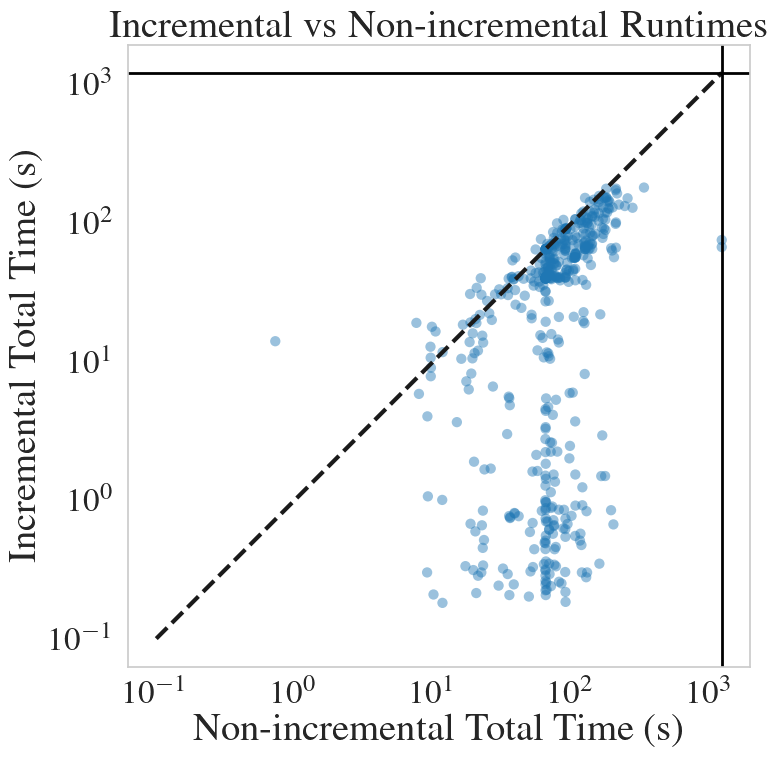
Figure 3 presents a visual comparison of runtimes for both methods on a logarithmic scale. Each point corresponds to a single verification query. Most points lie below the equal-performance line, indicating that incremental verification outperforms the non-incremental baseline on the majority of queries.

4.3 Use Case 3: Minimal Sufficient Feature Set Extraction

Minimal sufficient feature set extraction addresses the problem of explaining a neural network’s prediction by identifying a smallest subset of input features whose values alone suffice to determine the output [43, 42, 8, 29, 12].

Given a reference input and its predicted class, the goal is to identify a subset of input indices such that fixing these features to their reference values guarantees preservation of the predicted class, regardless of how the remaining features vary. While this notion naturally extends to regression settings via a tolerance on the output, we focus here on classification for clarity.

Formally, we seek a feature subset that is sufficient for preserving the prediction and minimal with respect to set inclusion, subject to a given time budget. In this work, unfixed features are allowed to vary freely over their entire domain.

Definition 4(Minimal Sufficient Feature Set)

Let $f:\mathbb{R}^{n}\rightarrow\mathbb{R}^{m}$ be a neural network, $x_{0}\in\mathbb{R}^{n}$ a reference input, and $c=\arg\max_{j}f_{j}(x_{0})$ the predicted class at $x_{0}$. For a subset of feature indices $S\subseteq\{1,\dots,n\}$, define

$$\mathcal{X}_{S}\;=\;\left\{x\in\mathbb{R}^{n}\;\middle|\;x_{i}=(x_{0})_{i}\;\text{for all}\;i\in S\right\}.$$

The set $S$ is a sufficient feature set if

$$\forall x\in\mathcal{X}_{S},\quad\arg\max_{j}f_{j}(x)=c.$$

It is minimal if no strict subset $S^{\prime}\subset S$ is sufficient.

Minimal sufficient feature sets reveal which input features are essential for a given prediction and form a central primitive in formal explainability.

A common approach to solving this task is to search over subsets of input features while invoking a neural network verifier as a subroutine. The procedure begins with all features fixed to their values in the reference input

Figure 4: Minimal sufficient feature set visualizations for GTSRB inputs. Pixels not included in the explanation are shown in gray.

and progressively frees features to test whether preservation of the predicted class is maintained. At a high level, the procedure alternates between proposing candidate feature sets to free and using verification outcomes to determine whether these features can be freed or must remain fixed. This process follows an anytime paradigm: if interrupted due to a timeout, it returns the smallest sufficient feature set identified so far.

To explore the space of feature subsets efficiently, an importance ordering over features is typically computed in a preprocessing step and used to guide a binary-search-style exploration. Rather than freeing features individually, the procedure considers groups of features—often starting from the least important ones—and recursively refines them. Candidate sets are tentatively freed and checked for sufficiency; depending on the outcome, features are either permanently freed or selectively reinstated.

A precise procedural description of this workflow, including the technical modifications required to support incremental verification and the binary-search strategies employed, is provided in Appendix 0.E.3.

Under this formulation, the task gives rise to a collection of verification queries, all defined over the same neural network $f$ and reference input $x_{0}$. Each query $q$ is parameterized by a candidate set of freed features $\overline{S}$, inducing the fixed feature set $S=\{1,\dots,n\}\setminus\overline{S}$ and the corresponding constrained input set $\mathcal{X}_{S}$. The query asks whether fixing all features in $S$ to their values in $x_{0}$ is sufficient to preserve the predicted class $c$. A query returning UNSAT certifies that $S$ is sufficient and that all features in $\overline{S}$ can be freed. In contrast, a SAT result indicates that $S$ is insufficient and that additional features must be fixed. For soundness, TIMEOUT outcomes are treated as SAT.

All queries share the same network $f$, reference input $x_{0}$, and target class $c$; the only varying component is the set of fixed features. As a result, minimal sufficient feature set extraction induces a family of closely related verification queries whose input constraints differ only in which features are fixed.

Due to the binary-search-style exploration, the verification queries generated during minimal sufficient feature set extraction are naturally organized as a search tree rather than a linear sequence. Queries generated after a SAT or TIMEOUT outcome impose strictly stronger input constraints by fixing additional features. In contrast, queries generated after a UNSAT outcome test disjoint sets of features and are therefore incomparable under refinement. Consequently, the overall query family is not totally ordered by refinement.

We formalize the refinement relationship that arises along SAT and TIMEOUT branches of the search tree below.

Proposition 3(Feature-Set Query Refinement)

Let $q$ and $q^{\prime}$ be two verification queries generated during the feature set extraction procedure, corresponding to fixed feature sets $S$ and $S^{\prime}$, respectively. If $q^{\prime}$ is generated from $q$ following a SAT or TIMEOUT outcome, then $S\subset S^{\prime}$ and $q^{\prime}$ is a refinement of $q$, denoted $q^{\prime}\preceq q$.

Proposition 3 shows that, although the full set of queries is not totally ordered, all queries along SAT and TIMEOUT branches form refinement chains. The proof is provided in Appendix 0.D.

Accordingly, in the incremental minimal sufficient feature set extraction procedure, each query $q^{\prime}$ generated after a SAT or TIMEOUT outcome inherits all conflicts learned from its ancestor queries along the same search-tree branch.

4.3.1 Evaluation

We evaluated the effectiveness of incremental conflict reuse for accelerating minimal sufficient feature set extraction on the German Traffic Sign Recognition Benchmark (GTSRB) dataset [32], using a convolutional neural network model from Wu et al. [42]. Out of the $1000$ test inputs considered, $70$ triggered conflicts during SAT or TIMEOUT verification outcomes; the remaining inputs were resolved without conflicts and therefore could not benefit from conflict reuse. We restrict our evaluation to these $70$ cases.

For each input, we ran an anytime minimal sufficient feature set extraction procedure and compared our incremental approach against a non-incremental baseline. Table 3 summarizes the results. The Explanation Size column reports the average size of the minimal sufficient feature set returned within the time budget. Propagations reports the average number of propagations induced by inherited conflicts per task, and Conflicts reports the average number of conflict clauses recorded per task. Both approaches achieve comparable explanation sizes, with the incremental method yielding slightly smaller explanations on average. On average, the incremental approach records $92$ conflicts per task, which induce approximately $2$ effective propagations per task.

Method	Explanation Size	Propagations	Conflicts
Non-incremental	848.52	–	–
Incremental	844.21	2.30	92.14

Table 3: Minimal sufficient feature set extraction on GTSRB.

The primary benefit of incremental verification in this setting lies in its anytime behavior. As shown in Figure 5, incremental verification progressively outperforms the non-incremental baseline in reducing explanation size over time. During the initial phase (up to approximately 20 seconds), both methods exhibit similar performance, with the non-incremental approach sometimes slightly ahead, reflecting the overhead incurred while recording conflicts early in the search.

Figure 5: Incremental vs. non-incremental explanation size over time.

Beyond this point, incremental verification tends to achieve smaller explanations more quickly by reusing previously learned conflicts accumulated earlier in the search. This reuse supports earlier identification of critical features and more efficient pruning of infeasible feature combinations, leading to improved anytime behavior. Overall, these observations suggest that conflict reuse can be beneficial for explainability tasks under an anytime verification regime.

4.4 Results Discussion

We evaluated incremental conflict reuse on three verification tasks: robustness radius determination, input splitting, and minimal sufficient feature set extraction.

In robustness radius determination, queries form a refinement chain, allowing conflicts learned at larger radii to be reused in subsequent queries. This yields a 26% reduction in average verification time compared to the non-incremental baseline (from 315.6 to 233.5 seconds), corresponding to a $1.35\times$ speedup. In input splitting, queries form refinement chains along recursive split branches, allowing conflicts learned in parent subproblems to be reused consistently in descendant queries. This yields a 47% reduction in average verification time compared to the non-incremental baseline (from 84.1 to 43.9 seconds), corresponding to a $1.92\times$ speedup. For minimal sufficient feature set extraction, conflict reuse occurs along refinement chains induced by SAT and TIMEOUT outcomes. While final explanation size improvement is small, incremental reuse improves anytime behavior by reducing explanation size more quickly.

Overall, the impact of incremental conflict reuse is closely tied to the refinement structure of the query family: stronger refinement relations enable greater reuse and larger performance gains.

5 Related Work

Incremental SAT and SMT solving address scalability by reusing learned information, such as conflict clauses and theory lemmas, across sequences of related problem instances [16, 6, 14]. When successive instances are structurally similar, this can avoid redundant reasoning and improve performance. But, the effectiveness of incremental techniques is strongly problem-dependent, and worst-case results in areas such as dynamic graph algorithms show that substantial recomputation may be unavoidable under general updates [21]. Despite the maturity of incremental SAT/SMT solving, its systematic application to neural network verification remains limited.

Prior work on incremental neural network verification has largely focused on settings in which the network itself changes across queries. Residual reasoning [17] reuses information learned for abstract networks to accelerate verification after refinement, while IVAN and I-IVAN [34, 36] reuse successful case splits heuristically across related network architectures. More recently, Zhang et al. [45] study incremental verification guided by counterexample potentiality, again in scenarios where the network is modified.

Related ideas have been explored in abstract interpretation. FANC [37] employs heuristic transfer of abstract bounds to certify multiple approximate neural networks, whereas we reuse conflict information across verification queries on a fixed network.

In contrast, we consider iterative verification over a fixed neural network, where properties or input constraints vary across queries. Our approach reuses learned conflict clauses and provides conditions under which they can be transferred soundly between related verification queries, aligning with conflict-based incremental SAT/SMT solving applied to a single network.

In our evaluation, we instantiated our approach with the CaDiCaL SAT solver [9] and the Marabou verifier [26, 40] as backends. CaDiCaL is a modern SAT solver with a clean design that facilitates its integration with other tools. Marabou is a proof-producing DNN analysis framework [22], which has been used for a myriad of applications, including network pruning [27], formal explainability [7], verifying network generalization [1], and network ensembles [2]. While our implementation relies on Marabou and CaDiCaL, the proposed technique is solver-agnostic and can, in principle, be integrated with other SAT solvers and branch-and-bound verifiers.

6 Limitations and Future Work

The current implementation records conflicts without requiring minimality. As a result, a conflict may include ReLU phase decisions that are not strictly necessary to establish infeasibility. While smaller or subsumed conflicts could improve reuse effectiveness and reduce the overhead of SAT-based reasoning, computing minimal conflicts would require additional analysis and is left for future work [23, 48, 46].

More generally, the approach focuses on reusing conflicts derived from infeasible subproblems. Other reusable information, such as richer theory-specific lemmas or abstractions, may further improve performance in some settings. Exploring such mechanisms would require careful consideration of both soundness and solver integration.

Finally, learned conflicts are used solely for pruning and propagation. An additional direction is to exploit conflicts to guide branching decisions, for example by prioritizing frequently occurring case splits.

7 Conclusion

We introduced an incremental verification approach for neural networks that reuses learned conflict clauses across related verification queries over a fixed network. By formalizing a refinement relation between queries, we showed when such conflicts can be reused soundly and integrated this mechanism into the Marabou verifier as a lightweight extension to branch-and-bound search. Our evaluation shows that conflict reuse reduces redundant exploration and yields speedups of up to $1.9\times$ on representative iterative verification tasks, while preserving soundness.

Appendix

Appendix 0.A Additional Implementation Details

0.A.0.1 Push-Pop of Input and Output Constraints.

To improve efficiency, we introduce a push-pop mechanism for managing input and output constraints in Marabou. This mechanism enables reuse of the encoded neural network and constraints across verification queries by allowing constraints to be incrementally added and removed without re-encoding the network, the constraints, or re-initializing the solver. Using push, the verifier can lock a set of constraints and incrementally add additional ones; a subsequent pop restores the solver state to the previous configuration.

Appendix 0.B Soundness of Conflict Reuse

This appendix contains the proofs of Lemma 1 and Theorem 3.1 from Section 3.

0.B.1 Proof of Lemma 1

Proof

Assume for contradiction that $q_{2}\land\ell_{1}\land\cdots\land\ell_{k}$ is feasible, and let $x$ be a satisfying input. Since $q_{2}\preceq q_{1}$, both queries are defined over the same network $f$, $\mathcal{X}(q_{2})\subseteq\mathcal{X}(q_{1})$, and the ReLU phase literals $\ell_{1},\ldots,\ell_{k}$ refer to the same ReLU constraints in both queries. Therefore, the same input $x$ satisfies $q_{1}\land\ell_{1}\land\cdots\land\ell_{k}$, contradicting infeasibility. ∎

0.B.2 Proof of Theorem 3.1

Proof

Let $c=\{\ell_{1},\ldots,\ell_{k}\}$ be a conflict clause for $q_{1}$. By Definition 1, the subproblem $q_{1}\land\ell_{1}\land\cdots\land\ell_{k}$ is infeasible. Since $q_{2}\preceq q_{1}$, infeasibility is monotone under refinement by Lemma 1. Therefore, the subproblem $q_{2}\land\ell_{1}\land\cdots\land\ell_{k}$ is also infeasible, and hence $c$ is a conflict clause for $q_{2}$. ∎

Appendix 0.C Soundness of SAT-Based Conflict Reasoning

This appendix provides proofs for Lemmas 2 and 3, which establish the soundness of SAT-based pruning and propagation using learned conflict clauses.

0.C.1 Proof of Lemma 2

Proof

Suppose, for contradiction, that there exists a feasible solution for query $q$ that extends the partial assignment $\alpha$. Then there exists a complete assignment that satisfies all literals in $\alpha$ and corresponds to a feasible input for $q$.

Since the propositional CNF formula constructed from $\alpha$ and the clauses in $\mathcal{C}$ is UNSAT, every complete assignment extending $\alpha$ must violate at least one conflict clause $c\in\mathcal{C}$. By Definition 1, each conflict clause forbids the simultaneous satisfaction of all its literals, and any assignment violating $c$ cannot correspond to a feasible solution for $q$. This contradicts the assumption of feasibility. Therefore, no extension of $\alpha$ can correspond to a feasible solution for $q$. ∎

0.C.2 Proof of Lemma 3

Proof

Let $\mathcal{L}$ be the set of literals implied by unit propagation when solving the SAT instance under assumptions $\alpha$. By definition of unit propagation, for each $\ell\in\mathcal{L}$, assigning $\neg\ell$ under $\alpha$ would falsify at least one conflict clause $c\in\mathcal{C}$.

Suppose, for contradiction, that there exists a feasible solution for $q$ that extends $\alpha$ but violates some implied literal $\ell\in\mathcal{L}$. Then the corresponding complete assignment satisfies $\alpha\cup\{\neg\ell\}$ and therefore violates the conflict clause $c$. By Definition 1, this assignment cannot correspond to a feasible solution for $q$, contradicting feasibility.

Hence, every feasible extension of $\alpha$ must satisfy all literals in $\mathcal{L}$. ∎

Appendix 0.D Proofs of Refinement Properties of Verification Use Cases

This appendix provides proofs of the refinement properties for the verification use cases discussed in Section 4.

0.D.1 Proof of Proposition 1

Proof

The two queries are defined over the same network $f$ and reference input $x_{0}$. The input constraints of the two queries are given by

$$\mathcal{X}(q_{i})\;=\;\left\{x\in\mathbb{R}^{n}\;\middle|\;\|x-x_{0}\|\leq\varepsilon_{i}\right\},\quad\mathcal{X}(q_{j})\;=\;\left\{x\in\mathbb{R}^{n}\;\middle|\;\|x-x_{0}\|\leq\varepsilon_{j}\right\}.$$

Since $\varepsilon_{j}<\varepsilon_{i}$, it follows immediately that $\mathcal{X}(q_{j})\subseteq\mathcal{X}(q_{i})$. The output constraints of both queries are identical, as they are defined by the same predicate $\mathcal{P}(x_{0},x)$. Therefore, by Definition 2, $q_{j}$ is a refinement of $q_{i}$. ∎

0.D.2 Proof of Proposition 2

Proof

Let $q_{0}$ be a verification query, and let $q_{1}$ be a verification query generated by input splitting of $q_{0}$. By construction, input splitting partitions the input domain of $q_{0}$ into subregions, and thus the input domain of $q_{1}$ is a subset of that of $q_{0}$, i.e., $\mathcal{X}(q_{1})\subseteq\mathcal{X}(q_{0}).$ Moreover, input splitting does not modify the network or the output constraints. Hence, $\mathcal{Y}(q_{1})=\mathcal{Y}(q_{0})$, and in particular $\mathcal{Y}(q_{1})\subseteq\mathcal{Y}(q_{0})$. Therefore, by Definition 2, $q_{1}$ is a refinement of $q_{0}$. ∎

0.D.3 Proof of Proposition 3

Proof

By construction, a successor query $q^{\prime}$ generated after a SAT or TIMEOUT outcome is obtained by reinstating a subset of previously freed features. Thus, the corresponding fixed feature sets satisfy $S\subset S^{\prime}$.

The input constraints of the two queries are given by

$$\mathcal{X}_{S}=\left\{x\in\mathbb{R}^{n}\;\middle|\;x_{i}=(x_{0})_{i}\;\text{for all}\;i\in S\right\},\\ \mathcal{X}_{S^{\prime}}=\left\{x\in\mathbb{R}^{n}\;\middle|\;x_{i}=(x_{0})_{i}\;\text{for all}\;i\in S^{\prime}\right\}.$$

Since $S\subset S^{\prime}$, it follows that $\mathcal{X}_{S^{\prime}}\subseteq\mathcal{X}_{S}$.

Both queries enforce the same output constraint, namely preservation of the predicted class $c$. Therefore, by Definition 2, $q^{\prime}$ is a refinement of $q$. ∎

Appendix 0.E Algorithmic Details and Pseudocodes

0.E.1 Robustness Radius Interval Computation

This appendix provides pseudocode and a description of the robustness radius interval computation used in Section 4.1. We present the algorithmic workflow by which lower and upper bounds on the local robustness radius are iteratively refined through repeated verification queries until the desired precision is achieved or the time budget is exhausted. In addition, we highlight the modifications required to enable incremental reuse of learned conflicts across related verification queries.

Input: Reference input $x_{0}$; initial interval $[\varepsilon_{\min},\varepsilon_{\max}]$; precision $\delta>0$; time budget $T$; verification subroutine $\textsc{Verify}(\varepsilon)$ with optional incremental reuse of inherited conflicts

Output: Certified bounds $(\underline{\varepsilon},\overline{\varepsilon})$ such that $\underline{\varepsilon}\leq\varepsilon^{\star}\leq\overline{\varepsilon}$ and $\overline{\varepsilon}-\underline{\varepsilon}\leq\delta$ if completed within $T$.

1

2Interface: $\textsc{Verify}(\varepsilon,x_{0})$ returns $(res,x_{\text{ce}})$ where $res\in\{\textsf{UNSAT},\textsf{SAT},\textsf{TIMEOUT}\}$ and $x_{\text{ce}}\neq\bot$ only if $res=\textsf{SAT}$. In incremental mode, we call $\textsc{Verify}(\varepsilon,x_{0},id,\mathcal{I})$ where $id$ is the query identifier and $\mathcal{I}$ is a set of inherited query identifiers.

3

41ex

5$start\leftarrow\textsc{Now}()$

6

7$\underline{\varepsilon}\leftarrow\varepsilon_{\min}$,   $\overline{\varepsilon}\leftarrow\varepsilon_{\max}$

8 $stepRatio\leftarrow 1/2$,   $direction\leftarrow\textsf{down}$

9

$nextId\leftarrow 0$

// counter for verification-query identifiers

10

11while $(\overline{\varepsilon}-\underline{\varepsilon})>\delta$ and $\textsc{Now}()-start<T$ do

12    $w\leftarrow\overline{\varepsilon}-\underline{\varepsilon}$

13    if $direction=\textsf{down}$ then

14       $\varepsilon\leftarrow\overline{\varepsilon}-stepRatio\cdot w$

15      

16   else

17       $\varepsilon\leftarrow\underline{\varepsilon}+stepRatio\cdot w$

18      

19   

20   $id\leftarrow nextId;\;\;nextId\leftarrow nextId+1$

21    $\varepsilon_{id}\leftarrow\varepsilon$

22   

23   $\mathcal{I}\leftarrow\{\,id^{\prime}\mid id^{\prime}\text{ was issued earlier with }\varepsilon_{id^{\prime}}>\varepsilon\,\}$

    $res,\;x_{\text{ce}}\leftarrow\textsc{Verify}(\varepsilon,x_{0}{\color[rgb]{0,0,1}\definecolor[named]{pgfstrokecolor}{rgb}{0,0,1},\,id,\,\mathcal{I}})$

    // $x_{\text{ce}}$ is returned only if $res=\textsf{SAT}$

24   

25   if $res=\textsf{UNSAT}$ then

26       $\underline{\varepsilon}\leftarrow\varepsilon$

27       $stepRatio\leftarrow 1/2$; $direction\leftarrow\textsf{down}$

28      

29    else if $res=\textsf{SAT}$ then

       $\overline{\varepsilon}\leftarrow\|x_{\text{ce}}-x_{0}\|_{\infty}$

       // counterexample might yield a tighter bound

30       $stepRatio\leftarrow 1/2$; $direction\leftarrow\textsf{down}$

31      

32    else // TIMEOUT

33       if $direction=\textsf{down}$ then

34          $stepRatio\leftarrow stepRatio/2$

35          $direction\leftarrow\textsf{up}$

36         

37      else

38          $direction\leftarrow\textsf{down}$

39         

40      

41   

42

43return $\underline{\varepsilon},\overline{\varepsilon}$

Algorithm 3 Robustness Radius Interval Computation with Incremental Reuse

Given a neural network $f:\mathbb{R}^{n}\rightarrow\mathbb{R}^{m}$, a reference input $x_{0}\in\mathbb{R}^{n}$, and an output consistency predicate $\mathcal{P}(x_{0},x)$, the objective is to compute certified lower and upper bounds $\underline{\varepsilon}$ and $\overline{\varepsilon}$ on the local robustness radius $\varepsilon^{\star}$ at $x_{0}$, up to a prescribed precision $\delta>0$ and within a time budget $T$.

The procedure is presented in Algorithm 3. It relies on a verification subroutine $\textsc{Verify}(...)$ that, given a perturbation radius $\varepsilon$ and the reference input $x_{0}$, determines whether the property $\mathcal{P}(x_{0},x)$ holds for all inputs $x$ satisfying $\|x-x_{0}\|_{\infty}\leq\varepsilon$. In other words, it returns one of three possible outcomes: UNSAT, SAT, or TIMEOUT. In non-incremental mode, the call takes only the parameters $\varepsilon$ and $x_{0}$ as input: $\textsc{Verify}(\varepsilon,x_{0})$. In incremental mode, the call $\textsc{Verify}(\varepsilon,x_{0}{\color[rgb]{0,0,1}\definecolor[named]{pgfstrokecolor}{rgb}{0,0,1},\,id,\,\mathcal{I}})$ additionally takes a unique query identifier $id$ and a set of inherited query identifiers $\mathcal{I}$, enabling reuse of learned conflicts. The elements related to incremental reuse are highlighted in blue in the algorithm.

The algorithm assumes the initial bracketing interval $[\varepsilon_{\min},\varepsilon_{\max}]$ is valid (i.e. $\textsc{Verify}(\varepsilon_{\min},x_{0})$ returns UNSAT, and $\textsc{Verify}(\varepsilon_{\max},x_{0})$ returns SAT). After initializing the time budget and bounds (Lines 3–3), the procedure iteratively refines the current interval $[\underline{\varepsilon},\overline{\varepsilon}]$ within a main loop (Line 3).

In each iteration, a candidate perturbation radius $\varepsilon$ is selected from the current interval and issued as a verification query. In incremental mode, the query is assigned a fresh identifier and augmented with a set of inherited identifiers corresponding to earlier queries at larger radii (Line 3). The verification subroutine is then invoked (Line 3).

The outcome of the verification determines how the interval is updated. If the result is UNSAT, robustness is certified at radius $\varepsilon$ and the lower bound $\underline{\varepsilon}$ is raised accordingly (Line 3). If the result is SAT, a counterexample is returned and used to tighten the upper bound $\overline{\varepsilon}$ based on its distance from $x_{0}$ (Line 3). If the verification attempt times out, the algorithm conservatively adapts its search direction and step size without updating the bounds (Line 3).

The procedure terminates once the interval width $\overline{\varepsilon}-\underline{\varepsilon}$ falls below the target precision $\delta$, or when the available time budget is exhausted. The final bounds $(\underline{\varepsilon},\overline{\varepsilon})$ are then returned (Line 3).

0.E.2 Input-Split Verification with Incremental Reuse

This appendix provides pseudocode and a description of the input-split verification procedure used for neural network properties in Section 4.2. We present the algorithmic workflow by which the input space is recursively partitioned when verification queries time out, enabling the solver to make progress on difficult instances. In addition, we highlight the modifications required to enable incremental reuse of learned conflicts across related verification queries.

Input: Neural network $f:\mathbb{R}^{n}\rightarrow\mathbb{R}^{m}$; property $\phi$; initial timeout $T_{0}$; timeout factor $\alpha$; verification subroutine $\textsc{Verify}(\mathcal{Q},T)$ with optional incremental reuse of inherited conflicts

Output: Verification result: $res\in\{\textsf{UNSAT},\textsf{SAT},\textsf{TIMEOUT}\}$.

1

2Interface: $\textsc{Verify}(\mathcal{Q},T)$ returns $res\in\{\textsf{UNSAT},\textsf{SAT},\textsf{TIMEOUT}\}$ where $\mathcal{Q}$ is a verification query with input bounds and $T$ is the timeout. In incremental mode, we call $\textsc{Verify}(\mathcal{Q},T,id,\mathcal{I})$ where $id$ is a query identifier and $\mathcal{I}$ is a set of inherited (ancestor) query identifiers.

3

41ex

$nextId\leftarrow 0$

// counter for query identifiers

$\mathcal{Q}_{0}\leftarrow\textsc{ConstructQuery}(f,\phi)$

// initial query

5 return $\textsc{InputSplitSearch}(\mathcal{Q}_{0},T_{0}{\color[rgb]{0,0,1}\definecolor[named]{pgfstrokecolor}{rgb}{0,0,1},\,\emptyset})$

6

7Function $\textsc{InputSplitSearch}(\mathcal{Q},T{\color[rgb]{0,0,1}\definecolor[named]{pgfstrokecolor}{rgb}{0,0,1},\,\mathcal{I}})$

8    $id\leftarrow nextId;\;\;nextId\leftarrow nextId+1$

9    $res\leftarrow\textsc{Verify}(\mathcal{Q},T{\color[rgb]{0,0,1}\definecolor[named]{pgfstrokecolor}{rgb}{0,0,1},\,id,\,\mathcal{I}})$

10   

11   if $res=\textsf{SAT}$ or $res=\textsf{UNSAT}$ then

12       return $res$

13      

14   

15   $v\leftarrow\textsc{SelectWidestInput}(\mathcal{Q})$

16   

17   $[\ell,u]\leftarrow\textsc{GetBounds}(\mathcal{Q},v)$

18    $m\leftarrow(\ell+u)/2$

    $\mathcal{I}^{\prime}\leftarrow\mathcal{I}\cup\{id\}$

    // inherit from parent

19   

20   $\mathcal{Q}_{L}\leftarrow\textsc{TightenUpper}(\mathcal{Q},v,m)$

21    $res_{L}\leftarrow\textsc{InputSplitSearch}(\mathcal{Q}_{L},\alpha\cdot T{\color[rgb]{0,0,1}\definecolor[named]{pgfstrokecolor}{rgb}{0,0,1},\,\mathcal{I}^{\prime}})$

22   

23   if $res_{L}=\textsf{SAT}$ then

24       return SAT

25      

26   

27   $\mathcal{Q}_{R}\leftarrow\textsc{TightenLower}(\mathcal{Q},v,m)$

28    $res_{R}\leftarrow\textsc{InputSplitSearch}(\mathcal{Q}_{R},\alpha\cdot T{\color[rgb]{0,0,1}\definecolor[named]{pgfstrokecolor}{rgb}{0,0,1},\,\mathcal{I}^{\prime}})$

29   

30   if $res_{R}=\textsf{SAT}$ then

31       return SAT

32      

33   

34   if $res_{L}=\textsf{UNSAT}$ and $res_{R}=\textsf{UNSAT}$ then

35       return UNSAT

36      

37    else

38       return TIMEOUT

39      

40   

Algorithm 4 Input-Split Verification with Incremental Reuse

Given a neural network $f:\mathbb{R}^{n}\rightarrow\mathbb{R}^{m}$, a property $\phi$ to verify, the objective is to determine whether the property holds over the input space. The procedure is presented in Algorithm 4. As in the previous use case, it relies on a verification subroutine $\textsc{Verify}(...)$ that, given a verification query $\mathcal{Q}$ with input bounds and a timeout $T$, determines whether the property holds for all inputs in the constrained space. In other words, it returns one of three possible outcomes: UNSAT, SAT, or TIMEOUT. In non-incremental mode, the call takes only the parameters $\mathcal{Q}$ and $T$ as input: $\textsc{Verify}(\mathcal{Q},T)$. In incremental mode, the call $\textsc{Verify}(\mathcal{Q},T{\color[rgb]{0,0,1}\definecolor[named]{pgfstrokecolor}{rgb}{0,0,1},\,id,\,\mathcal{I}})$ additionally takes a unique query identifier $id$ and a set of inherited query identifiers $\mathcal{I}$, enabling reuse of learned conflicts. The elements related to incremental reuse are highlighted in blue in the algorithm.

The algorithm constructs an initial verification query $\mathcal{Q}_{0}$ from the network $f$ and property $\phi$, then invokes the recursive search procedure InputSplitSearch. At each node, the algorithm attempts to verify the current query $\mathcal{Q}$ with timeout $T$ (Line 4). In incremental mode, the query is assigned a fresh identifier and augmented with a set of inherited identifiers from ancestor queries. If the verification returns a conclusive result (SAT or UNSAT), that result is immediately returned (Line 4).

When verification times out, the algorithm selects the input variable with the widest valid range (Line 4) and splits its domain at the midpoint, creating two disjoint subspaces. The parent query’s identifier is added to the inherited set $\mathcal{I}^{\prime}$ for child queries, enabling conflict reuse.

Two subproblems are created by tightening the upper bound (Line 4) and lower bound (Line 4) of the selected input variable. Each recursive call uses increased timeout $\alpha\cdot T$. If either branch finds a counterexample (SAT), the query returns SAT (Lines 4, 4). If the UNSAT partitions collectively cover the entire input space, the query is UNSAT (Line 4). Otherwise, the result is TIMEOUT (Line 4).

0.E.3 Minimal Sufficient Feature Set Extraction: Binary-Sequential Procedure

This appendix provides pseudocode and a description of the recursive binary search workflow used in Section 4.3. The procedure repeatedly invokes a verification subroutine to determine whether a candidate set of features can be freed while preserving the reference prediction. The underlying binary search strategy follows [42] and is adapted here to support incremental reuse of learned conflicts across related verification queries, which arise along SAT and TIMEOUT branches of the search.

Input: Neural network $f$; reference input $x_{0}\in\mathbb{R}^{n}$; target class $c=\arg\max_{j}f_{j}(x_{0})$; feature universe $U=\{1,\dots,n\}$; verification subroutine $\textsc{Verify}(\overline{S})$ with optional incremental reuse of inherited conflicts.

Output: feature set that must remain fixed ($S_{\text{fixed}}$), feature set certified freeable ($S_{\text{freed}}$).

1

2Interface: $\textsc{Verify}(\overline{S},x_{0})$ returns $res\in\{\textsf{UNSAT},\textsf{SAT},\textsf{TIMEOUT}\}$ and verifies if $U\setminus\overline{S}$ is a sufficient feature set for $x_{0}$. In incremental mode, we call $\textsc{Verify}(\overline{S},x_{0},id,\mathcal{I})$ where $id$ is a query identifier and $\mathcal{I}$ is a set of inherited (ancestor) query identifiers.

3

41ex

5$S_{\text{fixed}}\leftarrow\emptyset$; $S_{\text{freed}}\leftarrow\emptyset$

$nextId\leftarrow 0$

// counter for query identifiers

6

7$\textsc{BinaryMinimalSufficiencySearch}(U,{\color[rgb]{0,0,1}\definecolor[named]{pgfstrokecolor}{rgb}{0,0,1}\emptyset})$

8 return $S_{\text{fixed}},S_{\text{freed}}$

9

10Function $\textsc{BinaryMinimalSufficiencySearch}(S_{\text{cand}},{\color[rgb]{0,0,1}\definecolor[named]{pgfstrokecolor}{rgb}{0,0,1}\mathcal{I}})$

11    if $|S_{\text{cand}}|=1$ then

12       $id\leftarrow nextId;\;\;nextId\leftarrow nextId+1$

13       $res\leftarrow\textsc{Verify}(S_{\text{freed}}\cup S_{\text{cand}},x_{0}{\color[rgb]{0,0,1}\definecolor[named]{pgfstrokecolor}{rgb}{0,0,1},\,id,\,\mathcal{I}})$

14       if $res=\textsf{UNSAT}$ then

15          $S_{\text{freed}}\leftarrow S_{\text{freed}}\cup S_{\text{cand}}$

16         

17       else // SAT or TIMEOUT

18          $S_{\text{fixed}}\leftarrow S_{\text{fixed}}\cup S_{\text{cand}}$

19         

20      return

21      

22   

23   $(S_{\text{left}},S_{\text{right}})\leftarrow\textsc{Split}(S_{\text{cand}})$

24    $id_{\text{left}}\leftarrow nextId;\;\;nextId\leftarrow nextId+1$

25    $res_{\text{left}}\leftarrow\textsc{Verify}(S_{\text{freed}}\cup S_{\text{left}},x_{0}{\color[rgb]{0,0,1}\definecolor[named]{pgfstrokecolor}{rgb}{0,0,1},\,id_{\text{left}},\,\mathcal{I}})$

26   

27   if $res_{\text{left}}=\textsf{UNSAT}$ then

28       $S_{\text{freed}}\leftarrow S_{\text{freed}}\cup S_{\text{left}}$

29      

30      $id_{\text{right}}\leftarrow nextId;\;\;nextId\leftarrow nextId+1$

31       $res_{\text{right}}\leftarrow\textsc{Verify}(S_{\text{freed}}\cup S_{\text{right}},x_{0}{\color[rgb]{0,0,1}\definecolor[named]{pgfstrokecolor}{rgb}{0,0,1},\,id_{\text{right}},\,\mathcal{I}})$

32      

33      if $res_{\text{right}}=\textsf{UNSAT}$ then

34          $S_{\text{freed}}\leftarrow S_{\text{freed}}\cup S_{\text{right}}$

35         

36       else // SAT or TIMEOUT

37          $\textsc{BinaryMinimalSufficiencySearch}(S_{\text{right}},{\color[rgb]{0,0,1}\definecolor[named]{pgfstrokecolor}{rgb}{0,0,1}\mathcal{I}\cup\{id_{\text{right}}\}})$

38         

39      

40    else // SAT or TIMEOUT

41      

42      if $|S_{\text{left}}|=1$ then

43          $S_{\text{fixed}}\leftarrow S_{\text{fixed}}\cup S_{\text{cand}}$

44         

45       else

46          $\textsc{BinaryMinimalSufficiencySearch}(S_{\text{left}},{\color[rgb]{0,0,1}\definecolor[named]{pgfstrokecolor}{rgb}{0,0,1}\mathcal{I}\cup\{id_{\text{left}}\}})$

47         

48      $\textsc{BinaryMinimalSufficiencySearch}(S_{\text{right}})$

49      

50   

Algorithm 5 Minimal Sufficient Feature Set Extraction with Incremental Reuse

Given a neural network $f:\mathbb{R}^{n}\rightarrow\mathbb{R}^{m}$ and a reference input $x_{0}\in\mathbb{R}^{n}$, the goal is to extract a minimal sufficient feature set for the predicted class $c=\arg\max_{j}f_{j}(x_{0})$. Equivalently, the goal is to partition the feature universe $U=\{1,\dots,n\}$ into two disjoint sets: $S_{\text{fixed}}$, the set of features that must remain fixed to their values in $x_{0}$, and $S_{\text{freed}}$, the set of features certified freeable, such that fixing $S_{\text{fixed}}$ suffices to preserve the prediction under arbitrary assignments to the features in $S_{\text{freed}}$.

The procedure is presented in Algorithm 5. It relies on a verification subroutine $\textsc{Verify}(...)$ that, given a set of candidate features $\overline{S}$ to free, determines whether $U\setminus\overline{S}$ constitutes a sufficient feature set for $x_{0}$. In other words, it returns one of three possible outcomes: UNSAT, SAT, or TIMEOUT. In non-incremental mode, the call takes only the parameters $\overline{S}$ and $x_{0}$ as input: $\textsc{Verify}(\overline{S},x_{0})$. In incremental mode, the call $\textsc{Verify}(\overline{S},x_{0}{\color[rgb]{0,0,1}\definecolor[named]{pgfstrokecolor}{rgb}{0,0,1},\,id,\,\mathcal{I}})$ additionally takes a unique query identifier $id$ and a set of inherited query identifiers $\mathcal{I}$, enabling reuse of learned conflicts. The elements related to incremental reuse are highlighted in blue in the algorithm.

Algorithm 5 maintains the evolving sets $S_{\text{fixed}}$ and $S_{\text{freed}}$ (Line 5). At each step it processes a candidate set of features $S_{\text{cand}}$ and attempts to certify as many of them as freeable. This is done by invoking the verification subroutine $\textsc{Verify}(S_{\text{freed}}\cup S_{\text{cand}},x_{0})$ (Line 5), which checks whether freeing the proposed features preserves the predicted class $c$ while all remaining features are fixed to their values in $x_{0}$.

An UNSAT result certifies that all features in the proposed set may be freed, and the algorithm adds them to $S_{\text{freed}}$ (Lines 5, 5, and 5). A SAT or TIMEOUT result indicates that the proposed set cannot be freed as a whole, and the algorithm refines the candidate by splitting it into smaller subsets (Line 5) and continuing the search recursively on the subset(s) that remain uncertified.

The recursion terminates at singletons (Lines 5 and 5). If a singleton feature cannot be freed, it is classified as necessary and added to $S_{\text{fixed}}$ (Lines 5 and 5). Otherwise, it is added to $S_{\text{freed}}$ (Line 5). By iteratively certifying freeable groups and isolating necessary singletons, the procedure constructs $S_{\text{fixed}}$ as an explanation whose fixed values suffice to preserve the prediction, while maximizing $S_{\text{freed}}$.

In incremental mode, each call to Verify is issued with a query identifier and a set of inherited identifiers $\mathcal{I}$, representing ancestor queries whose learned conflicts may be reused. As shown in Algorithm 5, inheritance is updated only along branches where the current candidate set is not certified freeable, i.e., on SAT and TIMEOUT outcomes. Concretely, when the verification of a subset fails, the identifier of that query is added to the inherited set passed to the recursive call (Lines 5 and 5). In contrast, UNSAT outcomes certify freeability and do not induce further recursion, and therefore do not require extending the ancestry set.

This design ensures that conflict inheritance is applied along refinement branches, enabling effective reuse while preserving soundness.

References

- [1] (2023) Verifying Generalization in Deep Learning. In Proc. 35th Int. Conf. on Computer Aided Verification (CAV), pp. 438–455. Cited by: §5.
- [2] (2022) Verification-Aided Deep Ensemble Selection. In Proc. 22nd Int. Conf. on Formal Methods in Computer-Aided Design (FMCAD), pp. 27–37. Cited by: §5.
- [3] (2016) Concrete Problems in AI Safety. Note: Technical Report. http://arxiv.org/abs/1606.06565 Cited by: §1.
- [4] (2021) The Second International Verification of Neural Networks Competition (VNN-COMP 2021): Summary and Results. Note: Technical Report. http://arxiv.org/abs/2109.00498 Cited by: §4.1.1.
- [5] (2020) Improved Geometric Path Enumeration for Verifying ReLU Neural Networks. In Proc. 32nd Int. Conf. on Computer Aided Verification (CAV), pp. 66–96. Cited by: §2.2.
- [6] (2018) Satisfiability Modulo Theories. In Handbook of Model Checking, E. M. Clarke, T. A. Henzinger, H. Veith, and R. Bloem (Eds.), pp. 305–343. Cited by: §1, §5.
- [7] (2023) Formally Explaining Neural Networks within Reactive Systems. In Proc. 23rd Int. Conf. on Formal Methods in Computer-Aided Design (FMCAD), pp. 10–22. Cited by: §5.
- [8] (2023) Towards Formal XAI: Formally Approximate Minimal Explanations of Neural Networks. In Proc. 29th Int. Conf. on Tools and Algorithms for the Construction and Analysis of Systems (TACAS), pp. 187–207. Cited by: §1, §4.3.
- [9] (2024) CaDiCaL 2.0. In Proc. 36th Int. Conf. on Computer Aided Verification (CAV), pp. 133–152. Cited by: §4, §5.
- [10] (2016) End to End Learning for Self-Driving Cars. Note: Technical Report. http://arxiv.org/abs/1604.07316 Cited by: §1.
- [11] (2020) Efficient Verification of ReLU-Based Neural Networks via Dependency Analysis. In Proc. 34th AAAI Conf. on Artificial Intelligence (AAAI), pp. 3291–3299. Cited by: §2.2, §2.2.
- [12] (2026) FAME: Formal Abstract Minimal Explanation for neural networks. In Proc. 14th Int. Conf. on Learning Representations (ICLR), Cited by: §1, §4.3.
- [13] (2023) First Three Years of the International Verification of Neural Networks Competition (VNN-COMP). International Journal on Software Tools for Technology Transfer (STTT) 25 (3), pp. 329–339. Cited by: §4.1.1.
- [14] (2008) Z3: An Efficient SMT Solver. In Proc. 14th Int. Conf. on Tools and Algorithms for the Construction and Analysis of Systems (TACAS), pp. 337–340. Cited by: §1, §5.
- [15] (2025) NeuralSAT: A High-Performance Verification Tool for Deep Neural Networks. In Proc. 37th Int. Conf. on Computer Aided Verification (CAV), pp. 409–423. Cited by: §2.2.
- [16] (2004) An Extensible SAT-Solver. In Proc. 7th Int. Conf. on Theory and Applications of Satisfiability Testing (SAT), pp. 502–518. Cited by: §1, §5.
- [17] (2022) Neural Network Verification Using Residual Reasoning. In Proc. 20th Int. Conf. on Software Engineering and Formal Methods (SEFM), pp. 173–189. Cited by: §5.
- [18] (2024) Robustness Assessment of a Runway Object Classifier for Safe Aircraft Taxiing. In Proc. 43rd IEEE/ACM Digital Avionics Systems Conf. (DASC), pp. 1–6. Cited by: §1, §1.
- [19] (2017) Dermatologist-Level Classification of Skin Cancer with Deep Neural Networks. Nature 542 (7639), pp. 115–118. Cited by: §1.
- [20] (2016) Deep Learning. MIT Press. Cited by: §2.1.
- [21] (2001) Poly-Logarithmic Deterministic Fully-Dynamic Algorithms for Connectivity, Minimum Spanning Tree, 2-Edge, and Biconnectivity. Journal of the ACM (JACM) 48 (4), pp. 723–760. Cited by: §5.
- [22] (2022) Neural Network Verification with Proof Production. In Proc. 22nd Int. Conf. on Formal Methods in Computer-Aided Design (FMCAD), pp. 38–48. Cited by: §5.
- [23] (2026) Proof Minimization in Neural Network Verification. In Proc. 27th Int. Conf. on Verification, Model Checking, and Abstract Interpretation (VMCAI), pp. 99–124. Cited by: §6.
- [24] (2017) Reluplex: An Efficient SMT Solver for Verifying Deep Neural Networks. In Proc. 29th Int. Conf. on Computer Aided Verification (CAV), pp. 97–117. Cited by: §1, §1, §1, §2.2, §2.2.
- [25] (2017) Towards Proving the Adversarial Robustness of Deep Neural Networks. In Proc. 1st Workshop on Formal Verification of Autonomous Vehicles (FVAV), pp. 19–26. Cited by: §1.
- [26] (2019) The Marabou Framework for Verification and Analysis of Deep Neural Networks. In Proc. 31st Int. Conf. on Computer Aided Verification (CAV), pp. 443–452. Cited by: §1, §2.2, §2.2, §4, §5.
- [27] (2021) Pruning and Slicing Neural Networks using Formal Verification. In Proc. 21st Int. Conf. on Formal Methods in Computer-Aided Design (FMCAD), pp. 183–192. Cited by: §5.
- [28] (2024) Formally Verifying Deep Reinforcement Learning Controllers with Lyapunov Barrier Certificates. In Proc. 24th Int. Conf. on Formal Methods in Computer-Aided Design (FMCAD), pp. 95–106. Cited by: §4.2.1.
- [29] (2022) Delivering Trustworthy AI through Formal XAI. In Proc. 36th AAAI Conf. on Artificial Intelligence (AAAI), pp. 12342–12350. Cited by: §4.3.
- [30] (2019) Compositional Verification for Autonomous Systems with Deep Learning Components. In Safe, Autonomous and Intelligent Vehicles, H. Yu, X. Li, R. M. Murray, S. Ramesh, and C. J. Tomlin (Eds.), pp. 187–197. Cited by: §1.
- [31] (2019) An Abstract Domain for Certifying Neural Networks. In Proc. 46th ACM SIGPLAN Symposium on Principles of Programming Languages (POPL), Cited by: §2.2.
- [32] (2011) The German Traffic Sign Recognition Benchmark: A Multi-Class Classification Competition. In Proc. IEEE Int. Joint Conf. on Neural Networks (IJCNN), pp. 1453–1460. Cited by: §4.3.1.
- [33] (2023) Global Optimization of Objective Functions Represented by ReLU Networks. Machine Learning 112 (10), pp. 3685–3712. Cited by: §1.
- [34] (2024) Improved Incremental Verification for Neural Networks. In Proc. 18th Int. Conf. on Theoretical Aspects of Software Engineering (TASE), pp. 392–409. Cited by: §1, §5.
- [35] (2020) NNV: The Neural Network Verification Tool for Deep Neural Networks and Learning-Enabled Cyber-Physical Systems. In Proc. 32nd Int. Conf. on Computer Aided Verification (CAV), pp. 3–17. Cited by: §2.2, §2.2.
- [36] (2023) Incremental Verification of Neural Networks. In Proc. 44th ACM SIGPLAN Conf. on Programming Language Design and Implementation (PLDI), Cited by: §1, §5.
- [37] (2022) Proof Transfer for Fast Certification of Multiple Approximate Neural Networks. In Proc. 37th ACM SIGPLAN Conf. on Object-Oriented Programming, Systems, Languages, and Applications (OOPSLA), Cited by: §1, §5.
- [38] (2018) Formal Security Analysis of Neural Networks Using Symbolic Intervals. In Proc. 27th USENIX Security Symposium (USENIX Security), pp. 1599–1614. Cited by: §2.2.
- [39] (2021) Beta-CROWN: Efficient Bound Propagation with Per-Neuron Split Constraints for Complete and Incomplete Neural Network Verification. In Proc. 35th Conf. on Neural Information Processing Systems (NeurIPS), Cited by: §2.2, §2.2.
- [40] (2024) Marabou 2.0: A Versatile Formal Analyzer of Neural Networks. In Proc. 36th Int. Conf. on Computer Aided Verification (CAV), pp. 249–264. Cited by: §1, §4, §5.
- [41] (2020) Parallelization Techniques for Verifying Neural Networks. In Proc. 20th Int. Conf. on Formal Methods in Computer-Aided Design (FMCAD), pp. 128–137. Cited by: §4.2.
- [42] (2025) Efficiently Computing Compact Formal Explanations. Note: Technical Report. http://arxiv.org/abs/2409.03060 Cited by: §0.E.3, §1, §4.3.1, §4.3.
- [43] (2023) VeriX: Towards Verified Explainability of Deep Neural Networks. In Proc. 37th Conf. on Neural Information Processing Systems (NeurIPS), pp. 22247–22268. Cited by: §1, §4.3.
- [44] (2020) Automatic Perturbation Analysis for Scalable Certified Robustness and Beyond. In Proc. 34th Conf. on Neural Information Processing Systems (NeurIPS), Cited by: §2.2.
- [45] (2025) Efficient Incremental Verification of Neural Networks Guided by Counterexample Potentiality. In Proc. 40th ACM SIGPLAN Conf. on Object-Oriented Programming, Systems, Languages, and Applications (OOPSLA), Cited by: §5.
- [46] (2022) General Cutting Planes for Bound-Propagation-Based Neural Network Verification. In Proc. 36th Conf. on Neural Information Processing Systems (NeurIPS), Cited by: §6.
- [47] (2018) Efficient Neural Network Robustness Certification with General Activation Functions. In Proc. 32nd Conf. on Neural Information Processing Systems (NeurIPS), pp. 4939–4948. Cited by: §2.2, §2.2.
- [48] (2024) Scalable Neural Network Verification with Branch-and-Bound Inferred Cutting Planes. In Proc. 38th Conf. on Neural Information Processing Systems (NeurIPS), Cited by: §6.