Analytic Singular Slow-roll Inflation

Abstract

We study a class of minimally coupled scalar field theories which leads to analytic solutions for the Hubble rate and the scalar field. The inflationary phenomenology for this class of models can be studied fully analytically. The resulting phenomenology is compatible with the ACT data and for limiting cases, the spectral index is bluer than the ACT constraints and tends to the value $n_{\mathcal{S}}=0.98$, while in the limiting case, the tensor-to-scalar ratio takes very small values, nearly zero. More importantly, the resulting cosmology describes a Universe that has a finite scale factor at $t=0$, thus non-singular, evolves and expands realizing a slow-roll inflationary era and after that it reaches classically a pressure singularity. Classically, the Universe can pass through this singularity, and a turnaround cosmology is realized with the Universe contracting after the turnaround point. However, before the singularity is realized classically, the quantum phenomena dominate the evolution, avoiding the singularity. Specifically we consider the Nojiri-Odintsov conformal anomaly mechanism and we prove that the conformal anomaly erases the classical singular evolution and at the same time it generates extreme particle creation, which eventually reheats the Universe. Thus in this model the scalar field oscillations and the numerous couplings of the inflaton to the Standard Model particles are not required for reheating. In this context, scalar perturbations are enhanced and thus the formation of primordial black holes and the generation of secondary gravitational waves is enhanced. We also discuss several other mechanisms that may lead to the avoidance of the pressure singularity.

I Introduction

Inflation inflation1 ; inflation2 ; inflation3 ; inflation4 is today the primary theory for describing the primordial era of our Universe. Theoretically it solves all the shortcomings of the hot Big Bang theory, such as the horizon problem, the flatness problem and the monopole problem. To date, inflation is only constrained, not yet observed, but the existence of a red tilted scalar spectral index, the existence of a spectrum of nearly Gaussian perturbations and the confirmed flatness of the Universe already affirms that the Universe has a quantum origin. The inflationary era is a classical era which serves as a link between the quantum gravity dominated Universe and the classical evolutionary regime. This is one of the reasons that inflation is so interesting from a theoretical point of view, since quantum gravity phenomena may leave their imprint on the observables of the inflationary era. In the next decade, many experiments are expected to further constrain or even detect the inflationary era. The smoking gun detection of inflation would be the detection of the B-mode (curl mode) in the cosmic microwave background (CMB) radiation. The Simons observatory SimonsObservatory:2019qwx , and the LiteBird LiteBIRD:2022cnt and in addition the CMB stage 4 experiments are expected to intensively seek for the B-mode, or further constrain the inflationary era. In addition to these experiments, the future gravitational wave experiments Hild:2010id ; Baker:2019nia ; Smith:2019wny ; Crowder:2005nr ; Smith:2016jqs ; Seto:2001qf ; Kawamura:2020pcg ; Bull:2018lat ; LISACosmologyWorkingGroup:2022jok will be able to probe the stochastic gravitational wave background in the Universe, which can also be generated by inflation. In 2023 the pulsar-timing-arrays experiments like NANOGrav already confirmed the existence of a stochastic gravitational wave background NANOGrav:2023gor , but the detected signal cannot be explained by inflation Vagnozzi:2023lwo ; Oikonomou:2023qfz . In 2025, the ACT data release stirred things up in inflationary cosmology because the reported spectral index is in tension with the Planck 2018 data Planck:2018jri . Specifically, the ACT reported spectral index is constrained as follows ACT:2025fju ; ACT:2025tim ,

$$n_{\mathcal{S}}=0.9743\pm 0.0034\,.$$ (1)

This must be combined with the updated Planck/BICEP constraints on the tensor-to-scalar ratio BICEP:2021xfz ,

$$r<0.036\,.$$ (2)

The ACT data release had generated a large stream of articles aiming to reconcile inflationary models with the ACT data, see for example Refs. Kallosh:2025rni ; Gao:2025onc ; Liu:2025qca ; Yogesh:2025wak ; Yi:2025dms ; Peng:2025bws ; Yin:2025rrs ; Byrnes:2025kit ; Wolf:2025ecy ; Aoki:2025wld ; Gao:2025viy ; Zahoor:2025nuq ; Ferreira:2025lrd ; Mohammadi:2025gbu ; Choudhury:2025vso ; Odintsov:2025wai ; Q:2025ycf ; Zhu:2025twm ; Kouniatalis:2025orn ; Hai:2025wvs ; Dioguardi:2025vci ; Yuennan:2025kde ; Kuralkar:2025zxr ; Kuralkar:2025hoz ; Modak:2025bjv ; Oikonomou:2025xms ; Odintsov:2025jky ; Aoki:2025ywt ; Ahghari:2025hfy ; McDonough:2025lzo ; Chakraborty:2025wqn ; NooriGashti:2025gug ; Yuennan:2025mlg ; Deb:2025gtk ; Afshar:2025ndm ; Ellis:2025zrf ; Iacconi:2025odq ; Yuennan:2025tyx ; Wang:2025cpp ; Qiu:2025uot ; Wang:2025dbj ; Asaka:2015vza ; Oikonomou:2025htz ; Choudhury:2025hnu ; Singh:2025uyr ; Kim:2025dyi ; Peng:2026ofs .

In this work we aim to present a class of analytic inflationary models, in the context of minimally coupled scalar field theory, which naturally produce a bluer spectral index compared to standard inflationary models. So these models are naturally compatible with the ACT data, and perfectly fitted within the constraints. In fact the limiting cases of the models we shall present tend to increase the tilt of the spectral index around the value $n_{\mathcal{S}}\sim 0.98$. The class of models we shall present assume that the kinetic energy of the scalar field obeys $\dot{\phi}^{2}\sim H^{-m}$ in a flat Friedmann-Robertson-Walker spacetime, with $m$ an even positive integer. With this constraint, the field equations of the minimally coupled scalar field theories are solved analytically, so we obtain the Hubble rate and the scalar field as a function of the cosmic time. The model can be investigated fully analytically, and thus we have full command on the dynamics of inflation. The resulting expressions for the spectral index and the tensor-to-scalar ratio are particularly simple and depend only on one parameter, the parameter $m$ and of course on the $e$-foldings number. So the class of analytic models we study is a one-parameter class of models. The physics of the analytic scalar inflation is quite interesting, since the Universe starts from time instance $t=0$ with a finite scale factor, thus the Universe in this context does not start from a Big Bang singularity. As time evolves, a slow-roll inflationary regime is realized, which as we prove, is compatible with the ACT data. In fact as $m$ increases, the spectral index settles in the value $n_{\mathcal{S}}\sim 0.98$ and the tensor-to-scalar ratio tends to zero. After the inflationary era ends, the cosmological system develops classically a pressure singularity, also known as Type II singularity according to the Nojiri-Odintsov-Tsujikawa classification Nojiri:2005sx . This is not a crushing type singularity, so the Universe classically can pass through this singularity, and realize a turnaround cosmology, with the scale factor decreasing exponentially and the Universe starts to contract. However the classical description is known to collapse once finite-time singularities are approached. Thus the quantum phenomena are initiated before the singularity is reached, thus we have this physically appealing picture that after the inflationary era ends, the Universe approaches the finite-time singularity and quantum phenomena start to dominate. One of the possible scenarios is that the Nojiri-Odintsov conformal anomaly scenario takes place Nojiri:2020sti . In this case, the conformal anomaly due to massless particles, contributes to the Einstein field equations and thus the classically singular solution $\dot{\phi}^{2}\sim H^{-m}$ no longer describes the evolution of the Universe. Thus the singularity is resolved quantum mechanically. The effect of the quantum phenomena also leads to extreme particle creation, which eventually reheats the Universe. In addition to these phenomena, near the singularity, the scalar perturbations are amplified, and this may lead to the formation of primordial black holes or even generate secondary gravitational waves with enhanced energy spectrum. Another perspective for the resolution of the classical singularity is the effective inflationary field theory approach, in the context of which, once the background solution $\dot{\phi}^{2}$ reaches a cutoff, the classical scalar theory ceases to describe the evolution of the Universe. We qualitatively discuss this perspective, and in addition to this, we also briefly discuss the possibility of having inflationary phase transitions.

In the rest of this article, we shall assume that the background metric is a flat Friedmann-Robertson-Walker (FRW) metric, with line element,

$$ds^{2}=-dt^{2}+a(t)^{2}\sum_{i=1,2,3}\left(dx^{i}\right)^{2}\,.$$ (3)

II The Class of Analytic Slow-roll Inflation and the Cosmological Perturbations

In this section we shall present the class of analytic solutions we obtained in minimally coupled scalar field theory. We shall discuss the constraints required for the consistency of the solutions and we shall obtain the spectral index of the scalar perturbations, and the tensor-to-scalar ratio as functions of the slow-roll parameters associated with scalar inflation, directly from the cosmological perturbations, pinpointing the critical assumptions required for the derivation of the final formulas. As we will show, the resulting relations of the observational indices are identical to those of minimally coupled scalar field theory. We shall focus on the class of analytic slow-roll inflation that yields results compatible with the recent ACT data, but we shall also discuss alternative scenarios which shall be briefly analyzed in the end of this asection. We shall consider a pure minimally coupled scalar field theory in the absence of perfect matter fluids with gravitational action,

$$\centering S=\int d^{4}x\sqrt{-g}\left(\frac{R}{2\kappa^{2}}-\frac{1}{2}g^{\mu\nu}\partial_{\mu}\phi\partial_{\nu}\phi-V(\phi)\right),\@add@centering$$ (4)

and by varying the action with respect to the scalar field and the metric for a FRW metric, we obtain the scalar field equation,

$$\centering\ddot{\phi}+3H\dot{\phi}+V^{\prime}=0\,.\@add@centering$$ (5)

the Friedmann equation,

$$\centering\frac{3}{\kappa^{2}}H^{2}=\frac{1}{2}\dot{\phi}^{2}+V(\phi),\@add@centering$$ (6)

and the Raychaudhuri equation,

$$\centering\frac{2}{\kappa^{2}}\dot{H}=-\dot{\phi}^{2}.\@add@centering$$ (7)

No assumption is made for the slow-roll conditions. In the next subsection, we shall provide analytic solutions of the field equations.

II.1 Analytic Slow-roll Inflation Realization

Our approach for obtaining analytic slow-roll solutions for minimally coupled scalar field inflation is by assuming that the derivative of the scalar field is a function of the Hubble rate of the form,

$$\dot{\phi}^{2}=\frac{\beta}{\kappa^{4}}\left(\frac{H(t)}{H_{0}}\right)^{-m}\,,$$ (8)

where $\kappa^{2}=\frac{1}{M_{p}^{2}}$ and $M_{p}$ is the reduced Planck mass, $\beta$ is a dimensionless parameter and also $H_{0}$ is some arbitrary mass scale with mass dimensions $[H_{0}]=[m]$. For convenience we shall introduce the dimensionful parameter $\gamma$, as follows,

$$\gamma=\frac{\beta}{\kappa^{4}}H_{0}^{-m}\,,$$ (9)

so the assumption for the evolution of the derivative of the scalar field is the following,

$$\dot{\phi}^{2}=\gamma H(t)^{-m}\,.$$ (10)

Special cases of the scenario described in Eq. (10) are $\dot{\phi}^{2}=M^{2}$ and $\dot{\phi}^{2}=\gamma H(t)^{2}$ (more commonly appearing in the literature as $\dot{\phi}^{2}=\delta V(\phi)$) which lead to pure quasi-de Sitter Hubble rates and to power-law inflation respectively. These cases will be briefly studied in the end of the section. Now let us proceed with the choice (10) and for consistency, we shall assume that $m>2$ and also it is an even number $m=2\ell$ or even a rational number of the form $m=\frac{2\ell}{2n_{1}+1}$, with $\ell,n_{1}$ positive integers. Thus the assumptions on the parameter $m$ are the following,

$$m>2,\,\,\,m=2\ell,\,\,\,\mathrm{or}\,\,\,m=\frac{2\ell}{2n_{1}+1},\,\,\ell,n_{1}=1,2,...\,.$$ (11)

Now for the choice (10), the Raychaudhuri equation (7) reads,

$$2\dot{H}=-\kappa^{2}\gamma H(t)^{-m}\,,$$ (12)

with solution,

$$H(t)=2^{-\frac{1}{m+1}}(m+1)^{\frac{1}{m+1}}\left(2\omega-\gamma\kappa^{2}t\right)^{\frac{1}{m+1}}\,,$$ (13)

with $\omega$ an integration constant with mass dimensions $[\omega]=[m]^{m+1}$. So we shall assume that $\omega=\lambda\,\kappa^{-m-1}$ and $\lambda$ is some dimensionless constant. But we keep the notation with $\omega$ and we will use $\omega=\lambda\,\kappa^{-m-1}$ later on. Now for consistency $2\omega-\gamma\kappa^{2}t>0$ during the inflationary regime and also one must check explicitly that the evolution of Eq. (13) describes indeed inflation. We shall do that in the end of our analysis. To proceed, the scale factor corresponding to the Hubble rate of Eq. (13) is,

$$a(t)=a_{0}\exp\Big[-\frac{2^{-\frac{1}{m+1}}\,(m+1)^{n}\,}{\gamma\kappa^{2}(m+2)}\,\Big(2\omega-\gamma\kappa^{2}t\Big)^{n}\Big]\,,$$ (14)

where we introduced the parameter $n$,

$$n=\frac{m+2}{m+1}\,,$$ (15)

for reading convenience. Now the definition of the slow-roll indices for scalar field inflation studies is Hwang:2005hb ; Hwang:2001fb ; Noh:2000kr ; Hwang:2002fp ; Noh:2004rt ; Hwang:2005hd ; Hwang:2006iw ,

$$\epsilon_{1}=-\frac{\dot{H}}{H^{2}},\,\,\epsilon_{2}=\frac{\ddot{\phi}}{H\dot{\phi}}\,,$$ (16)

and therefore by combining Eqs. (12) and (10), it is easy to obtain that, for the case at hand, we have the general relations,

$$\epsilon_{1}=\frac{\gamma\kappa^{2}}{2}H^{-m-2},\,\,\,\epsilon_{2}=\frac{m}{2}\,\epsilon_{1}\,.$$ (17)

Also we can find the analytic solution for the scalar field $\phi(t)$, by plugging the solution (13) to the differential equation (10), and we obtain,

$$\phi(t)=\phi_{0}+\frac{2^{\frac{m}{2m+2}+1}(m+1)^{n/2}}{\sqrt{\gamma}\kappa^{2}(m+2)}\,\Big(2\omega-\gamma\kappa^{2}t\Big)^{n/2}\,,$$ (18)

where $\phi_{0}$ and integration constant, determined by the initial conditions. We can also find the explicit forms of the slow-roll indices for the solution (13), which are,

$$\epsilon_{1}=2^{\,\frac{1}{m+1}}(m+1)^{-n}\,\gamma\,\kappa^{2}\,\Big(2\omega-\gamma\kappa^{2}t\Big)^{-n}\,,$$ (19)

and

$$\epsilon_{2}=2^{-\frac{m}{m+1}}m(m+1)^{-n}\,\gamma\,\kappa^{2}\,\Big(2\omega-\gamma\kappa^{2}t\Big)^{-n}\,,$$ (20)

and we can verify that indeed $\epsilon_{2}=\frac{\epsilon_{1}}{2}$. Now since from Eq. (17) we can see that $\epsilon_{1}\ll 1$ and also $\epsilon_{2}\ll 1$, the slow-roll conditions are justified, so normally the expressions for the spectral index of the scalar perturbations,

$$n_{\mathcal{S}}=1-4\epsilon_{1}-2\epsilon_{2}\,,$$ (21)

and for the tensor-to-scalar ratio,

$$r=16\,\epsilon_{1}\,,$$ (22)

should apply. However, we have to prove that directly from the power-spectrum. We shall use only the assumption that $\epsilon_{1}\ll 1$ and also $\epsilon_{2}\ll 1$. In addition, the derivative of the first slow-roll index with respect to the cosmic time is in the case at hand,

$$\dot{\epsilon}_{1}=\frac{\gamma^{2}\kappa^{2}(m+2)}{4}H^{-2m-3}=\Big(\frac{\gamma\kappa^{2}}{2}\Big)^{\frac{2m+5}{m+2}}(m+2)\,\epsilon_{1}^{n+1}\,,$$ (23)

and also $\dot{\epsilon}_{2}=\frac{m}{2}\dot{\epsilon}_{1}$. Thus, since $m>2$, we have $\dot{\epsilon}_{1}\ll\epsilon_{1}\ll 1$ and $\dot{\epsilon}_{2}\ll\epsilon_{1}\ll 1$. We shall use this in the following subsection. The parameter $\beta$ which appears in the definition of the parameter $\gamma$ in Eq. (9) will be constrained by the amplitude of the scalar perturbations the explicit form of which we shall find in the next section. Next, by using the Friedmann equation (6), one easily obtains the scalar field potential as a function of the cosmic time, the analytic form of which we quote it in the Appendix. For the potential we found, the scalar field equation of motion (5) is trivially satisfied. We can also express the scalar potential as a function of the scalar field, by inverting the solution $\phi(t)$ we obtained in Eq. (18), so the scalar field potential as a function of the scalar field, namely $V(\phi)$ is equal to,

$$V(\phi)=\mathcal{B}\Big(3\kappa^{2}(m+2)^{2}(\phi-\phi_{0})^{2}-\mathcal{K}\Big)\Big(\varphi-\phi_{0}\Big)^{-\frac{2m}{m+2}}\,,$$ (24)

where the constants $\mathcal{K}$ and $\mathcal{B}$ are given in the Appendix.

II.2 Cosmological Perturbations and the Observational Indices

In this section, we shall derive the expressions for the spectral index of the scalar perturbations and the tensor-to-scalar ratio for the scalar theory which obeys the differential equation (10). We shall use the notation and presentation flow of Ref. Hwang:2005hb and we refer to that reference for more details. Also we shall work in a flat FRW background metric, which we will perturb. The scalar- and tensor-type perturbations of the FRW metric are the following,

$$ds^{2}=-a^{2}\left(1+2\alpha\right)d\eta^{2}-2a^{2}\beta_{,\alpha}d\eta dx^{\alpha}+a^{2}\left(g^{(3)}_{\alpha\beta}+2\varphi g^{(3)}_{\alpha\beta}+2\gamma_{,\alpha|\beta}+2C_{\alpha\beta}\right)dx^{\alpha}dx^{\beta},$$ (25)

where $a(\eta)$ is the cosmic scale factor expressed in terms of the conformal time $\eta$ defined as $dt\equiv ad\eta$. The variables $\alpha$, $\beta$, $\gamma$ and $\varphi$ are scalar perturbations depending on the spacetime variables. The tensor perturbation $C_{\alpha\beta}$ is transverse and trace-free. The metric $g^{(3)}_{\alpha\beta}$ indicates the comoving background three-space part of the FRW metric, being spatially homogeneous and isotropic, with,

$$g^{(3)}_{\alpha\beta}dx^{\alpha}dx^{\beta} = {1\over\left(1+\bar{r}^{2}\right)^{2}}\left(dx^{2}+dy^{2}+dz^{2}\right)\,.$$ (26)

Ignoring rotation perturbations, the kinematic quantities in the normal frame are,

$$\theta=3H,\quad\sigma_{\alpha\beta}=\chi_{,\alpha|\beta}-{1\over 3}g_{\alpha\beta}^{(3)}\Delta\chi+a^{2}\dot{C}^{(t)}_{\alpha\beta},\quad a_{\alpha}=\alpha_{,\alpha},\quad R^{(h)}={1\over a^{2}}\left[6K-4\Delta\varphi\right],$$ (27)

where

$$\chi\equiv a\left(\beta+a\dot{\gamma}\right),$$ (28)

$\Delta$ is the Laplacian operator for $g^{(3)}_{\alpha\beta}$ and $\theta$ is the expansion scalar, $\sigma_{ab}$ is the shear tensor $a_{a}$ is the acceleration vector, and recall that in the normal-frame we have the vanishing of the rotation vector $\omega_{\alpha\beta}=0$. For the energy momentum tensor we have,

$$T^{0}_{0}=-\left(\bar{\mu}+\delta\mu\right),\quad T^{0}_{\alpha}=-\left(\mu+p\right)v_{,\alpha},\quad T^{\alpha}_{\beta}=\left(\bar{p}+\delta p\right)\delta^{\alpha}_{\beta}+\Pi^{\alpha}_{\beta},$$ (29)

with $\Pi^{\alpha}_{\beta}$ being a trace-free anisotropic stress and $\Pi^{\alpha}_{\beta}$ being calculated on $g^{(3)}_{\alpha\beta}$. The barred quantities are background metric quantities. We decompose the anisotropic stress in the following way,

$$\Pi_{\alpha\beta}\equiv{1\over a^{2}}\left(\Pi_{,\alpha|\beta}-{1\over 3}g^{(3)}_{\alpha\beta}\Delta\Pi\right)+\Pi_{\alpha\beta}^{(t)},$$ (30)

with $\Pi_{\alpha\beta}^{(t)}$ being transverse and trace-free. Also the entropic perturbation $e$ is defined as follows,

$$e\equiv\delta p-c_{s}^{2}\delta\mu,\quad c_{s}^{2}\equiv\dot{p}/\dot{\mu}.$$ (31)

Using the gauge transformation, $\hat{x}^{a}\equiv x^{a}+\tilde{\xi}^{a}(x^{e})$ we get,

$$\hat{\alpha}=\alpha-\dot{\xi}^{t},\quad\hat{\beta}=\beta-{1\over a}\xi^{t}+a\left({\xi\over a}\right)^{\cdot},\quad\hat{\gamma}=\gamma-{1\over a}\xi,\quad\hat{\varphi}=\varphi-H\xi^{t},\quad\hat{\chi}=\chi-\xi^{t},\quad\hat{\kappa}=\kappa+\left(3\dot{H}+{\Delta\over a^{2}}\right)\xi^{t},$$

$$\delta\hat{\mu}=\delta\mu-\dot{\mu}\xi^{t},\quad\delta\hat{p}=\delta p-\dot{p}\xi^{t},\quad\hat{v}=v-{1\over a}\xi^{t},\quad\hat{\Pi}=\Pi,\quad\delta\hat{\phi}=\delta\phi-\dot{\phi}\xi^{t};\quad\hat{C}_{\alpha\beta}=C_{\alpha\beta},\quad\hat{\Pi}_{\alpha\beta}^{({t})}=\Pi_{\alpha\beta}^{({t})},$$ (32)

with $\xi^{0}\equiv{1\over a}\xi^{t}$ and $\xi_{\alpha}\equiv\xi_{,\alpha}$. Also $\bar{\phi}$ and $\delta\phi$ are the background and the perturbation part of the scalar field $\phi({\bf x},t)$. We shall use the following several gauge-invariant variables,

$$\varphi_{\chi}\equiv\varphi-H\chi,\quad\varphi_{v}\equiv\varphi-aHv,\quad\delta_{v}\equiv\delta-a{\dot{\mu}\over\mu}v,\quad\delta\phi_{\varphi}\equiv\delta\phi-{\dot{\phi}\over H}\varphi\equiv-{\dot{\phi}\over H}\varphi_{\delta\phi},\quad v_{\chi}\equiv v-{1\over a}\chi\equiv-{1\over a}\chi_{v},$$ (33)

with $\delta\equiv\delta\mu/\mu$. The gauge-invariant variable $\delta\phi_{\varphi}$ is equivalent to $\delta\phi$ in the curvature gauge, which has the gauge condition $\varphi\equiv 0$. For the scalar field case we have,

$$\mu\equiv{1\over 2}\dot{\phi}^{2}+V,\quad p\equiv{1\over 2}\dot{\phi}^{2}-V,$$ (34)

$$\delta\mu\equiv\dot{\phi}\delta\dot{\phi}-\dot{\phi}^{2}\alpha+V_{,\phi}\delta\phi,\quad\delta p\equiv\dot{\phi}\delta\dot{\phi}-\dot{\phi}^{2}\alpha-V_{,\phi}\delta\phi,\quad v\equiv{1\over a}{\delta\phi\over\dot{\phi}},\quad\Pi=0=\Pi^{(t)\alpha}_{\;\;\;\;\beta},$$ (35)

with $\phi({\bf x},t)=\bar{\phi}(t)+\delta\phi({\bf x},t)$. In addition, the background and perturbed scalar field equations of motion are,

$$\ddot{\phi}+3H\dot{\phi}+V_{,\phi}=0,$$ (36)

$$\delta\ddot{\phi}+3H\delta\dot{\phi}-{\Delta\over a^{2}}\delta\phi+V_{,\phi\phi}\delta\phi=\dot{\phi}\left(\dot{\alpha}\right)+\left(2\ddot{\phi}+3H\dot{\phi}\right)\alpha.$$ (37)

Since $\delta\phi=0$ yields $v=0$, the uniform-field gauge ($\delta\phi\equiv 0$) is identical to the comoving gauge ($v\equiv 0$), hence $\varphi_{v}=\varphi_{\delta\phi}$. Therefore, we get,

$$\Phi\equiv\varphi_{\delta\phi},$$ (38)

thus,

$$\dot{\Phi}={H\over 4\pi G\dot{\phi}^{2}}{c_{A}^{2}\Delta\over a^{2}}\varphi_{\chi},$$ (39)

$${H\over a}\left({a\over H}\varphi_{\chi}\right)^{\cdot}={4\pi G\dot{\phi}^{2}\over H}\Phi,$$ (40)

with

$$c_{A}^{2}\equiv 1,\quad c_{s}^{2}\equiv{\dot{p}\over\dot{\mu}}=-1-{2\ddot{\phi}\over 3H\dot{\phi}}.$$ (41)

Thus in the end, the perturbation equations are written as follows,

$${H^{2}c_{A}^{2}\over a^{3}\dot{\phi}^{2}}\left[{a^{3}\dot{\phi}^{2}\over H^{2}c_{A}^{2}}\dot{\Phi}\right]^{\cdot}=c_{A}^{2}{\Delta\over a^{2}}\Phi,$$ (42)

$${\dot{\phi}^{2}\over H}\left[{H^{2}\over a\dot{\phi}^{2}}\left({a\over H}\varphi_{\chi}\right)^{\cdot}\right]^{\cdot}=c_{A}^{2}{\Delta\over a^{2}}\varphi_{\chi},$$ (43)

where $\Delta=-k^{2}$, $k$ is the wavenumber in Fourier space, and in the case of a canonical minimally coupled scalar field in flat FRW, $c_{A}=1$ in natural units, and also $c_{A}$ is the sound wave speed of the scalar field and of the perturbed metric. We can further write the scalar perturbations in more convenient format in the form of Mukhanov-Sasaki equation, by introducing the following variables,

$$z=\frac{a\dot{\phi}}{H},\quad\quad\tilde{v}\equiv z\Phi,\quad u\equiv\frac{1}{\kappa^{2}}\frac{a}{H}{1\over z}\Psi,$$ (44)

and the perturbation equations are,

$$\tilde{v}^{\prime\prime}-\left(\Delta+{z^{\prime\prime}\over z}\right)\tilde{v}=0,$$ (45)

$$u^{\prime\prime}-\left[\Delta+{(1/\bar{z})^{\prime\prime}\over(1/\bar{z})}\right]u=0.$$ (46)

where recall that we took $c_{A}^{2}=1$ for the minimally coupled scalar field in the FRW spacetime. For the tensor modes we introduce,

$$z_{t}\equiv\frac{a}{\kappa},\quad v_{t}\equiv z_{t}\Phi,$$ (47)

where $\Phi=C_{\alpha\beta}$, and thus we have the Mukhanov-Sasaki equation for the tensor perturbations,

$$v_{t}^{\prime\prime}-\left(\Delta+{z_{t}^{\prime\prime}\over z_{t}}\right)v_{t}=0\,,$$ (48)

and we took the speed of gravitational tensor modes perturbations to be $c_{T}^{2}=1$ in natural units for a minimally coupled scalar field. The perturbation equations have exact solutions, if the wave speed is constant and if $z\propto|\eta|^{q}$. In this case, we have

$${z^{\prime\prime}\over z}={q(q-1)\over\eta^{2}}\equiv{n\over\eta^{2}},$$ (49)

and the exact solutions for the perturbations are

$$\Phi(k,\eta)={\sqrt{\pi|\eta|}\over 2z}\left[c_{1}({k})H_{\nu}^{(1)}(c_{A}k|\eta|)+c_{2}({k})H_{\nu}^{(2)}(c_{A}k|\eta|)\right],$$ (50)

$$\Psi(k,\eta)=-{\sqrt{\pi|\eta|}\over 2z}{ac_{A}\over 2kx_{1}}\left[c_{1}({k})H_{\nu-1}^{(1)}(c_{A}k|\eta|)+c_{2}({k})H_{\nu-1}^{(2)}(c_{A}k|\eta|)\right],$$ (51)

with

$$\nu\equiv{1\over 2}-q=\sqrt{n+{1\over 4}}.$$ (52)

Now to quantize the field perturbations, we use the perturbed action

$$\delta^{2}S = {1\over 2}\int az^{2}\left(\dot{\Phi}^{2}-{1\over a^{2}}\Phi^{,\alpha}\Phi_{,\alpha}\right)dtd^{3}x,$$ (53)

$$= {1\over 2}\int\left(\tilde{v}^{\prime 2}-\tilde{v}^{,\alpha}\tilde{v}_{,\alpha}+{z^{\prime\prime}\over z}\tilde{v}^{2}\right)d\eta d^{3}x.$$

We shall expand the field in Fourier modes, using a canonical quantum field theory approach,

$$\hat{\Phi}({\bf x},t)\equiv\int{d^{3}k\over(2\pi)^{3/2}}\left[\hat{a}_{\bf k}\Phi_{\bf k}(t)e^{i{\bf k}\cdot{\bf x}}+\hat{a}^{\dagger}_{\bf k}\Phi^{*}_{\bf k}(t)e^{-i{\bf k}\cdot{\bf x}}\right],$$

$$[\hat{a}_{\bf k},\hat{a}_{{\bf k}^{\prime}}]=0,\quad[\hat{a}^{\dagger}_{\bf k},\hat{a}^{\dagger}_{{\bf k}^{\prime}}]=0,\quad[\hat{a}_{\bf k},\hat{a}^{\dagger}_{{\bf k}^{\prime}}]=\delta^{3}({\bf k}-{\bf k}^{\prime}).$$ (54)

with the conjugate momentum being $\pi_{\Phi}\equiv{\partial{\cal L}\over\partial\dot{\Phi}}=az^{2}\dot{\Phi}$. The isochronous quantization relations are, $[\hat{\Phi}({\bf x},t),{\hat{\pi}}_{\Phi}({\bf x}^{\prime},t)]=i\delta^{3}({\bf x}-{\bf x}^{\prime})$ becomes $[\hat{\Phi}({\bf x},t),\dot{\hat{\Phi}}({\bf x}^{\prime},t)]={i\over az^{2}}\delta^{3}({\bf x}-{\bf x}^{\prime})$ and in effect we have the Wronskian condition

$$\Phi_{\bf k}\dot{\Phi}_{\bf k}^{*}-\Phi_{\bf k}^{*}\dot{\Phi}_{\bf k}={i\over az^{2}}.$$ (55)

For $z\propto|\eta|^{q}$, and using Eqs. (50) and (51), the Fourier modes $\Phi_{k}(\eta)$ and $\Psi_{k}(\eta)$, take the form,

$$\Phi_{\bf k}(\eta)={\sqrt{\pi|\eta|}\over 2z}\left[c_{1}({k})H_{\nu}^{(1)}(c_{A}k|\eta|)+c_{2}({k})H_{\nu}^{(2)}(c_{A}k|\eta|)\right],$$ (56)

$$\Psi_{\bf k}(\eta)=-{\sqrt{\pi|\eta|}\over 2z}{ac_{A}\over 2kx_{1}}\left[c_{1}({k})H_{\nu-1}^{(1)}(c_{A}k|\eta|)+c_{2}({k})H_{\nu-1}^{(2)}(c_{A}k|\eta|)\right],$$ (57)

with

$$|c_{2}({k})|^{2}-|c_{1}({k})|^{2}=1,$$ (58)

which follows from the quantization condition in eq. (55). The power-spectrum of the perturbations is,

$${\cal P}_{\hat{\Phi}}(k,t)\equiv{k^{3}\over 2\pi^{2}}\int\langle\hat{\Phi}({\bf x}+{\bf r},t)\hat{\Phi}({\bf x},t)\rangle_{\rm vac}e^{-i{\bf k}\cdot{\bf r}}d^{3}r={k^{3}\over 2\pi^{2}}|\Phi_{k}(t)|^{2}.$$ (59)

so using (56) we get the resulting expression for the power spectrum,

$${\cal P}^{1/2}_{\hat{\Phi}}({\bf k},\eta)={H\over 2\pi}{1\over aH|\eta|}{\Gamma(\nu)\over\Gamma(3/2)}\left({k|\eta|\over 2}\right)^{3/2-\nu}{1\over z/a}.$$ (60)

Also the tensor power spectrum is,

$${\cal P}^{1/2}_{\hat{C}_{\alpha\beta}}({\bf k},\eta)=\sqrt{16\pi G}{H\over 2\pi}{1\over aH|\eta|}{\Gamma(\nu_{t})\over\Gamma(3/2)}\left({k|\eta|\over 2}\right)^{3/2-\nu_{t}}{1/\sqrt{8\pi G}\over z_{t}/a}.$$ (61)

Now the spectral index of the scalar perturbations is defined as follows,

$$n_{\mathcal{S}}-1={\partial\ln{{\cal P}_{\Phi}}\over\partial\ln{k}}\,,$$ (62)

and the tensor spectral index is accordingly defined, thus we have,

$$n_{\mathcal{S}}-1=3-2\nu=2+2q.$$ (63)

We now show that if the slow-roll indices $\epsilon_{1}$ and $\epsilon_{2}$ in the case of single scalar field theory are $\epsilon_{i}\ll 1$, then we can cast $z^{\prime\prime}/z$ in the form of Eq. (49). Indeed, we have,

$${z^{\prime\prime}\over z} = a^{2}\Bigg[H^{2}\left(1+\epsilon_{1}+\epsilon_{2}\right)\left(2+\epsilon_{2}\right)+H\left(\dot{\epsilon}_{1}+\dot{\epsilon}_{2}\right)\Bigg],$$ (64)

$${z_{t}^{\prime\prime}\over z_{t}} = a^{2}H^{2}\left(2-\epsilon_{1}\right).$$ (65)

For the moment we did not use $\epsilon_{i}\ll 1$, but now we assume that $\epsilon_{i}\ll 1$ and also in Eq. (23) we proved that $\dot{\epsilon}_{1}\ll\epsilon_{1}\ll 1$ and $\dot{\epsilon}_{2}\ll\epsilon_{1}\ll 1$. Thus, at leading order we have Oikonomou:2020krq ,

$$\eta=-\frac{1}{aH}\frac{1}{1-\epsilon_{1}}\,.$$ (66)

In Ref. Hwang:2005hb made a crucial assumption, namely that $\dot{\epsilon}_{1}=0$, and there is also an alternative version in the literature, $\epsilon_{1}=$const Stewart:1993bc . As we proved though in Oikonomou:2020krq , only the requirement $\dot{\epsilon}_{i}\ll 1$ is needed, in order for Eq. (66) to be valid. Hence, in view of Eq. (66), Eqs. (64,65) take the form

$${z^{\prime\prime}\over z} = {1\over\eta^{2}}{1\over(1-\epsilon_{1})^{2}}\left(1+\epsilon_{1}+\epsilon_{2}\right)\left(2+\epsilon_{2}\right)\equiv{n_{s}\over\eta^{2}},$$ (67)

$${z_{t}^{\prime\prime}\over z_{t}} = {1\over\eta^{2}}{(2-\epsilon_{1})\over(1+\epsilon_{1})^{2}}\equiv{n_{t}\over\eta^{2}}\,$$ (68)

which have exactly the form as in Eq. (49). Thus, the scalar and tensor spectral indices become,

$$n_{\mathcal{S}}-1=-4\epsilon_{1}-2\epsilon_{2},$$ (69)

$$n_{T}=3-2\nu_{t}=3-\sqrt{4n_{t}+1}=-2\epsilon_{1}\,,$$ (70)

and accordingly, the tensor-to-scalar ratio reads,

$$r=16\epsilon_{1}\,.$$ (71)

The amplitude of the scalar perturbations can easily be obtained and it has the following form,

$$\mathcal{P}_{\hat{\Phi}}(k)=\frac{H^{4}}{4\pi^{2}\dot{\phi}^{2}}\Big|_{k=a\,H}\,,$$ (72)

evaluated at first horizon crossing of the mode $k$, when $k=a\,H$. Thus we proved that in the case in which the scalar field satisfies the condition (10), with $m>2$, the spectral index of the scalar perturbations and the tensor-to-scalar ratio are given as in Eq. (21) and (22), which are the usual expressions in scalar field theory. Now in the next subsection we shall analyze the phenomenology of the scalar field theories which satisfy the condition (10).

II.3 Phenomenology of the Analytic Model of Inflation

Now let us analyze the inflationary phenomenology of the model (10), which leads to the Hubble rate (13) and the scalar field (18). The phenomenology can be easily analyzed because we have obtained analytic relations for all the quantities involved. Let us start by calculating the time instance $t_{f}$ at which the inflationary era ends. This is obtained by solving the equation $\epsilon_{1}(t_{f})=1$, and so we obtain,

$$t_{f}=\frac{2\omega}{\gamma\kappa^{2}}-\frac{2^{\frac{1}{m+2}}\,\gamma^{1/n}\kappa^{2/n}}{(m+1)\,\gamma\kappa^{2}}\,,$$ (73)

where $n$ is defined in Eq. (15). Also we can find the time of the first horizon crossing, $t_{i}$, by using the definition of the $e$-foldings number,

$$N=\int_{t_{i}}^{t_{f}}H(t)\mathrm{d}t\,,$$ (74)

so we get,

$$t_{i}=\frac{2\omega}{\gamma\kappa^{2}}-\frac{\Big[\gamma\kappa^{2}2^{\frac{1}{m+1}}(m+1)^{-n}(m+2)\Big(N-\Gamma\Big)\Big]^{1/n}}{\gamma\kappa^{2}}\,,$$ (75)

where for convenience we introduced the parameter $\Gamma$ which is given in the Appendix too. The first slow-roll index in terms of the cosmic time is given in Eq. (19) and recall we found that $\epsilon_{2}=\frac{m}{2}\epsilon_{1}$. Now we can evaluate the first slow-roll index as a function of the $e$-foldings number and it takes a very simple form,

$$\epsilon_{1}=\frac{1}{1+(m+2)N}\,.$$ (76)

Thus the scalar spectral index (21) also takes a very simple form and it reads,

$$n_{\mathcal{S}}=1-\frac{m+4}{1+(m+2)N}\,,$$ (77)

while the tensor-to-scalar ratio (22) reads,

$$r=\frac{16}{1+(m+2)N}\,.$$ (78)

The resulting inflationary phenomenology depends only on one parameter and this is a particularly interesting result, since the observational indices depend solely on the parameter $m$ and not on the parameter $\beta$ appearing implicitly in Eq. (10). Let us find the leading order expressions of the spectral index and of the tensor-to-scalar ratio, so in the large $N$ limit, these read,

$$n_{\mathcal{S}}\simeq 1-\frac{m+4}{(m+2)N}+\frac{m+4}{(m+2)^{2}N^{2}}\,,$$ (79)

$$r\simeq\frac{16}{(m+2)N}-\frac{16}{(m+2)^{2}N^{2}}\,.$$ (80)

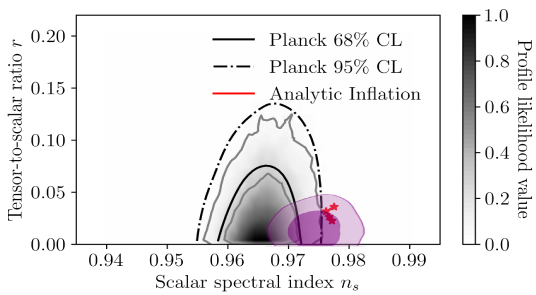
We can easily investigate the phenomenology of the model for the various values of the parameter $m$ which recall that it is constrained as in Eq. (11). Let us give some examples by choosing the $e$-foldings number in the range $N\sim 50-60$. So for example if $m=6$ and $N=55.5$ we get, $n_{\mathcal{S}}=0.977528$ and $r=0.0359549$ which are compatible with the ACT and the updated BICEP/Planck data. Generally, for compatibility with the ACT and the updated BICEP/Planck data we need $m\geq 6$. Note that the current model cannot yield a spectral index compatible with the Planck data, for any allowed value of the parameter $m$. So this model is suited perfectly only for the ACT-compatible inflationary theories. Other characteristic set of $(m,N)$ values compatible with the ACT and updated BICEP/Planck data are, $m=8$ and $N=50.5$ we get, $n_{\mathcal{S}}=0.976285$ and $r=0.0316204$, or for example $m=10$ and $N=50$ we get, $n_{\mathcal{S}}=0.976706$ and $r=0.0263591$, or for $m=14$ and $N=50$ we get, $n_{\mathcal{S}}=0.977176$ and $r=0.022598$. In Fig. 1 we confront the phenomenology of the model for various $N$ values in the range $N\sim 50-60$ and $m$ in the range $m=[6,14]$ and as it can be seen the model is compatible with the ACT and the updated Planck data. Now the question is, does the parameter $m$ affect the slow-roll conditions? For example if $m$ gets extremely large values, does it make the model incompatible with the slow-roll conditions? We can easily examine this by expanding the first slow-roll index (76) for very large $m$ values. In fact a particularly interesting behavior occurs in the observational indices in the large $m$ limit, and specifically, the spectral index in the large $N$ limit reads,

$$n_{\mathcal{S}}\simeq 1-\frac{1}{N}+\frac{1-2N}{mN^{2}}+\mathcal{O}\Big(\frac{1}{m^{3}}\Big)\,,$$ (81)

so it is basically independent of the parameter $m$ and behaves as $n_{\mathcal{S}}\simeq 1-\frac{1}{N}$. On the other hand the tensor-to-scalar ratio behaves as,

$$r\sim\frac{16}{mN}-\frac{16(2N+1)}{m^{2}N^{2}}+\mathcal{O}\Big(\frac{1}{m^{3}}\Big)\,.$$ (82)

Thus for $N\sim 50-60$ the spectral index takes values in the range $N\sim[0.98-0.98333]$ and the tensor-to-scalar ratio takes particularly small values, since it strongly depends on the parameter $m$. On the other hand, the spectral index does not depend on the parameter $m$ and thus its behavior is regulated by the $e$-foldings number. Notice that the model at hand at large $m$ yields a very small tensor-to-scalar ratio and a spectral index of the order $n_{\mathcal{S}}\sim 0.98$ way more blue in comparison to the Planck acceptable values. This result can be useful for future searches that may validate the ACT data, or even find values in tension with even the ACT or Planck data.

Figure 1: Marginalized curves of the Planck 2018 data and the analytic slow-roll model (10), confronted with the ACT data, the Planck 2018 data, and the updated Planck constraints on the tensor-to-scalar ratio for $N\sim 50-60$ and $m$ in the range $\alpha=[6,14]$.

Another interesting behavior of the one-parameter inflationary model we developed is the functional dependence of the spectral index as a function of the tensor-to-scalar ratio. This is easily obtained, since $\epsilon_{1}=\frac{m}{2}\epsilon_{2}$ and $r=16\epsilon_{1}$, so we get,

$$n_{\mathcal{S}}=1-\frac{r}{4}-\frac{m}{16}\,r\,.$$ (83)

This is an exact relation and it shows one thing, that the model produces a universal curve in the $n_{s}-r$ plane, which makes it extremely easy to comply with ACT/Planck/BICEP constraints.

Now let us consider several other phenomenological features of the analytic slow-roll model of inflation. Let us first consider the running of the spectral index, which is defined as,

$$a_{s}=\frac{\mathrm{d}n_{\mathcal{S}}}{\mathrm{d}\ln k}\,,$$ (84)

with $k$ being the comoving wavenumber corresponding to a primordial inflationary mode. We can write the running of the spectral index $a_{s}$ in the following form,

$$a_{s}=\frac{\mathrm{d}n_{\mathcal{S}}}{\mathrm{d}\ln k}=\frac{\mathrm{d}n_{\mathcal{S}}}{\mathrm{d}N}\frac{\mathrm{d}N}{\mathrm{d}\ln k}\,,$$ (85)

where $N$ is the $e$-foldings number. In addition, by using the formula $\frac{\mathrm{d}N}{\mathrm{d}\ln k}=\frac{1}{1-\epsilon_{1}}$, we can obtain the following simple formula for the running of the spectral index $a_{s}$,

$$a_{s}=\frac{1}{1-\epsilon_{1}}\frac{\mathrm{d}n_{\mathcal{S}}}{\mathrm{d}N}\,.$$ (86)

So for the model at hand, by using Eqs. (86), (76) and (77), we have,

$$a_{s}=\frac{m+4}{N\Big(1+(m+2)N\Big)}\,.$$ (87)

A striking first feature is that the running of the spectral index is positive, in contrast to well-known inflationary models, like for example the Starobinsky or the Higgs model. It is interesting to note that the ACT data point towards a positive running of the spectral index,

$$\frac{\mathrm{d}n_{\mathcal{S}}}{\mathrm{d}\ln k}=0.0062\pm 0.0052\,\,\,(68\%)\,,$$ (88)

but with a very small statistic significance $1.2\sigma$. Thus if this statistical preference of inflationary models with positive running of the spectral index becomes stronger in the future, the model at hand might be one of the few models in the context of general relativity that can produce a positive running. Let us compute some characteristic values, so for $(m,N)=(6,55.5)$ we get, $a_{s}=0.000404899$, while for $(m,N)=(8,50.5)$ we get, $a_{s}=0.000469612$. Also for $(m,N)=(10,50)$ we get, $a_{s}=0.00046589$ and for $(m,N)=(14,50)$ we get, $a_{s}=0.000449438$. All these values are well fitted within the ACT data, and we used the same $(m,N)$ pairs that we used to examine the compatibility of the spectral index and the tensor-to-scalar ratio with the ACT/BICEP/Planck data. Let us also find the asymptotic behavior of the running of the spectral index at large $m$ values, and it reads,

$$a_{s}\simeq\frac{1}{N^{2}}+\frac{1-4N^{2}}{m^{2}N^{4}}+\frac{2N-1}{mN^{3}}+\mathcal{O}\Big(\frac{1}{m^{3}}\Big)\,,$$ (89)

thus the large $m$ values do not affect the viability of the running of the spectral index, since for $N\sim 50-60$, the running of the spectral index is in the range $a_{s}^{asympt}\sim[0.0004,0.000277778]$, which are well fitted within the ACT constraints.

It is useful to find the values of the effective equation of state (EoS) parameter at the end of inflation (at $N=0$) and at the beginning of the inflationary era (at $N\sim 50-60$). We have,

$$w_{eff}=-1-\frac{2}{3}\frac{\dot{H}}{H^{2}}=-1+\frac{r}{24}\,,$$ (90)

with $r$ given in Eq. (80), and $w_{eff}$ must have the value $w_{eff}=-1/3$ at the end of inflation (at $N=0$) while it must be near $w_{eff}=-1$ at the beginning of inflation (at $N\sim 50-60$). Indeed, for $N=0$, the EoS parameter is $w_{eff}=-\frac{1}{3}$ and it is independent of the value of $m$ as it can easily be checked. Also the value of the EoS parameter at first horizon crossing, for $(m,N)=(6,55.5)$ is $w_{eff}=-0.998502$, while for $(m,N)=(8,50.5)$ we get, $w_{eff}=-0.998682$. Also for $(m,N)=(10,50)$ we get, $w_{eff}=-0.998891$ and for $(m,N)=(14,50)$ we get, $w_{eff}=-0.999168$. Thus, as $m$ increases, the EoS parameter approaches the quasi-de Sitter value $w_{eff}=-1$. This is particularly interesting and can easily be validated by taking the asymptotic form of Eq. (90) in the large $m$ regime, and we have,

$$w_{eff}^{asympt}\simeq-1+\frac{2}{3mN}-\frac{2(2N+1)}{3m^{2}N^{2}}\,.$$ (91)

This is reasonable, since the main assumption of this work materialized by Eq. (10), in the limit $m\to\infty$ yields a pure slow-roll evolution, with $w_{eff}\sim-1$ and a de-sitter regime with $\dot{\phi}\sim 0$. The behavior $w_{eff}\sim-1$ is allegedly attributed to a quasi-de Sitter evolution, however, we shall prove in a later section that the quasi-de Sitter evolution is obtained by the condition $\dot{\phi}^{2}=\kappa^{-4}\delta$, where $\delta$ is an arbitrary dimensionless parameter.

Now let us focus on the amplitude of the scalar perturbations, which we proved that in the case at hand, it is given by Eq. (72) evaluated at the first horizon crossing. So in view of Eq. (10), the amplitude of the scalar perturbations at first horizon crossing (when the CMB pivot scale exits the Hubble horizon during inflation at $N_{*}\sim 50-60$) takes the final form,

$$A_{s}=\frac{H_{*}^{m+4}}{4\pi^{2}\gamma}\,,$$ (92)

so when evaluated at the pivot scale, we get,

$$A_{s}=\frac{2^{-\frac{3m+8}{m+2}}\beta^{\frac{2}{m+2}}\Big((m+2)N_{*}+1\Big)^{\frac{m+4}{m+2}}\tau^{\frac{2m}{m+2}}}{\pi^{2}}\,,$$ (93)

where we introduced the notation,

$$H_{0}=\frac{\tau}{\kappa}\,,$$ (94)

with $\tau$ being a dimensionless parameter, and also we used the definition of $\gamma$ in Eq. (9). Also we shall use the fact that $\omega=\lambda\kappa^{-m-1}$. Now we can evaluate the constraints on the parameter $\beta$ and $\tau$ that may yield an inflationary theory compatible with the Planck data. Notice that the observational indices do not depend on $\tau$ and $\beta$. In addition, we may examine the behavior of the scale factor and of the Hubble rate as a function of the cosmic time. The resulting picture is particularly interesting. For simplicity let us choose only one $m$ for the presentation. The generalization is easy. In order to make the plots easier, due to the huge numbers appearing in the exponential of the scale factor, we shall rescale the cosmic time as follows:

$$t=\eta\kappa\,,$$ (95)

with $\eta$ being just an arbitrary dimensionless parameter, not to be confused with the conformal time. In terms of the $\eta$ parameter, the final cosmic time $\eta_{f}$ at which inflation ends is $\eta_{f}=\frac{t_{f}}{\kappa}$, and specifically,

$$\eta_{f}=\frac{2\lambda\tau^{-m}}{\beta}-\frac{2^{\frac{1}{m+2}}\,(m+2)\,\beta^{-\frac{1}{m+2}}}{(m+1)^{2}}\,,$$ (96)

and the time instance $\eta_{i}$ that inflation begins is,

$$\eta_{i}=\frac{\tau^{-m}\left(2\lambda(m+1)-2^{\frac{1}{m+2}}(m+2)^{\frac{m+1}{m+2}}\beta^{\frac{m+1}{m+2}}\tau^{\frac{m(m+1)}{m+2}}\left(\frac{\tau^{-m}\left(\left(m^{2}+3m+2\right)N\tau^{m}+(m+1)^{\frac{1}{m+1}}(m+2)^{\frac{m+2}{m+1}}\tau^{\frac{m(m+2)}{m+1}}\right)}{(m+1)(m+2)}\right)^{\frac{m+1}{m+2}}\right)}{\beta(m+1)}\,.$$ (97)

Setting $a_{0}=1$ in the scale factor (14), the scale factor in terms of $\eta$ reads,

$$a(\eta)=\exp\left(-\frac{2^{-\frac{1}{m+1}}(m+1)^{\frac{1}{m+1}+1}\tau^{-m}\left(2\lambda-\beta\eta\tau^{m}\right)^{\frac{m+2}{m+1}}}{\beta(m+2)}\right)\,,$$ (98)

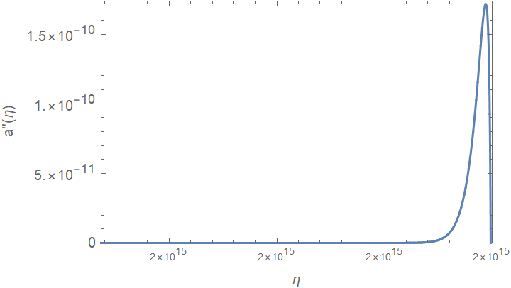
where we used the fact that $\omega=\lambda\kappa^{-m-1}$. The physical picture is clear, the Universe starts from an non-singular point, at $t=0$, and remarkably in the context of this model, there is no initial singularity. As the cosmic time grows, the slow-roll inflationary regime starts at $\eta=\eta_{i}$ ($t_{i}$) and ends at $\eta=\eta_{f}$ ($t_{f}$). The Universe reaches the critical time $\eta_{T}=\frac{2\lambda\tau^{-m}}{\beta}$, at which point the scale factor takes the maximum value, but the Hubble rate becomes equal to zero, since recall that the Hubble rate in terms of $\eta$ is expressed as follows,

$$H(\eta)=2^{-\frac{1}{m+1}}(m+1)^{\frac{1}{m+1}}\Big(2\lambda-\beta\eta\tau^{m}\Big)^{\frac{1}{m+1}}\,.$$ (99)

Now this is reminiscent of a bounce, but it is not. It is a turnaround cosmological evolution, with a pressure singularity at the critical point $\eta_{T}=\frac{2\lambda\tau^{-m}}{\beta}$, because the derivative of the Hubble rate diverges severely in that point. Thus, the energy density and the scale factor are finite for this cosmological evolution, but the derivative of the Hubble rate diverges. This is a typical pressure finite-time singularity according to the Nojiri-Odintsov-Tsujikawa classification Nojiri:2005sx . If the evolution remains classical, after the turnaround point, the scale factor decreases and the Universe collapses. However, we will show in a later section, that when the singularity is reached, quantum phenomena occur and the conformal anomaly due to conformal particles dominates the evolution, rendering the classical solution inactive, and at the same time, the Universe becomes radiation dominated due to severe particle production, thus offering a theory for reheating without scalar oscillations and numerous couplings of the inflaton to the Standard Model particles. Also thermal effects by the horizon of the finite-time singularity may also shift the classical evolution from being singular, since once the singularity is approached, these phenomena initiate and render the pre-turnaround point classical evolution inactive. These are very interesting physical phenomena and will be analyzed in depth in a later section. At this point, we shall be interested in the classical evolution without taking into account the quantum phenomena or the thermal phenomena near the singularity.

Figure 2: Graphical presentation of the scale factor $a(\eta)$ (upper left), the Hubble rate (upper right) as a function of the rescaled dimensionless time variable $\eta$, before the turnaround point. Also in the bottom left plot we present the Hubble radius $R_{H}(\eta)$ and in the bottom right the acceleration $a^{\prime\prime}(\eta)$ for the time interval for which inflation occurs $(\eta_{i},\eta_{f})$. We used the values of the free parameters that yield a viable inflationary evolution $(m,N)=(6,55.5)$ and $(\beta,\eta,\lambda)=(10^{-20},10^{-3},10^{-23})$.

So we shall prove that the evolution is indeed inflationary up to $\eta_{f}$ and also we will prove that the Hubble horizon shrinks during the inflationary regime, and also we shall show that the Hubble rate changes sign at the turnaround point, which indicates a turnaround cosmology. Recall that $m$ was assumed to be an even number, thus after the turnaround point, the Hubble rate is,

$$H(\eta)=-2^{-\frac{1}{m+1}}(m+1)^{\frac{1}{m+1}}\Big(-2\lambda+\beta\eta\tau^{m}\Big)^{\frac{1}{m+1}}\,.$$ (100)

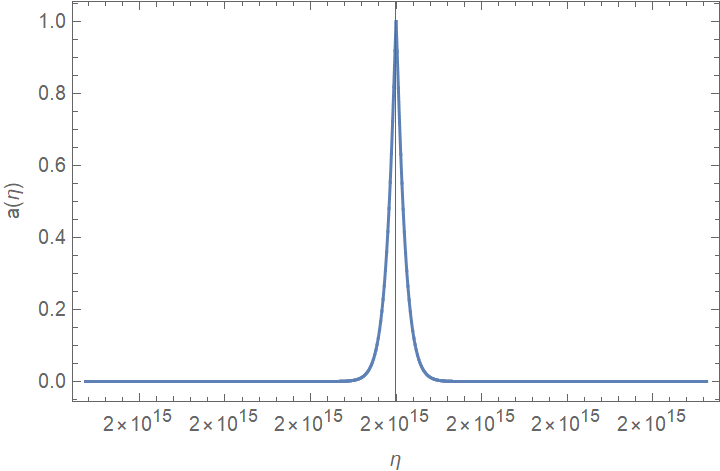
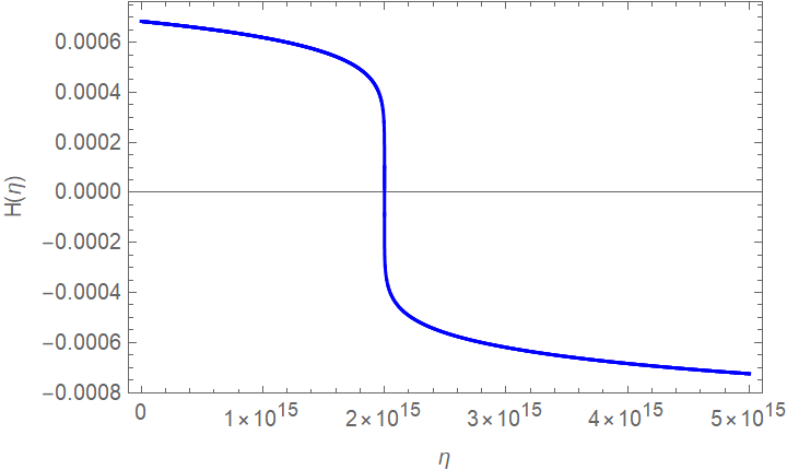
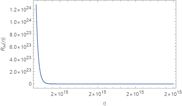
In order to make some graphical presentations of the evolution, let us find a viable set of parameters $\beta$, $\tau$ and $\lambda$ which make the amplitude of the scalar perturbations (93) compatible with the Planck constraint $A_{s}\sim 2.19\times 10^{-9}$ Planck:2018jri . We choose $(m,N)=(6,55.5)$ which yielded a viable inflationary phenomenology. A viable set of $(\beta,\eta,\lambda)$ values that makes the model to have an amplitude of scalar perturbations compatible with the Planck constraint is $(\beta,\eta,\lambda)=(10^{-20},10^{-3},10^{-23})$, and we chose $\lambda$ so small because physically, the inflationary era occurs at cosmic times of the order $t\sim\mathcal{O}(10^{-25})$sec. In Fig. 2 we plot the behavior of the scale factor before the turning point and after, the behavior of the Hubble rate before and after the turning point, the evolution of the Hubble radius $R_{H}=\frac{1}{H(\eta)a(\eta)}$ and the acceleration $a^{\prime\prime}(\eta)$ in the time interval $(\eta_{i},\eta_{f})$. As it can be verified from Fig. 2, the evolution is indeed inflationary in the time interval $\Delta\eta=(\eta_{i},\eta_{f})$. Also notice the plots that the values $\eta_{i}$ and $\eta_{f}$ are very close to the turnaround point $\eta_{T}$. If we add $\kappa$ in natural units, then the order of magnitude of $t_{i}$ would be $\mathcal{O}(10^{-25})$sec approximately. But this is just a graphical presentation, the physical picture is clear.

Now viewed as dynamical system, the analytic scalar field inflation model we developed is quite simple. The phase space is reduced to simple curves differing only in the initial conditions used each time. The $\dot{H}-H$ system closes under the equation,

$$\dot{H}=-\frac{\kappa^{2}}{2}\gamma H^{-m}.$$ (101)

This equation is autonomous in $H$ alone and it defines a one-dimensional invariant manifold, determined by,

$$\mathcal{M}:\qquad\dot{\phi}^{2}-\gamma H^{-m}=0.$$ (102)

The flow never leaves this surface once initial data lie on it, thus the system of the above equations, reduces the initial three-dimensional phase space $(\phi,\dot{\phi},H)$ of a minimally coupled scalar field theory, to an effectively one-dimensional flow. Let us analyze the trajectories in the $\phi-\dot{\phi}$ plane, for various values of $H_{0}$, $\beta$, $m$ and $\phi_{0}$. Note that in ordinary scalar field theory, the phase space analysis is impossible to do for general potentials, and it is done only for exponential potentials. Thus the general trajectories for general scalar field theories in the $H-\dot{H}$ and in the $\phi-\dot{\phi}$ planes cannot be found. In the case at hand, this is a trivial plot, since the trajectories are unique curves, differing only on the initial conditions, and the parameter values. To this end we will rescale the scalar field $\phi=\frac{\varphi}{\kappa}$ where $\varphi$ is a dimensionless variable.

Figure 3: The trajectories in the $\dot{\varphi}-\varphi$ space, for $\varphi=2$ (red curve) and $\varphi=4$ (blue curve), in the range $(\varphi_{i},\varphi_{f})$. We used the values of the free parameters that yield a viable inflationary evolution $(m,N)=(6,55.5)$ and $(\beta,\eta,\lambda)=(10^{-20},10^{-3},10^{-23})$.

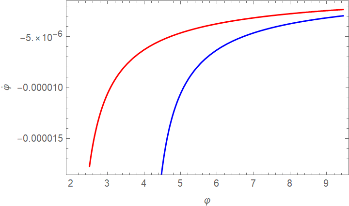
We can easily find by eliminating the cosmic time between $\phi$ and $\dot{\phi}$, that the derivative of the scalar field as a function of the scalar field is given as,

$$\dot{\varphi}=-\frac{4^{\frac{m}{m+2}}\,(m+2)^{-\frac{m}{m+2}}\beta^{\frac{1}{m+2}}\,\tau^{\frac{m}{m+2}}\,\Big(\varphi-\varphi_{0}\Big)^{-\frac{m}{m+2}}}{\kappa^{2}}\,.$$ (103)

For $m=6$ and for the values of the free parameters we used earlier, we can easily find the initial and final values of the scalar field, which are,

$$\phi_{i}=\frac{7.44988}{\kappa}+\phi_{0}\,,$$ (104)

$$\phi_{f}=\frac{0.0197297}{\kappa}+\phi_{0}\,,$$ (105)

where $\phi_{0}$ is the initial condition of the scalar field. In Fig. 3 we plot the trajectories in the $\dot{\varphi}-\varphi$ space, for $\varphi=2$ (red curve) and $\varphi=4$ (blue curve), in the range $(\varphi_{i},\varphi_{f})$. As it can seen, the trajectory is a single curve depending on the initial condition. Also notice that $\dot{\varphi}$ is singular at $\varphi=\varphi_{0}$.

II.4 Other Analytic Solutions and Their Inflationary Features

At this point, it is worth discussing other analytic solutions of Eq. (10) for various values of $m$. We shall consider the cases $m=0$ and $m=-2$ separately from the previous formalism. Let us consider first the equation,

$$\dot{\phi}^{2}=\gamma\,,$$ (106)

so from the Raychaudhuri equation we get,

$$2\dot{H}=-\kappa^{2}\gamma\,,$$ (107)

which yields an exact quasi-de Sitter evolution,

$$H(t)=H_{0}-\frac{1}{2}\gamma\kappa^{2}t\,,$$ (108)

and the scalar field as a function of the cosmic time is,

$$\phi(t)=\phi_{0}-\sqrt{\gamma}t\,.$$ (109)

The scalar field potential as a function of the scalar field is easily found,

$$V(\phi)=-\frac{\gamma}{2}+\frac{3\Big(\sqrt{\gamma}\kappa^{2}(\phi-\phi_{0})+2\phi_{0}\Big){}^{2}}{4\kappa^{2}}\,.$$ (110)

Accordingly, we can find $\epsilon_{1}$, and $\epsilon_{2}=0$ and the resulting observational indices are at leading order,

$$n_{\mathcal{S}}\simeq 1-\frac{2}{N}\,,$$ (111)

$$r=\frac{8}{N}-\frac{4}{N^{2}}\,.$$ (112)

The resulting phenomenology is non-viable however, since although the spectral index is accommodated easily in the Planck data, the tensor-to-scalar ratio is very large for $N\sim 50-60$.

Let us also consider the scenario $\dot{\phi}^{2}=\gamma H^{2}$, which is well known in the literature, since it yields an exponential scalar field potential and a power-law inflationary evolution, with eternal inflation. Indeed,

$$\dot{\phi}^{2}=\gamma H(t)^{2}\,,$$ (113)

so from the Raychaudhuri equation we get,

$$2\dot{H}=-\kappa^{2}\gamma H(t)^{2}\,,$$ (114)

which yields an exact power-law inflationary evolution,

$$H(t)=\frac{2}{\gamma\kappa^{2}t-2c_{1}}\,,$$ (115)

and the scalar field as a function of the cosmic time is,

$$\phi(t)=2c_{2}-\frac{2\log\left(\gamma\kappa^{2}t-2c_{1}\right)}{\sqrt{\gamma}\kappa^{2}}\,.$$ (116)

The scalar field potential as a function of the scalar field is easily found,

$$V(\phi)=-\frac{2\left(\gamma\kappa^{2}-6\right)e^{\sqrt{\gamma}\kappa^{2}(\varphi-2c_{2})}}{\kappa^{2}}\,.$$ (117)

This model leads to a constant EoS evolution, and it leads to an eternal inflation behavior, which cannot be viable with the Planck data. So we will not further discuss this case. See however, how such an exponential inflation scenario can be combined with other physical scenarios and solve the trans-Planckian issues of scalar field inflation Brandenberger:2004kx ; Martin:2003kp ; Martin:2000xs ; Odintsov:2026prn ; Odintsov:2025mqq .

III Inflation Ending at a Pressure Singularity, Quantum Phenomena, the Reheating, Gravitational Waves and Primordial Black Holes

Now let us focus on the interesting part of the singular analytic slow-roll scenario. What we have as a physical picture is a Universe starting from a non-singular point $t=0$ with finite scale factor, so a non-singular initial scale factor. Accordingly, the mini, non-singular Universe starts to expand exponentially, reaching an inflationary era which ends before a classical turning point $t=t_{c}$, where the Universe develops a pressure singularity. Classically, if the turning point is reached, a maximum size is reached, and beyond that, the Universe would start to contract exponentially. Now this is where the interesting physics enter, since once the pressure singularity is approached, the quantum effects would become dominant and the classical solution with $\dot{\phi}^{2}\sim H^{-m}$ would become inapplicable. Such an analysis was performed in Nojiri:2005sx , using both the conformal anomaly and the thermal effects of the singularity horizon. Here after we shall call this mechanism the Nojiri-Odintsov conformal anomaly effect, for simplicity.

Before quantifying the analysis it is worth recalling the classification of finite-time singularities, and show why the finite-time singularity of the analytic singular inflation is a pressure singularity. We will use the Nojiri-Odintsov-Tsujikawa classification of finite-time singularities Ref. Nojiri:2005sx , so the cosmic time singularities are classified as follows (see also the review deHaro:2023lbq ),

• Type I (“Big Rip”) Ref. Caldwell:2003vq ; Nojiri:2003vn ; Elizalde:2004mq ; Faraoni:2001tq ; Singh:2003vx ; Wu:2004ex ; Sami:2003xv ; Stefancic:2003rc ; Chimento:2003qy ; Zhang:2005eg ; Dabrowski:2006dd ; Nojiri:2009pf ; Capozziello:2009hc : Typical crushing type singularity with geodesics incompleteness. As the singularity point at $t\to t_{s}$ is reached, the scale factor $a(t)$, the effective pressure $p_{\mathrm{eff}}$ and the effective energy density $\rho_{\mathrm{eff}}$ diverge. The Universe cannot pass smoothly through this singularity. It is a crushing type spacelike singularity, at the spacelike hypersurface $t=t_{s}$ all the physical quantities that can be defined on it strongly diverge.

• Type II (“sudden” or “pressure singularity”): Milder than the Big Rip scenario, also known as a pressure singularity Barrow:2004xh ; Nojiri:2004ip ; Barrow:2004he ; FernandezJambrina:2004yy ; BouhmadiLopez:2006fu ; Barrow:2009df ; BouhmadiLopez:2009jk ; Barrow:2011ub ; Bouhmadi-Lopez:2013tua ; Bouhmadi-Lopez:2013nma ; Chimento:2015gum ; Cataldo:2017nck , see also Balcerzak:2012ae ; Marosek:2018huv . The Universe can pass smoothly through this singularity. It is not a crushing type spacelike singularity, and at the spacelike hypersurface $t=t_{s}$ the physical quantities that can be defined on it are smooth, that is the scale factor and the energy density, but only the effective pressure diverges at $t=t_{s}$, that is $a\to a_{s}$, $\rho_{\mathrm{eff}}\to\rho_{s}$ and $\left|p_{\mathrm{eff}}\right|\to\infty$.

• Type III : Stronger than the Type II, the effective pressure and the effective energy density diverge and the scale factor remains finite.

• Type IV : The smoothest of all the finite-time singularities Nojiri:2004pf ; Nojiri:2005sx ; Nojiri:2005sr ; Barrow:2015ora ; Nojiri:2015fra ; Nojiri:2015fia ; Odintsov:2015zza ; Oikonomou:2015qha . In this case, all the physical quantities remain finite on the spacelike hypersurface $t=t_{s}$. For this singularity, the graceful exit from the inflationary era may be occur due to this soft singularity Odintsov:2015gba .

Regarding the total pressure and total energy density $\rho_{\mathrm{eff}}$ and $p_{\mathrm{eff}}$, these are defined as,

$$\rho_{\mathrm{eff}}\equiv\frac{3}{\kappa^{2}}H^{2}\,,\quad p_{\mathrm{eff}}\equiv-\frac{1}{\kappa^{2}}\left(2\dot{H}+3H^{2}\right)\,,$$ (118)

which may receive contributions in our case from the scalar field and from matter fluids. During inflation the matter fluids generate a subdominant effect and thus do not affect the evolution $H(t)$, which is solely determined by the scalar field.

Now for the scenario of analytic singular inflation, the singularity at the turning point is a typical pressure singularity, since the scale factor acquires its maximum value and is finite, the Hubble rate is zero, and thus finite, but $\dot{H}$ diverges. Note that this reminds a bounce, but it is not, since in a bounce, we would have,

$$H<0\rightarrow H=0\rightarrow H>0$$

meaning that,

$$\begin{array}[]{c|c}\text{Phase}&\text{Evolution}\\ \hline\cr H<0&\text{contraction}\\ H=0&\text{bounce}\\ H>0&\text{expansion}\end{array}$$

In our case the sequence is,

$$H>0\rightarrow H=0\rightarrow H<0,$$

which is a cosmological turnaround behavior. Now it is important to note that in the context of the scenario we proposed for inflation, the EoS behaves as

$$w_{eff}=-1+\frac{1}{3}\gamma\kappa^{2}2^{n}(m+1)^{-n}\Big(-\gamma\kappa^{2}t+2\omega\Big){}^{-n}\,,$$ (119)

thus it has a singularity at $t_{*}=\frac{2\omega}{\gamma\kappa^{2}}$. So the model exhibits a sort of sudden singularity at the turnaround point $t_{*}=\frac{2\omega}{\gamma\kappa^{2}}$, which either means that the scalar field theory is ineffective beyond the turnaround point, or simply the Universe exhibits a sudden singularity at that point. But apart from that, if we look at the potential at the Appendix, it is obvious that the potential also exhibits a singularity at $t=t_{*}$, so apparently, the theory has a pole at the turnaround point. This can also be seen by looking at Eq. (24) where the scalar field potential is expressed as a function of the scalar field, but it is less transparent compared to the $V(t)$ expression appearing at the Appendix.

Now here is the important part from a physical point of view. Matter fields are present during the singular analytic inflationary regime, but are disregarded as they cause subdominant effects and do not alter the Hubble rate. So classically, the Universe would reach the turnaround point and would go smoothly through the pressure singularity. However, once the pressure singularity is approached, the curvature invariants that contain $\dot{H}$ strongly diverge. Thus the quantum effects should be taken into account, or even thermal effects as in Ref. Nojiri:2020sti . Taking into account the thermal effects would eliminate the classical singular behavior and this is a well known feature in the literature Nojiri:2004ip ; Nojiri:2004pf ; Kamenshchik:2013naa ; Bates:2010nv ; Tretyakov:2005en ; Calderon:2004bi ; Carlson:2016iuw ; Nojiri:2010wj . Thus the classical trajectory $\dot{\phi}^{2}\sim H^{-m}$ would not longer determine the evolution of the Universe. In this work we shall use the Nojiri-Odintsov conformal anomaly effects Nojiri:2020sti and discuss how these smooth out the pressure singularity and more importantly they generate a natural reheating mechanism for the Universe without requiring field oscillations and numerous couplings of the inflaton to the Standard Model particles.

The mechanism is simple, when quantum matter fields are included, the gravitational dynamics is described by the semiclassical Einstein equations,

$$G_{\mu\nu}=8\pi G\left(T_{\mu\nu}^{\mathrm{class}}+\langle T_{\mu\nu}^{\mathrm{quantum}}\rangle\right).$$ (120)

The quantum expectation value of the stress tensor can be decomposed schematically as follows,

$$\langle T_{\mu\nu}^{\mathrm{quantum}}\rangle=T_{\mu\nu}^{\mathrm{vac}}+T_{\mu\nu}^{\mathrm{anom}}+T_{\mu\nu}^{\mathrm{state}},$$ (121)

with the contributions corresponding to, vacuum polarization, the conformal anomaly, and state-dependent particle production. In many cosmological applications only the anomaly term is retained because it is universal and independent of the quantum state and this is what we adopt here too. Classically, conformally invariant fields, that is, classically massless fields, satisfy,

$$T^{\mu}_{\ \mu}=0.$$ (122)

Quantum mechanically this relation is violated due to renormalization effects, yielding the so-called trace anomaly,

$$\langle{T^{\mu}_{\mu}}_{A}\rangle=bF+b^{\prime}\mathcal{G}+b^{\prime\prime}\Box R,$$ (123)

with, $F$ being the square of the Weyl tensor, $\mathcal{G}$ being the Gauss-Bonnet invariant, and $R$ being the Ricci scalar. Examples of conformal fields that contribute to the conformal anomaly include, photons, gluons, massless fermions, and perhaps extra conformally coupled scalar fields (string theory remnants). Let us further elaborate on the calculation of the conformal anomaly for the case at hand, and how the Nojiri-Odintsov conformal anomaly smooths the pressure singularity in the original scenario we had. The conformal anomaly $T_{A}$ is,

$$T_{A}=b\left(\mathcal{F}+\frac{2}{3}\Box R\right)+b^{\prime}\mathcal{G}+b^{\prime\prime}\Box R\,,$$ (124)

with $\mathcal{F}$ being the square of the 4D Weyl tensor, and also $\mathcal{G}$ is the Gauss-Bonnet invariant, which are given by

$$\mathcal{F}=\frac{1}{3}R^{2}-2R_{\mu\nu}R^{\mu\nu}+R_{\mu\nu\rho\sigma}R^{\mu\nu\rho\sigma}\,,\quad\mathcal{G}=R^{2}-4R_{\mu\nu}R^{\mu\nu}+R_{\mu\nu\rho\sigma}R^{\mu\nu\rho\sigma}\,.$$ (125)

Let the conformal matter fluids consist of $N$ scalars, $N_{1/2}$ spinors, $N_{1}$ vector fields, $N_{2}$ ($=0$ or $1$) gravitons, and also $N_{\mathrm{HD}}$ higher-derivative conformal scalars. Then the factors $b$ and $b^{\prime}$ are equal to,

$$b=\frac{N+6N_{1/2}+12N_{1}+611N_{2}-8N_{\mathrm{HD}}}{120(4\pi)^{2}}\,,\quad b^{\prime}=-\frac{N+11N_{1/2}+62N_{1}+1411N_{2}-28N_{\mathrm{HD}}}{360(4\pi)^{2}}\ ,$$ (126)

and thus $b$ is positive and $b^{\prime}$ is negative for the usual perfect fluid conformal matter fields. Now schematically, away from the singularity we have,

$$T_{A}\sim\frac{R^{2}}{(4\pi)^{2}},$$ (127)

but near the singularity we have,

$$T_{A}\sim H^{(3)},\quad H\ddot{H},\quad\dot{H}^{2}\,,$$ (128)

hence, if,

$$H^{(3)}\gg H^{2},$$ (129)

the anomaly contribution can dominate the dynamics of the Universe, even if classical matter densities are negligible. The semiclassical trace equation has the following form,

$$-R=8\pi G(T_{\phi}+T_{A})\,,$$ (130)

and near a Type II singularity one typically finds

$$T_{A}\gg R,$$ (131)

since,

$$\Box R\sim(t_{s}-t)^{-\beta-2}\,,$$ (132)

which diverges faster than

$$R\sim(t_{s}-t)^{-\beta}\,,$$ (133)

where we defined $\beta$ to be,

$$\beta=-\frac{1}{m+1}$$ (134)

from Eq. (13). Consequently the classical singular solution cannot satisfy the semiclassical equations, once the anomaly effect becomes dominant. Thus the quantum backreaction modifies the evolution and may remove the singularity. This is basically the Nojiri-Odintsov conformal anomaly mechanism. Let us quantify this mechanism even further, so,

$$R=-\frac{\kappa^{2}}{2}\left(T_{\mathrm{matter}}+T_{A}\right)\,.$$ (135)

For a FRW Universe, $\mathcal{F}$ and $\mathcal{G}$ are,

$$\mathcal{F}=0\ ,\quad\mathcal{G}=24\left(\dot{H}H^{2}+H^{4}\right)\ .$$ (136)

We assumed that $H$ behaves in the following way,

$$H\sim\left(t_{s}-t\right)^{-\beta}\,,$$ (137)

and recall $\beta=-\frac{1}{m+1}$ from Eq. (134). Since, $0>\beta>-1$ the singularity is a Type II or pressure singularity. In this case, we find that $\mathcal{G}\sim 24\dot{H}H^{2}\sim\left(t_{s}-t\right)^{-3\beta-1}$. Since $R\sim\left(t_{s}-t\right)^{-\beta-1}$, the Gauss-Bonnet term in $T_{A}$ is less singular compared with $R$. However, as we mentioned earlier, $\Box R$ behaves as $\Box R\sim\left(t_{s}-t\right)^{-\beta-3}$, thus it is more singular than the scalar curvature. Hence if $2b/3+b^{\prime\prime}\neq 0$, the contribution from $T_{A}$ in the trace equation (135) is more singular that $R$ near the pressure singularity. This simple dominant balance analysis, simply shows that the solution (13) no longer satisfies the trace equation (135), thus the Type II singularity is avoided due to the quantum effects near the pressure singularity.

Now this pressure singularity actually offers an elegant reheating mechanism, without resorting to scalar field oscillations and having the awkward necessity of coupling the inflaton differently to all the Standard Model particles. The line of thinking is the following, quantum particle production occurs when the background spacetime evolves rapidly. In an expanding Universe, the production rate of particles roughly scales with the effective frequency variation of modes, which is governed by the scale factor. Dimensionally one finds,

$$\Gamma\sim\left|\frac{a^{\prime\prime}}{a}\right|,$$ (138)

where primes denote derivatives with respect to conformal time. Equivalently, in terms of the cosmic time, this corresponds approximately to,

$$\Gamma\sim|\dot{H}|+H^{2}.$$ (139)

Near a sudden (Type II) singularity the second derivative of the scale factor diverges,

$$\ddot{a}\rightarrow\infty,$$ (140)

which implies,

$$\frac{a^{\prime\prime}}{a}\rightarrow\infty.$$ (141)

Consequently, the vacuum modes are excited violently and particle production becomes extremely efficient. The produced particles generate radiation and can significantly affect the cosmic evolution. The resulting cosmological scenario can be summarized as the following sequence, no-singular emergence of the Universe, followed by a slow-roll inflationary regime, after which the Universe approaches a sudden Singularity, then quantum effects smooth out the singularity, causing severe particle production, which generates a radiation domination era. The Universe after that evolves classically. The energy density of produced particles can be estimated as,

$$\rho_{r}\sim\int|\beta_{k}|^{2}\,k\,d^{3}k,$$ (142)

where $\beta_{k}$ are Bogoliubov coefficients describing particle production. When derivatives of the curvature become large, $|\beta_{k}|^{2}$ increases significantly and the radiation energy density grows rapidly, producing backreaction on the expansion, thus we have,

$$\rho_{r}\sim T^{4},$$ (143)

which effectively reheats the Universe.

However, there are more important consequences in the Universe due to the pressure singularity. Specifically, near the pressure singularity, the scalar perturbations would be enhanced and thus primordial black holes may be formed and in addition secondary gravitational waves may be generated with observable features in the energy spectrum from future gravitational wave experiments. Let us qualitatively analyze these in brief. Specifically, the scalar perturbations obey the Mukhanov-Sasaki equation,

$$v_{k}^{\prime\prime}+\left(k^{2}-\frac{z^{\prime\prime}}{z}\right)v_{k}=0,$$ (144)

and in our case,

$$z=a\frac{\dot{\phi}}{H}.$$ (145)

Near a Type II singularity derivatives of the Hubble parameter diverge, which implies

$$\frac{z^{\prime\prime}}{z}\sim(t_{s}-t)^{-2}.$$ (146)

This produces a sharp spike in the power spectrum of the perturbations, leading to strong amplification of modes and possibly enhanced particle production. If the amplification of curvature perturbations becomes sufficiently large,

$$P_{\zeta}(k)\sim 10^{-2},$$ (147)

the resulting density fluctuations can collapse upon horizon re-entry and form primordial black holes. Apparently we are considering very small wavelength modes, immediately entering the horizon after the inflationary regime, and before the singularity is reached, so from $t=t_{f}$ to $t=t_{c}$. Thus a sudden singularity after the end of inflation may generate primordial black holes, on very small scales without affecting CMB observables. Such features typically occur on scales much smaller than those probed by the CMB. Therefore the relevant observational probes include primordial black holes, induced gravitational waves. Regarding the secondary gravitational waves, there are fundamental works appearing in the literature Sasaki:2025zao ; Sasaki:2025vql ; Gorji:2023ziy ; Ota:2022hvh ; Domenech:2021wkk ; Zhou:2020kkf ; Domenech:2020kqm ; Pi:2020otn ; Kuroyanagi:2017kfx ; Wu:2021zta ; Gao:2021vxb ; Gao:2020tsa ; Ragavendra:2020sop ; Lin:2020goi ; Lu:2019sti , and the logic in our context is the following, the evolution equation for tensor modes $h_{ij}$ is,

$$h_{ij}^{\prime\prime}+2\mathcal{H}h_{ij}^{\prime}-\nabla^{2}h_{ij}=4\mathcal{T}_{ij}^{\ \ lm}S_{lm},$$ (148)

where $\mathcal{H}=a^{\prime}/a$ is the conformal Hubble parameter and $\mathcal{T}_{ij}^{\ \ lm}$ is the transverse-traceless projection operator and the source term $S_{lm}$ is quadratic in scalar perturbations. Consequently, the enhanced scalar modes generated near the sudden singularity would produce a stochastic background of secondary gravitational waves. The corresponding energy density spectrum would be approximately,

$$\Omega_{\rm GW}(k)\sim\mathcal{O}(1)\,P_{\zeta}^{2}(k).$$ (149)

Therefore a burst of scalar amplification associated with a sudden singularity could potentially lead to a peaked spectrum of primordial gravitational waves on very small scales. Such signals may be connected to primordial black hole formation and could be probed by future high-frequency gravitational wave detectors.

III.1 Inflationary Effective Field Theory Scenarios and Beyond the UV-cutoff Physics

Another interesting interpretation near the pressure singularity is the effective field theory of inflation Cheung:2007st ; Weinberg:2008hq ; Senatore:2010wk ; Kallosh:2013hoa ; Galante:2014ifa . Specifically, we can imagine that the singular analytic scalar field inflation scenario is a part of an effective theory of inflation, which provides a framework for describing the dynamics of the inflationary phase, without specifying the detailed microphysical origin of the inflaton sector. The main idea is that, at energies well below a physically imposed cutoff scale $\Lambda$, the relevant degrees of freedom can be captured by an effective action organized as an expansion in operators consistent with the symmetries of the cosmological background. In single-field inflation, the time evolution of the background scalar field $\phi(t)$ spontaneously breaks time diffeomorphism invariance, thus leaving spatial diffeomorphisms unbroken. This allows the construction of the most general action governing the fluctuations around the quasi-de Sitter background. At the background level the dynamics is usually described by a canonical scalar field minimally coupled to gravity,

$$S=\int d^{4}x\sqrt{-g}\left[\frac{M_{\rm Pl}^{2}}{2}R-\frac{1}{2}(\partial\phi)^{2}-V(\phi)\right],$$

leading to the Friedmann equations.

$$3M_{\rm Pl}^{2}H^{2}=\frac{1}{2}\dot{\phi}^{2}+V(\phi),\qquad\dot{H}=-\frac{\dot{\phi}^{2}}{2M_{\rm Pl}^{2}},$$

and inflation occurs when the slow-roll parameters,

$$\epsilon=-\frac{\dot{H}}{H^{2}},\qquad\eta=\frac{\dot{\epsilon}}{H\epsilon}$$

remain small, $\epsilon\ll 1$ and $|\eta|\ll 1$, so that the expansion is approximately quasi-de Sitter. Within the effective field theory approach one constructs the most general action for perturbations around the inflationary background by fixing a unitary gauge, in which the scalar fluctuations are absorbed into the metric. The resulting action can be written schematically as,

$$S=\int d^{4}x\sqrt{-g}\left[\frac{M_{\rm Pl}^{2}}{2}R-M_{\rm Pl}^{2}\dot{H}g^{00}-M_{\rm Pl}^{2}(3H^{2}+\dot{H})+\sum_{n\geq 2}\frac{M_{n}^{4}}{n!}(\delta g^{00})^{n}+\cdots\right],$$

with the higher-order operators encoding the effects of unknown high-energy physics well above the cutoff scale. This formalism makes explicit that inflation should be regarded as an effective description, which is valid only within a specific evolutionary regime. The effective field theory perspective is particularly useful in our case, in which the scalar field derivative develops a pressure singularity after the inflationary era. In our case, after inflation and near the pressure singularity, the kinetic energy grows rapidly as the cosmic time approaches the turnaround point, thus driving the system toward the boundary of validity of the effective theory. This for example occurs when,

$$\dot{\phi}^{2}\sim\Lambda^{4},$$

and thus the higher-order operators in the effective action,

$$\mathcal{L}=\frac{1}{2}(\partial\phi)^{2}+\frac{1}{\Lambda^{4}}(\partial\phi)^{4}+\frac{1}{\Lambda^{8}}(\partial\phi)^{6}+\cdots,$$

which were disregarded, become dynamically more important and the canonical scalar description breaks down. From this viewpoint, singular behavior in the classical background evolution can be interpreted not as a fundamental physical singularity, but as an indication that the additional operators or extra effective field theory degrees of freedom must be taken into account for the dynamics. Hence, the effective field theory of inflation provides a robust framework for analyzing inflationary models, while at the same time being model agnostic about the UV completion of the theory. It may also justify how non-crushing type singularities may signal the breakdown of the low-energy classical scalar field description, and thus point out that the singularity is not a pathology of the fundamental theory, but an indication that the classical description breaks down once the kinetic energy of the scalar field becomes comparable in magnitude with the cut-off.

III.2 Inflationary Phase Transitions near the Pressure Singularity?

An interesting interpretation of the pole in $\dot{H}$ and the kinetic energy of the scalar field $\dot{\phi}^{2}$ appearing at the turnaround point $t=t_{c}$, is that it may actual indicate that a phase transition in the scalar sector takes place, rather than a true physical singularity. In this view the relation

$$\dot{\phi}^{2}=\gamma H^{-m}$$

is valid only for a particular effective phase of the total scalar field theory. As the cosmological evolution drives the system toward

$$H\rightarrow 0,$$

the kinetic energy grows rapidly,

$$\dot{\phi}^{2}\rightarrow\infty,$$

a fact that indicates, that the system approaches the boundary of validity of that phase. In many effective field theories, a divergence of this sort indicates that the theory is approaching a critical point, where new degrees of freedom become relevant. The scalar sector may undergo a transition in which the effective potential, the kinetic structure, or the vacuum state of the field changes. Quantitatively this can be simply realized by a scalar potential of the form,

$$V(\phi,\chi)=V_{1}(\phi)+g(\chi)\phi^{2},$$

with the auxiliary field or background quantity $\chi$ evolving with cosmic time. Such a formulation is also used in standard power-law inflationary scenarios to end the eternal inflation phase Odintsov:2026prn ; Odintsov:2025mqq . As the Universe expands ,and the Hubble parameter decreases, the effective mass of the scalar field,

$$m_{\rm eff}^{2}(\chi)=\frac{\partial^{2}V}{\partial\phi^{2}},$$

may change sign, so when,

$$m_{\rm eff}^{2}=0$$

the system reaches a critical point and the vacuum configuration of the scalar field changes. Such a phase transition can occur when the cosmological evolution reaches a specific value of the Hubble parameter. In this theoretical framework, the divergence of $\dot{\phi}^{2}$ near the point where $H=0$, could indicate that the field is being driven rapidly toward the new vacuum configuration. Instead of reaching an actual singularity, the scalar sector undergoes a dynamical transition that drastically modifies the effective theory. The original evolution,

$$\dot{\phi}^{2}=\gamma H^{-m}$$

is then replaced by a different dynamical evolution governed by the new phase. But this scenario is just another perspective, and one must rely on oscillations of the scalar fields in the new phase to explain reheating. Thus one must couple again the scalar field(s) with the Standard Model particles to explain the reheating and generate the radiation domination era. We believe that the Nojiri-Odintsov conformal anomaly approach for the reheating of the Universe in our context, is much more appealing theoretically. We aimed though to show the inflationary phase transitions perspective, also appearing in the literature in various forms Zou:2026wzi ; Bao:2026bgu ; Hu:2025xdt ; An:2023jxf ; An:2022toi ; Kamada:2011bt ; Abolhasani:2010kn ; Itzhaki:2008hs ; Dimopoulos:2022mce ; Gong:2022tfu ; Dimopoulos:2017qqn ; Kawasaki:2015ppx ; Lyth:2012yp ; Fonseca:2010nk

IV Conclusions

In this work we presented a class of minimally coupled scalar field models, which can realize a slow-roll era and can be solved fully analytically. We examined the solutions of the model, and we found that the models are essentially one parameter models and can be compatible with the ACT data. In fact in limiting cases, the models predict a bluer tilt of the spectral index near the value 0.98 and the tensor-to-scalar ratio tends to very small, nearly zero values. The cosmological solution describes a Universe which starts from a non-singular state and expands, realizing a slow-roll era. After the inflationary era ends, the cosmological system develops a pressure singularity at least classically, and the Universe reaches a maximum size and starts to contract. However, if we take into account the quantum phenomena near the singularity, the classical singularity is avoided, and more importantly these quantum anomalies induce a reheating mechanism which avoids oscillating scalar fields and its numerous couplings to the Standard Model particles. Thus the models we presented have the attribute of being able to study analytically, describe an initially non-singular emergent Universe, distinct from other emergent Universe scenarios Mulryne:2005ef ; Ellis:2002we ; Ellis:2003qz , the model produces a slow-roll inflationary era and develops a pressure singularity classically. The quantum phenomena near the singularity make the Universe avoid the singularity, and at the same time they provide a natural reheating mechanism after the inflationary era. In addition, the power spectrum might be enhanced, and thus the generation of primordial gravitational waves and of secondary gravitational waves is also a possibility.

Future perspectives of this work is including thermal horizon effects near the sudden singularity and extending the theoretical framework to k-inflationary theories, $F(R,\phi)$ gravity or even Einstein-Gauss-Bonnet gravity. We hope to address some of these tasks soon.

Appendix: Definition of Constants and of Lengthy Expressions

In this appendix we quote the scalar field potential as a function of the cosmic time. This can be found by using the Friedmann equation (6), and the solutions for the scalar field $\phi(t)$ given in Eq. (18) and the Hubble rate (13), so the scalar potential reads,

$$V(t)=4^{-\frac{1}{m+1}}\left(\frac{3(m+1)^{\frac{2}{m+1}}\Big(2\omega-\gamma\kappa^{2}t\Big)^{\frac{2}{m+1}}}{\kappa^{2}}-\gamma 2^{\frac{1}{m+1}}(m+1)^{-\frac{m}{m+1}}\Big(2\omega-\gamma\kappa^{2}t\Big)^{-\frac{m}{m+1}}\right)\,.$$ (150)

Also here we shall define the constants appearing in Eq. (24) which are,

$$\mathcal{K}=2^{\frac{3m^{2}+10m+6}{2(m+1)^{2}}}$$ (151)

and

$$\mathcal{B}=2^{\frac{-5m-4}{(m+1)^{2}}}(m+2)^{-\frac{2m}{m+2}}\gamma^{\frac{2}{m+2}}\kappa^{-\frac{4m}{m+2}}\,.$$ (152)

Finally, the parameter $\Gamma$ appearing in Eq. (75) is defined as follows,

$$\Gamma=-\frac{2^{-\frac{1}{m+1}}(m+1)^{n}\Big(2\omega-\gamma\kappa^{2}t_{f}\Big)^{n}}{\gamma\kappa^{2}(m+2)}\,.$$ (153)

References

- (1) A. D. Linde, Lect. Notes Phys. 738 (2008) 1 [arXiv:0705.0164 [hep-th]].
- (2) D. S. Gorbunov and V. A. Rubakov, “Introduction to the theory of the early universe: Cosmological perturbations and inflationary theory,” Hackensack, USA: World Scientific (2011) 489 p;
- (3) A. Linde, arXiv:1402.0526 [hep-th];
- (4) D. H. Lyth and A. Riotto, Phys. Rept. 314 (1999) 1 [hep-ph/9807278].
- (5) M. H. Abitbol et al. [Simons Observatory], Bull. Am. Astron. Soc. 51 (2019), 147 [arXiv:1907.08284 [astro-ph.IM]].
- (6) E. Allys et al. [LiteBIRD], PTEP 2023 (2023) no.4, 042F01 doi:10.1093/ptep/ptac150 [arXiv:2202.02773 [astro-ph.IM]].
- (7) S. Hild, M. Abernathy, F. Acernese, P. Amaro-Seoane, N. Andersson, K. Arun, F. Barone, B. Barr, M. Barsuglia and M. Beker, et al. Class. Quant. Grav. 28 (2011), 094013 doi:10.1088/0264-9381/28/9/094013 [arXiv:1012.0908 [gr-qc]].
- (8) J. Baker, J. Bellovary, P. L. Bender, E. Berti, R. Caldwell, J. Camp, J. W. Conklin, N. Cornish, C. Cutler and R. DeRosa, et al. [arXiv:1907.06482 [astro-ph.IM]].
- (9) T. L. Smith and R. Caldwell, Phys. Rev. D 100 (2019) no.10, 104055 doi:10.1103/PhysRevD.100.104055 [arXiv:1908.00546 [astro-ph.CO]].
- (10) J. Crowder and N. J. Cornish, Phys. Rev. D 72 (2005), 083005 doi:10.1103/PhysRevD.72.083005 [arXiv:gr-qc/0506015 [gr-qc]].
- (11) T. L. Smith and R. Caldwell, Phys. Rev. D 95 (2017) no.4, 044036 doi:10.1103/PhysRevD.95.044036 [arXiv:1609.05901 [gr-qc]].
- (12) N. Seto, S. Kawamura and T. Nakamura, Phys. Rev. Lett. 87 (2001), 221103 doi:10.1103/PhysRevLett.87.221103 [arXiv:astro-ph/0108011 [astro-ph]].
- (13) S. Kawamura, M. Ando, N. Seto, S. Sato, M. Musha, I. Kawano, J. Yokoyama, T. Tanaka, K. Ioka and T. Akutsu, et al. [arXiv:2006.13545 [gr-qc]].
- (14) A. Weltman, P. Bull, S. Camera, K. Kelley, H. Padmanabhan, J. Pritchard, A. Raccanelli, S. Riemer-Sørensen, L. Shao and S. Andrianomena, et al. Publ. Astron. Soc. Austral. 37 (2020), e002 doi:10.1017/pasa.2019.42 [arXiv:1810.02680 [astro-ph.CO]].
- (15) P. Auclair et al. [LISA Cosmology Working Group], [arXiv:2204.05434 [astro-ph.CO]].
- (16) G. Agazie et al. [NANOGrav], Astrophys. J. Lett. 951 (2023) no.1, L8 doi:10.3847/2041-8213/acdac6 [arXiv:2306.16213 [astro-ph.HE]].
- (17) S. Vagnozzi, JHEAp 39 (2023), 81-98 doi:10.1016/j.jheap.2023.07.001 [arXiv:2306.16912 [astro-ph.CO]].
- (18) V. K. Oikonomou, Phys. Rev. D 108 (2023) no.4, 043516 doi:10.1103/PhysRevD.108.043516 [arXiv:2306.17351 [astro-ph.CO]].
- (19) Y. Akrami et al. [Planck], Astron. Astrophys. 641 (2020), A10 doi:10.1051/0004-6361/201833887 [arXiv:1807.06211 [astro-ph.CO]].
- (20) T. Louis et al. [ACT], [arXiv:2503.14452 [astro-ph.CO]].
- (21) E. Calabrese et al. [ACT], [arXiv:2503.14454 [astro-ph.CO]].
- (22) P. A. R. Ade et al. [BICEP and Keck], Phys. Rev. Lett. 127 (2021) no.15, 151301 doi:10.1103/PhysRevLett.127.151301 [arXiv:2110.00483 [astro-ph.CO]].
- (23) R. Kallosh, A. Linde and D. Roest, [arXiv:2503.21030 [hep-th]].
- (24) Q. Gao, Y. Gong, Z. Yi and F. Zhang, [arXiv:2504.15218 [astro-ph.CO]].
- (25) L. Liu, Z. Yi and Y. Gong, [arXiv:2505.02407 [astro-ph.CO]].
- (26) Yogesh, A. Mohammadi, Q. Wu and T. Zhu, [arXiv:2505.05363 [astro-ph.CO]].
- (27) Z. Yi, X. Wang, Q. Gao and Y. Gong, [arXiv:2505.10268 [astro-ph.CO]].
- (28) Z. Z. Peng, Z. C. Chen and L. Liu, [arXiv:2505.12816 [astro-ph.CO]].
- (29) W. Yin, [arXiv:2505.03004 [hep-ph]].
- (30) C. T. Byrnes, M. Cortês and A. R. Liddle, [arXiv:2505.09682 [astro-ph.CO]].
- (31) W. J. Wolf, [arXiv:2506.12436 [astro-ph.CO]].
- (32) S. Aoki, H. Otsuka and R. Yanagita, [arXiv:2504.01622 [hep-ph]].
- (33) Q. Gao, Y. Qian, Y. Gong and Z. Yi, [arXiv:2506.18456 [gr-qc]].
- (34) M. Zahoor, S. Khan and I. A. Bhat, [arXiv:2507.18684 [astro-ph.CO]].
- (35) E. G. M. Ferreira, E. McDonough, L. Balkenhol, R. Kallosh, L. Knox and A. Linde, [arXiv:2507.12459 [astro-ph.CO]].
- (36) A. Mohammadi, Yogesh and A. Wang, [arXiv:2507.06544 [astro-ph.CO]].
- (37) S. Choudhury, G. Bauyrzhan, S. K. Singh and K. Yerzhanov, [arXiv:2506.15407 [astro-ph.CO]].
- (38) S. D. Odintsov and V. K. Oikonomou, Phys. Lett. B 868 (2025), 139779 doi:10.1016/j.physletb.2025.139779 [arXiv:2506.08193 [gr-qc]].
- (39) R. D. A. Q., J. Chagoya and A. A. Roque, [arXiv:2508.13273 [gr-qc]].
- (40) Y. Zhu, Q. Gao, Y. Gong and Z. Yi, [arXiv:2508.09707 [astro-ph.CO]].
- (41) G. Kouniatalis and E. N. Saridakis, [arXiv:2507.17721 [astro-ph.CO]].
- (42) M. Hai, A. R. Kamal, N. F. Shamma and M. S. J. Shuvo, [arXiv:2506.08083 [hep-th]].
- (43) C. Dioguardi, A. J. Iovino and A. Racioppi, Phys. Lett. B 868 (2025), 139664 doi:10.1016/j.physletb.2025.139664 [arXiv:2504.02809 [gr-qc]].
- (44) J. Yuennan, P. Koad, F. Atamurotov and P. Channuie, [arXiv:2508.17263 [astro-ph.CO]].
- (45) H. J. Kuralkar, S. Panda and A. Vidyarthi, [arXiv:2504.15061 [gr-qc]].
- (46) H. J. Kuralkar, S. Panda and A. Vidyarthi, JCAP 05 (2025), 073 doi:10.1088/1475-7516/2025/05/073 [arXiv:2502.03573 [astro-ph.CO]].
- (47) T. Modak, [arXiv:2509.02979 [astro-ph.CO]].
- (48) V. K. Oikonomou, [arXiv:2508.19196 [gr-qc]].
- (49) S. D. Odintsov and V. K. Oikonomou, [arXiv:2508.17358 [gr-qc]].
- (50) S. Aoki, H. Otsuka and R. Yanagita, [arXiv:2509.06739 [hep-ph]].
- (51) Z. Ahghari and M. Farhoudi, [arXiv:2512.12286 [gr-qc]].
- (52) E. McDonough and E. G. M. Ferreira, [arXiv:2512.05108 [astro-ph.CO]].
- (53) D. Chakraborty, M. Hai, S. T. Jahan, A. R. Kamal and M. S. J. Shuvo, [arXiv:2511.19610 [hep-th]].
- (54) S. Noori Gashti, M. A. S. Afshar, M. R. Alipour, B. Pourhassan and J. Sadeghi, Eur. Phys. J. C 85 (2025) no.11, 1343 doi:10.1140/epjc/s10052-025-15066-0
- (55) J. Yuennan, F. Atamurotov and P. Channuie, [arXiv:2511.17216 [astro-ph.CO]].
- (56) B. Deb and A. Deshamukhya, [arXiv:2511.06453 [gr-qc]].
- (57) M. A. S. Afshar, S. Noori Gashti, M. R. Alipour, B. Pourhassan, I. Sakalli and J. Sadeghi, [arXiv:2510.20876 [astro-ph.CO]].
- (58) J. Ellis, M. A. G. Garcia, K. A. Olive and S. Verner, [arXiv:2510.18656 [hep-ph]].
- (59) L. Iacconi, S. Bhattacharya, M. Fasiello and D. Wands, [arXiv:2511.14673 [astro-ph.CO]].
- (60) J. Yuennan, F. Atamurotov and P. Channuie, Phys. Lett. B 872 (2026), 140065 doi:10.1016/j.physletb.2025.140065 [arXiv:2509.23329 [gr-qc]].
- (61) Q. Y. Wang, [arXiv:2512.10862 [astro-ph.CO]].
- (62) Z. C. Qiu, Y. H. Pang and Q. G. Huang, [arXiv:2510.18320 [astro-ph.CO]].
- (63) X. Wang, K. Kohri and T. T. Yanagida, [arXiv:2506.06797 [astro-ph.CO]].
- (64) T. Asaka, S. Iso, H. Kawai, K. Kohri, T. Noumi and T. Terada, PTEP 2016 (2016) no.12, 123E01 doi:10.1093/ptep/ptw161 [arXiv:1507.04344 [hep-th]].
- (65) V. K. Oikonomou, Phys. Lett. B 871 (2025), 139972 doi:10.1016/j.physletb.2025.139972 [arXiv:2508.17363 [gr-qc]].
- (66) S. Choudhury, S. K. Singh and S. K. Sahoo, [arXiv:2511.19898 [gr-qc]].
- (67) S. K. Singh, [arXiv:2511.05545 [hep-ph]].
- (68) J. Kim, X. Wang, Y. l. Zhang and Z. Ren, JCAP 09 (2025), 011 doi:10.1088/1475-7516/2025/09/011 [arXiv:2504.12035 [astro-ph.CO]].
- (69) Z. Y. Peng, H. S. Yuan, Q. Lai, J. Q. Jiang, G. Ye, J. Zhang and Y. S. Piao, [arXiv:2601.14288 [astro-ph.CO]].
- (70) S. Nojiri, S. D. Odintsov and S. Tsujikawa, Phys. Rev. D 71 (2005), 063004 doi:10.1103/PhysRevD.71.063004 [arXiv:hep-th/0501025 [hep-th]].
- (71) S. Nojiri and S. D. Odintsov, Phys. Dark Univ. 30 (2020), 100695 doi:10.1016/j.dark.2020.100695 [arXiv:2006.03946 [gr-qc]].
- (72) J. c. Hwang and H. Noh, Phys. Rev. D 71 (2005) 063536 doi:10.1103/PhysRevD.71.063536 [gr-qc/0412126].
- (73) J. c. Hwang and H. Noh, Class. Quant. Grav. 19 (2002), 527-550 doi:10.1088/0264-9381/19/3/308 [arXiv:astro-ph/0103244 [astro-ph]].
- (74) H. Noh and J. c. Hwang, AIP Conf. Proc. 555 (2001) no.1, 333 doi:10.1063/1.1363537 [arXiv:astro-ph/0102311 [astro-ph]].
- (75) J. c. Hwang and H. Noh, Phys. Rev. D 66 (2002), 084009 doi:10.1103/PhysRevD.66.084009 [arXiv:hep-th/0206100 [hep-th]].
- (76) H. Noh and J. C. Hwang, Mod. Phys. Lett. A 19 (2004), 1203-1206 doi:10.1142/S0217732304014562
- (77) J. c. Hwang and H. Noh, Phys. Rev. D 72 (2005), 044011 doi:10.1103/PhysRevD.72.044011 [arXiv:gr-qc/0412128 [gr-qc]].
- (78) J. C. Hwang and H. Noh, Phys. Rev. D 73 (2006), 044021 doi:10.1103/PhysRevD.73.044021 [arXiv:astro-ph/0601041 [astro-ph]].
- (79) V. K. Oikonomou, EPL 130 (2020) no.1, 10006 doi:10.1209/0295-5075/130/10006 [arXiv:2004.10778 [gr-qc]].
- (80) E. D. Stewart and D. H. Lyth, Phys. Lett. B 302 (1993), 171-175 doi:10.1016/0370-2693(93)90379-V [arXiv:gr-qc/9302019 [gr-qc]].
- (81) R. H. Brandenberger and J. Martin, Phys. Rev. D 71 (2005), 023504 doi:10.1103/PhysRevD.71.023504 [arXiv:hep-th/0410223 [hep-th]].
- (82) J. Martin and R. Brandenberger, Phys. Rev. D 68 (2003), 063513 doi:10.1103/PhysRevD.68.063513 [arXiv:hep-th/0305161 [hep-th]].
- (83) J. Martin and R. H. Brandenberger, Phys. Rev. D 63 (2001), 123501 doi:10.1103/PhysRevD.63.123501 [arXiv:hep-th/0005209 [hep-th]].
- (84) S. D. Odintsov and V. K. Oikonomou, Phys. Dark Univ. 51 (2026), 102236 doi:10.1016/j.dark.2026.102236 [arXiv:2601.20056 [gr-qc]].
- (85) S. D. Odintsov, V. K. Oikonomou, E. I. Manouri and A. T. Papadopoulos, Nucl. Phys. B 1020 (2025), 117114 doi:10.1016/j.nuclphysb.2025.117114 [arXiv:2509.11387 [gr-qc]].
- (86) J. de Haro, S. Nojiri, S. D. Odintsov, V. K. Oikonomou and S. Pan, Phys. Rept. 1034 (2023), 1-114 doi:10.1016/j.physrep.2023.09.003 [arXiv:2309.07465 [gr-qc]].
- (87) R. R. Caldwell, M. Kamionkowski and N. N. Weinberg, Phys. Rev. Lett. 91 (2003), 071301 doi:10.1103/PhysRevLett.91.071301 [arXiv:astro-ph/0302506 [astro-ph]].
- (88) S. Nojiri and S. D. Odintsov, Phys. Lett. B 562 (2003), 147-152 doi:10.1016/S0370-2693(03)00594-X [arXiv:hep-th/0303117 [hep-th]].
- (89) E. Elizalde, S. Nojiri and S. D. Odintsov, Phys. Rev. D 70 (2004), 043539 doi:10.1103/PhysRevD.70.043539 [arXiv:hep-th/0405034 [hep-th]].
- (90) V. Faraoni, Int. J. Mod. Phys. D 11 (2002), 471-482 doi:10.1142/S0218271802001809 [arXiv:astro-ph/0110067 [astro-ph]].
- (91) P. Singh, M. Sami and N. Dadhich, Phys. Rev. D 68 (2003), 023522 doi:10.1103/PhysRevD.68.023522 [arXiv:hep-th/0305110 [hep-th]].
- (92) P. X. Wu and H. W. Yu, Nucl. Phys. B 727 (2005), 355-367 doi:10.1016/j.nuclphysb.2005.07.022 [arXiv:astro-ph/0407424 [astro-ph]].
- (93) M. Sami and A. Toporensky, Mod. Phys. Lett. A 19 (2004), 1509 doi:10.1142/S0217732304013921 [arXiv:gr-qc/0312009 [gr-qc]].
- (94) H. Stefancic, Phys. Lett. B 586 (2004), 5-10 doi:10.1016/j.physletb.2004.02.018 [arXiv:astro-ph/0310904 [astro-ph]].
- (95) L. P. Chimento and R. Lazkoz, Phys. Rev. Lett. 91 (2003), 211301 doi:10.1103/PhysRevLett.91.211301 [arXiv:gr-qc/0307111 [gr-qc]].
- (96) X. F. Zhang, H. Li, Y. S. Piao and X. M. Zhang, Mod. Phys. Lett. A 21 (2006), 231-242 doi:10.1142/S0217732306018469 [arXiv:astro-ph/0501652 [astro-ph]].
- (97) M. P. Dabrowski, C. Kiefer and B. Sandhofer, Phys. Rev. D 74 (2006), 044022 doi:10.1103/PhysRevD.74.044022 [arXiv:hep-th/0605229 [hep-th]].
- (98) S. Nojiri and S. D. Odintsov, Phys. Lett. B 686 (2010), 44-48 doi:10.1016/j.physletb.2010.02.017 [arXiv:0911.2781 [hep-th]].
- (99) S. Capozziello, M. De Laurentis, S. Nojiri and S. D. Odintsov, Phys. Rev. D 79 (2009), 124007 doi:10.1103/PhysRevD.79.124007 [arXiv:0903.2753 [hep-th]].
- (100) J. D. Barrow, Class. Quant. Grav. 21 (2004), L79-L82 doi:10.1088/0264-9381/21/11/L03 [arXiv:gr-qc/0403084 [gr-qc]].
- (101) S. Nojiri and S. D. Odintsov, Phys. Lett. B 595 (2004), 1-8 doi:10.1016/j.physletb.2004.06.060 [arXiv:hep-th/0405078 [hep-th]].
- (102) J. D. Barrow and C. G. Tsagas, Class. Quant. Grav. 22 (2005), 1563-1571 doi:10.1088/0264-9381/22/9/006 [arXiv:gr-qc/0411045 [gr-qc]].
- (103) L. Fernandez-Jambrina and R. Lazkoz, Phys. Rev. D 70 (2004), 121503 doi:10.1103/PhysRevD.70.121503 [arXiv:gr-qc/0410124 [gr-qc]].
- (104) M. Bouhmadi-Lopez, P. F. Gonzalez-Diaz and P. Martin-Moruno, Phys. Lett. B 659 (2008), 1-5 doi:10.1016/j.physletb.2007.10.079 [arXiv:gr-qc/0612135 [gr-qc]].
- (105) J. D. Barrow and S. Z. Lip, Phys. Rev. D 80 (2009), 043518 doi:10.1103/PhysRevD.80.043518 [arXiv:0901.1626 [gr-qc]].
- (106) M. Bouhmadi-Lopez, Y. Tavakoli and P. Vargas Moniz, JCAP 04 (2010), 016 doi:10.1088/1475-7516/2010/04/016 [arXiv:0911.1428 [gr-qc]].
- (107) J. D. Barrow, A. B. Batista, J. C. Fabris, M. J. Houndjo and G. Dito, Phys. Rev. D 84 (2011), 123518 doi:10.1103/PhysRevD.84.123518 [arXiv:1110.1321 [gr-qc]].
- (108) M. Bouhmadi-Lopez, C. Kiefer and M. Kramer, Phys. Rev. D 89 (2014) no.6, 064016 doi:10.1103/PhysRevD.89.064016 [arXiv:1312.5976 [gr-qc]].
- (109) M. Bouhmadi-Lopez, P. Chen and Y. W. Liu, Eur. Phys. J. C 73 (2013), 2546 doi:10.1140/epjc/s10052-013-2546-z [arXiv:1302.6249 [gr-qc]].
- (110) L. P. Chimento and M. G. Richarte, Phys. Rev. D 93 (2016) no.4, 043524 doi:10.1103/PhysRevD.93.043524 [arXiv:1512.02664 [gr-qc]].
- (111) M. Cataldo, L. P. Chimento and M. G. Richarte, Phys. Rev. D 95 (2017) no.6, 063510 doi:10.1103/PhysRevD.95.063510 [arXiv:1702.07743 [gr-qc]].
- (112) A. Balcerzak and T. Denkiewicz, Phys. Rev. D 86 (2012), 023522 doi:10.1103/PhysRevD.86.023522 [arXiv:1202.3280 [astro-ph.CO]].
- (113) K. Marosek and A. Balcerzak, Eur. Phys. J. C 79 (2019) no.4, 287 doi:10.1140/epjc/s10052-019-6802-8 [arXiv:1804.10835 [gr-qc]].
- (114) S. Nojiri and S. D. Odintsov, Phys. Rev. D 70 (2004), 103522 doi:10.1103/PhysRevD.70.103522 [arXiv:hep-th/0408170 [hep-th]].
- (115) S. Nojiri and S. D. Odintsov, Phys. Rev. D 72 (2005), 023003 doi:10.1103/PhysRevD.72.023003 [arXiv:hep-th/0505215 [hep-th]].
- (116) J. D. Barrow and A. A. H. Graham, Phys. Rev. D 91 (2015) no.8, 083513 doi:10.1103/PhysRevD.91.083513 [arXiv:1501.04090 [gr-qc]].
- (117) S. Nojiri, S. Odintsov and V. Oikonomou, Phys. Rev. D 91 (2015) no.8, 084059 doi:10.1103/PhysRevD.91.084059 [arXiv:1502.07005 [gr-qc]].
- (118) S. Nojiri, S. Odintsov, V. Oikonomou and E. N. Saridakis, JCAP 09 (2015), 044 doi:10.1088/1475-7516/2015/9/044 [arXiv:1503.08443 [gr-qc]].
- (119) S. Odintsov and V. Oikonomou, Phys. Rev. D 92 (2015) no.2, 024016 doi:10.1103/PhysRevD.92.024016 [arXiv:1504.06866 [gr-qc]].
- (120) V. Oikonomou, Phys. Rev. D 92 (2015) no.12, 124027 doi:10.1103/PhysRevD.92.124027 [arXiv:1509.05827 [gr-qc]].
- (121) S. Odintsov and V. Oikonomou, Phys. Rev. D 92 (2015) no.12, 124024 doi:10.1103/PhysRevD.92.124024 [arXiv:1510.04333 [gr-qc]].
- (122) A. Kamenshchik, Class. Quant. Grav. 30 (2013), 173001 doi:10.1088/0264-9381/30/17/173001 [arXiv:1307.5623 [gr-qc]].
- (123) J. D. Bates and P. R. Anderson, Phys. Rev. D 82 (2010), 024018 doi:10.1103/PhysRevD.82.024018 [arXiv:1004.4620 [gr-qc]].
- (124) P. Tretyakov, A. Toporensky, Y. Shtanov and V. Sahni, Class. Quant. Grav. 23 (2006), 3259-3274 doi:10.1088/0264-9381/23/10/001 [arXiv:gr-qc/0510104 [gr-qc]].
- (125) H. Calderon and W. A. Hiscock, Class. Quant. Grav. 22 (2005), L23-L26 doi:10.1088/0264-9381/22/4/L01 [arXiv:gr-qc/0411134 [gr-qc]].
- (126) E. D. Carlson, P. R. Anderson, J. R. Einhorn, B. Hicks and A. J. Lundeen, Phys. Rev. D 95 (2017) no.4, 044012 doi:10.1103/PhysRevD.95.044012 [arXiv:1607.01699 [gr-qc]].
- (127) S. Nojiri and S. D. Odintsov, Phys. Rept. 505 (2011), 59-144 doi:10.1016/j.physrep.2011.04.001 [arXiv:1011.0544 [gr-qc]].
- (128) M. Sasaki and J. Wang, [arXiv:2512.22450 [hep-ph]].
- (129) M. Sasaki, Gen. Rel. Grav. 57 (2025) no.5, 82 doi:10.1007/s10714-025-03412-2
- (130) M. A. Gorji and M. Sasaki, Phys. Lett. B 846 (2023), 138236 doi:10.1016/j.physletb.2023.138236 [arXiv:2302.14080 [gr-qc]].
- (131) A. Ota, M. Sasaki and Y. Wang, Mod. Phys. Lett. A 38 (2023) no.12n13, 2350063 doi:10.1142/S0217732323500633 [arXiv:2209.02272 [astro-ph.CO]].
- (132) G. Domènech, V. Takhistov and M. Sasaki, Phys. Lett. B 823 (2021), 136722 doi:10.1016/j.physletb.2021.136722 [arXiv:2105.06816 [astro-ph.CO]].
- (133) Z. Zhou, J. Jiang, Y. F. Cai, M. Sasaki and S. Pi, Phys. Rev. D 102 (2020) no.10, 103527 doi:10.1103/PhysRevD.102.103527 [arXiv:2010.03537 [astro-ph.CO]].
- (134) G. Domènech, S. Pi and M. Sasaki, JCAP 08 (2020), 017 doi:10.1088/1475-7516/2020/08/017 [arXiv:2005.12314 [gr-qc]].
- (135) S. Pi and M. Sasaki, JCAP 09 (2020), 037 doi:10.1088/1475-7516/2020/09/037 [arXiv:2005.12306 [gr-qc]].
- (136) S. Kuroyanagi, C. Lin, M. Sasaki and S. Tsujikawa, Phys. Rev. D 97 (2018) no.2, 023516 doi:10.1103/PhysRevD.97.023516 [arXiv:1710.06789 [gr-qc]].
- (137) L. Wu, Y. Gong and T. Li, Phys. Rev. D 104 (2021) no.12, 123544 doi:10.1103/PhysRevD.104.123544 [arXiv:2105.07694 [gr-qc]].
- (138) Q. Gao, Sci. China Phys. Mech. Astron. 64 (2021) no.8, 280411 doi:10.1007/s11433-021-1708-9 [arXiv:2102.07369 [gr-qc]].
- (139) Q. Gao, Y. Gong and Z. Yi, Nucl. Phys. B 969 (2021), 115480 doi:10.1016/j.nuclphysb.2021.115480 [arXiv:2012.03856 [gr-qc]].
- (140) H. V. Ragavendra, P. Saha, L. Sriramkumar and J. Silk, Phys. Rev. D 103 (2021) no.8, 083510 doi:10.1103/PhysRevD.103.083510 [arXiv:2008.12202 [astro-ph.CO]].
- (141) J. Lin, Q. Gao, Y. Gong, Y. Lu, C. Zhang and F. Zhang, Phys. Rev. D 101 (2020) no.10, 103515 doi:10.1103/PhysRevD.101.103515 [arXiv:2001.05909 [gr-qc]].
- (142) Y. Lu, Y. Gong, Z. Yi and F. Zhang, JCAP 12 (2019), 031 doi:10.1088/1475-7516/2019/12/031 [arXiv:1907.11896 [gr-qc]].
- (143) C. Cheung, P. Creminelli, A. L. Fitzpatrick, J. Kaplan and L. Senatore, JHEP 03 (2008), 014 doi:10.1088/1126-6708/2008/03/014 [arXiv:0709.0293 [hep-th]].
- (144) S. Weinberg, Phys. Rev. D 77 (2008), 123541 doi:10.1103/PhysRevD.77.123541 [arXiv:0804.4291 [hep-th]].
- (145) L. Senatore and M. Zaldarriaga, JHEP 04 (2012), 024 doi:10.1007/JHEP04(2012)024 [arXiv:1009.2093 [hep-th]].
- (146) R. Kallosh and A. Linde, JCAP 07 (2013), 002 doi:10.1088/1475-7516/2013/07/002 [arXiv:1306.5220 [hep-th]].
- (147) M. Galante, R. Kallosh, A. Linde and D. Roest, Phys. Rev. Lett. 114 (2015) no.14, 141302 doi:10.1103/PhysRevLett.114.141302 [arXiv:1412.3797 [hep-th]].
- (148) J. Zou, L. Bian and S. J. Wang, [arXiv:2602.05501 [hep-ph]].
- (149) Y. Bao and K. Harigaya, [arXiv:2601.04307 [hep-ph]].
- (150) X. H. Hu and Y. L. Zhou, Phys. Rev. D 111 (2025) no.11, 115003 doi:10.1103/kbzd-kgdr [arXiv:2501.01491 [hep-ph]].
- (151) H. An, B. Su, H. Tai, L. T. Wang and C. Yang, Phys. Rev. D 109 (2024) no.12, L121304 doi:10.1103/PhysRevD.109.L121304 [arXiv:2308.00070 [astro-ph.CO]].
- (152) H. An, X. Tong and S. Zhou, Phys. Rev. D 107 (2023) no.2, 023522 doi:10.1103/PhysRevD.107.023522 [arXiv:2208.14857 [hep-ph]].
- (153) K. Kamada, K. Nakayama and J. Yokoyama, Phys. Rev. D 85 (2012), 043503 doi:10.1103/PhysRevD.85.043503 [arXiv:1110.3904 [hep-ph]].
- (154) A. A. Abolhasani, H. Firouzjahi and M. H. Namjoo, Class. Quant. Grav. 28 (2011), 075009 doi:10.1088/0264-9381/28/7/075009 [arXiv:1010.6292 [astro-ph.CO]].
- (155) N. Itzhaki and E. D. Kovetz, Class. Quant. Grav. 26 (2009), 135007 doi:10.1088/0264-9381/26/13/135007 [arXiv:0810.4299 [hep-th]].
- (156) K. Dimopoulos, JCAP 10 (2022), 027 doi:10.1088/1475-7516/2022/10/027 [arXiv:2206.02264 [hep-ph]].
- (157) J. O. Gong and M. Mylova, JCAP 07 (2022) no.07, 021 doi:10.1088/1475-7516/2022/07/021 [arXiv:2202.13882 [hep-th]].
- (158) K. Dimopoulos, D. H. Lyth and A. Rumsey, Phys. Rev. D 95 (2017) no.10, 103503 doi:10.1103/PhysRevD.95.103503 [arXiv:1702.08855 [hep-ph]].
- (159) M. Kawasaki and Y. Tada, JCAP 08 (2016), 041 doi:10.1088/1475-7516/2016/08/041 [arXiv:1512.03515 [astro-ph.CO]].
- (160) D. H. Lyth, JCAP 05 (2012), 022 doi:10.1088/1475-7516/2012/05/022 [arXiv:1201.4312 [astro-ph.CO]].
- (161) J. Fonseca, M. Sasaki and D. Wands, JCAP 09 (2010), 012 doi:10.1088/1475-7516/2010/09/012 [arXiv:1005.4053 [astro-ph.CO]].
- (162) D. J. Mulryne, R. Tavakol, J. E. Lidsey and G. F. R. Ellis, Phys. Rev. D 71 (2005), 123512 doi:10.1103/PhysRevD.71.123512 [arXiv:astro-ph/0502589 [astro-ph]].
- (163) G. F. R. Ellis and R. Maartens, Class. Quant. Grav. 21 (2004), 223-232 doi:10.1088/0264-9381/21/1/015 [arXiv:gr-qc/0211082 [gr-qc]].
- (164) G. F. R. Ellis, J. Murugan and C. G. Tsagas, Class. Quant. Grav. 21 (2004) no.1, 233-250 doi:10.1088/0264-9381/21/1/016 [arXiv:gr-qc/0307112 [gr-qc]].