Debye Relaxation in Model-Based Multi-Dimensional Magnetic Particle Imaging

Abstract

Model-based reconstruction approaches for the medical imaging modality Magnetic Particle Imaging (MPI) are typically based on the Langevin model, which assumes instantaneous alignment of the particles magnetic momenta with the applied field. Regarding the application to real data, Langevin model-based reconstruction methods require model transfer functions (MTF) obtained from calibrations to preprocess the data. There are also model-based reconstruction approaches that include relaxation effects and other particle-level dynamics. However, they are limited either to 1D or 1D-like scanning scenarios when considering real data, or are limited to simulated data in the case of multi-dimensional field-free point (FFP) MPI. Thus, fully model-based reconstructions from multi-dimensional FFP scanning data that incorporate relaxation effects without using an MTF have not yet been demonstrated. In this work, we incorporate relaxation effects by considering a multi-dimensional Debye model and provide reconstruction formulae. In particular, we show that the Debye model-based signal is the response of a linear time-invariant system with exponential memory applied to a Langevin model-based signal. We provide a reconstruction algorithm for the introduced multi-dimensional Debye model. To this end, we devise a relaxation adaption step. For the resulting relaxation-adapted Debye signal, we show that it can be expressed by the well-studied MPI core operator derived from the Langevin theory. This results in a three-stage algorithm with low additional cost over the Langevin model, as the relaxation adaption scales linearly in the input data. We provide numerical results for the proposed algorithmic approach. In particular, we obtain fully model-based reconstructions from real 2D MPI data without involving any specific MTF analogous to the Langevin model case.

Keywords: magnetic particle imaging, model-based reconstruction, relaxation, Debye model

1 Introduction

Magnetic Particle Imaging (MPI) is a tracer-based imaging modality invented by Gleich and Weizenecker and first published in [1]. The tracers used in MPI are ferrofluids containing superparamagnetic iron-oxide nanoparticles (SPIONs), which have the property to respond to time-varying magnetic fields. Their magnetization response induces a voltage in the receive coils of the MPI scanner; upon digitalization, the induced voltage constitutes the signal, or measurement, obtained during an MPI scan. The objective of this imaging modality is to localize the particles, i.e., to reconstruct their spatial distribution from the obtained signal. In order to localize the nanoparticles, the magnetic fields applied usually follow a precise structure: they are the superposition of a selection field and of a drive field [2]. The selection field is a static magnetic field with constant gradient, which magnetically saturates the concentration of nanoparticles, and vanishes in a field-free region. A dynamic field, the drive field, is superimposed onto the static field and steers the field-free region within the field-of-view (FOV) of the scanner. Because the SPIONs are magnetically saturated everywhere but close to the field-free region and their response is highly non-linear close to this region, the field-free region acts as a sensitive spot and allows the localization of the particles constituting the target concentration. This principle has proven itself successful and in 2009, Weizenecker et al. [3] showed a video reconstruction (3D+time) of the particle distribution within the beating heart of a mouse, setting a milestone in MPI imaging and showing its applicability to real-time in vivo imaging. These achievements are possible thanks to MPI’s high sensitivity and fast acquisition time [2]. Additionally, MPI has the advantage that it does not employ ionizing radiation, in contrast to other widespread medical imaging modalities [4]. Furthermore, researchers have proposed a range of different medical applications of MPI; among these we mention the detection of as few as 250 cancer cells [5], the tracing of stem cells [6, 7, 8, 9, 10] as well as blood-flow [11] and cardiovascular imaging [12, 13, 14]. Further MPI applications can be found in [15, 16].

Concerning the reconstruction algorithms, they can be divided into two main classes: measurement-based or model-based approaches. Measurement-based approaches usually involve the calibration of a system-matrix: the FOV is subdivided into a grid and a known concentration of particles – the $\delta$-concentration – is iteratively put, scanned, and moved across all cells of the chosen grid; the scans of the $\delta$-concentration are stored as columns of a system matrix $S$, which consequently contains the responses of the scanning system to $\delta$-impulses; given the scan data $s$ collected by scanning a target concentration, the regularized inversion of the linear system $Sx=s$ yields the discrete approximation $x$ of the target concentration, represented as a piece-wise constant approximation which is constant on each cell of the chosen grid of the FOV. The advantage of measurement-based methods is that the physical phenomena and inherent complexities of the imaging setup are implicitly taken into account by the calibration. The disadvantage is that such calibrations are time-consuming. For this reason, effort has been put into developments of methods that can reduce the calibration time. Such methods include the super-resolution of system matrices acquired on low-resolution grids [17, 18, 19], extrapolation of system matrices outside the FOV [20, 21], and techniques involving compressed sensing [22, 23]. Complementary to calibration acceleration methods, model-based approaches aim at performing reconstructions without the need of a system matrix; this is achieved by modeling the forward imaging operator, starting from the mathematical equations governing the physical phenomena underlying MPI. In addition, the modeling of the scanning geometry becomes important: the filed-free region that acts as a sensitive spot can either be a point – the field-free point (FFP) geometry – or a whole line – the field-free line (FFL) acquisition geometry [24]. We mention that due to the constraints provided by Maxwell’s equations, higher dimension geometries such as a hypothetical field-free plane are not possible [25]. In this work we will consider the FFP scanning geometry. Concerning the modeling of magnetic phenomena in MPI, the simplest models use the Langevin theory of paramagnetism [26]. The Langevin model has been widely studied in the context of model-based MPI reconstructions and it is based on adiabatic assumptions and instantaneous alignment of the particles to the magnetic field. Real nanoparticles however show more complex behavior and in particular, they exhibit delays in the realignment of the magnetic momenta, a phenomenon called relaxation. In the following section we offer an overview of model-based reconstruction approaches (with or without relaxation) to contextualize our contributions within the MPI literature.

1.1 Related work

Time-domain model-based approaches (X-space family).

The earliest example of model-based reconstruction in time-domain is the X-space formulation by Goodwill and Conolly [27], and it uses the Langevin model. The original 1D formulation (2010) was extended in 2011 to multidimensional settings [7], which however rely on Cartesian trajectories in the 2D/3D case, i.e., trajectories that are flat and approximate the 1D case. In 2019 extensions of the X-space framework to non-Cartesian trajectories was proposed by Ozaslan et al. [28], using a regridding strategy. The experiments were performed in simulated scenarios only. Reconstruction formulae for the $n$-dimensional case were introduced by März and Weinmann in 2016 [29]. In [29] the concentration-to-signal model is formulated in terms of the MPI core operator, which mediates the concentration, the positions, velocities and the measured signal in time domain; additionally, explicit reconstruction formulae are derived and it is realized as a two-stage algorithm (core stage and deconvolution stage). These reconstruction formulae were tested in a variety of simulated scenarios, such as in multi-patch MPI [30] and extended to 3D FFL scenarios [25]. The recent MoBiT-2S algorithm [31] builds on the two-stage algorithm and demonstrates FFP model-based reconstruction on real 2D MPI data with both data obtained with Lissajous scans (“MPIData: EquilibriumModelwithAnisotryopy” [32] Bruker dataset) as well as on non-Lissajous type data [33]. In the experiments with MoBiT-2S on Bruker data, a computed transfer function was used to divide the signal in Fourier-domain, similarly to what is normally done in other model-based publications with Lissajous data (e.g., with the Chebyshev polynomial [34, 35]). In this sense, the reconstruction pipelines are hybrid and perform model-based reconstructions on data that have been cleaned using information contained in a calibrated system matrix. Recently, Sanders et al. [36] published a reformulation of the forward model as the product of sparse linear operators. Reconstruction is performed by regularized inversion of the resulting linear operator. High quality results are shown for 2D FFL scans obtained with the Momentum scanner (Magnetic Insight), which reconstruct a 2D projection image (orthogonally to the FFL) with a FFL moving in a Cartesian-like pattern, thus leveraging 1D-like scanning trajectories to employ the X-space-based algorithms. In [36] it was also proposed to use the method for 2D Lissajous scans (in a simulated scenario).

Frequency-domain model-based approaches (Chebyshev family) and system-function family.

We discuss model-based reconstruction algorithms that consider the Langevin model and the signal in Fourier-domain. The first is due to [37], where it has been shown that the 1D MPI signal can be represented in terms of Chebyshev polynomials of the second kind; this representation has been leveraged to devise reconstruction schemes in the Chebyshev basis. A rigorous analysis of the 1D Langevin model has been given by Erb et al. [38], characterizing also the decay of the singular values of the operator and its ill-posedness. For the multi-dimensional FFP case, Maaß and Mertins [39] showed that the Fourier coefficients of the MPI signal can be represented as a series in terms of Chebyshev polynomials of the second kind; however, these results are tied to the the specific case of Lissajous scanning trajectories (sinusoidal along each coordinate). Subsequently, Droigk et al. [34] used the direct Chebyshev reconstruction method (DCR) stemming from the formulae in [39] to produce reconstruction results on 2D FFP data acquired with Bruker’s scanner, which indeed employs Lissajous scanning curves. However, these results are not only tied to the Lissajous scanning trajectory, they also employ a transfer function to preprocess the data: following Knopp et al. [40], the Fourier-spectrum of the signal is divided by a transfer function, estimated by fitting simulated calibration data with the Langevin model and a measured system matrix in a least-squares fashion. In this sense, the results have been shown in a hybrid scenario: although no calibrated system matrix is used in the reconstruction algorithms, it is employed in the preprocessing of the data to render the input data fit for the method. Improvements on the model side where achieved with the introduction of the equilibrium model with anisotropy (EQANIS) [41], which extends the Langevin model to include anisotropy of the nanoparticles and has been used to simulate system matrices for system inversion [41] as well as with the Chebyshev representation in Lissajous trajectories [35]. However, these results as well were obtained by preprocessing the data with a computed transfer function obtained from a measured system-matrix.

X-space Debye relaxation models.

Relaxation effects in X-space frameworks in MPI were first incorporated in essentially one-dimensional settings. In particular, in 2012 Croft et al. [42] amended the 1D X-space theory to account for non-adiabatic SPIO magnetization effects. In particular, they adopted the first-order Debye model following earlier literature on ferrofluids such as [43]. The first-order Debye process models relaxation by incorporating a temporal convolution between the adiabatic Langevin magnetization and an exponentially decaying Debye kernel. The subsequent analysis and experiments have been carried out in essentially 1D scenarios: on the Berkley relaxometer (producing a virtual FFP along a line) and on the Berkley projection X-space scanner, which uses an FFL moving along a single scan direction. They show that the predicted asymmetric and direction-dependent blurring of the 1D point-spread function (PSF) agrees with the measured data, and deconvolution is discussed as a possible post-processing step. In 2015, Bente et al. [44] extended the idea and incorporated the deconvolution with the Debye kernel to projection data acquired with an electronically rotated FFL scanner. In particular, in [44] the signal is corrected using the 1D Debye kernel along each of the multiple FFL scanning directions before reconstruction. However, although these results underpin the benefits of incorporating relaxation effects, the proposed methods were still confined to 1D-like FFL or 1D FFP setups. Subsequent work by Utkur et al. [45] and Muslu et al. [46] on relaxation-based viscosity mapping and multicolor MPI also operate in 1D-like scenarios (magnetic particle spectroscopy or stacked 1D scans).

Particle-level Debye-type and hysteresis models.

The behavior of real nanoparticles is complex and a range of forward models have been formulated [47]. Such models range from the Langevin formulation (equilibrium model) to formulations that incorporate the rotation of the whole particle (Brownian rotation [48]), or the internal rotation (Néel relaxation [49]), as well as models that employ the more general Fokker-Plank equation [50], which are however computationally intensive. In 2023 Solibida et al. [51] introduce the refined Debye model (RDM) in which the relaxation time is dependent on the magnetic field applied (and hence on time). This field-dependent relaxation is fitted via Brown and Néel stochastic simulations and compared with the classical Debye model, showing that the RDM is able to describe the behavior of the harmonics for different viscosities, wheras the standard Debye model fails. However, the benefits of RDM have been shown on a 1D multifrequency MPI setup and no image reconstruction on multi-dimensional scanners was performed. In 2023 Li et al. contributed in two additional ways to Debye-like models in MPI; first, they introduce a multi-dimensional Debye model [52], where the relaxation kernel is the superposition of several first-order Debye terms, weighted by the relative amplitudes of the magnetic fields’s components. Comparison between simulated and measured magnetization curves show the improvement of the multi-dimensional Debye model over the standard Debye model; although it incorporates the influence of different components of the magnetic fields, the signal is collected only along the $x$ axis, and the multi-dimensional drive-field amplitudes along the $x$ and $y$-axis lay in a 10,000:20 or 10:1 ratio, which results in flattened trajectories that approximate 1D scans. Moreover, no images of real phantoms are presented. The second contribution of Li et al. involves the introduction of the modified Jiles-Atherton (MJA) model [53], whose magnetization curves (and its derivative) show strong agreement with the measured magnetization; the reconstructions with the specialized MJA X-space algorithm have been performed in a 1D scenario and the applicability to multi-dimensional MPI with 2D (or 3D) scanning sequences remains open.

1.2 Contribution

In summary, existing model-based approaches can be grouped into three classes:

1. approaches that include relaxation and other particle-level dynamics, but do so with real-data in 1D or 1D-like scanning scenarios.

2. Langevin-based models that operate in multi-dimensional FFP MPI, but do so in simulated scenarios.

3. Langevin-based and beyond-Langevin models that both operate on multi-dimensional FFP MPI and show results on real data, but do so in a hybrid fashion, using a transfer function obtained from a calibration for preprocessing.

Consequently, to the best of our knowledge, no method so far was able to provide fully model-based reconstructions (neither model transfer function (MTF) nor hybrid corrections) of fully multi-dimensional FFP data while also being able to incorporate relaxation effects of the magnetic particles. This work contributes precisely to this vacuum in the MPI literature by considering a Debye model which gives rise to a relaxation adaption technique. A preliminary version of this technique was shortly communicated in the conference proceeding [54], but without details on the method or its analysis, which we provide now. More specifically, the contributions of this work are:

1. Starting from a multi-dimensional variant of the Debye model, we provide reconstruction formulae and show that the Debye model-based signal is the response of a linear time-invariant (LTI) system with exponential memory applied to a Langevin model-based signal (theorem 2.2).

2. We derive, upon discretization in time, from the discrete-time LTI representation a first-order linear recurrence of the signal data (equation (23)), which we leverage to devise a relaxation adaption step. The relaxation-adapted Debye signal data corresponds to Langevin model-based signal data which is consequently represented by the MPI core operator derived in earlier work from the Langevin theory. Thus, we show that first order Debye relaxation models can be incorporated within the Langevin framework without redesign of the reconstruction method, but only at the price of the adaption correction step, which is of order $\mathcal{O}(L)$ where $L$ is the amount of time-samples collected during a scan.

3. Using our method which combines the relaxation-adaption with MoBiT-2S we obtain fully 2D, fully model-based (no model transfer function) reconstructions of good quality from real 2D MPI data.

2 Methods

We begin by introducing the preliminaries of Langevin model-based MPI in section 2.1. We then introduce the multi-dimensional Debye model in section 2.2 and derive the representation of the scan signal $\bm{s}(t)$ as the response of an LTI system with exponential memory applied to a Langevin model-based input signal. From this representation we derive the relaxation adaption step. Finally, in section 2.3 we describe the stages of the proposed reconstruction algorithm.

2.1 The Langevin model

In MPI a liquid (tracer) containing magnetic nanoparticles is injected into the target specimen. These nanoparticles spread within the specimen (e.g., through the blood-vessel system of a small animal) and we are interested to image their spatial distribution. The particle concentration is a function $\rho\colon\mathbb{R}^{3}\to\mathbb{R}^{\geq 0}$ with compact support which represents the concentration of nanoparticles at each point in space. These nanoparticles react to changes in a magnetic field and consequently, to image their distribution, a chosen time-depending magnetic field $\bm{H}(\bm{x},t)\in\mathbb{R}^{3}$ is applied. From now on, $\bm{x}\in\mathbb{R}^{3}$ indicates the position in space and $t\in\mathbb{R}$ is the time variable. As a result of the scan, one obtains the (background corrected) signal that can be modeled as [47]

$$\bm{s}(t)=\left[-\mu_{0}\frac{d}{dt}\int_{\mathbb{R}^{3}}R(\bm{x})\bm{M}(\bm{x},t)\,d\bm{x}\right]*\bm{a}_{\mathrm{AF}}(t),$$ (1)

where $\bm{M}(\bm{x},t)\in\mathbb{R}^{3}$ is the magnetization response of the particle distribution $\rho$, $R(\bm{x})\in\mathbb{R}^{3\times 3}$ is the sensitivity profile of the receive coils, $\bm{a}_{\mathrm{AF}}(t)$ is a vector kernel representing the analog filtering of the signal, and $\mu_{0}$ is a physical constant (magnetic permeability in vacuum). Usually, the function $\bm{a}_{\mathrm{AF}}(t)$ is known and can be factored out by a division in Fourier domain, so that the signal is represented more simply as

$$\bm{s}(t)=-\mu_{0}\frac{d}{dt}\int_{\mathbb{R}^{3}}R(\bm{x})\bm{M}(\bm{x},t)\,d\bm{x}.$$ (2)

To proceed further, it is important to choose the model for the magnetization response $\bm{M}(\bm{x},t)$. According to the adiabatic magnetization Langevin model, the magnetization response $\bm{M}_{\mathrm{ad}}(\bm{x},t)$ can be modeled as

$$\bm{M}_{\mathrm{ad}}(\bm{x},t)=m\rho(\bm{x})\mathcal{L}\left(\frac{\lVert\bm{H}(\bm{x},t)\rVert}{H_{\mathrm{sat}}}\right)\frac{\bm{H}(\bm{x},t)}{\lVert\bm{H}(\bm{x},t)\rVert}$$ (3)

where $m$ is the magnetic moment of a single particle, and

$$H_{\mathrm{sat}}=\frac{k_{B}T}{M_{\mathrm{sat}}\frac{\pi}{6}d^{3}}$$ (4)

is a constant encapsulating physical properties of the particles such as their temperature $T$, their magnetic saturation $M_{\mathrm{sat}}$, their diameter $d$ and the Boltzmann’s constant $k_{B}$. With the choice of model as in (3) we denote the corresponding signal following equation (2) by $\bm{s}_{\mathrm{ad}}(t)$. We note that, although the real setup is always 3D, with particle concentrations of the form $\rho(x,y,z)=\tilde{\rho}(x,y)\cdot\delta(z)$, where $\delta(z)$ means the Dirac-$\delta$, and a scanning trajectory in the $xy$-plane we have a 2D setup, cf. [29]. Thus the dimensions $n$ considered are $n=2$ or $n=3$. The representation of $\bm{s}_{\mathrm{ad}}(t)$ has been shown to be mediated by the so called MPI Core Operator [29] which we now recall. First, let us consider the (matrix-valued) MPI Kernel

$$K(\bm{y}) =\mathcal{L}^{\prime}(\lVert\bm{y}\rVert_{2})\frac{\bm{y}\bm{y}^{T}}{\lVert\bm{y}\rVert_{2}^{2}}+\frac{\mathcal{L}(\lVert\bm{y}\rVert_{2})}{\lVert\bm{y}\rVert_{2}}\left[\mathbb{I}-\frac{\bm{y}\bm{y}^{T}}{\lVert\bm{y}\rVert_{2}^{2}}\right] \text{for }\bm{y}\in\mathbb{R}^{n}\setminus\{0\},$$ (5)

extended by $K(0)=\frac{1}{3}\mathbb{I}$ by continuity. The MPI Kernel in (5) is the derivative $\frac{d}{d\bm{y}}[\mathcal{L}(\lVert\bm{y}\rVert)\frac{\bm{y}}{\lVert\bm{y}\rVert}]$ of the function $\mathcal{L}(\lVert\bm{y}\rVert)\frac{\bm{y}}{\lVert\bm{y}\rVert}$ in (3). We denote with the symbol $K_{h}$ its resolution-rescaled (dilated) version $K_{h}(y)=\frac{1}{h}K(\frac{y}{h})$ for a resolution parameter $h$. Following the analysis in [25], the MPI kernel is a smooth and bounded kernel in $C^{\infty}_{b}(\mathbb{R}^{n};\mathbb{R}^{n\times n})$, where $C^{\infty}_{b}$ denotes smooth and bounded functions. If now $\rho$ is a particular particle concentration, we define the MPI Core Operator $A_{h}$ as the convolution operator on the target concentration using the MPI Kernel

$$A_{h}[\rho](x) =(K_{h}*\rho)(x)=\int_{\mathbb{R}^{n}}\rho(y)K_{h}(x-y)\,dy\,.$$ (6)

It has been shown in [25] that $A_{h}$ in (6) is well defined for any $\rho\in L^{1}(\mathbb{R}^{n})$, where $L^{1}$ denotes the space of integrable functions, and that $A_{h}\colon L^{1}(\mathbb{R}^{n})\mapsto C_{b}^{\infty}(\mathbb{R}^{n},\mathbb{R}^{n\times n})$ is a bounded linear operator. Finally, in FFP MPI the magnetic field applied $\bm{H}(\bm{x},t)$ is the superposition of a static selection field $\bm{H}_{s}(\bm{x})$ and a dynamic drive field $\bm{H}_{d}(t)$. The selection field is usually the simple field $\bm{H}_{s}(\bm{x})=G\bm{x}$ for some constant gradient $G\in\mathbb{R}^{n\times n}$ and the drive field can be represented as $\bm{H}_{d}(t)=-G\bm{r}(t)$, for a given scanning trajectory $\bm{r}(t)$. Consequently, the magnetic field applied during a scan in FFP MPI is

$$\bm{H}(\bm{x},t)=\bm{H}_{s}(\bm{x})+\bm{H}_{d}(t)=G(\bm{x}-\bm{r}(t)).$$ (7)

With the standard choice of $R(\bm{x})$ (typically constant, $R(\bm{x})\equiv R\in\mathbb{R}^{n\times n}$), the signal $\bm{s}_{\mathrm{ad}}(t)$ corresponding to the Langevin model $\bm{M}_{\mathrm{ad}}(\bm{x},t)$ is represented as

$$\bm{s}_{\mathrm{ad}}(t)=-\mu_{0}\;m\;R\;A_{H_{\mathrm{sat}}}[\rho]\left(G\bm{r}(t)\right)\;G\bm{v}(t).$$ (8)

2.2 The Debye model and the relaxation adaption

With the Langevin model $\bm{M}_{\mathrm{ad}}(\bm{x},t)$ in (3), the magnetization of the particles $\bm{M}_{\mathrm{ad}}(\bm{x},t)$ is a vector field parallel to $\bm{H}(\bm{x},t)$ for each point $t$ in time. Consequently, instantaneous re-alignment of the nanoparticles’ momenta with the varying magnetic field $\bm{H}(\bm{x},t)$ is assumed. To model relaxation effects, we consider the Debye model [42] in a multi-dimensional scenario. We propose the multi-dimensional Debye model defined via the ordinary differential equation

$$\frac{d\bm{M}(\bm{x},t)}{dt} =-\frac{\bm{M}(\bm{x},t)-\bm{M}_{\mathrm{ad}}(\bm{x},t)}{\tau}, \text{for}\hskip 17.00024ptt>0,$$ (9)

where $\bm{M}_{\mathrm{ad}}(\bm{x},t)$ is the magnetization according to the Langevin model from (3). Before proceeding further we fix the following hypotheses on the objects under consideration:

• the function $\rho$ is an integrable function, i.e., $\rho\in L^{1}(\mathbb{R}^{n})$;

• the scanning trajectory is differentiable, $\bm{r}\in C^{1}([0;\infty);\mathbb{R}^{n})$;

Lemma 2.1.

With the assumptions (P1) and (P2) the Cauchy problem

$$\frac{d\bm{M}(\bm{x},t)}{dt} =-\frac{\bm{M}(\bm{x},t)-\bm{M}_{\mathrm{ad}}(\bm{x},t)}{\tau},\qquad t>0, \bm{M}(\bm{x},0)=\bm{M}_{0}(\bm{x}),$$ (10)

for any initial state $\bm{M}_{0}\in L^{1}(\mathbb{R}^{n};\mathbb{R}^{n})$ is well defined for almost every $\bm{x}\in\mathbb{R}^{n}$. The magnetization $\bm{M}(\bm{x},t)$ is given by Duhamel’s formula

$$\bm{M}(\bm{x},t) =\mathrm{e}^{-\frac{t}{\tau}}\bm{M}_{0}(\bm{x})+\int\limits_{0}^{t}\frac{\mathrm{e}^{-\frac{(t-z)}{\tau}}}{\tau}\;\bm{M}_{\mathrm{ad}}(\bm{x},z)\;dz$$ (11)

and $\bm{M}(\bm{x},t)$ is integrable over $\mathbb{R}^{n}$ for every fixed $t\geq 0$.

Proof.

Since $\bm{r}$ is $C^{1}$, the applied magnetic field given by equation (7) with $G$ constant is differentiable once w.r.t. time $t$ and infinitely many times w.r.t the spatial variable $\bm{x}$. Consider the definition of $\bm{M}_{\mathrm{ad}}(\bm{x},t)$ in (3). The function $g(\bm{y})=\mathcal{L}(\lVert\bm{y}\rVert)\frac{\bm{y}}{\lVert\bm{y}\rVert}$ is bounded and smooth away from zero with continuous extensions of $g$ and its derivative into $\bm{y}=0$. Consequently, since $\bm{H}(\bm{x},t)$ is $C^{1}$, then $g(\bm{H})\in C^{1}$ as a function of time and so is $\bm{M}_{\mathrm{ad}}(\bm{x},t)$. Because $\bm{H}(\bm{x},t)$ is smooth in $\bm{x}$, $g(\bm{H})\in C^{1}$ as a function of $\bm{x}$ and bounded. Hence $\bm{M}_{\mathrm{ad}}(\bm{x},t)$ is integrable for every $t\geq 0$ since $\rho\cdot g(\bm{H})$ is. For a given initial state $\bm{M}_{0}\in L^{1}(\mathbb{R}^{n};\mathbb{R}^{n})$ we obtain therefore for almost every fixed $\bm{x}\in\mathbb{R}^{n}$ an initial value problem for an ordinary differential equation. The solution is found by variation of the constants and yields Duhamel’s formula. Since $\bm{M}_{0}(\bm{x})$ and $\bm{M}_{\mathrm{ad}}(\bm{x},t)$ (for fixed $t$) are integrable functions, so is $\bm{M}(\bm{x},t)$ by equation (11). ∎

Theorem 2.2.

Under the assumptions (P1) and (P2), the signal $\bm{s}(t)$ of equation (2) when employing the magnetization from the Debye model in equation (9) solves the initial value problem

$$\frac{d}{dt}\bm{s}(t) =-\frac{1}{\tau}\bm{s}(t)+\frac{1}{\tau}\bm{s}_{\mathrm{ad}}(t),\hskip 17.00024ptt>0, \bm{s}(0) =\bm{s}_{0},$$ (12)

where $\bm{s}_{\mathrm{ad}}$ is the signal as given by the Langevin model and the initial state $\bm{s}_{0}$ is consistent with the initial state of $\bm{M}(\bm{x},t)$ from equation (10) and the initial state of $\bm{M}_{\mathrm{ad}}(\bm{x},t)$. The signal $\bm{s}(t)$ is given by Duhamel’s formula

$$\bm{s}(t) =\mathrm{e}^{-\frac{t}{\tau}}\bm{s}_{0}+\int\limits_{0}^{t}\frac{\mathrm{e}^{-\frac{(t-z)}{\tau}}}{\tau}\;\bm{s}_{\mathrm{ad}}(z)\;dz\,.$$ (13)

Proof.

As a result of lemma 2.1, $\bm{M}(\bm{x},t)$ is integrable over $\mathbb{R}^{n}$ for every fixed $t\geq 0$. Therefore, the signal, which involves the integral of $\bm{M}(\bm{x},t)$ over $\bm{x}$, is well defined. By interchanging integration and differentiation w.r.t. time $t$ we obtain

$$\bm{s}(t) =-\mu_{0}\int_{\mathbb{R}^{n}}R(\bm{x})\frac{d}{dt}\bm{M}(\bm{x},t)\,d\bm{x}=-\mu_{0}\int_{\mathbb{R}^{n}}R(\bm{x})\left(-\frac{\bm{M}(\bm{x},t)-\bm{M}_{\mathrm{ad}}(\bm{x},t)}{\tau}\right)\,d\bm{x},$$ (14)

where in the last step we have used the Debye model differential equation (9). The latter result can be rearranged to

$$\bm{s}(t) =-\frac{1}{\tau}\left(-\mu_{0}\int_{\mathbb{R}^{n}}R(\bm{x})\bm{M}(\bm{x},t)\,d\bm{x}\right)+\frac{1}{\tau}\left(-\mu_{0}\int_{\mathbb{R}^{n}}R(\bm{x})\bm{M}_{\mathrm{ad}}(\bm{x},t)\,d\bm{x}\right).$$ (15)

By differentiating equation (15) w.r.t. time $t$ and reusing the definitions of the signal $\bm{s}(t)$ and the Langevin model signal $\bm{s}_{\mathrm{ad}}(t)$ we derive the differential equation

$$\frac{d}{dt}\bm{s}(t) =-\frac{1}{\tau}\left(-\mu_{0}\frac{d}{dt}\int_{\mathbb{R}^{n}}R(\bm{x})\bm{M}(\bm{x},t)\,d\bm{x}\right)+\frac{1}{\tau}\left(-\mu_{0}\frac{d}{dt}\int_{\mathbb{R}^{n}}R(\bm{x})\bm{M}_{\mathrm{ad}}(\bm{x},t)\,d\bm{x}\right)$$ (16)

$$=-\frac{1}{\tau}\bm{s}(t)+\frac{1}{\tau}\bm{s}_{\mathrm{ad}}(t).$$ (17)

The initial value follows from equation (15)

$$\bm{s}(0) =-\frac{1}{\tau}\left(-\mu_{0}\int_{\mathbb{R}^{n}}R(\bm{x})\bm{M}_{0}(\bm{x})\,d\bm{x}\right)+\frac{1}{\tau}\left(-\mu_{0}\int_{\mathbb{R}^{n}}R(\bm{x})\bm{M}_{\mathrm{ad}}(\bm{x},0)\,d\bm{x}\right)=:\bm{s}_{0}.$$ (18)

Variation of the constants yields the signal description in equation (13). ∎

The initial value problem (12) constitutes the forward model of the signal accounting for relaxation in the continuous scenario. The forward model maps the Langevin model based signal $\bm{s}_{\mathrm{ad}}$ to the Debye model based $\bm{s}$ via formula (13). In the following we consider the corresponding inverse problem, i.e., from the measured signal $\bm{s}$ we want to derive the corresponding Langevin model based signal $\bm{s}_{\mathrm{ad}}$ under the assumption that the measured signal $\bm{s}$ obeys the Debye model. This means that we want to solve the following Volterra integral equation of the first kind

$$\int\limits_{0}^{t}\frac{\mathrm{e}^{-\frac{(t-z)}{\tau}}}{\tau}\;\bm{s}_{\mathrm{ad}}(z)\;dz =\bm{s}(t)-\mathrm{e}^{-\frac{t}{\tau}}\bm{s}(0)$$ (19)

for $\bm{s}_{\mathrm{ad}}$. In MPI applications the signal $\bm{s}(t)$ is discretely sampled at specific time samples. We now consider a scan with $L\in\mathbb{N}$ samples in a time window of interest $[0,T]$ at discrete times $t_{k}=k\Delta t$ for $k=0,1,\dots,L$ with time step size $\Delta t=T/L$. Given the discrete measured data $\bm{s}_{k}=\bm{s}(t_{k})$ the goal is to calculate $\bm{s}_{\mathrm{ad},k}\approx\bm{s}_{\mathrm{ad}}(t_{k})$.

$$\bm{s}(t_{n})-\mathrm{e}^{-\frac{n\Delta t}{\tau}}\bm{s}(0) =\int_{0}^{t_{n}}\frac{\mathrm{e}^{-\frac{(t_{n}-z)}{\tau}}}{\tau}\bm{s}_{\mathrm{ad}}(z)\,dz=\sum_{k=1}^{n}\int_{t_{k-1}}^{t_{k}}\frac{\mathrm{e}^{-\frac{(t_{n}-z)}{\tau}}}{\tau}\bm{s}_{\mathrm{ad}}(z)\,dz.$$ (20)

We use the quadrature approach of [55] and approximate $\bm{s}_{\mathrm{ad}}(t)$ by a constant $\bm{s}_{\mathrm{ad},k}$ on the time interval $[t_{k-1},t_{k}]$. This yields the following approximations of the integrals in (20)

$$\int_{t_{k-1}}^{t_{k}}\frac{\mathrm{e}^{-\frac{(t_{n}-z)}{\tau}}}{\tau}\bm{s}_{\mathrm{ad}}(z)\,dz\approx\int_{t_{k-1}}^{t_{k}}\frac{e^{-\frac{(t_{n}-z)}{\tau}}}{\tau}\,dz\;\bm{s}_{\mathrm{ad},k}=\mathrm{e}^{-\frac{(n-k)\Delta t}{\tau}}\left(1-\mathrm{e}^{-\frac{\Delta t}{\tau}}\right)\;\bm{s}_{\mathrm{ad},k}.$$ (21)

where the remaining integral was resolved symbolically. With that and by setting $\alpha\coloneq e^{-\frac{\Delta t}{\tau}}$ we obtain the following discrete version of the integral equation (19)

$$(1-\alpha)\sum_{k=1}^{n}\alpha^{n-k}\bm{s}_{\mathrm{ad},k} =\bm{s}_{n}-\alpha^{n}\bm{s}_{0}, \text{for}\hskip 17.00024ptn\in\{1,\ldots,L\}.$$ (22)

By performing a step of Gaussian elimination, where we subtract from equation (22) for the $n$-th time step $\alpha$ times the equation (22) for $(n-1)$-th time step, we arrive at

$$\bm{s}_{\mathrm{ad},n} =\frac{\bm{s}_{n}-\alpha\bm{s}_{n-1}}{1-\alpha} \text{for}\qquad n\in\{1,\ldots,L\}.$$ (23)

As a consequence of (23) by knowing $\alpha$ the corresponding Langevin model based data $\bm{s}_{\mathrm{ad},n}$ can be calculated and fed into an MPI reconstruction algorithm which is based on the Langevin model. This is the topic of section 2.3.

Before going into the details of the reconstruction algorithm we note that the inverse problem (19) is ill-posed and thus the discrete version (22) is expected to be ill-conditioned. However, when working with the real data used in the experiments (see section 3) the relaxation time $\tau$ varies between $10^{-6}$ and $5\cdot 10^{-5}$ while the times step size is fixed at $\Delta t=4\cdot 10^{-7}$. With that the parameter $\alpha$ varies between $0.6703\ldots$ and $0.9920\ldots$, but stays away from $1$. Based on the row sum norm the condition number $\kappa_{\infty}(B)=\|B\|_{\infty}\|B^{-1}\|_{\infty}$ of the matrix $B$ which describes the discrete problem is $\kappa_{\infty}(B)=(1-\mathrm{e}^{-T/\tau})(1+\alpha)/(1-\alpha)$. Given the range of $\alpha$ the condition number varies between $5$ and $251$ and is rather mild. The corresponding error amplification can thus be handled by the regularization applied in later stages of the overall algorithm. In scenarios where $\Delta t\ll\tau$ the discrete problem needs to be regularized since the difference operator of the current approach (23) approximates the differential operator $\tau\frac{d}{dt}+1$ of equation (12) as $\alpha$ tends to $1$ with $\Delta t\to 0$ and $\kappa_{\infty}(B)$ would become essentially larger. Studying such scenarios is a topic of future research.

2.3 Reconstruction algorithm

In what follows we describe the case of 2D reconstructions, however, the steps are straightforwardly generalizable to the 3D scenario. As explained in the previous section the data is sampled at discrete times $t_{k}$ within the time window $[0,T]$. In this way, the input data for a reconstruction algorithm are the sampling of the signal $\bm{s}_{k}=\bm{s}(t_{k})$, the trajectory positions $\bm{r}_{k}=\bm{r}(t_{k})$ and the velocities of the trajectory $\bm{v}_{k}=\bm{v}(t_{k})$ of the FFP. Moreover, we reconstruct $\rho$ within a region of interest – the field of view (FOV) – which is a box-shaped set $\Omega=[a,b]\times[c,d]$ which contains the trajectory $\bm{r}(t)$. The reconstruction is performed using an $N_{x}\times N_{y}$ Cartesian grid of the FOV $\Omega$, thus functions of the space variable $\bm{x}\in\Omega$ are approximated by grid functions which are constant on a single grid cell (pixel).

When using the Langevin model as per (8) a two-stage reconstruction has been proposed and further developed by the authors [29, 56, 30, 31, 57], which involves the following two steps:

1. MPI Core Stage: given the input data $\bm{s}_{n}$, $\bm{r}_{n}$ $\bm{v}_{n}$, the MPI Core Response $A_{H_{\mathrm{sat}}}[\rho]$ is reconstructed based on the relation in (8). The output of this stage is the $\mathbb{R}^{2\times 2}$-valued grid function $A\in\mathbb{R}^{N_{x}\times N_{y}\times 2\times 2}$ which approximates the MPI Core Response on the grid.

2. Deconvolution Stage: once $A\approx A_{H_{\mathrm{sat}}}[\rho]$ is reconstructed, the relation $K_{H_{\mathrm{sat}}}*\rho=A_{H_{\mathrm{sat}}}[\rho]$ from equation (6) is used. Regularized deconvolution of the MPI Core Response $A$ with the kernel $K_{H_{\mathrm{sat}}}$ yields the final reconstruction $\rho$ as grid function $\rho\in\mathbb{R}^{N_{x}\times N_{y}}$.

This two stage algorithm reconstructs $\rho$ based on the Langevin model. In section 2.2 we have seen that, when assuming the multi-dimensional Debye model in (9), the measured data $\bm{s}(t)$ is not the same as $\bm{s}_{\mathrm{ad}}(t)$ which would correspond to the Langevin model. Therefore, this two stage algorithm would not be directly applicable to the inputs $\bm{s}_{k}$, $\bm{r}_{k}$ and $\bm{v}_{k}$. However, with equation (23) we can perform a relaxation adaption step which provides the corresponding Langevin model data $\bm{s}_{\mathrm{ad},k}$ from the measured data $\bm{s}_{k}$. With the adapted inputs $\bm{s}_{\mathrm{ad},k}$, $\bm{r}_{k}$ and $\bm{v}_{k}$ the algorithm above can be reused. Consequently, a reconstruction algorithm for the multi-dimensional Debye model can be formulated as a three-stage reconstruction algorithm as follows:

1. Relaxation Adaption Step: given the measured data $\bm{s}_{k}$, compute $\bm{s}_{\mathrm{ad},k}$ by equation (23).

2. MPI Core Stage: reconstruct the MPI Core Response $A\approx A_{H_{\mathrm{sat}}}[\rho]$ using the inputs $\bm{s}_{\mathrm{ad},k}$, $\bm{r}_{k}$ and $\bm{v}_{k}$.

3. Deconvolution Stage: reconstruct $\rho$ by deconvolving the MPI Core Response $A$ with the kernel $K_{H_{\mathrm{sat}}}$.

Note that by the simplicity of equation (23) the relaxation adaption step is itself computationally inexpensive, while the computational costs of the MPI core stage and the deconvolution stage are unaffected. With this three-stage algorithm we propose a reconstruction scheme that incorporates the relaxation of the nanoparticles according to the Debye model with small additional computational cost of order $\mathcal{O}(L)$, where $L$ is the sample size.

In the following paragraphs we provide more details on the MPI Core Stage and the Deconvolution Stage.

MPI Core Stage.

The aim of the MPI Core Stage is the reconstruction of a discrete version $A\in\mathbb{R}^{N_{x}\times N_{y}\times 2\times 2}$ of the MPI Core Response on a $N_{x}\times N_{y}$ grid, given the inputs $\bm{s}_{\mathrm{ad},k}$, $\bm{r}_{k}$ and $\bm{v}_{k}$ along the trajectory of the FFP. Following the variational approach of [56] $A$ is reconstruct by energy minimization:

$$A =\arg\min\limits_{\hat{A}}\biggl\{\underbrace{\frac{1}{L}\sum\limits_{k=1}^{L}\left\lVert\bm{s}_{\mathrm{ad},k}-\mathcal{I}\bigl[\hat{A}\bigr](\bm{r}_{k})\bm{v}_{k}\right\rVert_{2}^{2}}_{\coloneq F[\hat{A}]}+\gamma\mathcal{R}_{C}[\hat{A}]\biggr\}.$$ (24)

Here the data fidelity term $F[\hat{A}]$ is motivated by (8) but involves an interpolation scheme $\mathcal{I}$ since the evaluation points $\bm{r}_{k}$ do not coincide with grid cell centers. $\mathcal{R}_{C}$ denotes the chosen regularizer and $\gamma>0$ is the regularization weight. Following [57] we employ cosine interpolation and use the $\ell^{2}$-norm of the Bi-Laplacian as regularizer $\mathcal{R}_{C}$. We refer the interested reader to [56] for details on the computation of the Euler-Lagrange equations associated with the problem (24) and to [57] for details on the choice and effect of the regularizer $\mathcal{R}_{C}$. We point out that $A\in\mathbb{R}^{N_{x}\times N_{y}\times 2\times 2}$ in (24) is obtained by solving the Euler-Lagrange equation with the Conjugate Gradient (CG) method.

Deconvolution Stage and multi-kernel deconvolution.

The aim of the Deconvolution Stage is to retrieve the target distribution $\rho$ given the output $A$ of the MPI Core Stage. By equation (6) we have the relation $K_{H_{\mathrm{sat}}}*\rho=A_{H_{\mathrm{sat}}}[\rho]$. It has been shown in [29] that the trace contains all the necessary information for the reconstruction, i.e., the relation $\kappa_{H_{\mathrm{sat}}}*\rho=\mathrm{tr}\left(A_{H_{\mathrm{sat}}}[\rho]\right)$ for the scalar-valued trace kernel $\kappa_{H_{\mathrm{sat}}}(\bm{y})$ given by

$$\kappa_{H_{\mathrm{sat}}}(\bm{y}) =\mathrm{tr}\left(K_{H_{\mathrm{sat}}}(\bm{y})\right)=\frac{1}{H_{\mathrm{sat}}}\kappa\left(\frac{\bm{y}}{H_{\mathrm{sat}}}\right), \kappa(\bm{y}) =\mathcal{L}^{\prime}(\lVert\bm{y}\rVert_{2})+\frac{\mathcal{L}(\lVert\bm{y}\rVert_{2})}{\lVert\bm{y}\rVert_{2}}(n-1).$$ (25)

It was shown in [25] that the convolution with $\kappa_{H_{\mathrm{sat}}}$ defines an injective operator. This motivates the deconvolution with the scalar valued kernel. In practice, the solution of this ill-posed problem is formulated as a minimization problem of the form

$$\rho =\arg\min_{\hat{\rho}}\left\{\lVert\kappa_{H_{\mathrm{sat}}}*\hat{\rho}-u\rVert_{2}^{2}+\lambda\mathcal{R}_{D}[\hat{\rho}]\right\},$$ (26)

where $\mathcal{R}_{D}$ is a chosen regularizer, $\lambda>0$ is the parameter controlling the strength of the regularization and $u=\mathrm{tr}(A)$ is the trace of the MPI Core Response reconstructed in the Core Stage. Although the trace kernel has nice properties (such as positivity and radial symmetry) the corresponding deconvolution problem employs only the diagonal entries of the matrices of the matrix-field $A$. Because of the challenging nature of the reconstruction problem in MPI and the noisiness of real data, the inclusion of additional information, when available, seems favourable. In particular, in the case that $\bm{s}(t)$, $\bm{r}(t)$ and $\bm{v}(t)$ are sets spanning $\mathbb{R}^{2}$, then all entries of $A$ are reconstructed. Consequently, without considering the trace of $A$, one can think about considering the whole matrix-valued deconvolution problem $A=K_{H_{\mathrm{sat}}}*\rho$. This is equivalent to consider the multi-kernel deconvolution problem $K_{H_{\mathrm{sat}}}^{i,j}*\rho=A_{H_{\mathrm{sat}}}^{i,j}$ where the indexes $i,j$ denote the $(i,j)$-th entry of the $n\times n$ matrix-field $A$ and of the matrix kernel $K_{H_{\mathrm{sat}}}$. Mathematically, this is justified: because convolution with $\kappa_{H_{\mathrm{sat}}}=\mathrm{tr}(K_{H_{\mathrm{sat}}})$ is injective, so must be convolution with $K_{H_{\mathrm{sat}}}$. The idea of using the entries of the MPI Core Response has been introduced in [58] but was coupled with the use of traditional regularizers ($\ell^{2}$-norm and TV-Smooth regularizers).

Algorithm 1 Proposed three-stage reconstruction algorithm for Debye model based reconstruction.

Input: measured data $\bm{s}_{k}$ with corresponding locations $\bm{r}_{k}$ and velocities $\bm{v}_{k}$, relaxation parameter $\tau$, regularization parameter $\gamma$, $\nu_{0}$, $n_{\mathrm{it}}$, and grid size parameters $N_{x},N_{y}$.
Output: reconstructed particle concentration $\rho\in\mathbb{R}^{N_{x}\times N_{y}}$.

1. Relaxation Adaption Step:

    $\alpha\leftarrow\exp{(-\frac{\Delta t}{\tau})}$;

    for $k=1$ to $k=L$ do

      $\bm{s}_{\mathrm{ad},k}\leftarrow\frac{\bm{s}_{k}-\alpha\bm{s}_{k-1}}{1-\alpha}$;

    end for

2. MPI Core Stage:

    $(G,b)\leftarrow$ setup$(\bm{s}_{\mathrm{ad}},r,v,\gamma,N_{x},N_{y})$; {setup $G\operatorname{vec}(\hat{A})=b$ from E-L equations of (24)}

    $\operatorname{vec}(\hat{A})\leftarrow$ ConjGrad$\left(G,b\right)$; {solve $G\operatorname{vec}(A)=b$}

    $A\leftarrow$ inverseDCT$(\hat{A})$; {$\hat{A}=$ DCT$(A)$}

3. Deconvolution Stage:

    $C\leftarrow\sum\limits_{i=1}^{2}\sum\limits_{j=1}^{2}\alpha_{i,j}^{*}\alpha_{i,j}$; {$\alpha_{i,j}$ matrix representation of $K_{h}^{i,j}*\rho$}

    $d\leftarrow\sum\limits_{i=1}^{2}\sum\limits_{j=1}^{2}\alpha_{i,j}^{*}\operatorname{vec}(A^{i,j})$; {$A^{i,j}\in\mathbb{R}^{N_{x}\times N_{y}}$ components of $A$}

    $\rho_{2}^{0}\leftarrow 0$;

    for $k=0$ to $k=n_{\mathrm{it}}$ do

      $\rho_{1}^{k+1}\leftarrow$ ConjGrad$\left(C+\nu_{k}\mathrm{Id}\,,d+\nu_{k}\rho_{2}^{k}\right)$;

      $\sigma_{k+1}\leftarrow$ Noise-Estimator$(\rho_{1}^{k+1})$;

      if $k=0$ then

      $\lambda\leftarrow\nu_{0}\cdot\sigma_{1}^{2}$

      end if

      $\tilde{\rho}_{2}^{k+1}\leftarrow$Denoiser$\left(\tilde{\rho}_{1}^{k+1}\,,\sigma_{k+1}\right)$;

      $\nu_{k+1}\leftarrow\lambda/\sigma_{k+1}^{2}$;

      $k\leftarrow k+1$;

    end for

    return $\tilde{\rho}_{2}^{k+1}$

In what follows, we integrate the Plug-and-Play technique of the recent work [31] to provide a framework for the multi-kernel deconvolution problem arising when one wants to use all the entries of the MPI Core Kernel. Plug-and-Play algorithms [59] in general integrate traditional splitting schemes and the usage of Gaussian denoisers which can be machine-learning-based [60]. We start the discussion by formulating the multi-kernel deconvolution problem as the minimization problem

$$\rho =\arg\min_{\hat{\rho}}\left\{\sum_{i=1}^{n}\sum_{j=1}^{n}\lVert K_{H_{\mathrm{sat}}}^{i,j}*\hat{\rho}-A^{i,j}\rVert_{2}^{2}+\lambda\mathcal{R}_{D}[\hat{\rho}]\right\},$$ (27)

where $A^{i,j}$ is the $(i,j)$-th entry of the reconstructed MPI Core Response. Following [31], we formulate the equivalent constrained minimization problem

$$\rho =\arg\min_{\rho_{1},\,\rho_{2}}\left\{\sum_{i=1}^{n}\sum_{j=1}^{n}\lVert K_{H_{\mathrm{sat}}}^{i,j}*\rho_{1}-A^{i,j}\rVert_{2}^{2}+\lambda\mathcal{R}_{D}[\rho_{2}]\right\} \text{s.t.}\qquad\rho_{1}=\rho_{2}\,.$$ (28)

To solve (28) we consider half quadratic splitting, i.e., we consider the Lagrangian

$$\mathscr{L}_{\nu}(\rho_{1},\rho_{2}) =\lVert\kappa_{h}*\rho_{1}-u\rVert_{2}^{2}+\lambda\mathcal{R}_{D}[\rho_{2}]+\nu\lVert\rho_{1}-\rho_{2}\rVert_{2}^{2},$$ (29)

with multiplier $\nu>0$, and minimize it by minimizing it iteratively in the two variable $\rho_{1}$ and $\rho_{2}$. The resulting scheme is

$$\rho_{1}^{k+1} =\arg\min_{\rho_{1}}\left\{\sum_{i=1}^{n}\sum_{j=1}^{n}\lVert K_{H_{\mathrm{sat}}}^{i,j}*\rho_{1}-A^{i,j}\rVert_{2}^{2}+\nu_{k}\left\lVert\rho_{1}-\rho_{2}^{k}\right\rVert_{2}^{2}\right\}$$ (30)

$$\rho_{2}^{k+1} =\arg\min_{\rho_{2}}\left\{\lambda\mathcal{R}_{D}[\rho_{2}]+\nu_{k}\left\lVert\rho_{1}^{k+1}-\rho_{2}\right\rVert_{2}^{2}\right\},$$ (31)

where we have allowed the multiplier $\nu$ to vary at each iteration, a choice that yields the parameters $\nu_{k}$ in (30). Mathematically, the term in (31) is the regularized denoising (inversion of the identity with) with assumption of Gaussian noise with noise level $\sqrt{\lambda/\nu_{k}}$. The idea behind Plug-and-Play approaches [59, 60] is that any Gaussian denoiser can be plugged in to address the denoising subproblem in equation (31). Here the denoising capabilities of modern machine learning based Gaussian denoisers can be leveraged [60]. Consequently, one can formulate the final deconvolution algorithm as the splitting scheme

$$\rho_{1}^{k+1} =\arg\min_{\rho_{1}}\left\{\sum_{i=1}^{n}\sum_{j=1}^{n}\lVert K_{H_{\mathrm{sat}}}^{i,j}*\rho_{1}-A^{i,j}\rVert_{2}^{2}+\nu_{k}\left\lVert\rho_{1}-\rho_{2}^{k}\right\rVert_{2}^{2}\right\}$$ (32)

$$\rho_{2}^{k+1} =\mathrm{Denoiser}\left(\tilde{\rho}_{1}^{k+1}\,,\sqrt{\lambda/\nu_{k}}\right),$$ (33)

where $\mathrm{Denoiser}$ denotes a trained denoiser and $\tilde{\cdot}$ represents the reshaping operator that turns vectors into 2D $N_{x}\times N_{y}$ arrays. Following [31] for the scalar deconvolution Plug-and-Play algorithm we use the publicly available and pre-trained deep denoiser prior from [60] in a zero-shot fashion, i.e., without any re-training or fine-tuning. Further, we employ the parameter selection scheme from [31]. The difference with the algorithm in [31] lays in a different data fidelity term and thus a different subproblem given by equation (32). The subproblem (32), however, can be approached as before by solving the corresponding linear Euler-Lagrange equations. For more details on the implementation of the algorithm, we refer the interest reader to [31]. The consequence of the parameter selection scheme from [31] is that the only parameters needed for the scheme are the starting parameter $\nu_{0}$ and the number of iterations $n_{\mathrm{it}}$. The steps of the proposed three-stage algorithm are summarized in algorithm 1.

We remark that the multi-kernel data fidelity term in equation (27) provides flexibilty: above we have use it to include all the information available, but it can be adapted to reconstruct $\rho$ when only partial information is at our disposal [58]. To clarify this point, one could consider the data fidelity term

$$\sum_{i=1}^{n}\sum_{j=1}^{n}\beta_{i,j}\lVert K_{H_{\mathrm{sat}}}^{i,j}*\hat{\rho}-A^{i,j}\rVert_{2}^{2}$$ (34)

where $\beta_{i,j}$ is 1 if $A^{i,j}$ is available, and 0 if $A^{i,j}$ is not available. A use case for this is when only data of one recording channel is available or reliable: if only the $x$-component of the signal $\bm{s}(t)$ is available, then only the entries $A^{1,1}$ and $A^{1,2}$ can be reconstructed in the Core Stage and only those can be used for the deconvolution. In particular, in this case, the deconvolution using the trace is not possible, as only the first diagonal entry of $A$ can be reconstructed.

3 Experiments

(a) Dot

(b) IceCream

(c) Snail

Figure 1: Pictures of 3 of the phantoms that are scanned in the real dataset [32]. Reproduced from [32], CC BY 4.0.

In this section we show the potential of our method in a series of experiments. After discussing preprocessing, we first perform qualitative and quantitative evaluation in a simulated scenario, where the ground truth is available. Then, we study the effects of the porposed relaxation adaption on the real 2D MPI data contained in the dataset [32]. The three phantoms considered from the dataset in [32] are displayed in figure 1.

3.1 Preprocessing of real data.

When dealing with real MPI data, a series of preprocessing steps are usually necessary. We briefly explain these steps and underline one specific step involving so called transfer functions.

SNR-thresholding

Real MPI data are noisy and a signal-to-noise ratio (SNR) of each frequency of the signal is usually estimated from a series of empty scans. With this SNR values, one has to some extent an overview of what frequencies are reliable and which ones are unreliable. This SNR values are used in the so-called SNR-thresholding step: a threshold $\Theta_{i}$ is set for each channel $i$, and the frequencies of the signal whose SNR is below $\Theta_{i}$ are discarded.

High-pass filtering.

A further preprocessing step usually involves applying high-pass filters (HP) that cut out low frequencies. In what follows we will apply the HP filter that cuts all frequencies below the frequency $f_{\mathrm{HP}}$

$$f_{\mathrm{HP}}=\lfloor\max\{f_{x},f_{y},f_{x}\}*n\rfloor+100,$$ (35)

for a chosen parameter value $n$. The effect of the high pass filter is to cut slightly above the n-th harmonic of the frequencies of the scanning trajectory.

Analog filtering transfer function.

A next preprocessing step involves the division of the Fourier-transformed signal with the transfer function $\bm{a}_{\mathrm{AF}}(t)$ related to the analog filtering (AF) and described in (1). This function is usually provided as part of the scanner’s specific data acquisition process. We call this transfer function the AF-transfer function (AF-TF).

Model transfer function.

Finally, typically a second transfer function is involved. We now describe it to clarify an important aspect of the reconstruction presented in this paper. The second transfer function used in preprocessing is the model-transfer function (M-TF) first described in [40]. It is obtained from calibration data. The procedure can be described as follows: a known particle concentration is scanned in numerous (and known) positions in the FOV; this concentration is usually small and shaped as a voxel, such that the scan of it corresponds to measuring the response of the scanner to $\delta$-impulses. This $\delta$-concentration is moved and scanned in all grid-cells within a chosen grid discretizing the FOV. At each grid position k, a scan $\bm{s}_{\mathrm{real}}^{k}(t)$ is obtained and stored. In a subsequent step, the same calibration procedure is simulated using the Langevin model, yielding a set of corresponding scans $\bm{s}_{\mathrm{sim}}^{k}(t)$. Under the assumption that $\bm{s}_{\mathrm{real}}^{k}=\bm{a}_{M}*\bm{s}_{\mathrm{sim}}^{k}$, one then retrieves the M-TF $\bm{a}_{M}$ in a least square fashion. In this way, the deconvolved data $\hat{\bm{s}}_{\mathrm{real}}^{k}/\hat{\bm{a}}_{M}$ is cleaned of those convolutional components that make the real data non obeying the Langevin model. This employment of calibration data to obtain a M-TF and to preprocess the data has been applied in previous publications that employed the Langevin model on the real data in [32]. The advantage of this method, is that the potentially complex convolutional component of the real data is taken care of and that it brings the data closer to the scenario modeled by the Langevin model, thus allowing for the usage of Langevin-based reconstruction algorithms. On the other hand, the usage of an M-TF requires calibration data and consequently, reconstructions obtained with such a correction cannot be considered as purely model-based but rather as hybrid reconstruction.

In this paper however, we do not employ the M-TF. In particular, with the framework derived here from the Debye model we show reconstructions of the real 2D MPI data in a fully model-based scenario using the three step algorithm developed in section 2.3 which includes the relaxation adaption step to MoBit-2S. An overview of the parameters used for the real data is given in table 1.

3.2 Qualitative and quantitative evaluation on simulated data.

We have produced five simulated phantoms immitating the phantoms contained in the real dataset. These phantoms have been obtained using characters from the font Liberation Sans Font Regular . The simulations have been performed generating the ground truths and scanning them along the Lissajous trajectory

$$\bm{r}(t)=\left(A_{x}\cos\left(2\pi f_{x}t\right),\,A_{y}\cos\left(2\pi f_{y}t\right)\right)$$ (36)

with amplitudes $A_{x}=A_{y}=0.012\ $\mathrm{T}\text{/}$/\mu_{0}$ and frequencies $f_{x}=\frac{2.5}{102}\ $\mathrm{MHz}\text{/}$$, $f_{Y}=\frac{2.5}{96}\ $\mathrm{MHz}\text{/}$$. The repetition time (time of scan) is $652.8\ $\mathrm{\SIUnitSymbolMicro s}\text{/}$$ and the sampling time step size is $\Delta t=4\times 10^{-7}\ $\mathrm{s}\text{/}$$, resulting in $L=1632$ samples. The gradient has been simulated to be $\mu_{G}=\mathrm{diag}(-1,-1,2)\ $\mathrm{T}\text{/}\mathrm{m}$$. For the simulation of the particles we have computed $H_{\mathrm{sat}}$ in (4) using a temperature of $T_{B}=293\ $\mathrm{K}\text{/}$$, a saturation magnetization $M_{\mathrm{sat}}=4.74\times 10^{5}\ $\mathrm{J}\text{\,}\mathrm{T}\text{/}{\mathrm{m}}^{3}$$ and a core diameter of $d=21\ $\mathrm{nm}\text{/}$$. Finally, we have simulated a Debye delay parameter $\tau_{\mathrm{GT}}=5\times 10^{-6}\ $\mathrm{s}\text{/}$$ and added additional white Gaussian noise to the simulated scans such that the SNR is of $40\ $\mathrm{dB}\text{/}$$. We reconstruct the target concentrations on a $50\times 50$ grid within the FOV $\Omega=[-A_{x},A_{x}]\times[-A_{y},A_{y}]$ using the relaxation adaption step and the MoBiT-2S algorithm.

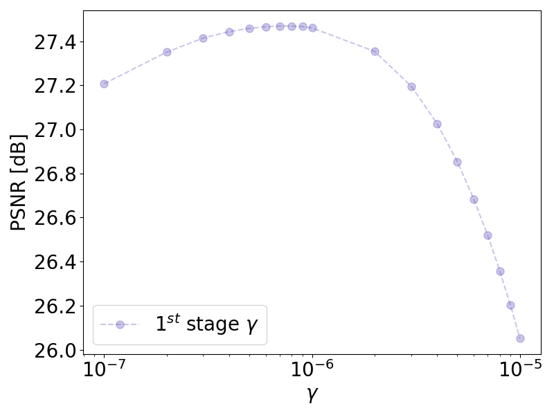
In order to reduce the amount of parameters to validate, we first fix the parameter $\gamma$ for the core stage in (24). To this aim, we have chosen to perform reconstruction with the relaxation adaption parameter $\tau$ matching the ground truth relaxation $\tau_{\mathrm{GT}}$; after this, we have performed the core stage for a set of parameters $\gamma$ in $\{i\cdot 10^{j}\colon i=0,\dots,9\wedge j=-7,-6,-5\}$. Given the outcome $A_{\gamma}\in\mathbb{R}^{2\times 2\times 50\times 50}$ of the core stage, taken their traces $u_{\gamma}=\mathrm{tr}A_{\gamma}$ and have computed the PSNR with the ground truth $u_{\mathrm{GT}}=\mathrm{tr}A_{\mathrm{GT}}$. The parameter $\gamma^{*}$ that maximizes the PSNR averaged across all phantoms has been selected as the fixed reconstruction parameter for the core stage. The average PSNR curve for the parameter $\gamma$ is plotted in figure 2(a). The maximum PSNR value corresponds to $\gamma^{*}=7\cdot 10^{-7}$. In figure 2(b) we have displayed also the average SSIM curve.

With $\gamma^{*}$ fixed, we now perform the full reconstruction varying the relaxation adaption parameter $\tau$ in the set $\{0\}\cup\{i\cdot 10^{j}\colon i=0,\dots,9\wedge j=-7,-6,-5\}$ and the starting parameter $\nu_{0}$ for the deconvolution stage in (32) in $\{10^{-5},10^{-6},10^{-7},10^{-8},10^{-9}\}$ and for $n_{\mathrm{it}}=10$ iterations. We have then computed the PSNR values between the reconstructions $\rho_{\tau,\nu_{0},n_{\mathrm{it}}}$ with the ground truth $\rho_{\mathrm{GT}}$ and selected the parameters $(\tau^{*},\nu_{0}^{*},n_{\mathrm{it}}^{*})$ that maximize the average PSNR. The values of the average PSNR for varying $\tau$ and $\nu_{0}$ (but $n_{\mathrm{it}}$) are displayed in figure 2(c). The analogous values for the average SSIM score are displayed in figure 2(d).

(a) Average PSNR curve with adaption parameter $\tau=5\cdot 10^{-6}$ coinciding with the simulated delay $\tau_{\mathrm{GT}}$, for a variety of regularization parameters $\gamma$ for the Core Stage. The maximum PSNR value corresponds to the parameter $\gamma^{*}=7\cdot 10^{-7}$.

(b) Average SSIM curve with adaption parameter $\tau=5\cdot 10^{-6}$ coinciding with the simulated delay, for a variety of regularization parameters $\gamma$ for the Core Stage.

(c) Average PSNR values of the final reconstruction for all combinations of relaxation correction parameters $\tau$ and Deconvolution Stage parameters $\nu_{0}$, with $\gamma=\gamma^{*}$ fixed for all reconstruction. In accordance with expectation, the absolute maximum value corresponds to the choice of $\tau=\tau_{\mathrm{GT}}=5\cdot 10^{-6}$. The optimal deconvolution parameter is $\nu_{0}^{*}=10^{-7}$ and $n_{\mathrm{it}}^{*}=10$.

(d) Average SSIM values of the final reconstruction for all combinations of relaxation correction parameters $\tau$ and Deconvolution Stage parameters $\nu_{0}$, with $\gamma=\gamma^{*}$ fixed for all reconstruction.

Figure 2: Overview of the average PSNR values over the simulated phantoms.

From these tables we observe that the highest PSNR score obtained for the whole reconstruction is attained when the correction parameter $\tau$ coincides with the ground truth delay $\tau_{\mathrm{GT}}=5\cdot 10^{-6}\ $\mathrm{s}\text{/}$$.

Figure 3: Reconstruction results after the MPI Core Stage (Trace) and the Deconvolution Stage (Deco.) of the 5 simulated phantoms for a variety of relaxation adaption parameters $\tau$ (rows). The ground truth delay $\tau_{\mathrm{GT}}=5\cdot 10^{-6}$ is underlined. We have diplayed the traces obtained after the MPI Core Stage with the parameter $\gamma^{*}$. The final reconstructions are obtained using the deconvolution parameter $\nu_{0}^{*}=10^{-7}$ using all entries of the MPI Core Response. We observe that the reconstructions obtained with $\tau=\tau_{\mathrm{GT}}=5\cdot 10^{-6}$ are among the closest to the ground truths and exhibit the smallest amount of artifacts.

For a qualitative underpinning of this proof of concept, we display the reconstructions obtained in figure 3. We observe that the reconstructions look closer to the ground truths when the relaxation adaption $\tau$ corresponds to the ground truth delay of $\tau_{\mathrm{GT}}=5\cdot 10^{-6}$. Moreover, we observe that when the relaxation adaption parameter $\tau$ is too small, the reconstructed traces are strongly blurred and the deconvolution does not retrieve meaningful information about the underlying distribution. On the other hand, when the adaption parameter $\tau$ is too large, one observes the increasing number of boundary effects on the final reconstructions.

Preprocessing

Core Stage

Deconvolution Stage

Phantom

AF-TF

M-TF

HPF

$\mathrm{SNR}_{x}$

$\mathrm{SNR}_{y}$

$\tau$

Reg. Ord.

CG maxit

CG tol.

$\gamma$

CG maxit

CG tol.

$n_{\mathrm{it}}$

$\nu_{0}$

% cut

% padding

Dot

$\checkmark$

$\times$

3

1

1

$10^{-6}$

2

15k

$10^{-6}$

$10^{-7}$

10k

$10^{-12}$

10

$10^{-5}$

5

5

Icecream

$\checkmark$

$\times$

2

1

1

$10^{-6}$

2

15k

$10^{-6}$

$10^{-7}$

10k

$10^{-12}$

10

$10^{-5}$

5

5

Spiral

$\checkmark$

$\times$

2

3

3

$2\cdot 10^{-6}$

2

15k

$10^{-6}$

$10^{-7}$

10k

$10^{-12}$

10

$10^{-5}$

5

5

Table 1: Overview of the parameters used in the reconstructions of the real MPI 2D data. All reconstructions have been performed on a $51\times 45$ grid discretization of the FOV using the data collected in the DF-FOV.

(a) Traces with different $\tau_{x}$ and $\tau_{y}$.

(b) Reconstructions with different $\tau_{x}$ and $\tau_{y}$.

Figure 4: Reconstruction results on the dot phantom in figure 1(a) for a variety of relaxation adaption parameters $\tau_{x}$ and $\tau_{y}$. All other parameters are fixed. We observe in figure 4(a), that when $\tau_{x}$, $\tau_{y}<10^{-6}$, the trace and the subsequent deconvolution are a blurry version of the dot phantom. Increasing the size of $\tau_{x}$, $\tau_{y}$ helps obtaining a trace and a reconstruction in which the dot-phantom is less blurred. Observing the reconstructions in figure 4(b) row-wise and column-wise suggests that increased correction in one of the channels helps obtaining less blur in that direction. On the other hand, we observe that, when the relaxation parameters $\tau_{x}$, $\tau_{y}\geq 5\cdot 10^{-6}$, reconstruction artifacts appear more strongly, the bigger the relaxation parameter.

3.3 Effect of relaxation adaption on real data

In this section reconstrcutions are performed on real data from the dataset [32]. Concerning the choice of a discretization grid, the FOV in the dataset [32] is of size $34\ $\mathrm{mm}\text{/}$\times 30$\mathrm{mm}\text{/}$$ and the usual discretization is a $17\times 15$ grid [41]. In the experiments of this section we consider a 3-fold refinement of the reconstruction grid $N_{x}\times N_{y}=51\times 43$. We note further that the FOV is larger than the drive-field field of view (DF-FOV), which is the smallest axis parallel box containing the scanning curve, where the data is collected.

3.3.1 Effect of channel-wise relaxation adaption on a real phantom.

In this second experiment we consider the dot phantom contained in figure 1(a) and study the effect of relaxation adaption. To this end we perform reconstruction using the relaxation adaption step for a set of values $\tau\in\{0,10^{-7},10^{-6},10^{-5},5\cdot 10^{-5}\}$. All other parameters of the method are fixed according to table 1. The relaxation adaption has been performed for each channel separately, so that we have corrected the $x$-channel with a relaxation parameter $\tau_{x}$ and the $y$-channel with a parameter $\tau_{y}$. In this way, the effect of the relaxation adaption on both the trace and the final deconvolution is more visible. An overview of the reconstructions is displayed in figure 4.

We observe from the traces in figure 4(a) that the effect of a lack of adaption (upper left quarter) corresponds to a blurring of the trace. This phenomenon is close to the one observed in the simulated scenario in 3. On the other hand, a relaxation adaption parameter $\tau$ which is too high, yields artifacts. From the visual results obtained in the final reconstruction in figure 4(b), it appears that the relaxation parameter that yields reconstruction that are visually similar to the underlying phantom in figure 1(a) is close to the values of $10^{-6}\ $\mathrm{s}\text{/}$$. Finally, observing the results in figure 4 row-wise (resp. column-wise), the relaxation adaption step performed channel wise, seem to have a corresponding deblurring effect on the channel’s direction. This phenomenon can be seen by inspecting any of the columns in 4(b). For each column (fixed $\tau_{y}$), increase of the parameter $\tau_{x}$ corresponds to a compression of the reconstruction along the vertical direction (corresponding to the $x$-channel). Conversely, for any fixed $\tau_{x}$, inspection of the related row shows compression of the reconstruction in the horizontal direction (corresponding to the $y$-channel). Coherently, the diagonal entries of figure 4 show similar compression of the reconstructed phantom along both directions. This indicates that the choice of a unique relaxation adaption parameter $\tau=\tau_{x}=\tau_{y}$ for both channels is sensible.

3.3.2 Effect of the relaxation adaption on further phantoms

In our last experiment, we show reconstructions on three phantoms in figure 1 and in particular, we show that the relaxation adaption step can help in reconstructing features of the underlying particle distributions that are not visible by considering simply the Langevin model. The chosen relaxation parameters as well as the preprocessing and reconstruction parameters are displayed in table 1. These parameters have been selected by visual inspection of the reconstructions obtained. The final reconstructions are displayed in figure 5. We observe that the shape and the main features of the phantoms are reconstructed.

(a) Dot, $\tau=10^{-6}$

(b) IceCream, $\tau=10^{-6}$

(c) Snail, $\tau=2\cdot 10^{-6}$

Figure 5: Reconstruction obtained with the relaxation adaption step of the three phantoms in 1 from the real data in the dataset [32]. Comparing the reconstructions with the pictures in figure 1, we observe that the shape and the main features of the phantoms are reconstructed.

To demonstrate that the reconstruction of the shapes and the features is an effect of the model and relaxation adaption step introduced in this paper, we show in figure 6 in more detail the effect of the relaxation adaption step on the components of the MPI core response $A_{1,1}$, $A_{1,2}$, $A_{2,1}$ and $A_{2,2}$, on the trace $A_{1,1}+A_{2,2}$ as well as on the final reconstruction for a variety of choices of the parameter $\tau$.

Figure 6: Detailed overview of the outputs of the MPI Core Stage and the Deconvolution Stage for a set of relaxation parameters $\tau$. We observe that, when there is no adaption ($\tau=0$) or if $\tau$ is too small (below $5\cdot 10^{-7}$), the shape of the phantom is not clearly recognizable. An increased parameter, helps recover the shape, although with various artifacts. When $\tau=2\cdot 10^{-6}$, the spiral shape of the phantom is clearly visible.

From figure 6 we observe that when the Langevin model is considered, i.e., no relaxation ($\tau=0$), the snail-like shape of the phantom in figure 1(c) is not distinguishable. The snail phantom remains indistinguishable even if relaxation correction is applied but with a parameter $\tau$ that is too small (e.g. smaller than $5\cdot 10^{-7}$). However, when the relaxation parameter $\tau$ is big enough, the snail-like shape of the phantom becomes more visible, although with artifacts. When the relaxation parameter $\tau$ reaches $10^{-6}$, the shape of the phantom is clearly visible. An interesting observation is that if $\tau$ increases slightly beyond $10^{-6}$, the reconstructed phantom is not a unique, connected piece, but shows breaking points between the junctures of the tubes constituting the phantom. This is however interesting, as the phantom in figure 1(c) is not a unique, bent and connected tube containing nanoparticles, but the junction of 5 independent tubes, disposed in a spiral pattern. From a closer inspection of the phantom in figure 1(c), there are no particles in the junctions between the tubular elements of the phantom.

4 Conclusion

In this work, we have considered a multi-dimensional Debye model to account for relaxation effects of the magnetic particles. We have obtained reconstruction formulae for this model and shown that the Debye model-based signal is related to Langevin model-based signal via a linear time-invariant system with exponential memory. We have shown that this relation, upon time discretization, implies a first-order linear recurrence to yield the corresponding Langevin model-based signal data from the measured signal data. We employed the latter to devise a relaxation-adaption step in order to provide a reconstruction algorithm. We have seen that the relaxation-adapted signal data is represented by the standard MPI core operator which allowed us to adapt our previous reconstruction scheme MoBiT-2S. Concerning computational costs, we have observed that, compared with the corresponding Langevin model based scheme, the relaxation-adaption step in proposed reconstruction scheme adds only low computational cost linear in the number of time-samples $L$ collected during a scan. We have provided numerical results for the proposed algorithmic approach for both simulated and real data. In particular, we were able to provide model-based reconstructions of fully multi-dimensional FFP data in a fully model-based setup. Neither a specific model transfer function as in the Langevin model approaches of [34, 31] nor hybrid corrections were employed. Instead, we were able to incorporate modeled relaxation effects of the particles via the Debye model to obtain reasonable reconstructions from real data.

Topics of future research include the extension of the proposed approach to further MPI setups including FFL setups as well as the extension of the mathematical analysis of the proposed method. From an algorithmic side, imposing further regularization beyond discretization is a topic to be addressed when dealing with more general setups.

References

- [1] B. Gleich and J. Weizenecker, “Tomographic imaging using the nonlinear response of magnetic particles,” Nature, vol. 435, pp. 1214–1217, Jun 2005.
- [2] T. Knopp and T. M. Buzug, Magnetic Particle Imaging: An Introduction to Imaging Principles and Scanner Instrumentation. Springer, 2012.
- [3] J. Weizenecker, B. Gleich, J. Rahmer, H. Dahnke, and J. Borgert, “Three-Dimensional Real-Time in Vivo Magnetic Particle Imaging,” Phys. Med. Biol., vol. 54, pp. L1–L10, 2009.
- [4] M. Irfan and N. Dogan, “Comprehensive evaluation of magnetic particle imaging (mpi) scanners for biomedical applications,” IEEE Access, vol. 10, pp. 86718–86732, 2022.
- [5] G. Song, M. Chen, Y. Zhang, L. Cui, H. Qu, X. Zheng, M. Wintermark, Z. Liu, and J. Rao, “Janus Iron Oxides @ Semiconducting Polymer Nanoparticle Tracer for Cell Tracking by Magnetic Particle Imaging,” Nano Letters, vol. 18, pp. 182–189, Jan 2018.
- [6] J. J. Connell, P. S. Patrick, Y. Yu, M. F. Lythgoe, and T. L. Kalber, “Advanced Cell Therapies: Targeting, Tracking and Actuation of Cells with Magnetic Particles,” Regenerative medicine, vol. 10, pp. 757–72, 2015.
- [7] P. Goodwill and S. Conolly, “Multidimensional X-space magnetic particle imaging,” IEEE Trans. Med. Imaging, vol. 30, pp. 1581–1590, 2011.
- [8] K. O. Jung, H. Jo, J. H. Yu, S. S. Gambhir, and G. Pratx, “Development and MPI Tracking of Novel Hypoxia-Targeted Theranostic Exosomes,” Biomaterials, vol. 177, pp. 139–148, 2018.
- [9] J. E. Lemaster, F. Chen, T. Kim, A. Hariri, and J. V. Jokerst, “Development of a Trimodal Contrast Agent for Acoustic and Magnetic Particle Imaging of Stem Cells,” ACS Applied Nano Materials, vol. 1, pp. 1321–1331, Mar 2018.
- [10] A. Tomitaka, H. Arami, S. Gandhi, and K. M. Krishnan, “Lactoferrin Conjugated Iron Oxide Nanoparticles for Targeting Brain Glioma Cells in Magnetic Particle Imaging,” Nanoscale, vol. 7, pp. 16890–16898, 2015.
- [11] J. Franke, N. Baxan, H. Lehr, U. Heinen, S. Reinartz, J. Schnorr, M. Heidenreich, F. Kiessling, and V. Schulz, “Hybrid MPI-MRI System for Dual-Modal In Situ Cardiovascular Assessments of Real-Time 3D Blood Flow Quantification - A Pre-Clinical In Vivo Feasibility Investigation,” IEEE Transactions on Medical Imaging, vol. 39, no. 12, pp. 4335–4345, 2020.
- [12] A. C. Bakenecker, M. Ahlborg, C. Debbeler, C. Kaethner, T. M. Buzug, and K. Lüdtke-Buzug, “Magnetic Particle Imaging in Vascular Medicine,” Innovative Surgical Sciences, vol. 3, no. 3, pp. 179–192, 2018.
- [13] W. Tong, H. Hui, W. Shang, Y. Zhang, F. Tian, Q. Ma, X. Yang, J. Tian, and Y. Chen, “Highly Sensitive Magnetic Particle Imaging of Vulnerable Atherosclerotic Plaque with Active Myeloperoxidase-Targeted Nanoparticles,” Theranostics, vol. 11, pp. 506–521, 2021.
- [14] S. Vaalma, J. Rahmer, N. Panagiotopoulos, R. L. Duschka, J. Borgert, J. Barkhausen, F. M. Vogt, and J. Haegele, “Magnetic Particle Imaging (MPI): Experimental Quantification of Vascular Stenosis Using Stationary Stenosis Phantoms,” PLOS ONE, vol. 12, pp. 1–22, 01 2017.
- [15] C. Billings, M. Langley, G. Warrington, F. Mashali, and J. A. Johnson, “Magnetic Particle Imaging: Current and Future Applications, Magnetic Nanoparticle Synthesis Methods and Safety Measures,” International Journal of Molecular Sciences, vol. 22, no. 14, 2021.
- [16] X. Yang, G. Shao, Y. Zhang, W. Wang, Y. Qi, S. Han, and H. Li, “Applications of Magnetic Particle Imaging in Biomedicine: Advancements and Prospects,” Front Physiol, vol. 13, p. 898426, jul 2022.
- [17] A. Güngör, B. Askin, D. A. Soydan, C. Barış Top, and T. Cukur, “Deep Learned Super Resolution of System Matrices for Magnetic Particle Imaging,” in 2021 43rd Annual International Conference of the IEEE Engineering in Medicine & Biology Society (EMBC), pp. 3749–3752, 2021.
- [18] F. Schrank, D. Pantke, and V. Schulz, “Deep learning MPI Super-Resolution by Implicit Representation of the System Matrix,” vol. 8, 2022.
- [19] L. Yin, H. Guo, P. Zhang, Y. Li, H. Hui, Y. Du, and J. Tian, “System Matrix Recovery Based on Deep Image Prior in Magnetic Particle Imaging,” Physics in Medicine & Biology, vol. 68, p. 035006, jan 2023.
- [20] K. Scheffler, M. Boberg, and T. Knopp, “Boundary Artifact Reduction by Extrapolating System Matrices Outside the Field-of-View in Joint Multi-Patch MPI,” International journal on magnetic particle imaging, vol. 8, no. 1, Suppl 1, p. 2203019, 2022.
- [21] K. Scheffler, M. Boberg, and T. Knopp, “Extrapolation of System Matrices in Magnetic Particle Imaging,” IEEE Transactions on Medical Imaging, vol. 42, no. 4, pp. 1121–1132, 2023.
- [22] T. Knopp and A. Weber, “Sparse reconstruction of the magnetic particle imaging system matrix,” IEEE Trans. Med. Imaging, vol. 32, no. 8, pp. 1473 – 1480, 2013.
- [23] A. Weber and T. Knopp, “Reconstruction of the Magnetic Particle Imaging System Matrix Using Symmetries and Compressed Sensing,” Advances in Mathematical Physics, vol. 2015, p. 460496, Oct 2015.
- [24] M. Erbe, Field Free Line Magnetic Particle Imaging. Springer, 01 2014.
- [25] V. Gapyak, T. März, and A. Weinmann, “Reconstruction Formulae for 3D Field-Free Line Magnetic Particle Imaging,” SIAM Journal on Applied Mathematics, vol. 85, no. 4, pp. 1643–1666, 2025.
- [26] D. Jiles, Introduction to Magnetism and Magnetic Materials. CRC press, 1998.
- [27] P. Goodwill and S. Conolly, “The X-Space Formulation of the Magnetic Particle Imaging Process: 1-D Signal, Resolution, Bandwidth, SNR, SAR, and Magnetostimulation,” IEEE Trans. Med. Imaging, vol. 29, pp. 1851–1859, 2010.
- [28] A. A. Ozaslan, A. Alacaoglu, O. B. Demirel, T. Çukur, and E. U. Saritas, “Fully automated gridding reconstruction for non-cartesian x-space magnetic particle imaging,” Physics in Medicine & Biology, vol. 64, p. 165018, 8 2019.
- [29] T. März and A. Weinmann, “Model-Based Reconstruction for Magnetic Particle Imaging in 2D and 3D,” Inverse Problems & Imaging, vol. 10, no. 4, pp. 1087–1110, 2016.
- [30] V. Gapyak, T. März, and A. Weinmann, “Variational Model-Based Reconstruction Techniques for Multi-Patch Data in Magnetic Particle Imaging,” Journal of Computational and Applied Mathematics, vol. 451, p. 116046, 2024.
- [31] V. Gapyak, T. März, and A. Weinmann, “Fast trajectory-independent model-based reconstruction algorithm for multi-dimensional magnetic particle imaging,” Physics in Medicine & Biology, vol. 70, p. 235028, dec 2025.
- [32] T. Knopp and K. Scheffler, “Mpidata: Equilibriummodelwithanisotropy,” 2024.
- [33] L. Li, Y. Liao, Q. Wang, Z. Zhang, D. Ge, J. Hu, N. He, Y. Liu, C. Xu, Y. Gao, P. Guo, H. Hui, X. Feng, S. Zhu, and J. Tian, “Transverse mnp signal-based isotropic imaging for magnetic particle imaging,” IEEE Transactions on Instrumentation and Measurement, vol. 73, pp. 1–13, 2024.
- [34] C. Droigk, M. Maass, and A. Mertins, “Direct multi-dimensional Chebyshev polynomial based reconstruction for magnetic particle imaging,” Physics in Medicine & Biology, vol. 67, p. 045014, feb 2022.
- [35] C. Droigk, D. H. Durán, M. Maass, T. Knopp, and K. Scheffler, “Efficient chebyshev reconstruction for the anisotropic equilibrium model in magnetic particle imaging,” 2025.
- [36] T. Sanders, J. Konkle, O. C. Sehl, A. Rahman Mohtasebzadeh, J. M. Greve, and P. W. Goodwill, “A physics-based computational forward model for efficient image reconstruction in magnetic particle imaging,” IEEE Transactions on Medical Imaging, vol. 44, no. 5, pp. 2319–2329, 2025.
- [37] J. Rahmer, J. Weizenecker, B. Gleich, and J. Borgert, “Signal Encoding in Magnetic Particle Imaging: Properties of the System Function,” BMC Medical Imaging, vol. 9, p. 4, 2009.
- [38] W. Erb, A. Weinmann, M. Ahlborg, C. Brandt, G. Bringout, T. M. Buzug, J. Frikel, C. Kaethner, T. Knopp, T. März, et al., “Mathematical analysis of the 1d model and reconstruction schemes for magnetic particle imaging,” Inverse Problems, vol. 34, no. 5, p. 055012, 2018.
- [39] P. Maaß and A. Mertins, “On the Representation of Magnetic Particle Imaging in Fourier Space,” Int J Mag Part Imag, vol. 6, no. 1, 2020.
- [40] T. Knopp, S. Biederer, T. F. Sattel, J. Rahmer, J. Weizenecker, B. Gleich, J. Borgert, and T. M. Buzug, “2D model-based reconstruction for Magnetic Particle Imaging,” Medical Physics, vol. 37, pp. 485–491, 2010.
- [41] M. Maass, T. Kluth, C. Droigk, H. Albers, K. Scheffler, A. Mertins, and T. Knopp, “Equilibrium Model With Anisotropy for Model-Based Reconstruction in Magnetic Particle Imaging,” IEEE Transactions on Computational Imaging, vol. 10, pp. 1588–1601, 2024.
- [42] L. R. Croft, P. W. Goodwill, and S. M. Conolly, “Relaxation in X-Space Magnetic Particle Imaging,” IEEE Trans Med Imaging, vol. 31, pp. 2335–2342, sep 2012.
- [43] M. I. Shliomis, “Magnetic fluids,” Soviet Physics Uspekhi, vol. 17, p. 153, feb 1974.
- [44] K. Bente, M. Weber, M. Graeser, T. F. Sattel, M. Erbe, and T. M. Buzug, “Electronic Field Free Line Rotation and Relaxation Deconvolution in Magnetic Particle Imaging,” IEEE Transactions on Medical Imaging, vol. 34, no. 2, pp. 644–651, 2015.
- [45] M. Utkur, Y. Muslu, and E. U. Saritas, “Relaxation-based viscosity mapping for magnetic particle imaging,” IOP Phys. in Med. & Biol., vol. 62, p. 3422, 4 2017.
- [46] Y. Muslu, M. Utkur, O. B. Demirel, and E. U. Saritas, “Calibration-free relaxation-based multi-color magnetic particle imaging,” IEEE Transactions on Medical Imaging, vol. 37, no. 8, pp. 1920–1931, 2018.
- [47] T. Kluth, “Mathematical models for magnetic particle imaging,” Inverse Problems, vol. 34, no. 8, p. 083001, 2018.
- [48] W. T. Coffey, P. J. Cregg, and Y. U. P. Kalmykov, On the Theory of Debye and Néeel Relaxation of Single Domain Ferromagnetic Particles, pp. 263–464. John Wiley & Sons, Ltd, 1992.
- [49] L. Néel, “Thermoremanent magnetization of fine powders,” Rev. Mod. Phys., vol. 25, pp. 293–295, 01 1953.
- [50] H. Risken, The Fokker-Planck Equation: Methods of Solution and Applications. Springer series in synergetics, Springer-Verlag, 1989.
- [51] S. Solibida, D. Pantke-Stratmann, F. Schrank, and V. Schulz, “A refined debye model for the dynamic magnetization response of superparamagnetic nanoparticles,” Int J Mag Part Imag, vol. 9, no. 1, 2023.
- [52] Y. Li, P. Zhang, X. Feng, H. Hui, and S. Tian, “Multi-dimensional debye model for nanoparticle magnetization in magnetic particle imaging,” Int J Mag Part Imag, vol. 9, no. 1, 2023.
- [53] Y. Li, H. Hui, P. Zhang, J. Zhong, L. Yin, H. Zhang, B. Zhang, Y. An, and J. Tian, “Modified jiles-atherton model for dynamic magnetization in x-space magnetic particle imaging,” IEEE Transactions on Biomedical Engineering, vol. 70, no. 7, pp. 2035–2045, 2023.
- [54] V. Gapyak, T. März, and A. Weinmann, “Towards addressing nanoparticle relaxation in model-based reconstruction,” Int. J. Mag. Par. Imag., 2026. Accepted for Publication.
- [55] K. E. Atkinson, “The numerical solution of fredholm integral equations of the second kind,” SIAM Journal on Numerical Analysis, vol. 4, no. 3, pp. 337–348, 1967.
- [56] V. Gapyak, T. März, and A. Weinmann, “Quality-Enhancing Techniques for Model-Based Reconstruction in Magnetic Particle Imaging,” Mathematics, vol. 10, no. 18, 2022.
- [57] T. März, V. Gapyak, and A. Weinmann, “Higher order regularization using harmonic eigenfunctions for model-based reconstruction in magnetic particle imaging,” Inverse Problems, vol. 42, p. 025002, feb 2026.
- [58] T. März, V. Gapyak, and A. Weinmann, “A Flexible Model-Based Regularized Reconstruction Approach for Magnetic Particle Imaging,” AIP Conf. Proc., vol. 3094, p. 440001, 06 2024.
- [59] S. V. Venkatakrishnan, C. A. Bouman, and B. Wohlberg, “Plug-and-Play Priors for Model Based Reconstruction,” in 2013 IEEE Global Conference on Signal and Information Processing, pp. 945–948, 2013.
- [60] K. Zhang, Y. Li, W. Zuo, L. Zhang, L. Van Gool, and R. Timofte, “Plug-and-Play Image Restoration With Deep Denoiser Prior,” IEEE Transactions on Pattern Analysis and Machine Intelligence, vol. 44, no. 10, pp. 6360–6376, 2022.