TimeSqueeze: Dynamic Patching for Efficient Time Series Forecasting

Abstract

Transformer-based time series foundation models face a fundamental trade-off in choice of tokenization: point-wise embeddings preserve temporal fidelity but scale poorly with sequence length, whereas fixed-length patching improves efficiency by imposing uniform boundaries that may disrupt natural transitions and blur informative local dynamics. In order to address these limitations, we introduce TimeSqueeze, a dynamic patching mechanism that adaptively selects patch boundaries within each sequence based on local signal complexity. TimeSqueeze first applies a lightweight state-space encoder to extract full-resolution point-wise features, then performs content-aware segmentation by allocating short patches to information-dense regions and long patches to smooth or redundant segments. This variable-resolution compression preserves critical temporal structure while substantially reducing the token sequence presented to the Transformer backbone. Specifically for large-scale pretraining, TimeSqueeze attains up to $20\times$ faster convergence and $8\times$ higher data efficiency compared to equivalent point-token baselines. Experiments across long-horizon forecasting benchmarks show that, TimeSqueeze consistently outperforms comparable architectures that use either point-wise tokenization or fixed-size patching.

1 Introduction

Accurate time-series forecasting is crucial across numerous domains, including energy, finance, climate, and healthcare. Historically, forecasting has relied on narrow, task-specific statistical models; however, recent advances in deep learning have enabled the development of versatile, generalist models capable of cross-domain transfer. In particular, time-series foundation models trained on heterogeneous datasets offer flexible zero-shot and few-shot generalization across a wide range of forecasting tasks.

Effective pretraining of these foundation models necessitates modeling long historical contexts, often extending to thousands of timesteps, which creates formidable computational and memory constraints. Recent studies demonstrate that increasing context length during pretraining yields substantial improvements in downstream inference performance  (Gao et al., 2024; Liu et al., 2024). Therefore, designing architectures that remain scalable and computationally efficient under long-context regimes is imperative for realizing the full potential of time series foundation models.

Central to addressing these scalability challenges is the design of an efficient tokenizer that effectively represents input signals in an embedding space while managing computational complexity. Current approaches predominantly adopt one of two strategies. The first approach involves independently encoding each time point (Zhou et al., 2021; Wu et al., 2021; Zhou et al., 2022; Ansari et al., 2024; Shi et al., 2024), which preserves fine-grained temporal variations and accommodates data of arbitrary frequency and seasonality. However, this point-wise encoding strategy suffers from limited scalability as sequence length increases, which is precisely the bottleneck that impedes long-context pretraining. The second approach, pioneered by Nie et al. (2022) and subsequently adopted by numerous transformer-based forecasting models  (Goswami et al., 2024; Das et al., 2024; Woo et al., 2024; Liu et al., 2024, 2025), employs fixed-size patching to compress multiple consecutive time points into a single embedding. While this patching strategy significantly enhances computational scalability, it introduces some limitations that compromise its effectiveness. First, determining the optimal patch size is non-trivial and heavily dependent on dataset-specific characteristics such as sampling frequency and seasonal patterns, typically requiring empirical evaluation across different patch sizes for each dataset. Second, and perhaps more critically, many time series exhibit heterogeneous information density across different temporal regions, with some segments displaying rapid variations while others remaining relatively stable. This temporal heterogeneity renders uniform patching suboptimal, as it fails to adapt the representational granularity to the local complexity of the signal.

Motivated by these requirements, we propose TimeSqueeze, a hybrid time-series tokenization that combines the expressive power of point-embeddings with the computational efficiency of patch-embeddings. First, a lightweight state space model (SSM) (Gu and Dao, 2023) based encoder extracts local fine-grained features at full resolution. Then, a dynamic patching module groups these embeddings into patches of varying sizes, allocating smaller patches to information-rich regions and larger patches to redundant ones, yielding a variable-resolution representation. This results in significantly fewer tokens for the transformer backbone while preserving salient temporal dynamics, thereby overcoming fixed patch size limitations and enabling scalable, high-fidelity modeling.

Our contributions are as follows:

• We propose TimeSqueeze, a hybrid tokenizer with an efficient SSM-based encoder–decoder that preserves fine-grained long-context features while enabling content-aware, truly dynamic patching via adaptive downsampling.

• We establish that TimeSqueeze integrates seamlessly with various Transformer backbones, enabling pretraining of large-scale time series foundation models with substantially reduced training budgets.

• We demonstrate that TimeSqueeze achieves performance on par with state-of-the-art point embedding models while delivering up to $20\times$ faster training and $8\times$ higher pre-training data efficiency.

• We evaluate TimeSqueeze across diverse backbones and pretraining datasets, showing consistent gains over prior patching and tokenization methods in both zero-shot and full-shot settings on univariate and multivariate forecasting tasks.

2 Related Works.

Long-sequence architectures. While Transformer architectures (Vaswani et al., 2017) have shown strong time series forecasting performance due to their expressivity and flexibility, their quadratic computational and memory complexity with respect to sequence length limits their scalability to long historical contexts. Innovations such as (Li et al., 2019; Wu et al., 2021; Zhou et al., 2021) have adapted Transformers for long-term forecasting, but pretraining on extremely long contexts remains challenging. Recently, time-series foundation models have demonstrated scalability to long contexts supporting arbitrary forecasting horizons, while Time-MoE (Shi et al., 2024) leveraged Mixture-of-Experts routing to enable the first billion-parameter model with tractable inference. Despite these advances, the cost of long-context pretraining remains high due to the underlying Transformer backbone. Although SSM architectures handle long contexts more efficiently, they remain underexplored for time series forecasting, highlighting the need for scalable methods for efficient long-context processing.

Patch-based tokenization. Introduced in PatchTST (Nie et al., 2022), patch-based compression has emerged as a fundamental technique for scaling time series foundation models. By embedding contiguous sub-sequences (patches) rather than individual time points, this approach reduces the effective sequence length while preserving essential local temporal patterns. Subsequent foundation models, including TimesFM (Das et al., 2024), Moment (Goswami et al., 2024), Moirai (Woo et al., 2024), and Timer-XL (Liu et al., 2024), have adopted this paradigm, collectively demonstrating that patching enables more efficient training and inference. However, these approaches utilize a fixed patch size for a given sequence, limiting their application to real-world data with high temporal variance, underscoring the need for dynamic, data-driven compression strategies that can adjust patching to varying temporal structures within a series.

Dynamic patching in time-series modeling. Several recent methods explored the idea of adapting the patch size based on input automatically, instead of hand-crafted heuristics. HDMixer (Huang et al., 2024) enables extension of patch size by selectively combining adjoining fixed-size patches. IMTS (Zhang et al., 2024) is tailored to irregularly sampled series, where the patch size is adjusted dynamically in order to maintain the same number of temporal observations within each patch. LightGTS (Wang et al., 2025) adjusts the patch size for each input signal based on periodicity in the Fourier domain and SRSNet (Wu et al., 2025a) introduces a dynamic selection and combining of features to improve the forecasting capability. However, none of these methods perform within-sequence dynamic patching that relocates patch boundaries and varies patch sizes inside each series based on local signal statistics. More recently, EntroPE (Abeywickrama et al., 2025) introduces entropy based patching of the input time series but requires discretizing the input and learning a separate model for entropy calculation, adding additional overhead.

Insights from language modeling. Similar challenges arise in large language models (LLMs), where the choice of input representation has a direct impact on scalability and fidelity. Conventional tokenization introduces systematic biases and brittle dependencies, motivating tokenizer-free models that operate at the byte level. Yet, naïve byte-level processing leads to prohibitively long input sequences (Slagle, 2024), straining attention-based architectures. To overcome this, adaptive compression techniques have been proposed. The Byte Latent Transformer (BLT) dynamically merges predictable byte spans into compact latent tokens using entropy-guided segmentation (Pagnoni et al., 2024), while H-Net (Hwang et al., 2025), inspired by U-Net (Ronneberger et al., 2015) and its broad adaptation in vision (Child, 2021; Ho et al., 2020; Wu et al., 2025b), compresses and reconstructs sequences in various resolutions, and uses a state-space model for more efficient byte-level processing. These approaches highlight a key principle: efficiency and accuracy can be jointly achieved by allocating higher granularity to information-dense regions and applying more aggressive compression where redundancy dominates.

3 Methodology

In this work, we will mainly focus on the task of designing an efficient tokenizer for time-series forecasting foundation models and refer to the combined model as TimeSqueeze from here on for simplicity.

Problem Statement. The fundamental objective in time-series forecasting is to predict future values based on historical observations. Given a sequence of $T$ historical data points, $\mathbf{X}_{1:T}=(x_{1},x_{2},\ldots,x_{T})\in\mathbb{R}^{T}$, the goal is to estimate the next $H$ values of the series. This is formalized via a model $f_{\theta}$ that maps the historical context to future predictions, i.e., $\hat{\mathbf{X}}_{T+1:T+H}=f_{\theta}(\mathbf{X}_{1:T})\in\mathbb{R}^{H}$. Adopting the channel independence principle of Nie et al. (2022), the model can flexibly process multivariate time series by decomposing inputs into collections of univariate series. This general formulation enables time-series foundation models to address forecasting tasks with arbitrary input dimensionality, thereby supporting broad applicability across diverse, real-world domains. Note that we also consider explicit modeling of multivariate forecasting in section 6.

Figure 1: Architectural overview of TimeSqueeze forecasting model. An SSM encoder first processes the raw series at full resolution to extract fine-grained features. Dynamic patching then adaptively compresses the sequence, selecting the salient subset of features. A Transformer backbone performs contextual modeling on the downsampled features, and an unpatching module upsamples the signal to the original resolution while preserving causality. Finally, an SSM decoder combines the compressed and fine-grained features, passing the hybrid features to multi-horizon heads, thereby improving efficiency without sacrificing temporal fidelity.

3.1 Architectural Overview

To combine the expressivity of point-embeddings with the computational efficiency of patch embeddings, TimeSqueeze employs a hybrid multi-resolution architecture with four key components: (1) a lightweight encoder-decoder pair operating at full input resolution to capture fine-grained local features, (2) adaptive patching modules that dynamically compute salient features for efficient downsampling and upsampling, (3) a decoder-only mixture-of-experts (MoE) Transformer backbone for modeling causal dependencies at scale, and (4) a multi-horizon forecasting head that jointly optimizes predictions across multiple time horizons to support both short- and long-term forecasting, as shown in Figure 1. The first two components together form the hybrid tokenization mechanism in TimeSqueeze.

Formally, the end-to-end model can be described as

$$H_{1:T} =\mathcal{E}(X_{1:T}),\quad Z_{1:P}=\mathcal{M}\!\left(\mathcal{P}(H_{1:T})\right),$$ (1)

$$Y_{1:T} =\mathcal{D}\!\left(H_{1:T},\mathcal{U}(Z_{1:P})\right)$$

where $\mathcal{E}$ is the encoder, $\mathcal{P}$ is the patching module, $\mathcal{M}$ is the MoE Transformer backbone, $\mathcal{U}$ is the unpatching module, and $\mathcal{D}$ is the decoder. Here, $X_{1:T}\in\mathbb{R}^{T}$ denotes the original input sequence, $H_{1:T}\in\mathbb{R}^{T\times D}$ denotes the $D$-dimensional encoder embeddings, $Z_{1:P}\in\mathbb{R}^{P\times D}$ denotes the patch-level latent representation after $\mathcal{P}$ and $\mathcal{M}$, and $Y_{1:T}\in\mathbb{R}^{T\times D}$ denotes the decoder embeddings that serve as the final representation for downstream forecasting.

3.1.1 State-Space Encoder and Decoder

The encoder and decoder modules operate directly on input time series at native resolution to preserve fine-grained temporal details essential for accurate forecasting, particularly in high-frequency data. To handle long, uncompressed sequences efficiently while generating representations suitable for subsequent patching, both modules are constructed using Mamba layers (Gu and Dao, 2023).

Mamba offers nearly linear computational scaling with respect to sequence length, enabling extraction of intricate local patterns from extended contexts by the encoder, without the quadratic complexity of traditional Transformer architectures. Further, the decoder uses the same architecture to efficiently combines outputs from the Transformer backbone with residual embeddings from the encoder to produce final representations for forecasting, creating a rich multi-scale feature space that captures both local fine-grained patterns and global contextual dependencies.

3.1.2 Dynamic Patching and Unpatching

After the encoder produces fine-grained representations, the patching module compresses the sequence of embeddings before passing them to the Transformer backbone. The objective is to allocate computational resources efficiently by employing a dynamic patching strategy that adapts to the local complexity of the input signal. This strategy forms larger patches to compress regions of low information density while using smaller patches to preserve detail in regions of high information content (Appendix J).

Patching. Unlike language models that operate on discrete token sequences, time series data often exist in continuous space and exhibit rich statistical properties. This continuous nature makes time series particularly amenable to characterization via statistical measures such as local variance or power, without relying on external metrics for guidance (Pagnoni et al., 2024). We leverage this by tracking the absolute difference between consecutive samples, comparing it to the average signal power within a predetermined lookback window, and then computing the patch boundaries in the original signal space rather than the embedding space. Formally, we maintain a sliding window $\mathcal{W}_{i}=\{x_{i-L},\ldots,x_{i-1}\}$ of length $L$ to compute the local average power as

$$P_{i}=\frac{1}{L}\sum_{j=i-L}^{i-1}x_{j}^{2}.$$

Our adaptive patching mechanism declares a patch boundary at timestep $i$ if the absolute difference between consecutive samples exceeds a threshold scaled by the local power, which we refer to as relative deviation-based patching:

$$b_{i}=\begin{cases}1&\text{if }|x_{i}-x_{i-1}|>\tau\sqrt{P_{i}}\\ 0&\text{otherwise}\end{cases}.$$

Here, $\tau>0$ is a tunable threshold parameter controlling patch sensitivity and the average compression ratio. Using $\sqrt{P_{i}}$ normalizes the threshold with respect to signal amplitude, allowing the method to adapt dynamically across varying signal magnitudes and variances. Intuitively, can be thought of as locating the points of significant local change, where a new patch should begin so that the SSM embedding/token at the patch boundary can adequately summarize the upcoming region. Once patch boundaries are determined, the embeddings within each patch are compressed by retaining only the boundary embeddings and discarding intermediate ones (Figure 1). Note that retaining only the boundary embeddings helps preserve causality for the subsequent unpatching step.

Unpatching. The unpatching module restores the compressed embeddings to the original sequence length while maintaining causal consistency. After backbone processing of boundary embeddings, each updated embedding is repeated across all timesteps within its corresponding patch and passed to the decoder for upsampling. Since boundary embeddings represent the start of each patch, the reconstructed output at timestep $t$ depends only on inputs from times $\leq t$, preventing leakage of future information.

Positional Information. Unlike language models, which predict the next discrete token, time series foundation models demand more nuanced objective during pretraining. For instance, forecasting must occur at a specified frequency within the original continuous signal space, not within the compressed embedding space. Prior works on tokenizer-free language modeling, such as BLT (Pagnoni et al., 2024) and Dynamic Chunking (Hwang et al., 2025), do not retain the original positional indices and restrict the attention mechanism to relative positional information post-downsampling. In contrast, TimeSqueeze explicitly preserves the position IDs of embeddings before downsampling and utilizes these absolute positions to compute attention after compression.

3.1.3 Mixture-of-Experts Transformer Backbone

Due to its modular design, our hybrid feature extraction framework is compatible with any existing time-series forecasting backbone. In this work, we adopt the Time-MoE backbone (Shi et al., 2024), a scalable decoder-only Transformer augmented with a sparse MoE routing mechanism. Time-MoE incorporates several enhancements to improve training stability and forecast accuracy: it employs RMSNorm for layer normalization and replaces absolute positional encoding with Rotary Positional Embeddings (RoPE), facilitating better handling of variable sequence lengths and improved extrapolation. Following established design patterns, the standard feed-forward network (FFN) is replaced by an MoE layer containing a pool of $N$ non-shared experts alongside one shared expert that consolidates common knowledge. For each input token, a routing mechanism selects the top $K$ non-shared experts to process the signal, enabling efficient scaling to billions of parameters while maintaining manageable inference costs.

3.1.4 Multi-horizon forecasting

To enhance forecasting flexibility and robustness, we employ a multi-horizon forecasting head as introduced in (Shi et al., 2024). This approach enables simultaneous prediction across multiple future horizons rather than restricting the model to a single forecast length. Specifically, it consists of multiple single-layer FFNs, each dedicated to a distinct forecasting horizon. The model is trained using a composite loss aggregating errors from all horizons, which improves generalization. During inference, a simple scheduling strategy selects the appropriate horizon-specific output, enabling the model to produce forecasts of arbitrary length flexibly.

3.2 Model Training

Pretraining Dataset. Efficient pretraining of a foundation model necessitates a large and diverse dataset. For this purpose, we employ the Time-300B dataset (Shi et al., 2024), a high-quality, open-access dataset composed of time series from numerous public sources across various sectors, including weather, transportation, and finance, which is further expanded with synthetic data. It consists of a broad range of frequencies, ranging from seconds to yearly, and a massive scale of over 300 billion time points, making it well-suited for pretraining large-scale models.

Loss Formulation. Following (Shi et al., 2024), our training objective is a composite loss function that combines a primary forecasting loss with an auxiliary term for load balancing, which enables a fair comparison against the point-embedding baseline Time-MoE. The primary auto-regressive loss, $\mathcal{L}_{\text{ar}}$, is the Huber Loss (Huber, 1992), chosen for its robustness against outliers:

$$\mathcal{L}_{ar}(x_{t},\hat{x}_{t})=\begin{cases}\frac{1}{2}(x_{t}-\hat{x}_{t})^{2},&\text{if }|x_{t}-\hat{x}_{t}|\leq\delta,\\ \delta\left(|x_{t}-\hat{x}_{t}|-\frac{1}{2}\delta\right),&\text{otherwise,}\end{cases}$$ (2)

where $\delta$ is a hyperparameter that balances the quadratic ($L_{2}$) and linear ($L_{1}$) penalties.

To ensure balanced expert utilization and prevent routing collapse, we incorporate an auxiliary loss, $\mathcal{L}_{\text{aux}}$, as proposed in (Fedus et al., 2022):

$$\mathcal{L}_{\text{aux}}=N\sum_{i=1}^{N}f_{i}r_{i},$$ (3)

where $f_{i}$ is the fraction of tokens dispatched to expert $i$, and $r_{i}$ is the average router probability assigned to the expert. The final training loss, $\mathcal{L}$, averages the auto-regressive loss across $K$ multi-resolution projections and combines it with the weighted auxiliary loss:

$$\mathcal{L}=\frac{1}{K}\sum_{j=1}^{K}\mathcal{L}_{\text{ar}}\left(\mathbf{X}_{t+1:t+p_{j}},\hat{\mathbf{X}}_{t+1:t+p_{j}}\right)+\alpha\mathcal{L}_{\text{aux}},$$ (4)

where $p_{j}$ is the forecast horizon for the $j$-th projection and $\alpha$ is a scaling coefficient.

Model Configuration. We consider two model sizes in this work, demonstrating the scalability of our approach. TimeSqueeze ${}_{\text{base}}$ has a total of 117M parameters with 54M active parameters, while TimeSqueeze ${}_{\text{large}}$ contains 469M total parameters with 216M active parameters. Both models are trained for 100,000 steps with a batch size of 256 and a maximum context length of 2048, corresponding to 500K time points per iteration and a total of 50B time steps during pretraining. Finally, for the patching and unpatching modules, we target an average compression rate of 4 in TimeSqueeze by setting the threshold factor $\tau=0.3$, and limiting the maximum patch size to $8$, resulting in an average compression ratio of $4\times$ on the pretraining dataset, balancing computational savings and information preservation. During inference, we use the same $\tau$ across all datasets, demonstrating the robustness of $\tau$. Further configuration details are provided in Appendix B.

4 Experimental Results

We aim to demonstrate that TimeSqueeze improves both efficiency and forecasting performance over point-embedding models by dynamically compressing the input context under a fixed computational budget. We adopt Time-MoE as our evaluation backbone due to the public availability of its pretraining pipeline and dataset. In our implementation, we keep the forecasting backbone and all training settings unchanged, and modify only the tokenization stage: we replace Time-MoE’s SwiGLU-based point-wise tokenizer with our SSM-based dynamic patching module. This controlled setup isolates the effect of dynamic context compression and enables a fair comparison between the two models.

Baselines. We use Time-MoE as our baseline, and pretrain TimeSqueeze following the training scheme of (Shi et al., 2024), but using $8\times$ lesser data and $\approx 20\times$ less train time, as shown in Figure 2(a). We forecast on four prediction horizons $\{96,192,336,720\}$ but use the same context length of $512$ in all cases. While, we study the point-forecasting performance of TimeSqueeze, but it can easily be extended to provide probabilistic forecasts by substituting the model’s linear projection head with a probabilistic head. We assess model performance using the mean squared error (MSE) and mean absolute error (MAE), computed between the predicted values and the ground truth. For completeness, we also compare against Moirai-large (Woo et al., 2024), TimesFM (Das et al., 2024), Moment (Ansari et al., 2024), and Chronos (Goswami et al., 2024), with results taken from (Shi et al., 2024).

Table 1: Performance comparison of zero-shot forecasting. Best results are highlighted in red and second-best in blue.

Models	Metrics	TimeSqueeze ${}_{\text{base}}$		TimeSqueeze ${}_{\text{large}}$		Time-MoE${}_{\text{base}}$		Time-MoE${}_{\text{large}}$		Moirai${}_{\text{base}}$		TimesFM		Moment		Chronos${}_{\text{large}}$
		MSE	MAE	MSE	MAE	MSE	MAE	MSE	MAE	MSE	MAE	MSE	MAE	MSE	MAE	MSE	MAE
ETTh1	96	$0.359$	$0.385$	$0.360$	0.379	0.357	$0.381$	0.350	$0.382$	$0.376$	$0.392$	$0.414$	$0.404$	$0.688$	$0.557$	$0.441$	$0.390$
	192	$0.400$	0.410	$0.402$	$0.407$	0.388	$0.412$	0.384	$0.404$	$0.417$	$0.413$	$0.465$	$0.434$	$0.688$	$0.560$	$0.502$	$0.424$
	336	0.420	$0.423$	$0.423$	0.412	0.411	$0.430$	0.411	$0.434$	$0.433$	0.428	$0.503$	$0.456$	$0.675$	$0.563$	$0.576$	$0.467$
	720	0.428	0.446	$0.441$	$0.448$	0.427	$0.455$	$0.449$	$0.477$	$0.447$	0.444	$0.511$	$0.481$	$0.683$	$0.585$	$0.835$	$0.583$
	Avg.	0.402	$0.416$	$0.407$	0.414	0.394	$0.419$	0.400	$0.420$	$0.417$	0.419	$0.473$	$0.443$	$0.683$	$0.566$	$0.588$	$0.466$
ETTh2	96	0.282	$0.346$	0.290	$0.355$	$0.305$	$0.359$	$0.302$	$0.354$	$0.294$	0.330	$0.315$	$0.349$	$0.342$	$0.396$	$0.320$	$0.345$
	192	0.349	$0.394$	$0.368$	$0.413$	0.351	$0.386$	$0.364$	$0.385$	$0.365$	0.375	$0.388$	$0.395$	0.354	$0.402$	$0.406$	$0.399$
	336	$0.379$	$0.422$	$0.405$	$0.447$	$0.391$	$0.418$	$0.417$	$0.425$	0.376	0.390	$0.422$	$0.427$	0.356	$0.407$	$0.492$	$0.453$
	720	$0.444$	$0.471$	$0.445$	$0.441$	$0.419$	$0.454$	$0.537$	$0.496$	0.416	0.433	$0.443$	$0.454$	0.395	$0.434$	$0.603$	$0.511$
	Avg.	$0.363$	$0.408$	$0.377$	$0.414$	$0.366$	$0.404$	$0.405$	$0.415$	0.362	0.382	$0.392$	$0.406$	0.361	$0.409$	$0.455$	$0.427$
ETTm1	96	$0.312$	$0.344$	0.304	0.334	$0.338$	$0.368$	0.309	$0.357$	$0.363$	0.356	$0.361$	$0.370$	$0.654$	$0.527$	$0.457$	$0.403$
	192	$0.372$	$0.385$	0.358	0.367	0.353	$0.388$	0.346	$0.381$	$0.388$	0.375	$0.414$	$0.405$	$0.662$	$0.532$	$0.530$	$0.450$
	336	$0.435$	$0.425$	0.403	0.396	0.381	$0.413$	0.373	$0.408$	$0.416$	0.392	$0.445$	$0.429$	$0.672$	$0.537$	$0.577$	$0.481$
	720	$0.547$	$0.494$	0.486	0.444	$0.504$	$0.493$	0.475	$0.477$	$0.460$	0.418	$0.512$	$0.471$	$0.692$	$0.551$	$0.660$	$0.526$
	Avg.	$0.417$	$0.412$	0.388	0.385	$0.394$	$0.415$	0.376	$0.406$	$0.406$	0.385	$0.433$	$0.418$	$0.670$	$0.536$	$0.555$	$0.465$
ETTm2	96	0.181	$0.275$	0.179	$0.272$	$0.201$	$0.291$	$0.197$	$0.286$	$0.205$	0.273	$0.202$	0.270	$0.260$	$0.335$	$0.197$	0.271
	192	0.248	$0.323$	$0.251$	$0.325$	$0.258$	$0.334$	0.250	$0.322$	$0.275$	$0.316$	$0.289$	$0.321$	$0.289$	$0.350$	$0.254$	0.314
	336	0.310	$0.363$	0.319	$0.368$	$0.324$	$0.373$	$0.337$	$0.375$	$0.329$	0.350	$0.360$	$0.366$	$0.324$	$0.369$	0.313	0.353
	720	$0.431$	$0.437$	$0.425$	$0.428$	$0.488$	$0.464$	$0.480$	$0.461$	$0.437$	$0.411$	$0.462$	$0.430$	0.394	0.409	0.416	$0.415$
	Avg.	0.292	$0.349$	0.294	0.348	$0.317$	$0.365$	$0.316$	$0.361$	$0.311$	0.337	$0.328$	$0.346$	$0.316$	$0.365$	$0.295$	0.338
Weather	96	$0.167$	$0.217$	$0.170$	$0.221$	0.160	$0.214$	0.159	0.213	$0.220$	$0.217$	-	-	$0.243$	$0.255$	$0.194$	$0.235$
	192	$0.218$	$0.269$	$0.224$	$0.275$	0.210	0.260	0.215	$0.266$	$0.271$	$0.259$	-	-	$0.278$	$0.329$	$0.249$	$0.285$
	336	0.278	$0.315$	$0.292$	$0.326$	0.274	0.309	$0.291$	$0.322$	$0.286$	$0.297$	-	-	$0.306$	$0.346$	$0.302$	$0.327$
	720	0.364	$0.372$	$0.409$	$0.396$	$0.418$	$0.405$	$0.419$	$0.400$	$0.373$	$0.354$	-	-	0.350	$0.374$	$0.372$	$0.378$
	Avg.	0.257	$0.293$	$0.274$	$0.305$	0.265	$0.297$	$0.271$	$0.300$	$0.287$	0.281	-	-	$0.294$	$0.326$	$0.279$	$0.306$
Average		0.346	$0.376$	0.348	0.373	0.347	$0.380$	$0.352$	$0.380$	$0.357$	0.361	$0.407$	$0.403$	$0.465$	$0.440$	$0.434$	$0.400$

4.1 Zero-shot forecasting

We compare the zero-shot performance of TimeSqueeze ${}_{\text{base}}$ and TimeSqueeze ${}_{\text{large}}$ against Time-MoE${}_{\text{base}}$ and ${}_{\text{large}}$ on the well-studied long-term forecasting benchmarks (Zhou et al., 2021) and the Weather data (Wu et al., 2021). These datasets were not included in the Time-300B dataset and not used for training the TimeSqueeze. Detailed zero-shot forecasting results are presented in Table 1, demonstrating that TimeSqueeze performs remarkably well, achieving a performance similar to that of Time-MoE. Further results for higher compression rates are provided in Appendix E.

Additional comparisons for TimeSqueeze against Time-MoE are presented in Section F. We note that the performance of TimeSqueeze ${}_{\text{large}}$ is slightly worse than TimeSqueeze ${}_{\text{base}}$ in some scenarios, likely due to the limited training budget.

4.2 In-distribution forecasting

We now measure the full-shot performance by finetuning TimeSqueeze on the train split of the same benchmarks. For finetuning, we choose a learning rate of 1e-4 and fine-tune the pretrained model for just one epoch. We compare the full-shot performance against (Liu et al., 2023; Wang et al., 2024; Wu et al., 2022; Nie et al., 2022; Zeng et al., 2023; Lin et al., 2024, 2025), in addition to the finetuned version of Time-MoE${}_{\text{base}}$. As seen from Table 2, TimeSqueeze still performs close to Time-MoE, and outperforms all other baselines considered. Complete results are provided in Appendix section H.1.

Table 2: Performance comparison of full-shot forecasting. Best results are highlighted in red and second-best in blue.

Dataset	TimeSqueeze ${}_{\text{base}}$		Time-MoE${}_{\text{base}}$		iTransformer		TimeMixer		TimesNet		PatchTST		DLinear		CycleNet${}_{\text{MLP}}$		TQNet
	MSE	MAE	MSE	MAE	MSE	MAE	MSE	MAE	MSE	MAE	MSE	MAE	MSE	MAE	MSE	MAE	MSE	MAE
ETTh1	0.398	0.419	0.379	0.406	$0.454$	$0.447$	$0.448$	$0.442$	$0.454$	$0.450$	$0.468$	$0.454$	$0.529$	$0.522$	$0.457$	$0.441$	$0.441$	$0.434$
ETTh2	0.350	0.393	0.346	0.386	$0.383$	$0.406$	$0.364$	$0.395$	$0.414$	$0.496$	$0.386$	$0.406$	$0.942$	$0.683$	$0.388$	$0.409$	$0.378$	$0.402$
ETTm1	$0.383$	0.386	0.345	0.381	$0.407$	$0.409$	$0.381$	$0.395$	$0.400$	$0.405$	$0.387$	$0.400$	$0.513$	$0.495$	$0.379$	$0.396$	0.377	$0.393$
ETTm2	0.259	0.321	$0.271$	$0.335$	$0.288$	$0.332$	$0.275$	$0.323$	$0.291$	$0.332$	$0.280$	$0.326$	$0.757$	$0.610$	0.266	0.314	$0.277$	$0.323$
Weather	$0.243$	$0.279$	0.236	$0.275$	$0.250$	$0.280$	0.240	0.271	$0.259$	$0.286$	$0.258$	$0.280$	$0.258$	$0.315$	$0.243$	0.271	$0.242$	0.269
Average	0.327	0.360	0.315	0.357	$0.356$	$0.375$	$0.342$	$0.365$	$0.364$	$0.394$	$0.356$	$0.373$	$0.600$	$0.525$	$0.347$	$0.366$	$0.343$	$0.364$

4.3 Efficiency Comparison

We now compare the training and inference efficiency of TimeSqueeze ${}_{\text{base}}$ with the point-embedding baseline Time-MoE${}_{\text{base}}$ model in terms of GPU hours and memory utilization. All experiments were conducted on $2\times$ NVIDIA A100 80GB GPUs.

(a)

(b)

Figure 2: Computational efficiency comparison between TimeSqueeze ${}_{\text{base}}$ and Time-MoE: (a) Training memory and time requirements across different batch sizes and context lengths. TimeSqueeze achieves comparable performance while reducing memory usage by $3.4\times$ and training time by $\approx 20\times$. (b) Inference throughput across prediction horizons. TimeSqueeze delivers up to $10.5\times$ higher throughput for longer prediction horizons.

In Figure 2(a), we plot the pretraining time and memory required for different (batch size, context length) for Time-MoE and TimeSqueeze, when trained for $100,000$ iterations. When using $(1024,4096)$, we see that TimeSqueeze uses $2.6\times$ less memory and $2.4\times$ less compute compared to Time-MoE. Furthermore, when running on a smaller budget, TimeSqueeze is trained with $(256,2048)$, which uses $3.4\times$ less memory and $19.25\times$ less training time while still achieving performance comparable to Time-MoE, as shown in Table 1.

In Figure 2(b), we plot the inference throughput for different forecasting horizons. We use a context length of $512$ for TimeSqueeze and the original context lengths from (Shi et al., 2024) for Time-MoE. We see that TimeSqueeze scales more gracefully with respect to context length, showing up to $10.5\times$ faster inference for longer prediction horizons, making TimeSqueeze more suitable for on-device inference.

5 Ablation Studies

We conduct systematic ablation studies to quantify the contributions of key components in TimeSqueeze. We use TimeSqueeze ${}_{\text{base}}$ for all ablation studies. During inference, we use a context length of $512$ for TimeSqueeze and the original context lengths used in (Shi et al., 2024) for Time-MoE.

5.1 Model Components

Dynamic vs. Fixed Patching. We compare our proposed relative deviation-based dynamic patching approach with fixed patching. For the fixed patching baseline with patch size 4, embeddings are uniformly downsampled by retaining every 4th element. Results show that dynamic patching consistently outperforms fixed patching by effectively focusing computational resources on information-rich segments rather than optimizing only for a compression rate at the risk of discarding critical intermediate samples. This underscores the importance of dynamic compression strategies for handling temporal heterogeneity in time-series data.

Mamba vs. Linear Encoder. To assess the importance of our SSM encoder-decoder, we replace it with simple linear embedding layers akin to the architectures used in Moirai (Woo et al., 2024) and TimesFM (Das et al., 2024). The SSM-based encoder achieves substantial gains over linear projections, confirming its suitability for capturing fine-grained temporal features and its inductive bias, which is beneficial for sequential compression.

Importance of Fine-Grained Features. We evaluate the contribution of preserving detailed temporal information by ablating the residual connection illustrated in Figure 1, relying solely on compressed features for forecasting. This modification results in noticeable performance degradation.

Positional Encoding Analysis. We investigate the role of preserving positional information by comparing absolute position embeddings of boundary elements with relative positional encodings applied to compressed embeddings. Removing absolute positional cues results in notable performance drops, highlighting the necessity of absolute temporal positioning to maintain temporal coherence in the reconstructed sequences.

Observation. Figure 3(a) shows the summary of these ablations, by plotting the average MSE across the five benchmarking datasets for a prediction horizon of 96. The results clearly indicate that the inductive bias of SSM, combined with the dynamic context-aware pruning of SSM embeddings, is crucial to achieving optimal performance, while the residual connection and the use of absolute position IDs play a minor role. The full results are included in Appendix H, Table 7. Further experiments to study various training dynamics in detail are presented in detail in Appendix C, D, E, F.

5.2 Long-Context Pretraining

Recent studies show that pretraining with longer context lengths can improve inference performance even when using shorter contexts during deployment (Liu et al., 2024). We investigate this by training TimeSqueeze with different maximum pretraining context lengths under a fixed token budget of $\approx$ 50B tokens. All models are trained for 100,000 steps, while maintaining an inference context length of 512 tokens.

Figure 3(b) demonstrates that longer pretraining contexts consistently improve inference performance even when using a shorter inference context of 512 always. This indicates that exposure to extended sequences during pretraining enables TimeSqueeze to develop more robust temporal representations that effectively transfer to shorter inference contexts. Notably, unlike Time-MoE, TimeSqueeze achieves strong inference performance with short contexts, despite being pretrained on longer sequences, significantly reducing computational overhead during deployment (Appendix G.1).

(a)

(b)

Figure 3: Ablation: (a) Average MSE across five benchmark datasets for prediction horizon 96 with different model components. (b) Pretraining Context Length vs Forecasting Performance: Longer pretraining context translates to improved performance, even when the inference context remains fixed at 512.

6 Generalization of TimeSqueeze

In section 4, we considered decoder-only causal MoE transformer model. In order to show generalization of our tokenizer, we now consider a generic encoder-only non-causal transformer backbone without any MoE. Specifially, we adopt the GlobalTransformer backbone from EntroPE (Abeywickrama et al., 2025) and perform multi-variate forecasting and compare against several lightweight forecasting models.

For a fair comparison, we just replace the entropy based patching mechanism with TimeSqueeze based patching. We follow the exact same training and evaluation methodology. Table 3 in Appendix A clearly shows that despite the change in backbone and training, TimeSqueeze still achieves competing performance and outperforms several state of the art in-distribution forecasting models, including entropy-based patching (EntroPE). We note that while hyperparameters have been tuned explicitly for EntroPE, we did not change them for TimeSqueeze and directly reuse them thus making the results presented potentially suboptimal. Additional experiments to show generalization of TimeSqueeze gains across forecasting backbone and pretraining datasets can be found in Appendix section G.2 and section G.3.

7 Conclusion

We present TimeSqueeze, the first truly dynamic patching based tokenization mechanism to explore dynamic input compression, which combines the temporal fidelity of point embedding models with the computational efficiency of patch-based approaches without relying on any external metrics. Our relative deviation-based metric enables data-driven patching, producing representations that optimally allocate computational resources to where they provide the most significant benefit for forecasting. TimeSqueeze achieves forecasting performance comparable to the baseline point embedding model Time-MoE, while achieving $8\times$ improvement in pretraining data efficiency and up to $20\times$ reduction in pretraining time. Across diverse backbones and zero-/full-shot univariate and multivariate forecasting benchmarks, TimeSqueeze consistently outperforms equivalent models using alternative patching mechanisms.

Our work opens several promising research directions focusing on variable-rate patching and compression for time series forecasting. For instance, while relative threshold-based patching being scale independent and robust, it still requires hyperparameter tuning to achieve a target compression rate. Alternatively, patch boundaries could be learned end-to-end in embedding spaces (Hwang et al., 2025) and natively to support variable compression rates.

Impact Statement

This paper presents work whose goal is to advance the field of machine learning. There are many potential societal consequences of our work, none of which we feel must be specifically highlighted here.

Appendix A In-distribution forecasting using encoder-only model

Results for experiments in section 6 are presented below in Table 3.

Table 3: Multivariate time series forecasting results averaged across prediction horizons $T=\{96,192,336,720\}$ with fixed input length $L=96$ for all datasets. Best results are highlighted in red and second-best in blue.

Models	ETTh1		ETTh2		ETTm1		ETTm2		Weather		Electricity
	MSE	MAE	MSE	MAE	MSE	MAE	MSE	MAE	MSE	MAE	MSE	MAE
Autoformer [2021]	0.496	0.487	0.450	0.459	0.588	0.517	0.327	0.371	0.338	0.382	0.227	0.338
FEDformer [2022]	0.498	0.484	0.437	0.449	0.448	0.452	0.305	0.349	0.309	0.360	0.214	0.327
DLinear [2023]	0.461	0.457	0.563	0.519	0.404	0.408	0.354	0.402	0.265	0.315	0.225	0.319
TimesNet [2023]	0.495	0.450	0.414	0.427	0.400	0.406	0.291	0.333	0.251	0.294	0.193	0.304
PatchTST [2023]	0.516	0.484	0.391	0.411	0.406	0.407	0.290	0.334	0.265	0.285	0.216	0.318
Time-FFM [2024]	0.442	0.434	0.382	0.406	0.399	0.402	0.286	0.332	0.270	0.288	0.216	0.299
HDMixer [2024]	0.448	0.437	0.384	0.407	0.396	0.402	0.286	0.331	0.253	0.285	0.205	0.295
iTransformer [2024]	0.454	0.447	0.383	0.407	0.407	0.410	0.288	0.332	0.258	0.278	0.178	0.270
TimeMixer [2024]	0.459	0.444	0.390	0.409	0.382	0.397	0.279	0.324	0.245	0.276	0.182	0.272
TimeBase [2025]	0.463	0.429	0.409	0.425	0.431	0.420	0.290	0.332	0.252	0.279	0.227	0.296
LangTime [2025]	0.437	0.425	0.375	0.392	0.397	0.392	0.284	0.321	0.252	0.273	0.201	0.285
TimeKAN [2025]	0.418	0.427	0.391	0.410	0.380	0.398	0.285	0.331	0.244	0.273	0.197	0.286
FilterTS [2025]	0.440	0.432	0.375	0.399	0.386	0.397	0.279	0.323	0.253	0.280	0.184	0.275
CALF [2025]	0.441	0.435	0.372	0.395	0.396	0.391	0.280	0.321	0.250	0.274	0.177	0.266
EntroPE [2025]	0.416	0.425	0.366	0.387	0.378	0.391	0.286	0.335	0.242	0.273	0.182	0.271
TimeSqueeze (Ours)	0.432	0.436	0.347	0.386	0.379	0.395	0.284	0.332	0.243	0.274	0.196	0.288

Appendix B Pretraining Configuration

The training configuration follows the same as Time-MoE: forecasting horizons are set to $\{1,8,32,64\}$ in the output projection, and the auxiliary loss weighting factor $\alpha$ is 0.02. We optimize with AdamW using initial learning rate $1\times 10^{-3}$, weight decay 0.1, $\beta_{1}=0.9$, and $\beta_{2}=0.95$. The learning rate scheduler employs a linear warmup for the first 10,000 steps, followed by cosine annealing to a minimum learning rate of $5\times 10^{-5}$. Training is performed on 2 NVIDIA A100 80GB GPUs using BF16 precision, and the configurations for each model are described in detail in Table 4.

Table 4: Model configurations.

	Enc. Layers	Dec. Layers	$d_{\text{model}}$	$d_{\text{state}}$	$d_{\text{conv}}$	expand	Params
TimeSqueeze ${}_{\text{base}}$	2	2	384	128	4	4	4M
TimeSqueeze ${}_{\text{large}}$	2	2	768	128	4	4	16M

(a) Mamba encoder–decoder.

Model	Layers	Heads	Experts	$K$	$d_{\text{model}}$	$d_{\text{ff}}$	$d_{\text{expert}}$	Activated Params	Total Params
TimeSqueeze ${}_{\text{base}}$	12	12	8	2	384	1536	192	50M	113M
TimeSqueeze ${}_{\text{large}}$	12	12	8	2	768	3072	384	200M	453M

(b) Transformer backbone.

Appendix C Downsampling of Pretraining dataset

The original Time-300B dataset is heavily skewed by the Nature domain, which contributed to more than $90\%$ of the dataset, as shown in Table 5.

Table 5: Key statistics of the pre-training dataset Time-300B from various domains.

	Energy	Finance	Healthcare	Nature	Sales	Synthetic	Transport	Web	Other	Total
# Seqs.	2,875,335	1,715	1,752	31,621,183	110,210	11,968,625	622,414	972,158	40,265	48,220,929
# Obs.	15.981 B	413.696 K	471.040 K	279.724 B	26.382 M	9.222 B	2.130 B	1.804 B	20.32 M	309.09 B
Percent %	5.17%	0.0001%	0.0001%	90.50%	0.008%	2.98%	0.69%	0.58%	0.006%	100%

And within the Nature domain, the 3 largest domains datasets contribute the most, as seen in Table 6.

Table 6: Key properties of Nature dataset from Time-300B..

Dataset	Domain	Freq.	# Time Series	# Obs.	Source
Weatherbench (Hourly)	Nature	H	3,984,029	74,630,250,518	(Rasp et al., 2020)
Weatherbench (Daily)	Nature	D	301,229	3,223,513,345	(Rasp et al., 2020)
Weatherbench (Weekly)	Nature	W	226,533	462,956,049	(Rasp et al., 2020)
Beijing Air Quality	Nature	H	4,262	2,932,657	(Chen, 2019)
China Air Quality	Nature	H	17,686	4,217,605	(Zheng et al., 2015)
CMIP6	Nature	6H	14,327,808	104,592,998,400	(Nguyen et al., 2023)
ERA5	Nature	H	11,940,789	93,768,721,472	(Nguyen et al., 2023)
Oikolab Weather	Nature	H	309	615,574	(Godahewa et al., 2021)
Saugeen	Nature	D	38	17,311	(Godahewa et al., 2021)
Subseasonal	Nature	D	17,604	51,968,498	(Mouatadid et al., 2023)
Subseasonal Precipitation	Nature	D	13,467	4,830,284	(Mouatadid et al., 2023)
Sunspot	Nature	D	19	45,312	(Godahewa et al., 2021)
Temperature Rain	Nature	D	13,226	3,368,098	(Godahewa et al., 2021)
Weather	Nature	D	9,525	26,036,234	(Ansari et al., 2024)

In order to reduce the bias from these 3 datasets, we downsample the top 3 datasets by $30\%$ at random during pretraining, bringing down the total number of samples in the pretraining dataset from 309B to $\approx$120B.

Appendix D Training Tokens vs Performance

Figure 4 demonstrates that TimeSqueeze exhibits favorable scaling behavior, with performance consistently improving as the training budget increases from 10B to 50B tokens. This scaling trend aligns with observations in (Shi et al., 2024), indicating that TimeSqueeze can effectively leverage larger datasets and computational resources. The consistent performance gains across different training scales suggest that TimeSqueeze exhibits similar scaling behavior to Time-MoE but with significantly improved data and compute efficiency, positioning it as a promising candidate for even larger-scale pretraining regimes.

Figure 4: Performance scaling with training data size: Average MSE for 96-horizon forecasting across five benchmarks shows consistent improvement with increased training tokens.

Appendix E Compression Rate vs Performance

For the main results, we choose a moderate compression rate of $4\times$. We now compare the performance against two more variants of TimeSqueeze ${}_{\text{base}}$ trained with a target compression rate of $6\times$ and $8\times$, by adjusting the threshold factor to $0.4$ and $0.45$ respectively. And we plot the average MSE across the five datasets for prediction horizon 96. As expected, while the computational efficiency increases with higher compression, the performance also drops noticeably. techniques such as hierarchical compression (Hwang et al., 2025) might be necessary to alleviate this drop in performance.

Figure 5: Performance scaling with training data size: Average MSE for 96-horizon forecasting across five benchmarks shows consistent improvement with increased training tokens.

Appendix F Performance for a Fixed Context Length

TimeSqueeze offers two key advantages over Time-MoE: First is the reduced token count to the Transformer backbone through dynamic compression. Further, TimeSqueeze also improves forecasting capability over longer horizons using shorter historical contexts, compared to point embedding models.

Our analysis demonstrates that for a fixed context length, TimeSqueeze significantly outperforms the point embedding baseline Time-MoE when predicting long-horizon forecasts. Figure 6 shows that for a given context length of $512$, TimeSqueeze achieves a superior forecasting accuracy for the a horizon of $336$. This improvement stems from our adaptive patching mechanism, which enables the model to extract more informative temporal patterns from limited historical data.

Figure 6: Performance comparison between TimeSqueeze and Time-MoE for a given context length for prediction horizon $336$. TimeSqueeze noticeably outperforms the point-embedding baseline when the available context is limited.

Appendix G Additional Ablation Results

Table 7 contains the full et of results for the ablation studies presented in Section 5.

Table 7: Ablation study on zero-shot forecasting performance for prediction horizon 96.

Model / Variation	ETTh1		ETTh2		ETTm1		ETTm2		Weather		Average
	MSE	MAE	MSE	MAE	MSE	MAE	MSE	MAE	MSE	MAE	MSE	MAE
TimeSqueeze ${}_{\text{base}}$	$0.357$	$0.384$	$0.281$	$0.336$	$0.311$	$0.343$	$0.181$	$0.270$	$0.166$	$0.216$	0.259	0.310
Time-MoE${}_{\text{base}}$	$0.357$	$0.381$	$0.305$	$0.359$	$0.338$	$0.368$	$0.201$	$0.291$	$0.160$	$0.214$	0.272 (+5.0%)	0.323 (+4.2%)
TimeSqueeze w/ fixed patching (size 4)	$0.373$	$0.396$	$0.455$	$0.448$	$0.359$	$0.382$	$0.335$	$0.380$	$0.178$	$0.232$	0.340 (+31.3%)	0.368 (+18.7%)
TimeSqueeze w/ fixed patching (size 2)	$0.376$	$0.402$	$0.475$	$0.462$	$0.361$	$0.384$	$0.357$	$0.396$	$0.179$	$0.233$	0.340 (+31.3%)	0.368 (+18.7%)
TimeSqueeze w/ linear patching (no SSM)	$0.379$	$0.401$	$0.481$	$0.463$	$0.370$	$0.375$	$0.375$	$0.402$	$0.158$	$0.174$	0.353 (+36.3%)	0.363 (+17.1%)
TimeSqueeze w/o fine-grained features	$0.366$	$0.388$	$0.277$	$0.342$	$0.339$	$0.362$	$0.187$	$0.283$	$0.169$	$0.218$	0.268 (+3.5%)	0.319 (+2.9%)
TimeSqueeze w/o original pos. IDs	$0.375$	$0.393$	$0.291$	$0.358$	$0.346$	$0.363$	$0.191$	$0.293$	$0.169$	$0.219$	0.274 (+5.8%)	0.325 (+4.8%)

G.1 Inference Context Length vs Performance

While longer context lengths generally provide more historical information for forecasting, the relationship between context length and performance is not monotonic. We investigate the effect of varying inference context lengths on forecasting accuracy by evaluating TimeSqueeze with context lengths ranging from 96 to 1536 tokens while keeping all other hyperparameters fixed.

Figure 7 reveals that performance initially improves as context length increases from 96 to 1536, reaching optimal performance around 512. However, further increasing the context length beyond this range leads to marginal performance degradation. This suggests that while additional historical context can be beneficial up to a certain point, excessively long contexts may introduce noise or make it harder for the model to focus on the most relevant patterns.

Figure 7: Forecasting performance improves with context length up to 512-800 tokens, then plateaus or slightly degrades.

G.2 Generalization of gains: non-MoE decoder only backbone

Given that Time-MoE uses a generic decoder-only backbone + mixture of experts, and that dynamic patching operates purely at the input representation level, we expect the observed improvements to transfer to other modern architectures as well. Exploring the pretraining of these additional backbones at scale is a valuable direction for future work.

As preliminary evidence of generality, we replaced the entire Time-MoE-small backbone with a generic 10M-parameter decoder-only Transformer and conducted a controlled ablation between fixed patching and dynamic patching. We stick to the same pretraining context length of 2048 and inference context length of 512 and test the performance for a prediction horizon of 96. This experiment removes any reliance on architectural details unique to Time-MoE and evaluates the patching mechanism on a completely different, lightweight backbone. As shown in the table below, dynamic patching still outperforms fixed patching even under this generic architecture, further supporting that the benefits of dynamic within-series patching arise from the method itself rather than from Time-MoE-specific design choices.

Method	ETTh1 (MSE/MAE)	ETTh2 (MSE/MAE)	ETTm1 (MSE/MAE)	ETTm2 (MSE/MAE)	Weather (MSE/MAE)
Dynamic patching (avg patch size 4)	0.342 / 0.364	0.280 / 0.347	0.351 / 0.370	0.201 / 0.292	0.175 / 0.229
Fixed-size patching (size 4)	0.366 / 0.394	0.406 / 0.421	0.370 / 0.388	0.362 / 0.406	0.185 / 0.250

Table 8: Evaluation of TimeSqueeze Dynamic patching with a generic transformer backbone.

G.3 Generalization of gains: Pretraining on GiftEvalPretrain dataset

We now use the same 10M parameter variant of TimeSqueeze to study the effect of pretraining dataset on zero-shot forecasting. We consider GiftEvalPretrain (Aksu et al., 2024), a popular pretraining dataset for time series forecasting. Table 9 shows that TimeSqueeze with dynamic patching consistently outperforms equivalent fixed patching and point embedding baselines.

Table 9: Performance of TimeSqueeze-10M variant with pretraining of GiftEvalPretrain dataset, showing consistent gains of dynamic patching over fixed patching.

Method	ETTh1		ETTh2		ETTm1		ETTm2		Weather		Avg.
	MSE	MAE	MSE	MAE	MSE	MAE	MSE	MAE	MSE	MAE	MSE	MAE
Dynamic patching	0.369	0.396	0.364	0.400	0.411	0.415	0.287	0.363	0.204	0.265	0.327	0.368
Fixed-size patching	$0.382$	$0.403$	$0.405$	$0.428$	$0.439$	$0.424$	$0.334$	$0.394$	$0.209$	$0.265$	$0.354$	$0.383$
Point embedding	$0.392$	$0.415$	$0.567$	$0.506$	$0.426$	$0.441$	$0.660$	$0.548$	$0.235$	$0.302$	$0.456$	$0.442$

Appendix H Additional Forecasting Results

H.1 Complete results for Table  2

The forecasting results at per prediction horizon from  section 4.2 are provided in Table 10.

Table 10: Performance comparison of full-shot forecasting. Bold for best and underscore for 2nd best.

Models	Metrics	TimeSqueeze ${}_{\text{base}}$		Time-MoE${}_{\text{base}}$		iTransformer		TimeMixer		TimesNet		PatchTST		DLinear		CycleNet${}_{\text{MLP}}$		TQNet
		MSE	MAE	MSE	MAE	MSE	MAE	MSE	MAE	MSE	MAE	MSE	MAE	MSE	MAE	MSE	MAE	MSE	MAE
ETTh1	96	0.354	0.384	0.345	0.375	$0.386$	$0.405$	$0.375$	$0.400$	$0.384$	$0.402$	$0.414$	$0.419$	$0.423$	$0.448$	$0.375$	$0.395$	$0.371$	$0.393$
	192	0.397	0.412	0.372	0.396	$0.441$	$0.436$	$0.436$	$0.429$	$0.421$	$0.429$	$0.460$	$0.445$	$0.471$	$0.474$	$0.436$	$0.428$	$0.428$	$0.426$
	336	0.418	0.427	0.389	0.412	$0.487$	$0.458$	$0.484$	$0.458$	$0.491$	$0.469$	$0.501$	$0.466$	$0.570$	$0.546$	$0.496$	$0.455$	$0.476$	$0.446$
	720	0.423	0.454	0.410	0.443	$0.503$	$0.491$	$0.498$	$0.482$	$0.521$	$0.500$	$0.500$	$0.488$	$0.653$	$0.621$	$0.520$	$0.484$	$0.487$	$0.470$
	Avg.	0.398	0.419	0.379	0.406	$0.454$	$0.447$	$0.448$	$0.442$	$0.454$	$0.450$	$0.468$	$0.454$	$0.529$	$0.522$	$0.457$	$0.441$	$0.441$	$0.434$
ETTh2	96	0.274	0.336	0.276	0.340	$0.297$	$0.349$	$0.289$	$0.341$	$0.340$	$0.374$	$0.302$	$0.348$	$0.745$	$0.584$	$0.298$	$0.344$	$0.295$	$0.343$
	192	0.337	0.379	0.331	0.371	$0.380$	$0.400$	$0.372$	$0.392$	$0.402$	$0.414$	$0.388$	$0.400$	$0.877$	$0.656$	$0.372$	$0.396$	$0.367$	$0.393$
	336	0.373	0.408	0.373	0.402	$0.428$	$0.432$	0.386	$0.414$	$0.452$	$0.541$	$0.426$	$0.433$	$1.043$	$0.731$	$0.431$	$0.439$	$0.417$	$0.427$
	720	$0.417$	$0.449$	0.404	0.431	$0.427$	$0.445$	0.412	0.434	$0.462$	$0.657$	$0.431$	$0.446$	$1.104$	$0.763$	$0.450$	$0.458$	$0.433$	$0.446$
	Avg.	0.350	0.393	0.346	0.386	$0.383$	$0.406$	$0.364$	$0.395$	$0.414$	$0.496$	$0.386$	$0.406$	$0.942$	$0.683$	$0.388$	$0.409$	$0.378$	$0.402$
ETTm1	96	0.289	0.332	0.286	0.334	$0.334$	$0.368$	$0.320$	$0.357$	$0.338$	$0.375$	$0.329$	$0.367$	$0.404$	$0.426$	$0.319$	$0.360$	$0.311$	$0.353$
	192	0.344	0.366	0.307	0.358	$0.377$	$0.391$	$0.360$	$0.381$	$0.374$	$0.387$	$0.367$	$0.385$	$0.450$	$0.451$	$0.360$	$0.381$	$0.356$	$0.378$
	336	$0.398$	0.396	0.354	0.390	$0.426$	$0.420$	$0.390$	$0.404$	$0.410$	$0.411$	$0.399$	$0.410$	$0.532$	$0.515$	0.389	$0.403$	$0.390$	$0.401$
	720	$0.502$	$0.451$	0.433	$0.445$	$0.491$	$0.459$	$0.454$	$0.441$	$0.478$	$0.450$	$0.454$	0.439	$0.666$	$0.589$	0.447	$0.441$	$0.452$	0.440
	Avg.	$0.383$	0.386	0.345	0.381	$0.407$	$0.409$	$0.381$	$0.395$	$0.400$	$0.405$	$0.387$	$0.400$	$0.513$	$0.495$	$0.379$	$0.396$	0.377	$0.393$
ETTm2	96	0.168	0.256	$0.172$	$0.265$	$0.180$	$0.264$	$0.175$	$0.258$	$0.187$	$0.267$	$0.175$	$0.259$	$0.287$	$0.366$	0.163	0.246	$0.173$	0.256
	192	0.225	0.298	0.228	$0.306$	$0.250$	$0.309$	$0.237$	$0.299$	$0.249$	$0.309$	$0.241$	$0.302$	$0.414$	$0.392$	$0.229$	0.290	$0.238$	0.298
	336	0.278	0.335	0.281	$0.345$	$0.311$	$0.348$	$0.298$	$0.340$	$0.321$	$0.351$	$0.305$	$0.343$	$0.597$	$0.542$	$0.284$	0.327	$0.301$	$0.340$
	720	0.366	0.395	$0.403$	$0.424$	$0.412$	$0.407$	$0.391$	$0.396$	$0.408$	$0.403$	$0.402$	$0.400$	$1.730$	$1.042$	0.389	0.391	$0.397$	$0.396$
	Avg.	0.259	0.321	$0.271$	$0.335$	$0.288$	$0.332$	$0.275$	$0.323$	$0.291$	$0.332$	$0.280$	$0.326$	$0.757$	$0.610$	0.266	0.314	$0.277$	$0.323$
Weather	96	0.152	0.199	0.151	$0.203$	$0.154$	$0.208$	$0.163$	$0.209$	$0.172$	$0.220$	$0.177$	$0.218$	$0.158$	$0.230$	$0.158$	$0.203$	$0.157$	0.200
	192	0.201	$0.249$	0.195	0.246	$0.202$	$0.251$	$0.208$	$0.250$	$0.219$	$0.261$	$0.225$	$0.259$	$0.206$	$0.277$	$0.207$	$0.247$	$0.206$	0.245
	336	$0.259$	$0.297$	0.247	0.288	$0.252$	0.287	0.251	0.287	$0.280$	$0.306$	$0.278$	$0.297$	$0.272$	$0.335$	$0.262$	$0.289$	$0.262$	0.287
	720	$0.360$	$0.372$	$0.352$	$0.366$	0.302	$0.376$	$0.339$	0.341	$0.365$	$0.359$	$0.354$	$0.348$	0.308	$0.418$	$0.344$	$0.344$	$0.344$	0.342
	Avg.	$0.243$	$0.279$	0.236	$0.275$	$0.250$	$0.280$	0.240	0.271	$0.259$	$0.286$	$0.258$	$0.280$	$0.258$	$0.315$	$0.243$	0.271	$0.242$	0.269
Average		0.327	0.360	0.315	0.357	$0.356$	$0.375$	$0.342$	$0.365$	$0.364$	$0.394$	$0.356$	$0.373$	$0.600$	$0.525$	$0.347$	$0.366$	$0.343$	$0.364$

Appendix I Visualization of patching

We provide the visualization of dynamic patches computed for an example segment of 128 samples from each of the evaluation datasets in Figures 8,  9, and 10. As we can see, weather dataset has slower variation in data resulting in larger patch sizes, whereas ETTm data has several regions with rapidly varying signal, resulting in much smaller patch sizes.

(a) ETTh1

(b) ETTh2

Figure 8: Example dynamic patch boundaries for ETTh1 and ETTh2 datasets.

(a) ETTm1

(b) ETTm2

Figure 9: Example dynamic patch boundaries for ETTm1 and ETTm2 datasets.

(a) Weather

Figure 10: Example dynamic patch boundaries for Weather dataset.

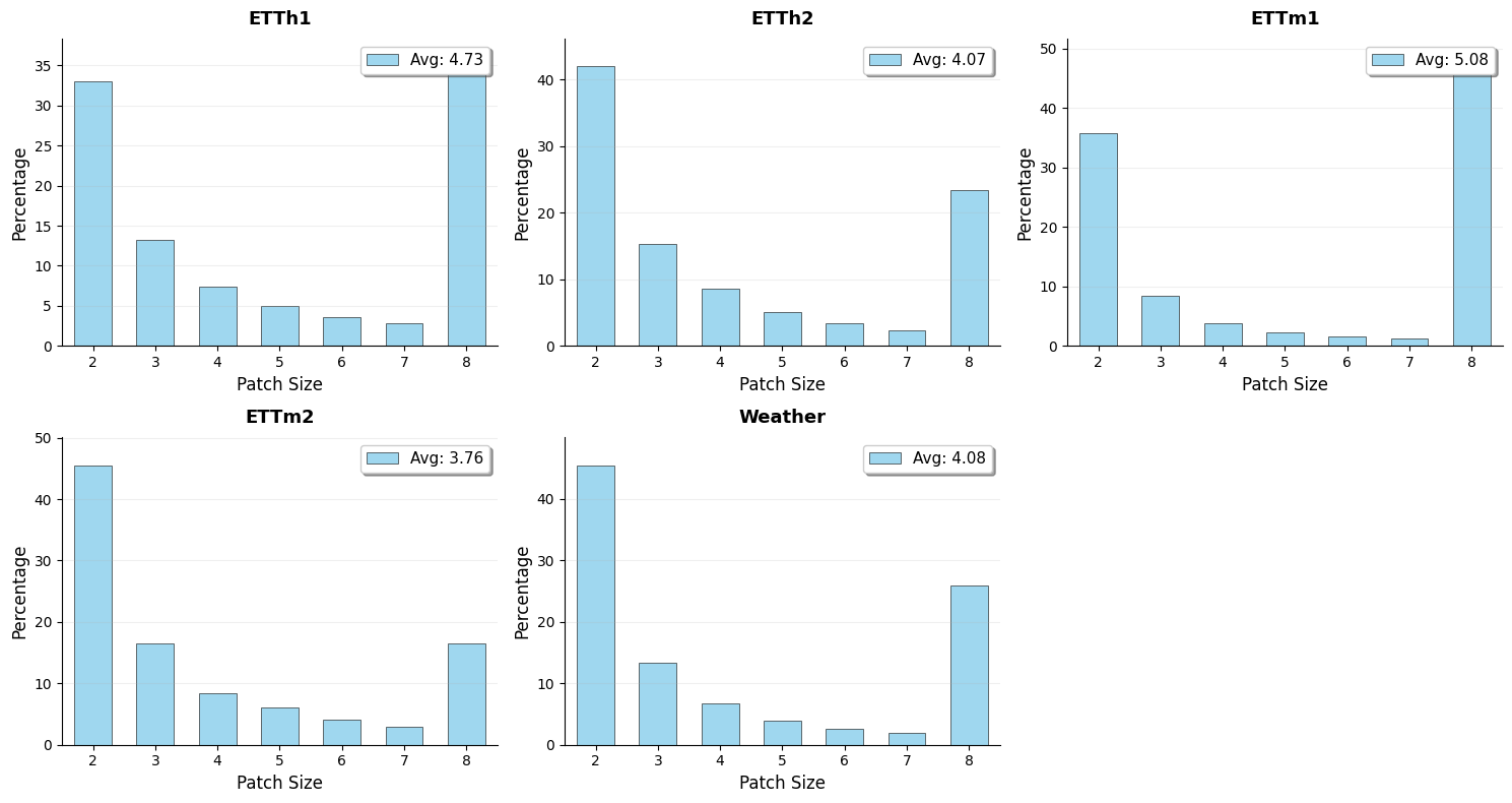
Appendix J Patch distribution

We provide the visualization of patch size distributions for each of the eval datasets in Figures 11. As we can see, weather dataset has slower variation in data resulting in larger avg patch size, whereas ETTm2 data has several regions with rapidly varying signal, resulting in much smaller patch sizes.

Figure 11: Distribution of patch sizes across eval datasets.

Appendix K Visualization of forecasts

We provide the visualization of forecasting results for an example segment of 128 samples from each of the evaluation datasets in Figures 12, 13, and 14. As observed, the Weather dataset exhibits relatively smooth and slowly varying dynamics, making forecasts easier to capture, whereas the ETTm datasets contain regions with rapid fluctuations, which pose greater challenges for accurate prediction.

(a) ETTh1

(b) ETTh2

Figure 12: Forecasting results on ETTh1 and ETTh2 datasets.

(a) ETTm1

(b) ETTm2

Figure 13: Forecasting results on ETTm1 and ETTm2 datasets.

(a) Weather

Figure 14: Forecasting results on the Weather dataset.