Identifying the Group to Intervene on to Maximise Effect Under Cross-Group Interference

Abstract.

In many networked systems, interventions applied to one group of units can induce substantial causal effects on another group through cross-group interference pathways. Despite its practical importance in domains such as public health, digital marketing, and social policy, the problem of identifying which intervention subset in a source group maximizes the benefit on a target group remains largely unaddressed. We formalize this problem as cross-group causal influence estimation and introduce the core-to-group causal effect (Co2G), a formally defined causal estimand that quantifies the contrast in target-group outcomes under intervention versus non-intervention on a candidate source subset. We establish the nonparametric identifiability of Co2G from observational network data using do-calculus under standard causal assumptions, and develop a graph neural network–based estimator that captures cross-group interference patterns. To navigate the combinatorial search space of candidate subsets, we propose CauMax, an uncertainty-aware causal effect maximization framework with two scalable selection algorithms: (i) CauMax-G, an iterative greedy search with Monte Carlo dropout–based lower confidence bounds, and (ii) CauMax-D, a differentiable gradient-based optimization via Gumbel–Softmax relaxation. Extensive experiments on two real-world social networks demonstrate that CauMax achieves an order-of-magnitude reduction in regret compared with structural heuristics and diffusion-based baselines, and that moderate uncertainty penalization consistently improves subset selection quality.

1. Introduction

In many real-world systems, interventions applied to one group of entities can induce substantial causal effects on other distinct groups through complex interaction structures. Such phenomena arise broadly in social (Yang et al., 2024), economic (Han et al., 2023), biological (Ma et al., 2023), and online systems (Yuan et al., 2021), where individuals or units are embedded in networks that mediate indirect effects across group boundaries. In these settings, an intervention targeting a subset of units may influence outcomes of other units that are not directly treated, giving rise to interference and violating the standard assumption that each unit’s outcome depends only on its own treatment assignment. Understanding and quantifying causal effects under interference has therefore become a central challenge in modern causal inference on networked data (Imai et al., 2021; Imbens and Rubin, 2015; Ogburn et al., 2024).

A schematic diagram showing two groups of nodes, Group A (source) and Group B (target). Group A displays a complex network structure with interconnected nodes, where four nodes are highlighted in red as an intervention subset. An arrow labeled ’Cross-group causal interference’ points from Group A to Group B. Group B is enclosed in a dashed box and also shows an internal network structure.

Figure 1. Illustration of the cross-group causal interference problem. The source group $A$ forms a complex interaction structure, and an intervention can be applied to any candidate subset. The goal is to identify the subset that creates the maximal effect on target group $B$. The causal mechanism operates through cross-group interference pathways from $A$ to $B$. For a subset, the counterfactual perspective compares the target group-level outcomes under intervention and non-intervention on a subset. Red nodes denote a candidate intervention subset.

One prominent motivating domain where cross-group causal interference plays a crucial role is epidemiology. Epidemiological studies have long shown that the role of core transmitters in the spread of infectious diseases far exceeds their proportion in the population (Anderson and May, 1991; Boily et al., 2002). Although core groups, such as highly connected individuals or central clusters in epidemiological networks, represent only a small fraction of the population, their high contact rates and concentrated interactions make them the dominant sources of transmission. Consequently, disease spread is highly heterogeneous rather than uniform across populations, and interventions targeting highly connected regions can induce spillover effects that propagate widely through social contact networks (Schieber et al., 2023; Cui and Zhu, 2024). These findings highlight a fundamental methodological challenge: under network interference, how can we formally identify which core groups generate the largest causal influence, particularly when their own group produces cross-group spillovers? Understanding such cross-group causal influence is crucial for designing targeted interventions in real-world systems where social, behavioral, or biological interactions routinely span community boundaries.

Motivating Example 1. Public vaccination programs offer a compelling illustration of how interventions targeted at one population segment can generate substantial causal effects on another. In many regions, elderly individuals or patients with severe chronic conditions cannot be directly vaccinated, making their protection dependent on interventions targeting other core sources of transmission, such as highly connected working-age adults or densely interacting social groups. Vaccinating a particular core subgroup reduces its members’ infection risk and, crucially, lowers disease transmission to elderly communities that remain unvaccinated. Different choices of core groups lead to markedly different target benefits, as each subgroup interacts with the elderly through distinct contact patterns and transmission pathways. These indirect protective effects constitute a form of cross-group causal influence, as illustrated in Figure 1. The key challenge is that observed infection outcomes among the elderly reflect only the intervention actually implemented, whereas policy decisions require understanding how these outcomes would have differed under alternative intervention choices and identifying the one that maximizes the causal benefit on the target.

Motivating Example 2. Digital product ecosystems often exhibit cross-group influence, where interventions applied to one community reshape the behavior of another. Consider a company launching a new AI-powered note-taking application and seeking to increase adoption among students. Because direct intervention on students is limited, the company instead provides a free premium version to selected online content creators. Treating these creators increases their own usage and encourages them to feature the product in their content, indirectly exposing the target student community and raising adoption without direct intervention. Importantly, creators differ substantially in their target impact: only a small subset may strongly influence students’ adoption decisions. However, the company observes outcomes only under the intervention applied to a given set of creators. Effective decision making therefore requires understanding how student adoption would have differed had the intervention targeted alternative creator subsets, a fundamentally counterfactual question involving cross-group causal influence.

Table 1. Representative works related to network interference and influence.

Representative Works	Cross-Group	Causal Effect Max.
Jiang and Sun (2022)	✗	✗
Cai et al. (2023)	✗	✗
Aronow and Samii (2017)	✗	✗
Ogburn et al. (2024)	✗	✗
Miguel and Kremer (2004)	✓	✗
Heitzig and O’Keeffe-O’Donovan (2024)	✓	✗
Ji et al. (2025)	✓	✗
Possnig et al. (2022)	✗	✗
Lee et al. (2023)	✗	✗
Su et al. (2025)	✗	✓
Ours	✓	✓

These intertwined diffusion mechanisms highlight the limitations of existing causal inference frameworks under network interference. As summarized in Table 1, most previous studies either confine spillovers within a single community (Jiang and Sun, 2022; Cai et al., 2023; Aronow and Samii, 2017; Ogburn et al., 2024) or fail to capture the asymmetric influence exerted by highly active core groups (Miguel and Kremer, 2004; Heitzig and O’Keeffe-O’Donovan, 2024; Ji et al., 2025; Possnig et al., 2022). While recent work has begun to formalize influential individuals’ causal influence, such as Lee et al. (Lee et al., 2023) who propose a causal framework to identify influential subjects within a single network, their formulation restricts interference to occur within rather than across groups and does not characterize how interventions propagate between communities. In parallel, Su et al. (Su et al., 2025) investigate the environmental sensitivity of influence maximization gains, but their analysis is grounded in algorithmic diffusion models rather than causal estimates, and thus cannot distinguish marginal structural influence from genuine causal spillovers or capture how activation effects transmit across heterogeneous groups. Consequently, existing approaches cannot identify which core sources generate the largest cross-group causal influence, a capability essential for targeting interventions in realistic settings where communities interact, overlap, and exert asymmetric effects on one another.

While classical greedy influence-maximization (IM) methods aim to select seeds that maximize the expected cascade size under a pre-specified diffusion model (Kempe et al., 2003; Chen et al., 2009), this perspective fundamentally differs from our objective. Greedy IM algorithms simulate how activation spreads under assumed diffusion dynamics, whereas we seek to determine how outcomes in group B would change under different choices of core sources to target in group A. This distinction is crucial: even perfectly predicting the observed diffusion cannot reveal how group B would have responded had an alternative subset in group A been selected, because such responses correspond to potential outcomes that are never observed in real data (Rubin, 2005; Imbens and Rubin, 2015). Therefore, identifying the core source that maximizes cross-group improvements requires a causal formulation rather than a purely diffusion-based or algorithmic one. A causal perspective explicitly defines the estimand of interest, clarifies what is identifiable from observational data, and enables principled comparison across intervention choices that were not carried out.

However, identifying which source subset yields the greatest target improvement poses two fundamental challenges. (a) Unbiased estimation under cross-group interference. Because treatments assigned to units in a subset in the source network $A$ spill over to units in $B$ through complex network pathways, the potential outcomes corresponding to alternative subsets cannot be observed simultaneously. Standard estimators conflate causal spillovers with correlations induced by network structure or confounding, making the underlying causal contrast difficult to identify from observational data. (b) The combinatorial search space of intervention choices. The number of possible subsets grows exponentially with $|A|$, rendering exhaustive evaluation of all counterfactual outcomes infeasible. Classical influence-maximization heuristics are not directly applicable, as they optimize expected cascade sizes under assumed diffusion models rather than causal estimands defined over unobserved potential outcomes. Together, these challenges motivate the need for a framework that (i) identifies unbiased cross-group causal effects from observational network data and (ii) efficiently discovers the subset that maximizes target improvement.

Motivated by these observations, we formulate the problem of cross-group causal influence maximization, which seeks to identify the core sources whose selection for intervention yields the greatest causal improvements in the outcomes of other groups. Our main contributions are summarized as follows:

• Problem formulation. We formalize the problem of cross-group causal influence maximization and define the core-to-group causal effect (Co2G), a causal estimand that quantifies the target-group outcome improvement attributable to intervening on a source subset under network interference.

• Nonparametric identifiability. We establish the identifiability of Co2G from observational network data using do-calculus under standard graphical causal assumptions, without imposing parametric restrictions on the outcome model.

• Estimation and optimization framework. We propose CauMax, a causal effect maximization framework that integrates a graph neural network-based estimator for cross-group interference with an uncertainty-aware optimization objective based on Monte Carlo dropout. We instantiate two scalable subset selection algorithms: CauMax-G, an iterative greedy search, and CauMax-D, a differentiable gradient-based method via Gumbel–Softmax relaxation.

• Empirical evaluation. Extensive experiments on BlogCatalog and Flickr demonstrate that the proposed framework achieves an order-of-magnitude reduction in regret over structural and diffusion-based baselines, and that moderate uncertainty penalization consistently improves selection quality.

It shows a source group V_A with overlapping communities and a target group V_B.

Figure 2. Cross-group causal structure and network-to-causal abstraction. (a) Network representation conditioned on a candidate subset $S\subseteq V_{A}$, with source units partitioned into the intervened subset $S$ and remaining units $V_{A}\setminus S$. (b) The core-to-group causal effect (Co2G), contrasting the target group outcome $Y_{B}$ under intervention versus non-intervention on $S$. (c) Corresponding causal graph with subset-level variables: $X_{S},X_{V_{A}\setminus S},X_{V_{B}}$ (pre-treatment covariates), $T_{S},T_{V_{A}\setminus S}$ (treatment assignments), and $Y_{B}$ (target outcomes).

2. Related Work

Our work lies at the intersection of causal inference under network interference and influence maximization on social networks. We review each line of work below.

2.1. Cross-Group Spillovers in Networked Systems

Classical causal inference under interference has primarily operated under the partial interference assumption (Hudgens and Halloran, 2008; Sobel, 2006), where spillovers occur only within pre-defined clusters. Extensions to networked observational data (Aronow and Samii, 2017; Forastiere et al., 2021; Ogburn et al., 2024) allow more flexible interference structures but remain confined to within-group or neighborhood-level effects.

More recent work has examined spillovers that propagate across distinct communities. Miguel and Kremer (2004) provided early empirical evidence of cross-school treatment externalities in deworming programs. Heitzig and O’Keeffe-O’Donovan (2024) documented cross-village diffusion of savings groups, and Ji et al. (2025) revealed heterogeneous within- and cross-group spillover effects in influencer marketing. On the estimation side, Jiang and Sun (2022) and Cai et al. (2023) developed representation learning-based estimators and generalization bounds for causal effects on networked data, though their formulations do not explicitly distinguish source and target groups or model asymmetric cross-group interference. In contrast, our framework formalizes a directional cross-group causal structure where interventions on a source group propagate to a target group through inter-group network connections, and introduces a combinatorial optimization objective over causal estimands.

2.2. Influence Maximization

Influence maximization (IM) selects seed nodes to maximize expected cascade spread under diffusion models such as IC and LT (Kempe et al., 2003; Chen et al., 2009; Leskovec et al., 2007). Recent work has begun to connect IM with causal reasoning: Lee et al. (2023) proposed a causal framework for identifying influential subjects within a single network, while Su et al. (2025) incorporated individual treatment effects into IM to capture environmental sensitivity of node-level gains.

However, IM fundamentally differs from our objective. IM algorithms optimize expected activation counts under assumed diffusion dynamics, whereas we optimize a formally defined causal estimand the core-to-group causal effect (Co2G) over unobserved potential outcomes. Even perfect diffusion prediction cannot reveal how the target group would have responded under alternative intervention subsets, as these correspond to counterfactual outcomes never observed in data (Imbens and Rubin, 2015; Rubin, 2005). Our framework bridges this gap by combining causal identification with subset optimization over estimated causal effects.

3. Problem Setup and Cross-Group Interference

Notation.

Let $V_{A}$ denote the set of source-group nodes and $V_{B}$ denote the set of target-group nodes. A (candidate) intervention subset is denoted by $S\subseteq V_{A}$ with a budget constraint $|S|\leq K$. We use $\mathcal{S}$ to denote a collection of evaluated subsets (e.g., randomly sampled subsets of varying sizes) in empirical evaluation. For a fixed size $k$, let $S_{k}$ denote the subset returned by an algorithm, and let $S_{k}^{\star}$ denote the oracle optimal subset under the ground-truth causal effect.

Networked Groups and Interference Structure.

We consider two disjoint groups of units: a source group and a target group, corresponding to node sets $V_{A}$ and $V_{B}$, respectively. Edges may exist both within groups and across groups, forming an interaction graph through which influences originating in the source group may propagate to the target group via direct or indirect pathways. The interference pattern is asymmetric: interventions applied to units in group $A$ may affect outcomes in group $B$, but not vice versa. Such directional cross-group influence patterns arise naturally in many real-world settings, including vaccination and infectious disease control (Miguel and Kremer, 2004; Jiang and Sun, 2022), influencer marketing and information diffusion (Lee et al., 2023; Ji et al., 2025), and core–periphery or hierarchical social systems (Kempe et al., 2003; Schieber et al., 2023).

Subset-Level Intervention.

We focus on deterministic joint interventions applied to a subset $S\subseteq V_{A}$. All units in $S$ are simultaneously assigned to the same treatment level, while units in $V_{A}\setminus S$ are fixed at a baseline (control) level. Throughout the paper, we assume a binary treatment with levels $t\in\{0,1\}$ and fix the baseline level as $t_{0}=0$. Our objective is to identify, among a combinatorial space of candidate subsets $S\subseteq V_{A}$, the subset-level intervention that maximizes the causal effect on the target group $B$.

Interventional Target-Group Mean.

Let $Y_{j}$ denote the outcome of target node $j\in V_{B}$, and define the average target-group outcome as $Y_{B}=\frac{1}{|V_{B}|}\sum_{j\in V_{B}}Y_{j}.$ For any subset $S\subseteq V_{A}$ and treatment level $t\in\{0,1\}$, we define the interventional target-group mean as

(1) $$\mu_{B}(t;S)\;:=\;\mathbb{E}\!\left[Y_{B}\;\middle|\;\mathrm{do}(T_{S}=t),\,\mathrm{do}(T_{V_{A}\setminus S}=t_{0})\right],$$

where $t_{0}=0$ denotes the baseline intervention level for the remaining source nodes.

Core-to-Group Causal Effect.

The core-to-group causal effect (Co2G) of subset $S$ is defined as the contrast between two interventional target-group means:

(2) $$\mathrm{Co2G}(S)\;:=\;\mu_{B}(1;S)-\mu_{B}(0;S).$$

Cross-Group Causal Influence Maximization.

Given an intervention budget $K$, the cross-group causal influence maximization problem seeks to identify

(3) $$S^{\star}\;=\;\arg\max_{S\subseteq V_{A},\;|S|\leq K}\mathrm{Co2G}(S),$$

that is, to select at most $K$ source nodes whose joint intervention yields the largest causal improvement in the outcomes of the target group $B$.

We state the standard assumptions commonly adopted in causal inference to support the identification results presented in the subsequent sections.

Assumption 3.1 (Markov Property (Pearl, 2009)).

Let $\mathcal{G}$ denote the directed acyclic graph (DAG) corresponding to the causal abstraction in Fig. 2. The joint distribution over the observed variables satisfies the Markov property with respect to $\mathcal{G}$, i.e., each variable is independent of its non-descendants given its parents in $\mathcal{G}$.

Assumption 3.2 (Faithfulness (Spirtes et al., 2000)).

The observed data distribution is faithful to the causal graph $\mathcal{G}$, meaning that all and only the conditional independence relationships implied by $\mathcal{G}$ hold in the distribution.

Assumption 3.3 (Causal Sufficiency (Pearl, 2009)).

All common causes of the observed variables in the causal graph $\mathcal{G}$ are observed. In particular, there are no unobserved confounders jointly affecting the treatment assignments in $V_{A}$ and the target outcomes in $V_{B}$ after conditioning on observed covariates.

Assumption 3.4 (Positivity (Pearl, 2009)).

For any subset $S\subseteq V_{A}$ with $|S|\leq K$, any treatment level $t\in\{0,1\}$, and any covariate realization $x$ with $p(X=x)>0$, we assume $\Pr\!\big(T_{S}=t,\;T_{V_{A}\setminus S}=t_{0}\mid X=x\big)>0,$ where $t_{0}=0$ denotes the baseline intervention level.

4. Method

In this section, we present the full framework for cross-group causal effect estimation and optimization. We first establish the nonparametric identifiability of the Co2G from observational data (Section 4.1), then develop a learning-based estimator and optimization procedure consisting of three components: (1) a graph neural network estimator that captures cross-group interference patterns (Section 4.2), (2) an uncertainty-aware optimization objective that guards against out-of-distribution predictions (Section 4.3), and (3) two scalable search algorithms for subset selection (Section 4.4).

4.1. Identifiability of the Cross-Group Causal Effect

We now establish the identifiability of the interventional target-group mean $\mu_{B}(t;S)$ and the corresponding core-to-group causal effect $\mathrm{Co2G}(S)$ defined in Eqs. (1)–(2) under the cross-group causal structure illustrated in Fig. 2. Let $X=\big(X_{V_{A}},\;X_{V_{B}}\big)$ denote the collection of observed pre-treatment covariates, where $X_{V_{A}}$ denotes covariates of source-group nodes, and $X_{V_{B}}$ denotes covariates of target-group nodes. By construction, all variables in $X$ are measured prior to treatment assignment and are not affected by any intervention.

Our goal is to identify, from observational data, the interventional mean $\mu_{B}(t;S)=\mathbb{E}\!\left[Y_{B}\;\middle|\;\mathrm{do}(T_{S}=t),\,\mathrm{do}(T_{V_{A}\setminus S}=t_{0})\right],$ for any subset $S\subseteq V_{A}$ with $|S|\leq K$ and treatment level $t\in\{0,1\}$, where $t_{0}=0$ denotes the baseline intervention level.

Theorem 4.1 (Identifiability of the Interventional Target-Group Mean).

Under Assumptions 3.1 to 3.4 and the causal graph in Fig. 2, the interventional target-group mean $\mu_{B}(t;S)$ is identifiable from the observational distribution $p(X,T_{V_{A}},Y_{B})$ and admits the following representation:

(4) $$\mu_{B}(t;S)=\sum_{x}\mathbb{E}\!\left[Y_{B}\mid T_{S}=t,\;T_{V_{A}\setminus S}=t_{0},\;X=x\right]\,p(X=x).$$

Proof.

Starting from the definition of the interventional distribution, $P(y_{B}\mid\mathrm{do}(T_{S}=t),\mathrm{do}(T_{V_{A}\setminus S}=t_{0}))$. By the law of total probability, we have $P(y_{B}\mid\mathrm{do}(T_{S}=t),\mathrm{do}(T_{V_{A}\setminus S}=t_{0}))=\sum_{x}P(y_{B}\mid X=x,\mathrm{do}(T_{S}=t),\mathrm{do}(T_{V_{A}\setminus S}=t_{0}))\times P(X=x\mid\mathrm{do}(T_{S}=t),\mathrm{do}(T_{V_{A}\setminus S}=t_{0}))$. Based on Rule 3 of do-calculus, we have $P(X=x\mid\mathrm{do}(T_{S}=t),\mathrm{do}(T_{V_{A}\setminus S}=t_{0}))=P(X=x\mid\mathrm{do}(T_{S}=t))$, since $X\perp\!\!\!\perp T_{V_{A}\setminus S}\mid T_{S}$ in $\mathcal{G}_{\overline{T_{S}},\,\overline{T_{V_{A}\setminus S}}}$, where $\overline{T}$ denotes the removal of all incoming edges into $T$. Applying Rule 3 again yields $P(X=x\mid\mathrm{do}(T_{S}=t))=P(X=x)$, because $X\perp\!\!\!\perp T_{S}$ in $\mathcal{G}_{\overline{T_{S}}}$.

Next, by Rule 2 of do-calculus, we have $P(y_{B}\mid X=x,\mathrm{do}(T_{S}=t),\mathrm{do}(T_{V_{A}\setminus S}=t_{0}))=P(y_{B}\mid X=x,\mathrm{do}(T_{S}=t),T_{V_{A}\setminus S}=t_{0})$ because $Y_{B}\perp\!\!\!\perp T_{V_{A}\setminus S}\mid(T_{S},X)$ in $\mathcal{G}_{\overline{T_{S}},\,\underline{T_{V_{A}\setminus S}}}$, where $\underline{T}$ denotes the removal of all outgoing edges from $T$. Similarly, $P(y_{B}\mid X=x,\mathrm{do}(T_{S}=t),T_{V_{A}\setminus S}=t_{0})=P(y_{B}\mid X=x,T_{S}=t,T_{V_{A}\setminus S}=t_{0})$, because $Y_{B}\perp\!\!\!\perp T_{S}\mid(T_{V_{A}\setminus S},X)$ in $\mathcal{G}_{\underline{T_{S}}}$. Combining the above results, we obtain the identification formula $P(y_{B}\mid\mathrm{do}(T_{S}=t),\mathrm{do}(T_{V_{A}\setminus S}=t_{0}))=\sum_{x}P(y_{B}\mid X=x,T_{S}=t,T_{V_{A}\setminus S}=t_{0})\,P(X=x)$. ∎

Corollary 4.2 (Identifiability of the Core-to-Group Causal Effect).

For any subset $S\subseteq V_{A}$ with $|S|\leq K$, the core-to-group causal effect $\mathrm{Co2G}(S)=\mu_{B}(1;S)-\mu_{B}(0;S)$ is identifiable and can be expressed as

(5) $$\mathrm{Co2G}(S)=\sum_{x}\Big( \mathbb{E}[Y_{B}\mid T_{S}=1,T_{V_{A}\setminus S}=t_{0},X=x]$$

$$\;-\;\mathbb{E}[Y_{B}\mid T_{S}=0,T_{V_{A}\setminus S}=t_{0},X=x]\Big)\,p(X=x).$$

4.2. Causal Effect Estimator

As established in section 4.1, the interventional target-group mean $\mu_{B}(t;S)$ and the core-to-group causal effect $\mathrm{Co2G}(S)$ are identifiable from observational data under Assumptions 3.1 to 3.4. We now introduce a parameterized estimator designed to approximate these identified causal quantities from networked observational data.

Estimator Overview.

Let $f_{\theta}$ denote a learned causal effect estimator. Given a subset $S\subseteq V_{A}$ and a treatment level $t\in\{0,1\}$, we represent the corresponding joint intervention $\mathrm{do}(T_{S}=t,\,T_{V_{A}\setminus S}=t_{0})$ by a binary treatment vector $T(S,t)\in\{0,1\}^{|V_{A}|}$, where

(6) $$T_{i}(S,t)=\begin{cases}t,&i\in S,\\ t_{0},&i\in V_{A}\setminus S,\end{cases}\qquad t_{0}=0.$$

The estimator $f_{\theta}$ takes as input the network structure, node covariates, and the subset-induced treatment vector $T(S,t)$, and outputs a prediction of the corresponding interventional target-group mean:

(7) $$\widehat{\mu}_{B}(t;S)=f_{\theta}\!\big(T(S,t)\big).$$

The estimated core-to-group causal effect is then given by

(8) $$\widehat{\mathrm{Co2G}}(S)=\widehat{\mu}_{B}(1;S)-\widehat{\mu}_{B}(0;S).$$

Model Architecture.

The estimator $f_{\theta}$ is implemented as a graph-based neural architecture that explicitly models how subset-level interventions on the source group propagate to outcomes in the target group. The architecture consists of three components. (i) Source-group encoder. For each source node $i\in V_{A}$, we construct an input representation by concatenating its observed covariates $X_{i}$ with the subset-induced treatment indicator $T_{i}(S,t)$. A graph neural network (GNN) (Wu et al., 2020) is then applied to the induced subgraph of $V_{A}$ to produce context-aware node embeddings that capture both within-group dependencies and the direct effect of the intervention. (ii) Cross-group interference aggregation. To model cross-group spillovers, we propagate information from source nodes to target nodes along cross-group edges. For each target node $j\in V_{B}$, we aggregate the representations of its source-group neighbors in $V_{A}$ along cross-group edges. Specifically, let $N_{A}(j)=\{i\in V_{A}:(i,j)\in E_{AB}\}$ denote the set of source nodes connected to $j$. A permutation-invariant aggregation operator is applied over $\{h_{i}:i\in N_{A}(j)\}$ to produce an interference representation $m_{j}$, which summarizes the spillover effect from the source group to node $j$. In our implementation, we use mean pooling for aggregation, i.e., $m_{j}=\frac{1}{|N_{A}(j)|}\sum_{i\in N_{A}(j)}h_{i}$. (iii) Target outcome prediction. The aggregated interference signal is combined with the covariates of target node $j$ and passed through a prediction network to obtain a predicted outcome $\widehat{Y}_{j}(t;S)$. The estimated interventional target-group mean is then computed as

(9) $$\widehat{\mu}_{B}(t;S)=\frac{1}{|V_{B}|}\sum_{j\in V_{B}}\widehat{Y}_{j}(t;S),$$

which serves as the model-based approximation of $\mu_{B}(t;S)$.

4.3. Uncertainty-Aware Optimization Objective

Given the estimator $\widehat{\mathrm{Co2G}}(S)$, a natural approach would be to select the subset $S$ that maximizes the predicted causal effect. However, since $f_{\theta}$ is learned from finite observational data, predictions for subsets that are far from the support of the observed data may suffer from high epistemic uncertainty.

To account for this uncertainty, we adopt a risk-averse optimization criterion based on a lower confidence bound (LCB). For a candidate subset $S\subseteq V_{A}$, we perform $M$ stochastic forward passes using Monte Carlo dropout (Gal and Ghahramani, 2016) and obtain samples $\{\widehat{\mathrm{Co2G}}^{(m)}(S)\}_{m=1}^{M}$. We compute the empirical mean and standard deviation as follows:

(10) $$\widehat{\mu}_{\mathrm{Co2G}}(S) =\frac{1}{M}\sum_{m=1}^{M}\widehat{\mathrm{Co2G}}^{(m)}(S),$$

(11) $$\widehat{\sigma}_{\mathrm{Co2G}}(S) =\sqrt{\frac{1}{M}\sum_{m=1}^{M}\left(\widehat{\mathrm{Co2G}}^{(m)}(S)-\widehat{\mu}_{\mathrm{Co2G}}(S)\right)^{2}}.$$

The uncertainty-aware objective is defined as

(12) $$J(S)=\widehat{\mu}_{\mathrm{Co2G}}(S)-\lambda\,\widehat{\sigma}_{\mathrm{Co2G}}(S),$$

where $\lambda\geq 0$ controls the strength of uncertainty penalization. Maximizing $J(S)$ favors subsets with large predicted causal effects while discouraging selections associated with high uncertainty.

4.4. Subset Selection Algorithms

Greedy Search.

For small to medium-sized networks, we adopt an iterative greedy procedure to approximately solve $\max_{S\subseteq V_{A}}J(S)$ subject to $|S|\leq K$. Starting from the empty set $S_{0}=\emptyset$, at iteration $k$ we select the node that yields the largest marginal improvement in the uncertainty-aware objective:

(13) $$v^{\star}=\arg\max_{v\in V_{A}\setminus S_{k-1}}\big[J(S_{k-1}\cup\{v\})-J(S_{k-1})\big].$$

If the maximum marginal gain is positive, we update $S_{k}=S_{k-1}\cup\{v^{\star}\}$; otherwise, the procedure terminates early. The algorithm stops once $|S_{k}|=K$ or no further improvement is possible. The full procedure is summarized in Algorithm 1.

Differentiable Subset Optimization.

For large-scale source groups, the greedy procedure in Algorithm 1 becomes computationally expensive due to repeated evaluations of $J(S)$. To address this limitation, we introduce a differentiable relaxation that enables gradient-based optimization of the same uncertainty-aware objective.

Instead of directly optimizing over discrete subsets, we relax the subset indicator to a continuous vector and optimize a smooth surrogate of $J(S)$ while enforcing the budget constraint. After optimization, a discrete subset is recovered via a top-$K$ projection. The resulting procedure is summarized in Algorithm 2.

Each source node $i\in V_{A}$ is associated with a learnable logit $\psi_{i}$. A relaxed treatment vector $\widetilde{T}\in[0,1]^{|V_{A}|}$ is generated via a Gumbel–Softmax reparameterization (Jang et al., 2017), which can be interpreted as a soft approximation of a subset-induced intervention. The estimator $f_{\theta}$ is kept fixed, and the logits $\psi$ are optimized to maximize the uncertainty-aware objective under a budget constraint:

(14) $$\min_{\psi}\;-\mathbb{E}_{g\sim\text{Gumbel}}[J(\tilde{T}(\psi,g))]+\gamma\left(\|\tilde{T}(\psi,g)\|_{1}-K\right)^{2},$$

where $\tilde{T}(\psi,g)=\sigma((\psi+g)/\tau)$ is the Gumbel–Softmax relaxation and the expectation is taken over the Gumbel noise $g$. After optimization, a discrete subset $S$ is obtained by selecting the top-$K$ nodes according to $\psi$. This approach scales linearly with $|V_{A}|$ and is suitable for large-scale networks.

Algorithm 1 Uncertainty-Aware Greedy Search (CauMax-G)

1:Trained estimator $f_{\theta}$; source nodes $V_{A}$; budget $K$; MC passes $M$; uncertainty penalty $\lambda$

2:Selected subset $S$

3:$S\leftarrow\emptyset$

4:Estimate $J(S)=\widehat{\mu}_{\mathrm{Co2G}}(S)-\lambda\,\widehat{\sigma}_{\mathrm{Co2G}}(S)$ using $M$ MC-dropout passes

5:for $k=1$ to $K$ do

6:  $\Delta^{\star}\leftarrow-\infty$, $v^{\star}\leftarrow\text{None}$

7:  for all $v\in V_{A}\setminus S$ do

8:   Estimate $J(S\cup\{v\})$ using $M$ MC-dropout passes

9:   $\Delta\leftarrow J(S\cup\{v\})-J(S)$

10:   if $\Delta>\Delta^{\star}$ then

11:     $\Delta^{\star}\leftarrow\Delta$

12:     $v^{\star}\leftarrow v$

13:   end if

14:  end for

15:  if $\Delta^{\star}>0$ then

16:   $S\leftarrow S\cup\{v^{\star}\}$

17:   Update cached $J(S)$

18:  else

19:   break

20:  end if

21:end for

22:return $S$

Algorithm 2 Differentiable Gradient Search (CauMax-D)

1:Effect estimator $f_{\theta}$; source nodes $V_{A}$; budget $K$; iterations $M_{\mathrm{iter}}$; learning rate $\eta$; MC passes $M$; uncertainty penalty $\lambda$; regularization $\gamma$

2:Selected subset $S_{K}$

3:Initialize $\psi\sim\mathcal{N}(0,0.01I)$

4:for $m=1$ to $M_{\mathrm{iter}}$ do

5:  Sample $g\sim\mathrm{Gumbel}(0,1)^{|V_{A}|}$

6:  Generate soft mask $\widetilde{T}\leftarrow\sigma\!\left((\psi+g)/\tau\right)$ $\triangleright$ $\widetilde{T}\in[0,1]^{|V_{A}|}$ is a continuous relaxation of the subset indicator

7:  Estimate $\widehat{\mu}_{\mathrm{Co2G}}(\widetilde{T})$ and $\widehat{\sigma}_{\mathrm{Co2G}}(\widetilde{T})$ using $M$ MC-dropout passes

8:  $J(\widetilde{T})\leftarrow\widehat{\mu}_{\mathrm{Co2G}}(\widetilde{T})-\lambda\,\widehat{\sigma}_{\mathrm{Co2G}}(\widetilde{T})$

9:  $\mathcal{L}\leftarrow-J(\widetilde{T})+\gamma\left(\|\widetilde{T}\|_{1}-K\right)^{2}$

10:  $\psi\leftarrow\psi-\eta\nabla_{\psi}\mathcal{L}$

11:end for

12:$S_{K}\leftarrow\textsc{TopK\_Indices}(\psi,K)$

13:return $S_{K}$

5. Experiments

We evaluate the proposed framework on two real-world social networks, BlogCatalog (BC) and Flickr. Our experiments address three questions: (i) whether the proposed estimator accurately recovers cross-group causal effects, (ii) whether uncertainty-aware selection reduces regret over heuristic baselines, and (iii) how the two optimization strategies compare across network sizes.

5.1. Baselines

We compare against: Random, which selects $K$ source nodes uniformly at random (Kempe et al., 2003); Degree, which selects the $K$ highest-degree source nodes (Kenett et al., 2015); and Influence Maximization (IM), which selects nodes to maximize diffusion-based cascade spread without considering causal effects (Leskovec et al., 2007). We evaluate two variants of CauMax: CauMax-G (Algorithm 1), an iterative greedy search, and CauMax-D (Algorithm 2), a differentiable gradient-based method with Top-$K$ projection.

5.2. Evaluation Metrics

Approximate Oracle Subset ($S_{k}^{\star}$).

To assess the quality of a selected subset, we construct an approximate oracle solution using access to the ground-truth causal effect. For a fixed budget $k$, the oracle subset is defined as $S_{k}^{\star}=\arg\max_{S\subseteq V_{A},\;|S|=k}\mathrm{Co2G}(S),$ where $\mathrm{Co2G}(S)$ denotes the true core-to-group causal effect computed from the data-generating process. Since exhaustive enumeration over all $\binom{|V_{A}|}{k}$ subsets is computationally infeasible, we approximate $S_{k}^{\star}$ using a greedy procedure that incrementally adds the source node with the largest marginal increase in the true $\mathrm{Co2G}(\cdot)$. This procedure, referred to as Oracle-Greedy, serves as a computationally tractable proxy for the true oracle and is used only for evaluation purposes.

Regret@k.

Given a method that returns a subset $S_{k}$ of size $k$, we define the regret as $\mathrm{Regret@}k=\mathrm{Co2G}(S_{k}^{\star})-\mathrm{Co2G}(S_{k}),$ which measures the performance gap between the selected subset and the approximate oracle. Lower regret indicates that the selected subset achieves a causal effect closer to the oracle solution.

Estimation Error.

In addition to subset-level performance, we evaluate the accuracy of the causal effect estimator by computing the root mean squared error (RMSE) between the estimated and true core-to-group causal effects over a collection of evaluated subsets $\mathcal{S}$: $\mathrm{RMSE}=\sqrt{\frac{1}{|\mathcal{S}|}\sum_{S\in\mathcal{S}}\big(\widehat{\mathrm{Co2G}}(S)-\mathrm{Co2G}(S)\big)^{2}}.$

Table 2. Comparison of Regret@$K$ and RMSE across methods on BC and Flickr ($\lambda=0.5$ for CauMax-D and CauMax-G). Bold indicates the best result; underline indicates the second best.

		Regret@$K$ $(\downarrow)$						RMSE $(\downarrow)$
Method	Dataset	$k$=5	$k$=10	$k$=15	$k$=20	$k$=30	$k$=50	$k$=5	$k$=10	$k$=15	$k$=20	$k$=30	$k$=50
CauMax-D	BC	0.0011	0.0015	0.0034	0.0030	0.0046	0.0069	0.0047	0.0059	0.0057	0.0058	0.0071	0.0081
	Flickr	0.0011	0.0021	0.0025	0.0031	0.0050	0.0065	0.0046	0.0050	0.0050	0.0057	0.0064	0.0075
CauMax-G	BC	0.0051	0.0087	0.0118	0.0147	0.0195	0.0301	0.0058	0.0054	0.0062	0.0073	0.0085	0.0103
	Flickr	0.0043	0.0079	0.0106	0.0127	0.0184	0.0278	0.0061	0.0060	0.0058	0.0070	0.0072	0.0097
Degree	BC	0.0111	0.0204	0.0280	0.0338	0.0483	0.0657	0.0096	0.0102	0.0104	0.0115	0.0132	0.0169
	Flickr	0.0101	0.0158	0.0235	0.0265	0.0415	0.0588	0.0097	0.0094	0.0110	0.0114	0.0130	0.0163
IM	BC	0.0201	0.0341	0.0427	0.0576	0.0799	0.1218	0.0137	0.0134	0.0157	0.0163	0.0181	0.0229
	Flickr	0.0162	0.0293	0.0388	0.0474	0.0732	0.0999	0.0126	0.0132	0.0141	0.0151	0.0175	0.0215
Random	BC	0.0274	0.0449	0.0646	0.0783	0.1130	0.1622	0.0189	0.0200	0.0199	0.0216	0.0246	0.0301
	Flickr	0.0228	0.0378	0.0558	0.0711	0.0941	0.1373	0.0172	0.0189	0.0194	0.0218	0.0228	0.0300

Two stacked bar charts showing the sensitivity of Regret at K to the uncertainty penalty $\lambda$. The top chart (a) displays results for the Greedy search algorithm, and the bottom chart (b) displays results for the Differentiable gradient search. The x-axis groups data by $\lambda$ values (0, 0.25, 0.5, 1.0, 2.0). Solid bars represent the BlogCatalog dataset, and hatched bars represent the Flickr dataset.

Two stacked bar charts illustrating the sensitivity of Regret@K to the uncertainty penalty $\lambda$. The top plot corresponds to CauMax-G and the bottom plot to CauMax-D. Each subplot shows six panels for budget levels $K\in\{5,10,15,20,30,50\}$, with grouped bars for $\lambda\in\{0,0.25,0.5,1.0,2.0\}$. Solid bars represent BlogCatalog and hatched bars represent Flickr.

Figure 3. Sensitivity analysis of the uncertainty penalty $\lambda$ on $\text{Regret@}K$ across both datasets and all budget levels $K\in\{5,10,15,20,30,50\}$. Solid bars represent BC and hatched bars represent Flickr.

Two stacked bar charts illustrating the sensitivity of the RMSE metric to the uncertainty penalty $\lambda$. Similar to the previous figure, the top plot corresponds to the CauMax-G search strategy, while the bottom plot corresponds to the CauMax-D search strategy. Bars compare performance on BlogCatalog and Flickr datasets across varying lambda values.

Figure 4. Sensitivity analysis of the uncertainty penalty $\lambda$ on RMSE.

5.3. Main Results

Table 2 compares all methods on BC and Flickr at $\lambda=0.5$ with the proposed methods. We make the following key observations.

The proposed methods substantially outperform all baselines.

Across all budget levels $K\in\{5,10,15,20,30,50\}$, both proposed methods achieve markedly lower regret than Degree, IM, and Random. For instance, at $K=20$ on BC, CauMax-D achieves $\text{Regret@}K=0.0030$, compared with $0.0338$ for Degree, $0.0576$ for IM, and $0.0783$ for Random, an order-of-magnitude improvement. This confirms that explicitly optimizing a causal estimand leads to more effective cross-group interventions than relying on structural heuristics or diffusion-based objectives.

CauMax-D closely tracks the oracle.

CauMax-D consistently achieves the lowest regret across both datasets and all budget levels, closely approximating the oracle-greedy solution. On Flickr, CauMax-D maintains regret at most 0.0065 even at $K=50$, whereas CauMax-G reaches 0.0278 and baselines exceed 0.05. The advantage of CauMax-D is particularly pronounced at larger budgets, where the combinatorial search space makes greedy selection more susceptible to local optima.

Estimation accuracy correlates with subset selection quality.

The RMSE results in Table 2 show a ranking broadly aligned with $\text{Regret@}K$: across most budget levels, CauMax-D achieves the lowest RMSE, followed by CauMax-G, Degree, IM, and Random. This indicates that better causal effect estimation directly translates to better subset selection.

5.4. Sensitivity to the Uncertainty Penalty $\lambda$

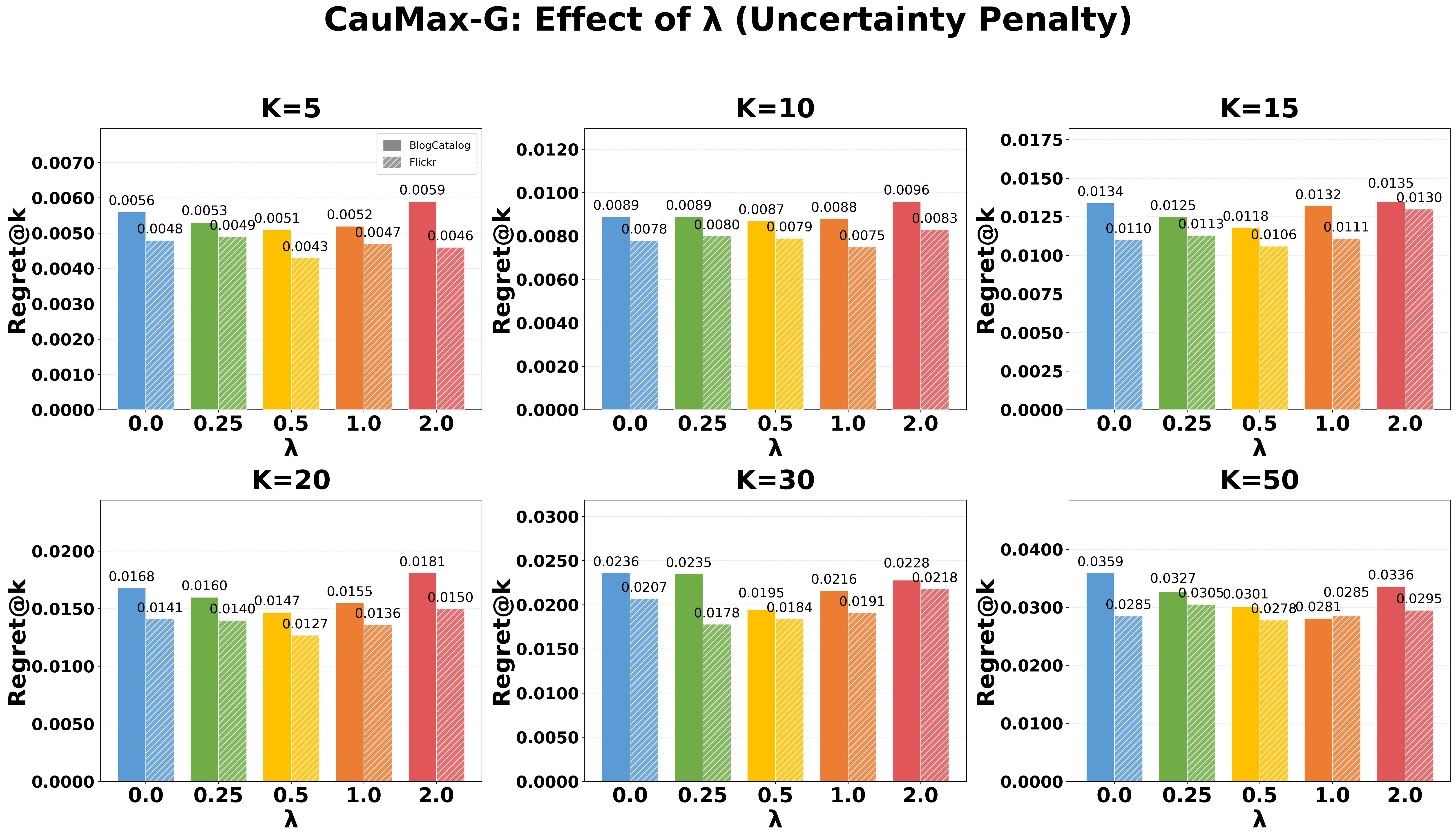
We vary $\lambda\in\{0,0.25,0.5,1.0,2.0\}$, where $\lambda=0$ reduces to the mean-only baseline, as shown in Figs. 3 and 4. Moderate penalization ($\lambda\in[0.25,0.5]$) consistently reduces regret across both datasets and search strategies; for CauMax-D, $\lambda=0.5$ reduces regret by up to 42% relative to $\lambda=0$. However, excessive penalization ($\lambda=2.0$) degrades performance by favoring low-variance subsets with smaller predicted effects. CauMax-D exhibits a stable U-shaped response with a clear optimum around $\lambda=0.5$, while CauMax-G shows a flatter profile, suggesting its iterative selection partially compensates for estimation noise even without explicit uncertainty penalization.

5.5. Computational Complexity

We analyze the time complexity of the proposed algorithms compared to the baselines, as summarized in Table 3. Let $|V_{A}|$ denote the number of source nodes, $|E|$ the number of edges, $K$ the budget, and $T_{\text{model}}$ the cost of a single forward pass through the estimator $f_{\theta}$. For the stochastic methods, $M$ represents the number of Monte Carlo dropout passes, and $R$ denotes the diffusion simulations in IM.

The CauMax-G (Algorithm 1) is computationally intensive; it requires $K$ iterations, where each iteration evaluates $|V_{A}|-|S|$ candidates via $M$ stochastic forward passes. This results in a complexity of $O(K\cdot|V_{A}|\cdot M\cdot T_{\text{model}})$. In contrast, the CauMax-D (Algorithm 2) runs for a fixed number of gradient steps $E_{\text{opt}}$, independent of the candidate set size during optimization, yielding $O(E_{\text{opt}}\cdot M\cdot T_{\text{model}})$. Since $E_{\text{opt}}\ll K\cdot|V_{A}|$ in practice, the differentiable method achieves a substantial speedup. Regarding baselines, Degree is highly efficient with $O(|V_{A}|\log|V_{A}|+|E|)$ due to sorting, while IM is expensive, scaling with the number of simulations $R$ and graph size.

Table 3. Comparison of time complexity for subset selection methods.

Method	Time Complexity
CauMax-G (Alg. 1)	$O(K\cdot|V_{A}|\cdot M\cdot T_{\mathrm{model}})$
CauMax-D (Alg. 2)	$O(E_{\mathrm{opt}}\cdot M\cdot T_{\mathrm{model}})$
Degree	$O(|V_{A}|\log|V_{A}|+|E|)$
IM	$O(K\cdot|V_{A}|\cdot R\cdot|E|)$
Random	$O(K)$

6. Conclusion

We introduced the problem of cross-group causal influence maximization, which seeks to identify the subset of source-group units whose intervention yields the greatest causal improvement in outcomes of a distinct target group connected through network interference pathways. We defined the core-to-group causal effect (Co2G) as a causal estimand grounded in the potential outcomes framework, and established its nonparametric identifiability from observational data via do-calculus. Building on this identification result, we proposed CauMax, a framework combining a graph neural network-based estimator that models within-group dependencies and cross-group spillover propagation with an uncertainty-aware optimization objective, instantiated through two scalable algorithms: CauMax-G (greedy search) and CauMax-D (differentiable optimization). Experiments on social network datasets confirmed that CauMax yields substantially lower regret than structural heuristics and diffusion-based baselines.

Limitations and Future Work

Our identification and estimation framework relies on the causal sufficiency assumption (Assumption 3.3), which requires that all common causes of source-group treatments and target-group outcomes are observed. In practice, unmeasured confounders such as latent homophily or unobserved socioeconomic factors may bias the estimated Co2G. Addressing hidden confounding is not the focus of this work, but it constitutes an important direction for future research. Potential approaches include incorporating proxy variables, instrumental variable methods, or sensitivity analysis to bound the impact of unobserved confounders on the estimated cross-group causal effects.