Neural Field Thermal Tomography: A Differentiable Physics Framework for Non-Destructive Evaluation

Abstract

We propose Neural Field Thermal Tomography (NeFTY), a differentiable physics framework for the quantitative 3D reconstruction of material properties from transient surface temperature measurements. While traditional thermography relies on pixel-wise 1D approximations that neglect lateral diffusion, and soft-constrained Physics-Informed Neural Networks (PINNs) often fail in transient diffusion scenarios due to gradient stiffness, NeFTY parameterizes the 3D diffusivity field as a continuous neural field optimized through a rigorous numerical solver. By leveraging a differentiable physics solver, our approach enforces thermodynamic laws as hard constraints while maintaining the memory efficiency required for high-resolution 3D tomography. Our discretize-then-optimize paradigm effectively mitigates the spectral bias and ill-posedness inherent in inverse heat conduction, enabling the recovery of subsurface defects at arbitrary scales. Experimental validation on synthetic data demonstrates that NeFTY significantly improves the accuracy of subsurface defect localization over baselines. Additional details at cab-lab-princeton.github.io/nefty.

1 Introduction

The quantitative characterization of subsurface material properties remains one of the most persistent challenges in the field of Non-Destructive Evaluation (NDE). As advanced manufacturing techniques, such as additive manufacturing and composite layups, produce increasingly complex geometries and material microstructures, the demand for high-resolution, volumetric inspection methods has intensified. Among the available modalities, active thermal inspection offers non-contact operation, scalability to large surfaces, and rapid data acquisition. As illustrated in Figure 1, by depositing a high-energy optical pulse onto a specimen’s surface and monitoring the subsequent temperature decay, one can theoretically infer the internal structure based on the transient thermal response. Discontinuities such as delaminations, voids, or inclusions disrupt the diffusive heat flux, manifesting as thermal contrast anomalies on the surface (Kovács et al., 2020; Rosa et al., 2025; Peng et al., 2025).

Figure 1: Overview of setup. A high-speed camera enables measurements of time-resolved transient surface temperature variations following localized heating with a pulsed laser. NeFTY uses these transient measurements to reconstruct the 3D subsurface diffusivity field and reveal hidden defects.

However, the transition from qualitative anomaly detection to quantitative Thermal Tomography, which is the reconstruction of 3D material property fields, specifically thermal diffusivity $\alpha(x,y,z)$, is hindered by the fundamental physics of heat transfer. Unlike wave propagation phenomena utilized in ultrasonics or radar (Burgholzer et al., 2018), which are governed by hyperbolic partial differential equations (PDEs) that preserve high-frequency information over distance, heat transfer is governed by a parabolic PDE (Vavilov et al., 1992). Diffusion is inherently a smoothing process. It acts as a stiff low-pass filter, causing high-frequency spatial details of internal features to decay exponentially with depth (Gahleitner et al., 2024). Consequently, the inverse heat conduction problem (IHCP) is severely ill-posed. Small perturbations in the measured surface temperature can correspond to arbitrarily large variations in the internal structure, particularly as depth increases (Qian et al., 2023; Leontiou et al., 2024).

Traditional approaches to this inverse problem have largely relied on signal processing heuristics or asymptotic approximations. Techniques such as Thermographic Signal Reconstruction (TSR) (Shepard et al., 2002) and Pulsed Phase Thermography (PPT) (Maldague et al., 2002) transform temporal data into domains (logarithmic derivatives or frequency phase) where defect contrast is enhanced. While effective for detecting the presence of defects, these methods typically employ 1D pixel-wise inversions that neglect lateral heat diffusion, leading to significant errors when estimating the size and depth of defects with low aspect ratios (Pérez et al., 2025). More advanced methods like the Virtual Wave Concept (VWC) (Burgholzer et al., 2017; Ali et al., 2025) attempt to mathematically transform the diffusive field into a pseudo-wave field to apply ultrasonic reconstruction algorithms.

In the parallel domain of computer vision and scientific machine learning, a paradigm shift has occurred with the introduction of Implicit Neural Representations (Sitzmann et al., 2020), or Neural Fields. The seminal work on Neural Radiance Fields (NeRF) (Mildenhall et al., 2021) demonstrated that complex 3D signals (density and color) could be parameterized not by a discrete voxel grid, but by a continuous coordinate-based neural network optimized via differentiable rendering. This analysis-by-synthesis approach solves the inverse problem by minimizing the discrepancy between observed images and those generated by the neural model. The success of NeRF has inspired a wave of applications in solving inverse problems in physics, from X-ray tomography (Xu et al., 2025; Zhou et al., 2025) to fluid dynamics (Kelly and Thurow, 2023).

To this end, we introduce Neural Field Thermal Tomography (NeFTY), a unified framework that translates the success of NeRF into the diffusive regime of thermal NDE. We formulate the reconstruction of the 3D thermal diffusivity field $\alpha(x,y,z)$ as a parameter estimation problem where the material property is represented by a neural network. Crucially, unlike black-box deep learning methods that attempt to learn a direct mapping from temperature to defects using massive training datasets (Kovács et al., 2020), NeFTY relies on Differentiable Physics. We integrate a differentiable numerical solver for the transient heat equation directly into the optimization loop. This allows the gradients of the reconstruction error with respect to the neural network weights to be computed exactly, enforcing the governing PDE as a hard constraint rather than a soft penalty.

Our contributions are summarized as follows:

• We propose NeFTY, a unified framework that couples implicit neural representations with differentiable physics, to solve the 3D inverse heat conduction problem, effectively capturing lateral diffusion effects neglected by traditional 1D heuristics.

• By employing a discretize-then-optimize approach with adjoint gradients, we strictly enforce thermodynamic laws as hard constraints to mitigate the optimization pathologies and spectral bias inherent in soft-constrained Physics-Informed Neural Networks (Raissi et al., 2019).

• We demonstrate that NeFTY achieves superior accuracy in recovering subsurface defect geometry through unsupervised test-time optimization, enabling generalization to novel geometries and materials without the need for labeled training data.

2 Related Work

Traditional Quantitative Thermography approaches have primarily relied on signal processing heuristics to enhance defect contrast, yet they often fundamentally neglect the three-dimensional nature of heat diffusion. Techniques such as TSR (Shepard et al., 2002; Shepard and Beemer, 2015) and PPT (Maldague et al., 2002; Chung et al., 2021) transform temporal decay data into logarithmic derivatives or frequency phase maps, effectively suppressing noise and mitigating emissivity variations. While these methods establish robust empirical relationships for depth estimation, such as the blind frequency approach (Ma et al., 2025), they typically treat each pixel as an isolated 1D thermal event, failing to account for the lateral heat diffusion that dominates around small or deep defects. Advanced mathematical transformations like VWC (Burgholzer et al., 2017; Schager et al., 2020; Ali et al., 2025) attempt to bridge this gap by remapping diffusion to pseudo-wave propagation for 3D reconstruction. However, this inverse mapping involves deconvolution operations that are severely ill-posed and amplify high-frequency measurement noise, often resulting in unstable reconstruction artifacts. In contrast, our approach embeds the full three-dimensional physics of heat diffusion directly into the inversion loop, naturally accounting for lateral flux without relying on asymptotic 1D approximations or heuristic transforms.

Deep Learning-based Frameworks have recently emerged as a candidate for solving inverse heat conduction problems (IHCP). Purely data-driven approaches using CNNs (Oliveira et al., 2021; Shi and Hsieh, 2021; Fang et al., 2023; Peng et al., 2025) have demonstrated success in defect detection, but their reliance on massive, labeled datasets renders them impractical for NDE, where obtaining ground truth requires expensive human supervision or destructive testing. Physics-Informed Neural Networks (PINNs) (Raissi et al., 2019; Cai et al., 2021; Leontiou et al., 2024) circumvent data scarcity by embedding the heat equation directly into the loss function. However, standard PINNs typically enforce physics as soft constraints via penalty terms (Leontiou et al., 2024), leading to significant optimization pathologies in transient diffusion problems. The inherent stiffness of the heat equation causes gradients to vanish for deep features, often resulting in spectral bias where networks fit surface boundary conditions while failing to resolve the high-frequency internal diffusivity structure (Wang et al., 2022; Hao et al., 2024). We address this by replacing the soft PDE constraint with a differentiable numerical solver, enforcing the physics as a hard constraint that guarantees thermodynamic consistency at every optimization step.

Neural Fields and Differentiable Physics, which combines the representational power of neural networks with the robustness of numerical solvers, has revolutionized parameter estimation in computer vision and is now permeating scientific computing. The seminal work on NeRF (Mildenhall et al., 2021) demonstrated that complex volumetric signals could be parameterized by continuous coordinate-based networks and optimized via differentiable ray-marching. This concept has been extended to scientific domains, such as X-ray tomography (Xu et al., 2025; Zhou et al., 2025) or fluid dynamics (Kelly and Thurow, 2023). Analogous to the differentiable rendering step in NeRF, differentiable physics approaches use exact discretized solvers to ensure that the physics is strictly satisfied at every optimization step. Consequently, these differentiable programming paradigms have found widespread adoption in scientific computing for solving PDEs (Holl et al., 2020; Holl and Thuerey, 2024; Bouziani et al., 2024), as well as in robotics and control systems (de Avila Belbute-Peres et al., 2018; Degrave et al., 2019; Turpin et al., 2023; Zhong and Allen-Blanchette, 2025). However, the application of these solver-in-the-loop methodologies to thermal non-destructive evaluation remains underexplored. NeFTY bridges this gap by unifying neural fields with a differentiable heat equation solver to efficiently compute gradients through the time-evolution of the physical system, thereby enabling high-fidelity, quantitative tomography from sparse surface measurements.

3 Preliminaries and Problem Statement

To ground the proposed framework, we first establish the mathematical formulation of the forward heat transfer process and rigorously define the inverse problem of thermal tomography.

3.1 The Forward Problem: Transient Heat Diffusion

We consider the thermal inspection of a solid object occupying a bounded spatial domain $\Omega\subset\mathbb{R}^{3}$, with boundary $\partial\Omega$. The physical process of interest is the transient diffusion of heat, which is governed by the conservation of energy and Fourier’s law of heat conduction. The evolution of the temperature field $T(\mathbf{x},t)$ for $\mathbf{x}=(x,y,z)\in\Omega$ and time $t\in[0,t_{\mathrm{end}}]$ is described by the parabolic PDE:

$$\frac{\partial T}{\partial t}=\nabla\cdot(\alpha(\mathbf{x})\nabla T)+S(\mathbf{x},t)\quad\text{in }\Omega\times(0,t_{\mathrm{end}}],$$ (1)

where $\alpha(\mathbf{x})$ is the thermal diffusivity ($\text{m}^{2}/\text{s}$), and $S(\mathbf{x},t)$ represents the normalized internal heat generation sources, which are typically zero in the passive cooling phase.

The system is closed by defining the initial state and boundary interactions. In a typical flash thermography setup, the object is initially at ambient temperature or in a steady state, followed by an instantaneous deposition of optical energy on its surface. We model this as an initial surface temperature distribution $T(\mathbf{x},0)=T_{0}(\mathbf{x})$ which decays over time. Following the flash pulse, we model the boundary conditions to approximate the inspection of a large, planar specimen. For the top and bottom surfaces ($\partial\Omega_{z}$), we assume adiabatic conditions to represent negligible convective losses during the short inspection window:

$$\mathbf{n}\cdot(\alpha\nabla T)=0\quad\text{on }\partial\Omega_{z},$$ (2)

where $\mathbf{n}$ denotes the outward unit normal vector to the boundary. For the lateral boundaries ($\partial\Omega_{xy}$), we employ Periodic Boundary Conditions. This effectively models a semi-infinite domain, mitigating numerical edge effects and reflections that would otherwise arise from the truncation of the simulation grid.

3.2 The Inverse Heat Conduction Problem (IHCP)

Figure 2: The Ill-Posedness of IHCP. Distinct internal structures (left), homogeneous vs. defective, produce nearly indistinguishable surface temperature profiles (right), illustrating the severe loss of high-frequency spatial information caused by diffusive smoothing.

Figure 3: Overview of NeFTY. Our method combines an implicit neural representation for the 3D diffusivity field with a differentiable physics solver. The network learns the internal structure by minimizing the error between simulated and measured surface temperatures, using the adjoint method for efficient gradient backpropagation through the transient thermal simulation.

The objective of Thermal Tomography is to recover the internal diffusivity field $\alpha(\mathbf{x})$ given measurements of the temperature evolution on a subset of the boundary. Let $\Gamma_{\mathrm{obs}}\subset\partial\Omega$ denote the observable surface (e.g., the front face accessible to the camera). The measurement data consists of a sequence of noisy temperature frames $\hat{T}(\mathbf{x}_{s},t_{i})$ acquired at discrete surface points $\mathbf{x}_{s}\in\Gamma_{\mathrm{obs}}$ and time steps $t_{i}\in\{t_{1},\dots,t_{M}\}$.

Formally, we seek the diffusivity field $\alpha^{*}$ that minimizes the discrepancy between the measured data and the solution of the forward model:

where $\mathcal{S}(\alpha)$ represents the forward operator (i.e., the solution $T(\mathbf{x},t)$ of the heat equation for a given field $\alpha$), $\mathcal{R}(\alpha)$ is a regularization functional necessary to constrain the solution space, $\lambda$ is a hyperparameter balancing data fidelity and regularity, and $\mathcal{A}$ is the bounded space of admissible diffusivity functions.

The Inverse Heat Conduction Problem is widely recognized as one of the most difficult inverse problems (Martinez Mundarain, 2024) in mathematical physics due to its severe ill-posedness, as characterized by Hadamard’s criteria (Hadamard, 1888). As illustrated in Figure 2, diffusion acts as a low-pass filter, causing distinct internal diffusivity configurations to yield nearly indistinguishable surface signatures. We discuss the mathematical challenges and Ill-Posedness of IHCP in Appendix A.

4 Method

We introduce NeFTY, a framework that synergizes the continuous parameterization of Neural Fields with the rigorous conservation laws of Differentiable Physics. As illustrated in Figure 3, the architecture consists of three tightly coupled components: (1) A Neural Field Representation that models the 3D diffusivity $\alpha(\mathbf{x})$; (2) A Differentiable Thermal Solver that simulates the transient heat diffusion; and (3) An Adjoint Optimization Loop that updates the neural representation by backpropagating surface errors through time.

4.1 Neural Parameterization of Diffusivity

Traditional thermal tomography relies on discrete voxel grids to store material properties. This discretization scales cubically with resolution ($\mathcal{O}(N^{3})$), creating a severe memory bottleneck that fundamentally limits the reconstruction of fine-scale defects. NeFTY overcomes this by replacing the discrete grid with a continuous function parameterized by a Multilayer Perceptron (MLP), $f_{\theta}:\mathbb{R}^{3}\to\mathbb{R}$.

Coordinate Mapping and Spectral Bias. Standard MLPs are known to suffer from spectral bias (Wang et al., 2022), effectively acting as low-pass filters that struggle to learn high-frequency functions such as the sharp boundaries of a subsurface void. To mitigate this, we lift the input coordinates $\mathbf{x}=(x,y,z)$ into a higher-dimensional feature space using a sinusoidal positional encoding $\gamma(\cdot)$. Following the standard NeRF formulation (Mildenhall et al., 2021), we employ log-linearly spaced frequencies:

where $L$ is a hyperparameter determining the bandwidth of the encoding. This mapping transforms the coordinate-based regression into a task suitable for the MLP, allowing the network to represent the sharp discontinuities characteristic of material defects (e.g., the interface between carbon fiber and an air void).

Network Architecture. The parameterized diffusivity field is modeled by a fully connected network. We employ ReLU activations (Nair and Hinton, 2010) for all hidden layers. To preserve gradient flow in deeper networks, we include skip connections that concatenate the input embedding $\gamma(\mathbf{x})$ to the features of selected intermediate layers.

Physical Constraints. To ensure the recovered parameters are physically admissible, we strictly constrain the output range. Thermal diffusivity must be positive to satisfy the Second Law of Thermodynamics, and effectively bounded for stable time-integration. We define the final diffusivity $\alpha_{\theta}(\mathbf{x})$ using a scaled Sigmoid activation:

$$\alpha_{\theta}(\mathbf{x})=\alpha_{\text{min}}+(\alpha_{\text{max}}-\alpha_{\text{min}})\cdot\sigma(f_{\theta}(\gamma(\mathbf{x}))),$$ (5)

where $\sigma(\cdot)$ is the logistic sigmoid function, and $[\alpha_{\text{min}},\alpha_{\text{max}}]$ defines the search window for admissible material properties. This hard-bracketing prevents the solver from encountering numerical instabilities caused by negative or exploding diffusivity values during the early phases of optimization.

4.2 Differentiable Forward Solver

The forward pass of NeFTY involves solving the transient heat equation using the diffusivity field predicted by the neural network. Unlike PINNs, which approximate the solution space directly with a network, we adopt a Discretize-then-Optimize paradigm (Onken and Ruthotto, 2020). We solve the PDE numerically using a differentiable discretization scheme, ensuring that physical conservation laws are strictly satisfied up to the precision of the grid.

Spatial Discretization. We leverage the Finite Difference Method and discretize the domain $\Omega$ into a uniform Cartesian grid. The continuous diffusivity field $\alpha_{\theta}(\mathbf{x})$ is sampled at the grid nodes. We approximate the spatial Laplacian $\nabla\cdot(\alpha\nabla T)$ using a standard second-order central difference stencil. For a node $(i,j,k)$, the diffusion term is approximated as:

where $\bar{\alpha}$ represents the effective diffusivity at the interface between nodes. A critical detail is the choice of interpolation for $\bar{\alpha}$. Standard arithmetic averaging ($\bar{\alpha}\approx(\alpha_{i}+\alpha_{i+1})/2$) is physically unsuitable for NDE as it smears out insulating boundaries (e.g., air voids) by allowing heat to leak through the interface. Instead, we employ the Harmonic Mean:

$$\bar{\alpha}_{i+1/2}=\frac{2\alpha_{i}\alpha_{i+1}}{\alpha_{i}+\alpha_{i+1}+\epsilon},$$ (7)

where $\epsilon$ is a small constant to prevent division by zero. The harmonic mean is dominated by the minimum value, correctly modeling the bottleneck effect of a resistive defect and preserving sharp thermal gradients at fracture boundaries.

Temporal Integration. Transient heat diffusion is a stiff PDE, particularly when diffusivity values vary by orders of magnitude (e.g., between air defects and bulk material). Explicit time-stepping schemes (e.g., Forward Euler) are bound by the Courant-Friedrichs-Lewy (CFL) condition (Courant et al., 1928), requiring prohibitively small time steps ($\Delta t<\Delta x^{2}/2\alpha_{max}$) to avoid divergence.

To decouple the simulation time step from the spatial resolution and material properties, NeFTY utilizes the Implicit Euler method. This method is unconditionally stable, allowing us to match the simulation step size $\Delta t$ to the experimental frame rate of the camera. The update from temperature state $\mathbf{T}^{n}$ to $\mathbf{T}^{n+1}$ is formulated as a linear system:

$$(\mathbf{I}-\Delta t\mathbf{L}(\alpha_{\theta}))\mathbf{T}^{n+1}=\mathbf{T}^{n},$$ (8)

where $\mathbf{I}$ is the identity matrix and $\mathbf{L}(\alpha_{\theta})$ is the discrete Laplacian operator constructed from the neural diffusivity field. We provide a rigorous mathematical derivation of the forward simulation scheme in Appendix B.

4.3 Optimization and Gradient Computation

The objective of NeFTY is to recover the unknown diffusivity parameters $\theta$ by minimizing the discrepancy between the simulated time-dependent surface temperature and the observed experimental data.

Loss Function. We define the loss $\mathcal{L}(\theta)$ as a combination of a data-fidelity term and a physics-inspired regularizer:

The data term $\mathcal{L}_{\text{data}}$ measures the Mean Squared Error (MSE) over $M$ time steps, where $\mathbf{M}$ is a binary mask isolating the valid sensor region and $\odot$ denotes element-wise multiplication. To mitigate the ill-posedness of the inverse problem, we apply Total Variation (TV) regularization (Rudin et al., 1992) on the predicted diffusivity field. This promotes piecewise-constant solutions, consistent with the physical expectation of distinct, homogeneous defects within a bulk material, and suppresses high-frequency noise artifacts.

Table 1: Quantitative comparison of 3D thermal diffusivity reconstruction. We evaluate reconstruction fidelity (MSE, PSNR, SSIM) and defect sizing accuracy (IoU) across both homogeneous and layered composite configurations. $\uparrow$ indicates higher is better; $\downarrow$ indicates lower is better. Best unsupervised results are highlighted in bold.

	Homogeneous				Layered Composite
Method	MSE ($10^{-4}$) $\downarrow$	PSNR $\uparrow$	SSIM $\uparrow$	IoU $\uparrow$	MSE ($10^{-4}$) $\downarrow$	PSNR $\uparrow$	SSIM $\uparrow$	IoU $\uparrow$
Supervised
U-Net (Full)	0.96$\pm$0.11	24.20$\pm$0.45	0.94$\pm$0.01	0.70$\pm$0.02	3.36$\pm$0.71	20.03$\pm$0.80	0.90$\pm$0.01	0.68$\pm$0.03
U-Net (Sound-Only)	14.73$\pm$3.83	14.83$\pm$0.71	0.83$\pm$0.02	0.00$\pm$0.00	10.17$\pm$2.21	15.42$\pm$0.98	0.88$\pm$0.02	0.00$\pm$0.00
Unsupervised
Grid Opt.	12.61$\pm$4.20	13.99$\pm$1.18	0.56$\pm$0.04	0.04$\pm$0.02	15.01$\pm$2.97	13.27$\pm$0.88	0.57$\pm$0.04	0.03$\pm$0.01
PINN	208.3$\pm$26.2	-0.24$\pm$0.06	0.04$\pm$0.01	0.01$\pm$0.00	200.3$\pm$17.8	1.42$\pm$0.27	0.04$\pm$0.01	0.02$\pm$0.00
NeFTY Ablations
Base	127.4$\pm$92.2	0.47$\pm$3.17	0.28$\pm$0.05	0.03$\pm$0.02	221.6$\pm$130.5	2.89$\pm$1.88	0.24$\pm$0.05	0.02$\pm$0.02
+ PE	126.1$\pm$59.4	4.17$\pm$1.36	0.12$\pm$0.02	0.09$\pm$0.03	87.16$\pm$29.71	6.15$\pm$1.11	0.13$\pm$0.02	0.09$\pm$0.03
+ PE, FA	29.80$\pm$4.78	8.33$\pm$0.59	0.16$\pm$0.02	0.14$\pm$0.03	44.33$\pm$15.94	8.81$\pm$0.87	0.18$\pm$0.03	0.14$\pm$0.03
+ PE, FA, $\sigma$	31.43$\pm$8.58	9.19$\pm$0.94	0.26$\pm$0.03	0.18$\pm$0.04	35.60$\pm$6.07	9.27$\pm$0.82	0.24$\pm$0.04	0.14$\pm$0.04
+ PE, FA, $\sigma$, HM	21.01$\pm$5.67	10.95$\pm$0.94	0.36$\pm$0.03	0.24$\pm$0.05	23.09$\pm$4.77	11.26$\pm$0.84	0.33$\pm$0.05	0.22$\pm$0.06
NeFTY (Ours)	3.66$\pm$1.31	18.48$\pm$0.53	0.77$\pm$0.02	0.45$\pm$0.04	9.26$\pm$2.81	15.88$\pm$0.79	0.74$\pm$0.03	0.37$\pm$0.06

Differentiable Physics. Optimizing $\theta$ requires computing the gradient $\nabla_{\theta}\mathcal{L}$. Applying the chain rule reveals the computational bottleneck:

$$\frac{d\mathcal{L}}{d\theta}=\sum_{t=1}^{M}\frac{\partial\mathcal{L}}{\partial\mathbf{T}^{t}}\frac{\partial\mathbf{T}^{t}}{\partial\alpha}\frac{\partial\alpha}{\partial\theta}.$$ (10)

The term $\frac{\partial\mathbf{T}^{t}}{\partial\alpha}$ represents the sensitivity of the temperature history to the diffusivity field. Computing this via standard Backpropagation Through Time (BPTT) requires differentiating through the PDE solver at every time step. This necessitates storing the intermediate temperature states $\mathbf{T}^{t}$ for all $t=1\dots M$ to compute the backward pass. For high-resolution 3D tomography, this memory cost is prohibitive. For example, a standard grid of $128^{3}$ voxels simulated over $1000$ time steps would require terabytes of GPU memory to store the computational graph, rendering BPTT infeasible.

To overcome this memory bottleneck, we leverage the implicit function theorem (adjoint method) (Céa, 1986). Modern automatic differentiation frameworks (Bradbury et al., 2018; Paszke et al., 2019; Schoenholz and Cubuk, 2020) efficiently handle this by solving an auxiliary linear system during the backward pass. For a linear system $\mathbf{A}\mathbf{x}=\mathbf{b}$, the gradient of the solution $\mathbf{x}$ with respect to the system matrix $\mathbf{A}$ (which depends on $\theta$) is computed by solving:

$$\mathbf{A}^{T}\boldsymbol{\lambda}=\frac{\partial\mathcal{L}}{\partial\mathbf{x}},$$ (11)

where $\boldsymbol{\lambda}$ is the adjoint variable. This allows NeFTY to compute exact gradients for the diffusivity field without storing the intermediate states of the forward solver, enabling high-resolution 3D reconstruction on standard GPU hardware. We provide the full derivation of the adjoint formulation in Appendix C.

Frequency Annealing. The inverse heat conduction problem is non-convex. To avoid local minima, we implement a coarse-to-fine Frequency Annealing strategy during training (Park et al., 2021). We begin optimization with a low-bandwidth Fourier mapping, forcing the network to prioritize global, low-frequency thermal properties (bulk conductivity). As training progresses, we gradually unlock higher frequency bands in the encoding $\gamma(\mathbf{x})$. We modulate the $k$-th frequency band with a weight $w_{k}(\beta)$:

$$w_{k}(\beta)=\frac{1-\cos(\pi\cdot\text{clamp}(\beta-k,0,1))}{2},$$ (12)

where $\beta(t)$ is a parameter that increases linearly from $0$ to the maximum frequency $L$ over the initial phase of training. This soft-masking approach prevents abrupt gradients associated with binary masking, allowing the network to stably grow high-frequency details and sharpen defect boundaries.

5 Experiments

Figure 4: Depth-wise slices of the recovered diffusivity field (Homogeneous Setting). NeFTY (Ours) successfully localizes and sizes the subsurface defects (red/blue shapes) with sharp boundaries. The PINN baseline saturates to a trivial solution due to gradient pathology. The Grid Opt. baseline is physically consistent but noisy. The Sound-Only U-Net fails to detect the OOD defects.

5.1 Experimental Settings

To rigorously evaluate the reconstruction fidelity of NeFTY and ensure a fair comparison, we strictly avoid the inverse crime of generating data with the same numerical scheme used for inversion. Instead, we generate a large-scale synthetic dataset using PhiFlow (Holl and Thuerey, 2024), a distinct Finite Volume Method (FVM) physics engine. While our reconstruction framework uses an implicit solver for gradient stability, the ground-truth data are generated using a high-fidelity explicit diffusion scheme with adaptive substepping to ensure physical accuracy.

We simulate a quasi-2D specimen with unitless dimensions of $10\times 10\times 1$, discretized into a $64\times 64\times 16$ grid. The dataset comprises 1,000 samples split into two configurations: a Homogeneous setting, where the bulk material has uniform diffusivity $\alpha_{\mathrm{base}}$, and a Layered setting, simulating a composite with varying $\alpha_{\mathrm{base}}$ across 3 to 4 layers along the z-axis. Each sample contains 1 to 4 subsurface defects (ellipsoid, cylinder, or box) buried at varying depths. We record the thermal response over 100 time steps ($\Delta t=0.05$). To ensure stability and precision in the ground truth generation, we dynamically calculate the Courant-Friedrichs-Lewy (CFL) (Courant et al., 1928) limit and apply a variable number of explicit substeps (typically $>10$) per recorded frame. Material properties are sampled from Uniform distributions, with $\alpha_{\mathrm{base}}\sim\mathcal{U}(0.1,0.2)$ and $\alpha_{\mathrm{defect}}\sim\mathcal{U}(0.005,0.015)$. A detailed dimensional analysis connecting these unitless parameters to physical scales is provided in Appendix D.1.

We benchmark NeFTY against four baselines: (1) Voxel-Grid Optimization (direct $\alpha$ tensor optimization without neural priors); (2) Physics-Informed Neural Networks (PINNs) (soft-penalty formulation); (3) End-to-End Thermal U-Net (supervised 3D CNN) (Ronneberger et al., 2015); and (4) U-Net (Sound-Only), trained exclusively on defect-free samples. We emphasize that the U-Net serves as a soft theoretical upper bound on performance, as it is trained under full supervision on the ground-truth $\alpha$ fields, which is typicallly unavailable in real-world NDE scenarios. The Sound-Only baseline evaluates the generalization capability of data-driven methods when defects represent out-of-distribution anomalies. To isolate the efficacy of our proposed mechanisms, we evaluate a series of cumulative ablations starting from a naively implemented neural field. This begins with a Base model (raw coordinates, arithmetic mean, softplus activation, no regularization) and incrementally incorporates Positional Encoding (+PE), Frequency Annealing (+FA), Sigmoid constraints (+$\sigma$), and Harmonic Mean discretization (+HM), culminating in the full NeFTY framework. We evaluate performance using Mean Squared Error (MSE) for surface data fidelity, Peak Signal-to-Noise Ratio (PSNR) and Structural Similarity Index (SSIM) (Wang et al., 2004) for $\alpha$ reconstruction quality, and volumetric Intersection over Union (IoU) for defect sizing (threshold $\alpha<0.03$). Implementation details for all baselines are in Appendix D.2.

5.2 Comparative Reconstruction Results

Figure 5: Qualitative Results (Layered Composite Setting). Comparison of reconstruction quality in a multi-layered material. NeFTY correctly resolves both the layer transitions and the embedded defects. The baselines struggle with the complex heterogeneity. Grid Opt. introduces significant artifacts at layer interfaces, while the PINN again fails to converge to a meaningful structure.

Quantitative Performance. As detailed in Table 1, NeFTY outperforms all unsupervised baselines, achieving an order-of-magnitude reduction in MSE and superior defect sizing accuracy (IoU). The Standard PINN fails to converge to meaningful solutions (IoU $\approx 0.01$) due to the gradient stiffness inherent in the soft PDE constraint, validating our theoretical analysis in Appendix A. While the Full U-Net provides a strong upper bound (IoU 0.70) under full supervision, its performance collapses (IoU 0.00) in the Sound-Only setting when facing out-of-distribution defects. NeFTY bridges this gap, achieving robust localization (IoU 0.45) comparable to supervised methods without requiring defect labels. We provide extended quantitative analysis, including depth-wise error metrics and additional qualitative examples, in Appendix E.

Qualitative Analysis. Figures 4 and 5 present 3D reconstruction and depth-wise cross-sections of the reconstructed diffusivity fields. NeFTY recovers the sharp boundaries of subsurface defects with high contrast, closely matching the Ground Truth geometry. The Grid Optimization baseline exhibits characteristic ringing artifacts and noise, obscuring the defect shapes. The PINN output is featureless, reflecting its convergence to a trivial local minimum. The Sound-Only U-Net reconstructs the bulk material but ghosts the defects entirely, treating them as noise.

Ablation Study. The cumulative improvements shown in Table 1 validate our architectural choices. The Base neural field fails to resolve high-frequency defects. Adding PE and FA stabilizes the learning of sharp features, while the HM and Sigmoid (+$\sigma$) constraints are critical for physical plausibility. The final addition of TV regularization in the full NeFTY model yields the definitive leap in IoU, suppressing noise while preserving sharp defect interfaces.

5.3 Computational Efficiency

Table 2: Computational efficiency benchmark on a single sample. We compare our differentiable solver (implemented via Adjoint method (AM) vs. standard Autograd (AD)) against the PhiFlow physics engine. Ours (Adjoint) achieves orders-of-magnitude lower memory consumption compared to Autograd.

Method	Fwd Time (s) $\downarrow$	Bwd Time (s) $\downarrow$	Peak Mem $\downarrow$	Sim. Error $\downarrow$
PhiFlow (Ex)	$26.36\pm 0.10$	$0.87\pm 0.01$	3.26 GB	$7.91\times 10^{-4}$
PhiFlow (Im)	$3.26\pm 0.40$	$0.76\pm 0.01$	275.5 MB	$8.47\times 10^{-4}$
Ours (AD)	$1.43\pm 0.04$	$1.30\pm 0.02$	18.63 GB	3.73 $\mathbf{\times 10^{-8}}$
Ours (AM)	0.46 $\pm$ 0.00	0.50 $\pm$ 0.00	21.9 MB	3.73 $\mathbf{\times 10^{-8}}$

To validate the scalability of our approach, we benchmark the computational performance of our differentiable solver against the PhiFlow (Holl and Thuerey, 2024) physics engine on a single $64\times 64\times 16$ simulation sample over 50 time steps. As shown in Table 2, our implementation utilizing the Adjoint Method (AM) significantly outperforms standard Autograd (AD) and baseline solvers. By avoiding the storage of intermediate states required by Backpropagation Through Time, Ours (AM) reduces peak memory consumption from 18.63 GB (AD) to just 21.9 MB, enabling high-resolution 3D inversion on standard hardware. Furthermore, our solver achieves a forward pass time of 0.46s, an $\sim$7$\times$ speedup over PhiFlow’s implicit solver, while maintaining high numerical precision (Sim. Error $\approx 10^{-8}$) relative to an exact Scipy CPU reference. This efficiency is critical for the iterative optimization loop required by NeFTY.

6 Conclusion

We present Neural Field Thermal Tomography (NeFTY), a unified framework that resolves the ill-posed inverse heat conduction problem by bridging implicit neural representations with differentiable physics. By enforcing the governing PDE as a hard constraint via a rigorous numerical solver, NeFTY overcomes the optimization pathologies and spectral bias that plague soft-constrained PINNs in stiff diffusive regimes. Our results demonstrate that this discretize-then-optimize paradigm, enabled by memory-efficient adjoint gradients and frequency annealing, achieves superior 3D reconstruction fidelity compared to both classical heuristics and data-driven baselines without requiring labeled supervision.

Impact Statement

This paper presents work whose goal is to advance the field of Machine Learning. There are many potential societal consequences of our work, none which we feel must be specifically highlighted here.

Appendix A Mathematical Challenges and Ill-Posedness of IHCP

We provide a formal analysis of the Inverse Heat Conduction Problem (IHCP) to elucidate the necessity of the hard-constraint differentiable physics approach employed in NeFTY.

A.1 Hadamard’s Ill-Posedness and Compact Operators

The forward problem of transient heat conduction can be abstractly defined as an operator equation. Let $X=L^{2}(\Omega)$ represent the space of initial conditions or internal diffusivity distributions, and $Y=L^{2}(\partial\Omega\times)$ represent the space of surface temperature measurements. The forward operator $\mathcal{K}:X\to Y$ maps the internal parameters to the boundary trace solution of the parabolic PDE:

$$\mathcal{K}(\alpha)=T|_{\partial\Omega}.$$ (13)

The inverse problem seeks to recover $\alpha$ given noisy measurements $y^{\delta}$ such that $\|y^{\delta}-y_{true}\|\leq\delta$. According to Hadamard (1888), a problem is well-posed if a solution exists, is unique, and depends continuously on the data. The IHCP fails the stability condition (continuous dependence) due to the properties of $\mathcal{K}$.

For diffusion processes, $\mathcal{K}$ is a compact operator. The singular value decomposition (SVD) of a compact operator yields a sequence of singular values $\{\sigma_{n}\}$ that decay to zero. For the heat equation, this decay is exponential with respect to the frequency of the spatial modes. Consider a perturbation in the internal parameter $\delta\alpha_{n}$ corresponding to a spatial frequency $n$. The resulting perturbation in the surface temperature is damped by a factor proportional to:

$$\sigma_{n}\sim e^{-n^{2}\pi^{2}t}.$$ (14)

Recovering $\alpha$ requires inverting this operator. The inverse operator $\mathcal{K}^{-1}$ is unbounded because the singular values of the inverse are $\sigma_{n}^{-1}\sim e^{n^{2}\pi^{2}t}$. Consequently, high-frequency noise components in the measurement $y^{\delta}$ are amplified exponentially, rendering the naive inversion unstable. This necessitates regularization, which NeFTY imposes via the implicit neural representation (acting as a deep prior) and the total variation penalty.

A.2 Optimization Pathology in Soft-Constrained PINNs

A standard Physics-Informed Neural Network (PINN) approximates the solution $T_{\theta}(\mathbf{x},t)$ and diffusivity $\alpha_{\phi}(\mathbf{x})$ by minimizing a composite loss functional $\mathcal{L}_{\mathrm{PINN}}$:

$$\mathcal{L}_{\mathrm{PINN}}(\theta,\phi)=\underbrace{\|T_{\theta}-\hat{T}\|_{\Gamma_{\mathrm{obs}}}^{2}}_{\mathcal{L}_{\mathrm{data}}}+\lambda\underbrace{\|\partial_{t}T_{\theta}-\nabla\cdot(\alpha_{\phi}\nabla T_{\theta})\|_{\Omega}^{2}}_{\mathcal{L}_{\mathrm{PDE}}}.$$ (15)

This soft constraint formulation suffers from severe gradient pathology in transient diffusion regimes. Let $g_{\mathrm{data}}=\nabla_{\phi}\mathcal{L}_{\mathrm{data}}$ and $g_{\mathrm{PDE}}=\nabla_{\phi}\mathcal{L}_{\mathrm{PDE}}$. The sensitivity of the boundary data to deep internal parameters is exponentially small (as shown in A.1). Thus, $\|g_{\mathrm{data}}\|\ll\|g_{\mathrm{PDE}}\|$ for parameters far from the boundary. During gradient descent, the optimization is dominated by the PDE residual term (ensuring the equation holds locally) rather than the data term (ensuring the parameters match reality). This often leads to trivial solutions where $\mathcal{L}_{\mathrm{PDE}}\approx 0$ but data fit is poor, or requires manual, delicate tuning of the penalty weight $\lambda$.

Further, neural networks exhibit a spectral bias, converging to low-frequency components of the target function first. In the context of the heat equation, the PDE residual loss $\mathcal{L}_{\mathrm{PDE}}$ involves second-order spatial derivatives $\Delta T$, which amplify high-frequency errors in the network approximation. The network struggles to eliminate these high-frequency residual errors, leading to ghosting artifacts and an inability to resolve sharp defect boundaries.

A.3 Regularization via Hard Constraints

NeFTY reformulates the problem as a PDE-constrained optimization problem where the physics is satisfied exactly (up to discretization error) at every optimization step $k$. We treat the temperature $\mathbf{T}$ not as a free parameter of a network, but as an implicit function of the diffusivity $\alpha_{\theta}$, defined by the solution of the discretized state equation $F(T,\alpha_{\theta})=0$. The optimization problem becomes:

$$\min_{\theta}\mathcal{L}(\mathbf{T}(\alpha_{\theta}))\quad\text{subject to}\quad F(\mathbf{T},\alpha_{\theta})=0.$$ (16)

The gradient with respect to network weights $\theta$ is computed via the Adjoint State Method. Let $\mathcal{L}$ be the objective function. By the Chain Rule and the Implicit Function Theorem:

$$\frac{d\mathcal{L}}{d\theta}=\frac{\partial\mathcal{L}}{\partial\mathbf{T}}\frac{d\mathbf{T}}{d\alpha}\frac{\partial\alpha}{\partial\theta}=\lambda^{T}\frac{\partial F}{\partial\alpha}\frac{\partial\alpha}{\partial\theta},$$ (17)

where the adjoint variable $\lambda$ is the solution to the linear system:

$$\left(\frac{\partial F}{\partial\mathbf{T}}\right)^{T}\lambda=-\left(\frac{\partial\mathcal{L}}{\partial\mathbf{T}}\right)^{T}.$$ (18)

Crucially, $\frac{\partial F}{\partial\mathbf{T}}$ is the Jacobian of the discretized heat operator (typically a discrete Laplacian matrix). Inverting this matrix (or solving the linear system) mathematically corresponds to back-propagating information from the sensor boundary into the domain, explicitly reversing the diffusion process in a physically consistent manner. This ensures that gradients $\frac{d\mathcal{L}}{d\theta}$ correctly reflect the causal relationship between internal defects and surface observations, avoiding the vanishing gradient issues inherent to the soft-penalty formulation.

Appendix B Discrete Forward Simulation

In this section, we provide the detailed derivation of the numerical scheme used in NeFTY to solve the transient heat conduction equation. We employ a Finite Difference Method (FDM) for spatial discretization and the Implicit Euler method for temporal integration. This combination ensures unconditional stability regardless of the time step size or diffusivity contrast. Verification of our simulator is shown in Appendix F.

B.1 Governing Equations and Normalization

The governing partial differential equation (PDE) for heat transfer in an isotropic medium is:

$$\rho C_{p}\frac{\partial T}{\partial t}=\nabla\cdot(k(\mathbf{x})\nabla T)+Q(\mathbf{x},t),$$ (19)

where $\rho$ is density, $C_{p}$ is specific heat capacity, and $k(\mathbf{x})$ is thermal conductivity. Dividing by the volumetric heat capacity $\rho C_{p}$, we obtain the normalized form parameterized by thermal diffusivity $\alpha(\mathbf{x})=\frac{k(\mathbf{x})}{\rho C_{p}}$:

$$\frac{\partial T}{\partial t}=\nabla\cdot(\alpha(\mathbf{x})\nabla T)+S(\mathbf{x},t),$$ (20)

where $S(\mathbf{x},t)$ is the normalized source term.

B.2 Temporal Discretization (Implicit Euler)

We discretize the time domain into $N_{t}$ steps of size $\Delta t$. Let $\mathbf{T}^{n}$ denote the discretized temperature field at time $t=n\Delta t$. Using the Backward Differentiation Formula (Implicit Euler), the time derivative is approximated as:

$$\frac{\mathbf{T}^{n+1}-\mathbf{T}^{n}}{\Delta t}=\mathcal{D}(\alpha)\mathbf{T}^{n+1}+\mathbf{S}^{n+1},$$ (21)

where $\mathcal{D}(\alpha)$ is the spatial differential operator. Rearranging terms separates the known state $\mathbf{T}^{n}$ from the unknown future state $\mathbf{T}^{n+1}$:

$$(\mathbf{I}-\Delta t\mathcal{D}(\alpha))\mathbf{T}^{n+1}=\mathbf{T}^{n}+\Delta t\mathbf{S}^{n+1}.$$ (22)

This requires solving a linear system at every time step. While computationally more expensive than explicit stepping, it bypasses the strict CFL condition ($\Delta t<\frac{\Delta x^{2}}{2\alpha}$) (Courant et al., 1928), allowing for larger steps consistent with experimental frame rates.

B.3 Spatial Discretization (FDM)

We discretize the domain $\Omega$ into a uniform Cartesian grid with spacing $\Delta x,\Delta y,\Delta z$. The continuous operator $\nabla\cdot(\alpha\nabla T)$ is approximated using a second-order central difference stencil.

To maintain conservation of heat flux across material interfaces, particularly those with high contrast (e.g., polymer-air boundaries), we define the effective diffusivity at cell faces using the Harmonic Mean. For a node $(i,j,k)$, the effective diffusivity $\bar{\alpha}_{i+1/2}$ at the interface with $(i+1,j,k)$ is:

$$\bar{\alpha}_{i+1/2}=\frac{2\alpha_{i,j,k}\alpha_{i+1,j,k}}{\alpha_{i,j,k}+\alpha_{i+1,j,k}}.$$ (23)

Unlike the arithmetic mean, the harmonic mean is dominated by the lower diffusivity value, allowing the solver to correctly model the ”throttling” of heat flux caused by insulating defects. The full discrete Laplacian operator $\mathbf{L}(\alpha)\mathbf{T}$ is given by:

$$\begin{split}\mathbf{L}(\alpha)\mathbf{T}]_{i,j,k}\approx&\frac{1}{\Delta x^{2}}\left[\bar{\alpha}_{i+1/2}(T_{i+1,j,k}-T_{i,j,k})-\bar{\alpha}_{i-1/2}(T_{i,j,k}-T_{i-1,j,k})\right]\\ +&\frac{1}{\Delta y^{2}}\left[\bar{\alpha}_{j+1/2}(T_{i,j+1,k}-T_{i,j,k})-\bar{\alpha}_{j-1/2}(T_{i,j,k}-T_{i,j-1,k})\right]\\ +&\frac{1}{\Delta z^{2}}\left[\bar{\alpha}_{k+1/2}(T_{i,j,k+1}-T_{i,j,k})-\bar{\alpha}_{k-1/2}(T_{i,j,k}-T_{i,j,k-1})\right].\end{split}$$ (24)

For the lateral dimensions ($x,y$), we handle boundary connectivity via periodic wrapping (circular padding), while for the depth dimension ($z$), we employ replicate padding to enforce the Neumann zero-flux constraint.

B.4 The Linear System

Combining B.2 and B.3, the update rule becomes a sparse linear system of the form $\mathbf{A}\mathbf{x}=\mathbf{b}$:

$$\underbrace{(\mathbf{I}-\Delta t\mathbf{L}(\alpha))}_{\mathbf{A}(\alpha)}\mathbf{T}^{n+1}=\underbrace{\mathbf{T}^{n}+\Delta t\mathbf{S}^{n+1}}_{\mathbf{b}}.$$ (25)

The system matrix $\mathbf{A}(\alpha)$ is sparse, symmetric (assuming adiabatic or constant-temperature boundaries), and positive-definite, allowing for efficient solution via Preconditioned Conjugate Gradient (Hestenes et al., 1952) or iterative methods. To maintain a fully differentiable computational graph on the GPU without relying on complex sparse matrix decompositions, we solve this system using the Jacobi Iteration method.

We decompose $\mathbf{A}$ into its diagonal component $\mathbf{D}$ and off-diagonal remainder $\mathbf{R}$ such that $\mathbf{A}=\mathbf{D}+\mathbf{R}$. The solution $\mathbf{T}^{n+1}$ is approximated by unrolling a fixed number of iterations $K$ (e.g., $K=50$ in our experiments). The update rule for the $k$-th iteration is:

$$\mathbf{T}^{(k+1)}=\mathbf{D}^{-1}\left(\mathbf{b}-\mathbf{R}\mathbf{T}^{(k)}\right).$$ (26)

This formulation allows the solver to be implemented entirely via efficient tensor operations (convolutions or stencils), facilitating seamless integration with automatic differentiation frameworks.

Appendix C Gradient Derivation via Adjoint State Method

Optimizing the neural field parameters $\theta$ requires computing the gradient of the loss function $\mathcal{L}$ with respect to $\theta$. Because the forward pass involves solving a linear system at each time step, standard backpropagation (BPTT) would require storing the entire computational graph (all intermediate $\mathbf{T}^{n}$ and solver steps), leading to prohibitive memory usage. We instead utilize the Adjoint State Method to compute gradients with constant memory cost with respect to time steps.

C.1 The Constrained Optimization Problem

We aim to minimize the cumulative loss $\mathcal{L}=\sum_{n=1}^{N_{t}}\ell(\mathbf{T}^{n})$, subject to the physics constraints. We define the residual function $\mathbf{F}^{n}$ for the $n$-th time step as:

$$\mathbf{F}^{n}(\mathbf{T}^{n},\mathbf{T}^{n-1},\alpha)=\mathbf{A}(\alpha)\mathbf{T}^{n}-\mathbf{T}^{n-1}-\Delta t\mathbf{S}^{n}=\mathbf{0},$$ (27)

where $\mathbf{A}(\alpha)=\mathbf{I}-\Delta t\mathbf{L}(\alpha)$.

C.2 Adjoint Recurrence Relation

We introduce a sequence of Lagrange multipliers (adjoint variables) $\boldsymbol{\lambda}^{n}$ for each time step. The augmented Lagrangian is:

$$\mathcal{J}=\sum_{n=1}^{N_{t}}\ell(\mathbf{T}^{n})-\sum_{n=1}^{N_{t}}(\boldsymbol{\lambda}^{n})^{\top}\mathbf{F}^{n}(\mathbf{T}^{n},\mathbf{T}^{n-1},\alpha).$$ (28)

Setting the total derivative of $\mathcal{J}$ with respect to the state variable $\mathbf{T}^{n}$ to zero yields the Adjoint Equation (backward-in-time recurrence):

$$\frac{\partial\mathcal{J}}{\partial\mathbf{T}^{n}}=\frac{\partial\ell}{\partial\mathbf{T}^{n}}-(\boldsymbol{\lambda}^{n})^{\top}\frac{\partial\mathbf{F}^{n}}{\partial\mathbf{T}^{n}}-(\boldsymbol{\lambda}^{n+1})^{\top}\frac{\partial\mathbf{F}^{n+1}}{\partial\mathbf{T}^{n}}=0.$$ (29)

Substituting the partial derivatives of the residual $\mathbf{F}$:

$$\begin{split}\frac{\partial\mathbf{F}^{n}}{\partial\mathbf{T}^{n}}&=\mathbf{A}(\alpha)\\ \frac{\partial\mathbf{F}^{n+1}}{\partial\mathbf{T}^{n}}&=-\mathbf{I}.\end{split}$$ (30)

We obtain the linear system for the adjoint variable $\boldsymbol{\lambda}^{n}$:

$$\mathbf{A}(\alpha)^{\top}\boldsymbol{\lambda}^{n}=\left(\frac{\partial\ell}{\partial\mathbf{T}^{n}}\right)^{\top}+\boldsymbol{\lambda}^{n+1},$$ (31)

with the terminal condition $\boldsymbol{\lambda}^{N_{t}+1}=\mathbf{0}$. Crucially, solving this system involves the transpose of the same sparse matrix $\mathbf{A}$ used in the forward pass. This means the adjoint states $\boldsymbol{\lambda}^{n}$ can be computed iteratively backwards from $n=N_{t}$ to $1$.

C.3 Gradient with Respect to Parameters

Once the adjoint variables $\boldsymbol{\lambda}^{n}$ are computed, the gradient of the loss with respect to the diffusivity field $\alpha$ is given by the sum of contributions from all time steps:

$$\frac{d\mathcal{L}}{d\alpha}=-\sum_{n=1}^{N_{t}}(\boldsymbol{\lambda}^{n})^{\top}\frac{\partial\mathbf{F}^{n}}{\partial\alpha}.$$ (32)

Recall that $\mathbf{F}^{n}=(\mathbf{I}-\Delta t\mathbf{L}(\alpha))\mathbf{T}^{n}-\mathbf{T}^{n-1}$. The derivative with respect to $\alpha$ acts only on the Laplacian matrix $\mathbf{L}(\alpha)$:

$$\frac{\partial\mathbf{F}^{n}}{\partial\alpha}=-\Delta t\frac{\partial(\mathbf{L}(\alpha)\mathbf{T}^{n})}{\partial\alpha}.$$ (33)

Thus, the final gradient is:

$$\frac{d\mathcal{L}}{d\alpha}=\Delta t\sum_{n=1}^{N_{t}}(\boldsymbol{\lambda}^{n})^{\top}\frac{\partial(\mathbf{L}(\alpha)\mathbf{T}^{n})}{\partial\alpha}.$$ (34)

Finally, the gradient with respect to the neural network weights $\theta$ is computed via the chain rule:

$$\frac{d\mathcal{L}}{d\theta}=\left(\frac{d\mathcal{L}}{d\alpha}\right)^{\top}\frac{\partial\alpha_{\theta}}{\partial\theta}.$$ (35)

This formulation allows us to compute exact gradients by running one forward simulation (to get $\mathbf{T}^{n}$) and one backward adjoint simulation (to get $\boldsymbol{\lambda}^{n}$), requiring memory only for the current state, regardless of the number of time steps.

C.4 Sensitivity to Initial Conditions

In scenarios where the initial temperature $\mathbf{T}^{0}$ is also a learnable parameter or uncertain, we can compute the sensitivity using the adjoint state at the first time step. Following the recurrence relation to $n=1$, the gradient w.r.t. $\mathbf{T}^{0}$ is:

$$\frac{d\mathcal{L}}{d\mathbf{T}^{0}}=(\boldsymbol{\lambda}^{1})^{\top}\frac{\partial\mathbf{F}^{1}}{\partial\mathbf{T}^{0}}=(\boldsymbol{\lambda}^{1})^{\top}(-\mathbf{I})=-\boldsymbol{\lambda}^{1}.$$ (36)

This result provides a direct mechanism to optimize initial conditions simultaneously with material properties.

Appendix D Experimental Details

D.1 Ground Truth Generation and Physical Scaling

Ground Truth Generation Strategy. To maintain rigorous methodological independence and avoid the inverse crime of generating data with the same numerical model used for reconstruction, we utilize PhiFlow (Holl and Thuerey, 2024), a distinct Finite Volume Method (FVM) physics engine, for all ground truth data generation. While the NeFTY reconstruction framework employs an implicit solver to enable large time steps and gradient stability during optimization, the ground truth data is generated using a high-fidelity explicit diffusion scheme. To overcome the stability constraints inherent to explicit integration on fine grids, we implement an adaptive substepping routine. The simulator automatically calculates the maximum stable time step $\Delta t_{\mathrm{stable}}$ based on the grid resolution $\Delta x$ and the maximum diffusivity $\alpha_{\mathrm{max}}$ in the batch:

$$\Delta t_{\mathrm{stable}}\approx\frac{\Delta x^{2}}{2\cdot d\cdot\alpha_{\mathrm{max}}}.$$ (37)

The number of solver substeps $N_{\mathrm{sub}}$ required for each recorded frame $\Delta t$ is then dynamically determined by a fidelity factor of $2.0$:

$$N_{\mathrm{sub}}=\max\left(10,\left\lceil\frac{\Delta t}{\Delta t_{\mathrm{stable}}}\times 2.0\right\rceil\right).$$ (38)

This ensures that the forward simulation remains numerically stable and strictly accurate, often executing dozens of substeps for every single frame seen by the reconstruction algorithm.

Simulation Configuration. All simulations are performed on a unitless grid of size $10\times 10\times 1$ with a spatial resolution of $64\times 64\times 16$. The domain boundaries are modeled to approximate a semi-infinite slab: we apply Periodic boundary conditions on the lateral ($X,Y$) faces and Neumann (zero-flux) conditions on the top and bottom ($Z$) faces to simulate adiabatic cooling. The temporal evolution is computed for 100 recorded steps with a step size $\Delta t=0.05$. Material properties are sampled from Uniform distributions to create diverse testing scenarios, with the ”Sound” bulk material diffusivity sampled from $\mathcal{U}(0.1,0.2)$ and defect diffusivity sampled from $\mathcal{U}(0.005,0.015)$.

Dimensional Analysis and Physical Interpretation. The simulation utilizes unitless quantities that can be rigorously scaled to physical units via the Fourier number. The relationship between the unitless simulation diffusivity $\alpha_{\mathrm{sim}}$ and the physical diffusivity $\alpha_{\mathrm{phys}}$ is governed by the characteristic length scale $L_{0}$ and the total physical duration of the experiment $t_{\mathrm{total}}$:

$$\alpha_{\mathrm{sim}}=\alpha_{\mathrm{phys}}\cdot\left(\frac{T_{\mathrm{sim}}\cdot L_{0}^{2}}{t_{\mathrm{total}}}\right),$$ (39)

where $T_{\mathrm{sim}}=5.0$ is the total simulation horizon. For a microscopic inspection domain where $L_{0}=10\mu m$, our fixed simulation parameters can represent widely varying material classes by reinterpreting the physical time horizon $t_{\mathrm{total}}$. For example, a simulation with $\alpha_{\mathrm{sim}}\approx 0.1$ corresponds to heat transfer in highly conductive silicon ($\alpha_{\mathrm{phys}}\approx 10^{-4}m^{2}/s$) if the total physical event duration is approximately 1 nanosecond. Conversely, the exact same simulation data corresponds to a resistive polymer ($\alpha_{\mathrm{phys}}\approx 10^{-7}m^{2}/s$) if the physical event lasts approximately 1 microsecond. This dimensionless formulation allows our findings to generalize across orders of magnitude in spatial and temporal scales.

Defect Contrast Scaling. Accurately modeling voids, such as air gaps or delaminations, presents a specific challenge in continuum diffusion models. Physically, air possesses very low thermal conductivity ($k$) but relatively high diffusivity ($\alpha$). However, in a simplified single-parameter diffusion model where volumetric heat capacity $\rho C_{p}$ is assumed constant, modeling the blocking behavior of an insulator requires artificially lowering $\alpha$. In this work, we scale the defect diffusivity to approximately $0.05\times$ of the bulk value (a 20:1 contrast). We deliberately choose this ratio over the realistic air-to-solid contrast (often $>1000:1$) for numerical stability. A contrast ratio of $1000:1$ would result in an extremely ill-conditioned linear system $(I-\Delta tL)$, causing the iterative solver to stall and leading to vanishing gradients for the parameters inside the defect. A 20:1 contrast effectively models the saturation of the thermal barrier effect, where the surface temperature signature becomes indistinguishable from that of a perfect insulator, while maintaining a healthy condition number that permits efficient gradient-based optimization.

D.2 Baseline Implementations and Ablation Studies

End-to-End U-Net Baselines. As a data-driven benchmark, we implement a 3D U-Net architecture (Ronneberger et al., 2015) adapted for spatiotemporal regression. The input temperature sequence, which has dimensions $(B,1,100,64,64)$, is treated as a volumetric block. To make this compatible with standard 3D convolutional depth scaling, we interpolate the temporal dimension from 100 steps to 16 depth slices before feeding it into the network. The architecture follows a standard encoder-decoder pattern with four levels of depth, utilizing channel sizes of $[32,64,128,256]$. Each level consists of double 3D convolutions followed by max-pooling in the contracting path, and trilinear upsampling with skip connections in the expansive path. The final output is passed through a sigmoid activation scaled to the range $[\alpha_{\mathrm{min}},\alpha_{\mathrm{max}}]$. We investigate two training configurations for this architecture:

• Full Supervision: The model is trained using the Mean Squared Error between the predicted and ground truth diffusivity fields on the complete dataset (including defects). This represents a theoretical upper bound that assumes access to volumetric ground truth labels, which are unavailable in real-world NDE scenarios.

• Sound-Only Supervision: The model is trained exclusively on homogeneous, defect-free samples. This baseline assesses the susceptibility of purely data-driven inversions to domain shifts when defects are encountered at test time (out-of-distribution generalization).

Physics-Informed Neural Networks (PINN). To evaluate the efficacy of our hard-constraint differentiable solver, we benchmark against a standard PINN, which enforces physics via soft constraints. Unlike NeFTY, where the temperature field is implicitly defined by the solver, the PINN approach requires instantiating two separate neural networks: one for the diffusivity field $\alpha_{\theta}(x)$ and another for the temperature field $T_{\phi}(x,t)$. The optimization objective is a composite loss function:

$$\mathcal{L}_{\mathrm{PINN}}=\mathcal{L}_{\mathrm{Data}}+\lambda_{\mathrm{PDE}}\mathcal{L}_{\mathrm{PDE}}+\lambda_{\mathrm{IC}}\mathcal{L}_{\mathrm{IC}}.$$ (40)

The physics loss $\mathcal{L}_{\mathrm{PDE}}$ is computed by sampling random collocation points within the domain and evaluating the residual of the governing heat equation using Automatic Differentiation:

$$\mathcal{L}_{\mathrm{PDE}}=\frac{1}{N_{c}}\sum_{i=1}^{N_{c}}\left\|\frac{\partial T_{\phi}}{\partial t}-\nabla\cdot(\alpha_{\theta}\nabla T_{\phi})\right\|^{2},$$ (41)

with $\nabla\cdot(\alpha_{\theta}\nabla T_{\phi})$ expands to:

$$\nabla\cdot(\alpha_{\theta}\nabla T_{\phi})=\alpha\Delta T_{\phi}+\nabla\alpha_{\theta}\cdot\nabla T_{\phi}.$$ (42)

Since we don’t have a solver to enforce $T(t=0)$ exactly, we must penalize deviation from the initial Gaussian heat source:

$$\mathcal{L}_{\mathrm{IC}}=||T_{\phi}(x,0)-T_{\mathrm{initial}}(x)||^{2}.$$ (43)

As discussed in Appendix A, this formulation frequently suffers from optimization pathologies in transient diffusion problems. The stiffness of the PDE often causes the gradient descent process to prioritize minimizing the high-magnitude PDE residual term at the expense of fitting the subtle, high-frequency surface temperature variations, resulting in solutions that are oversmoothed or fail to resolve sharp defect boundaries. To mitigate this and ensure a rigorous comparison, we employ GradNorm (Chen et al., 2018) to dynamically tune the hyperparameters $\lambda_{\mathrm{PDE}}$ and $\lambda_{\mathrm{IC}}$ during training. GradNorm balances the training rates of the different loss components by normalizing their gradient magnitudes to a common scale. Despite this adaptive weighting, the PINN baseline consistently yields oversmoothed solutions compared to NeFTY, highlighting the fundamental limitation of soft constraints in resolving the sharp, high-frequency boundaries characteristic of subsurface defects.

Voxel-Grid Optimization. This baseline isolates the contribution of the Neural Field representation by removing the MLP entirely. Instead, we treat the diffusivity field as a discrete, learnable tensor parameter $A\in\mathbb{R}^{64\times 64\times 16}$. This tensor is optimized directly using the same differentiable implicit solver and adjoint gradient method employed in NeFTY. By comparing this voxel-wise approach to the full NeFTY framework, we can quantify the implicit regularization and continuous inductive bias provided by the neural parameterization.

Ablation Studies. To systematically validate the architectural components of NeFTY, we evaluate a progression of cumulative ablation models. We begin with a Base model, which is a minimal neural field taking raw coordinates $(x,y,z)$ as input, using standard arithmetic means for finite difference coefficients, and employing a Softplus output activation without any regularization. We then cumulatively introduce Positional Encoding (+PE) to map input coordinates into a higher-dimensional Fourier feature space, mitigating the spectral bias that prevents standard MLPs from learning high-frequency spatial details. To prevent the network from converging to high-frequency noise early in training, we add Frequency Annealing (+FA), which progressively unmasks higher-frequency bands of the encoding over the course of optimization. Next, we incorporate the Harmonic Mean (+HM) for calculating interface diffusivity; unlike the arithmetic mean, the harmonic mean correctly models the throttling of heat flux at sharp insulating boundaries, which is critical for resolving voids. Finally, we replace the Softplus activation with a scaled Sigmoid (+$\sigma$) function to strictly bound the diffusivity within physical limits, and add Total Variation regularization to form the complete NeFTY framework.

D.3 Hyperparameter Configuration

To ensure reproducibility, we provide the complete set of hyperparameters used for the NeFTY framework in our main experiments. These parameters were selected to balance reconstruction fidelity with computational efficiency on a single GPU. Table 3 summarizes the configuration for the Network Architecture, Differentiable Simulation, and Optimization procedure.

Table 3: Hyperparameter configuration for NeFTY.

Category	Parameter	Value
Network Architecture	Network Depth ($D$)	10
	Network Width ($W$)	512
	Positional Encoding Frequencies ($L$)	12
	Skip Connections	Layer 4
	Output Activation	Sigmoid (Scaled)
Physical Domain	Domain Size ($x,y,z$)	$10.0\times 10.0\times 1.0$
	Grid Resolution ($N_{x},N_{y},N_{z}$)	$64\times 64\times 16$
	Grid Spacing ($\Delta x,\Delta y$)	0.156
	Grid Spacing ($\Delta z$)	0.0625
Forward Simulation	Time Step ($\Delta t$)	0.05
	Total Time Steps ($N_{t}$)	100
	Solver Method	Implicit Euler
	Linear Solver	Jacobi Iteration
	Jacobi Iterations ($K$)	50
	Diffusivity Mean Type	Harmonic
	Min Diffusivity ($\alpha_{min}$)	0.003
	Max Diffusivity ($\alpha_{max}$)	0.25
Heat Source	Center ($x_{c},y_{c},z_{c}$)	$(5.0,5.0,0.8)$
	Intensity ($I_{0}$)	100.0
	Radius ($R$)	0.5
Optimization	Optimizer	Adam
	Initial Learning Rate	$5\times 10^{-5}$
	Decay Gamma	0.1 (per 1000 steps)
	Total Iterations	10,000
	Frequency Annealing Iterations	2,500
Regularization	Reg. Type	Total Variation (TV)
	Reg. Weight ($\lambda_{TV}$)	$1\times 10^{-2}$

To stabilize the non-convex optimization landscape during the early training phase, we introduce a transient symmetry loss. Given that the inspected bulk material and the Gaussian heat source are typically symmetric, we enforce reflectional symmetry on the predicted diffusivity field $\alpha_{\theta}$ along the lateral X and Y axes: $\mathcal{L}_{\mathrm{sym}}=\frac{1}{2}(||\alpha_{\theta}-\text{flip}_{x}(\mathbf{\alpha_{\theta}})||^{2}+||\alpha_{\theta}-\text{flip}_{y}(\mathbf{\alpha_{\theta}})||^{2})$. This loss is applied with a high initial weight ($\lambda_{\mathrm{symstart}}=100.0$) and linearly annealed to zero over the first 2,000 iterations. This initialization strategy guides the network toward a plausible bulk solution before allowing it to break symmetry to resolve specific subsurface defects.

The neural network is initialized with standard Xavier initialization (Glorot and Bengio, 2010). For the frequency annealing schedule, we linearly interpolate the masking parameter $\beta$ from 0 to $L=12$ over the first 2,500 iterations. We utilize the torch.compile Just-In-Time (JIT) compiler with max-autotune to accelerate the Jacobi iteration loop within the differentiable solver.

D.4 Compute Resources

Our experimental framework was executed on a hybrid infrastructure comprising local workstations for controlled benchmarking and a high-performance computing (HPC) cluster for large-scale training. The local development environment consists of servers equipped with a 32-core CPU and two NVIDIA RTX PRO 6000 Blackwell GPUs. To ensure rigorous consistency in our efficiency analysis, all hardware-sensitive metrics reported in this work, specifically the Wall-Clock times and Peak GPU memory usage detailed in Table 2 and Table 6, were benchmarked exclusively on this local server. For the large-scale training campaigns and synthetic dataset generation, we utilized a compute cluster where each node is provisioned with dual 26-core CPUs and eight NVIDIA L40 GPUs.

Appendix E Additional Results

E.1 Robustness to Setting Complexity

Table 4: Robustness Analysis. Detailed breakdown of reconstruction performance (PSNR and IoU) across varying scene complexities. NeFTY maintains consistent performance while baselines degrade significantly as complexity increases. $\uparrow$ indicates higher is better. Best unsupervised results are highlighted in bold.

	Homogeneous								Layered Composite
	1 Defect		2 Defects		3 Defects		4 Defects		3 Layers		4 Layers
Method	PSNR$\uparrow$	IoU$\uparrow$	PSNR$\uparrow$	IoU$\uparrow$	PSNR$\uparrow$	IoU$\uparrow$	PSNR$\uparrow$	IoU$\uparrow$	PSNR$\uparrow$	IoU$\uparrow$	PSNR$\uparrow$	IoU$\uparrow$
Supervised
U-Net (Full)	27.98	0.72	24.99	0.72	22.97	0.69	20.84	0.66	20.81	0.67	19.26	0.68
U-Net (Sound)	18.96	0.00	15.95	0.00	13.19	0.00	11.23	0.00	15.62	0.00	15.22	0.00
Unsupervised
Grid Opt.	17.41	0.03	14.01	0.01	13.04	0.06	11.51	0.07	13.15	0.04	13.40	0.02
PINN	-0.37	0.01	-0.30	0.01	-0.18	0.02	-0.13	0.02	1.19	0.02	1.64	0.02
NeFTY Ablations
Base	2.64	0.01	0.23	0.06	2.51	0.01	-4.88	0.04	4.12	0.01	1.65	0.04
+ PE	5.51	0.05	4.86	0.10	3.01	0.10	3.19	0.12	6.11	0.07	6.19	0.11
+ PE, FA	9.63	0.10	9.18	0.18	7.31	0.13	7.18	0.16	8.34	0.13	9.25	0.15
+ PE, FA, $\sigma$	11.55	0.26	9.70	0.18	8.96	0.16	6.55	0.12	9.14	0.12	9.40	0.16
+ PE, FA, $\sigma$, HM	12.47	0.34	11.96	0.26	11.08	0.21	8.30	0.16	11.54	0.20	10.99	0.24
NeFTY (Ours)	19.99	0.40	19.36	0.51	17.55	0.43	17.04	0.44	16.69	0.41	15.07	0.34

Figure 6: Qualitative Analysis (1 Defect). Depth-wise reconstruction of a single subsurface defect. NeFTY (Row 2) accurately recovers the void geometry and suppresses background noise. In contrast, Grid Optimization (Row 5) exhibits significant ringing artifacts around the defect, while the PINN (Row 6) fails to resolve any structure.

Figure 7: Qualitative Analysis (2 Defects). NeFTY successfully separates two adjacent defects. Note that the Grid Optimization baseline tends to output noisy and blurry predictions, whereas the neural field prior in NeFTY maintains boundary separation.

Figure 8: Qualitative Analysis (4 Defects). Robustness to high defect density. Even with four distinct subsurface scatters, NeFTY recovers distinct geometries for each. The Sound-Only U-Net (Row 4) completely ghosts the defects, validating that data-driven priors fail on out-of-distribution topologies.

Figure 9: Qualitative Analysis (Layered Composite). Reconstruction of a 4-layer composite with embedded defects. The background intensity changes in the Ground Truth (Row 1) indicate varying bulk diffusivity ($\alpha_{\mathrm{base}}$) across layers. NeFTY captures the local defects even with this stratification.

Table 5: Evaluation of the reconstructed surface temperature against ground truth measurements. Comparing these metrics with the volumetric results in Tables 1 and 4 reveals the data-fit paradox: baselines like PINN achieve low surface MSE (good data fit) but fail to recover internal structure (near-zero IoU), illustrating the severe ill-posedness of the inverse problem. $\uparrow$ indicates higher is better; $\downarrow$ indicates lower is better. MSE is scaled by $10^{-4}$.

	Homogeneous								Layered Composite
	1 Defect		2 Defects		3 Defects		4 Defects		3 Layers		4 Layers
Method	MSE$\downarrow$	PSNR$\uparrow$	MSE$\downarrow$	PSNR$\uparrow$	MSE$\downarrow$	PSNR$\uparrow$	MSE$\downarrow$	PSNR$\uparrow$	MSE$\downarrow$	PSNR$\uparrow$	MSE$\downarrow$	PSNR$\uparrow$
Grid Opt.	4.82	75.51	7.02	71.56	9.14	71.03	29.84	67.36	15.94	71.14	6.61	71.95
PINN	43.89	63.04	45.10	62.82	52.12	62.20	52.65	62.19	54.28	62.05	55.39	61.95
NeFTY (Ours)	0.50	82.33	0.52	82.26	0.73	81.34	0.56	82.17	0.54	82.10	0.50	82.42

To investigate the stability of NeFTY against increasing physical complexity, we present a stratified performance analysis in Table 4, decomposing the test set along two axes of difficulty: defect density (1 to 4 defects) and material heterogeneity (3 to 4 layers with 1 to 4 defects). Quantitatively, NeFTY demonstrates remarkable resilience as the number of scattering bodies increases. While the performance of the Grid Optimization baseline degrades as the thermal signatures of multiple defects overlap, NeFTY maintains robust segmentation accuracy. Notably, our method achieves an IoU of 0.40 on single defects and maintains an IoU of 0.44 even in the most challenging four-defect scenarios. This suggests that the neural field prior, combined with frequency annealing, effectively regularizes the solution space, preventing the merging of distinct heat signatures that typically plagues 1D heuristics and unregularized voxel grids. In contrast, the Sound-Only U-Net yields a consistent 0.00 IoU across all subsets, confirming that data-driven priors trained on homogeneous materials cannot extrapolate to contain structural anomalies, regardless of defect simplicity.

We visualize this robustness in Figures 6, 7, and 8, which depict the reconstruction of 1, 2, and 4 subsurface defects, respectively. In the single-defect case (Figure 6), NeFTY accurately recovers the void’s depth and lateral extent, whereas the Grid Optimization introduces significant ringing artifacts and background noise. As the scene complexity increases to two defects (Figure 7) and four defects (Figure 8), the disparity becomes more pronounced. In the four-defect scenario, the ground truth shows four distinct subsurface voids. NeFTY successfully resolves these as separate entities with relatively sharp boundaries. Conversely, the Grid Optimization baseline fails to separate the adjacent thermal anomalies, blurring them into a single incoherent region, while the PINN baseline remains trapped in a trivial, featureless local minimum.

The robustness of NeFTY extends to heterogeneous media, as evidenced by the performance on Layered composites. Table 4 shows that NeFTY achieves 0.41 IoU on 3-layer samples and 0.34 IoU on 4-layer samples. While this represents a slight performance drop compared to the homogeneous setting, it significantly outperforms the unsupervised baselines, which fail to distinguish between the background layer transitions and the defects themselves. Figure 9 illustrates a 4-layer reconstruction where the bulk diffusivity changes stepwise with depth. NeFTY correctly isolates the embedded defects even with the background stratification (visible as changing background intensity across $z$-slices). This capability validates the effectiveness of our hard-constraint differentiable solver, which naturally accounts for the varying thermal wave speeds induced by the layered structure, a physical phenomenon that the baselines struggle to model without explicit supervision.

E.2 Surface Temperature Prediction Fidelity

Figure 10: Surface Temperature Error Analysis. Visualization of the L1 error between the predicted and ground truth surface temperatures over time for a 3-defect sample. NeFTY (Row 2) achieves the lowest residual error, indicating a precise fit to the thermal decay curve. The PINN (Row 4) shows structured error patterns, confirming that its failure to reconstruct the volume also compromises its ability to accurately model the surface physics.

The core challenge of the Inverse Heat Conduction Problem lies in its severe ill-posedness: distinct internal diffusivity configurations can yield indistinguishable surface temperature profiles. To quantify this ambiguity and validate the efficacy of our hard-constraint formulation, we evaluate the fidelity of the re-simulated surface temperatures $\hat{T}_{\mathrm{surf}}$ against the ground truth observations $T_{\mathrm{obs}}$. Table 5 reports the Mean Squared Error (MSE) and Peak Signal-to-Noise Ratio (PSNR) of the predicted surface thermal history across all complexity settings.

A critical insight emerges when contrasting these surface metrics with the volumetric reconstruction results in Table 4. The PINN baseline achieves a relatively low surface MSE ($43.89\times 10^{-4}$) and high PSNR ($63.04$ dB) in the single-defect setting. While this indicates the network has successfully learned to approximate the surface data manifold to some degree, its corresponding volumetric IoU is near-zero ($0.01$). This discrepancy, a data-fit paradox, empirically demonstrates the non-uniqueness of the solution space when physics is enforced only as a soft penalty. The PINN converges to a trivial, non-physical local minimum that satisfies the data term $\mathcal{L}_{\mathrm{data}}$ but fails to respect the governing thermodynamics required to resolve the internal structure.

In contrast, NeFTY achieves superior performance on both fronts. Our method secures the lowest surface MSE ($0.50\times 10^{-4}$) and highest PSNR ($82.33$ dB), an order of magnitude improvement over the baselines. Because NeFTY enforces the heat equation as a hard constraint via the differentiable solver, it cannot cheat by overfitting the surface data with physically impossible internal states. Consequently, the high fidelity of our surface prediction is a direct result of correctly identifying the underlying volumetric parameters. Furthermore, Figure 10 visualizes the spatial distribution of the L1 surface error over time. While the Grid Optimization and PINN baselines exhibit structured error residuals that persist and diffuse outward, NeFTY’s error map is sparse and unstructured, indicating that it has successfully captured the causal thermal dynamics of the subsurface defects.

E.3 Computational Scalability

To contextualize the computational cost of Differentiable Physics and demonstrate the necessity of our optimization strategy, we benchmark the training dynamics of NeFTY against the Voxel-Grid baseline under different gradient computation paradigms. Table 6 reports the wall-clock time to reach convergence (10,000 iterations) and the peak GPU memory consumption on a single NVIDIA RTX PRO 6000 GPU (96 GB VRAM).

Table 6: Computational Scalability Benchmark. Comparison of training time (10,000 iterations) and peak GPU memory usage. We compare our full method (NeFTY) against the Grid Optimization baseline, varying the gradient computation strategy between the memory-efficient Adjoint method and standard Autograd (BPTT).

	NeFTY (Ours)		Grid Optimization
Metric	Adjoint	Autograd	Adjoint	Autograd
Time to Conv. (10k iters)	574.6 s	1308 s	478.0 s	1224 s
GPU Memory	4.319 GB	13.58 GB	1.218 GB	10.50 GB

The results highlight the critical role of the Adjoint Method in making high-resolution thermal tomography tractable. Standard Autograd (Backpropagation Through Time) requires storing the intermediate states of the solver for every time step to compute gradients. For NeFTY, this results in a peak memory usage of 13.58 GB, pushing the limits of standard consumer hardware even for relatively small grids. In contrast, our Adjoint implementation reduces memory consumption by over 3$\times$ to just 4.319 GB, as it computes gradients by solving an auxiliary linear system backwards in time without storing the full history. Furthermore, the Adjoint method yields a $\sim$2.3$\times$ speedup in training time (574.6 s vs. 1308 s), significantly accelerating the iterative inversion process.

Comparing NeFTY to the Grid Optimization baseline reveals the cost-benefit trade-off of the Neural Field representation. The Grid Optimization is naturally lighter (1.218 GB) and faster (478.0 s) because it optimizes a raw tensor without the overhead of forward-propagating an MLP at every query point. However, as demonstrated in Section 5.2 and Appendix E.1, this efficiency comes at the cost of severe reconstruction artifacts (ringing) and poor defect sizing accuracy (IoU $\approx$ 0.07). NeFTY incurs a modest computational overhead ($\sim$20% increase in training time) compared to the grid baseline, but this additional cost is justified by the massive improvement in reconstruction quality (IoU $\approx$ 0.44) provided by the implicit neural regularization.

E.4 Failure Mode

While NeFTY demonstrates robust performance in localizing subsurface defects and resolving complex geometries, we identify two primary failure modes that highlight the fundamental physical limitations of the inverse problem.

As observed in the 3D visualizations of the qualitative results (Left column of Figures 4 and 5), although NeFTY successfully identifies the presence and shape of defects (high IoU), the reconstructed magnitude of the diffusivity $\alpha$ often deviates from the ground truth. Physically, voids act as thermal insulators with $\alpha$ values orders of magnitude lower than the bulk. As diffusivity approaches zero, the characteristic diffusion time ($t_{c}\sim L^{2}/\alpha$) increases drastically, making the local thermal response extremely stiff and insensitive to further parameter reductions within the finite observation window. Consequently, the inverse problem becomes increasingly ill-conditioned for low-$\alpha$ values; the optimization landscape flattens, making it difficult for the solver to converge to the precise quantitative value of the defect, even when the structure is correctly segmented.

Figure 11: Failure Mode Analysis. Reconstruction of a scenario with shallow defects positioned close to the heat source. While NeFTY correctly localizes the central defects, it introduces an erroneous low-diffusivity artifact along the bottom boundary of the $xy$ plane.

Appendix F Validation of the Differentiable Heat Diffusion Simulator

We validate the correctness of our differentiable heat diffusion simulator, implemented using an implicit Euler time discretization solved via a Jacobi iterative scheme, through both analytical consistency checks and numerical experiments.

F.1 Governing Equation and Analytical Behavior

To validate our simulator, we fix $\alpha$ as a constant and treat $S(\textbf{x},t)$ in Eq. (20) as an initial temperature distribution. In this setting, our simulator solves the heat diffusion equation

$$\frac{\partial T(\mathbf{x},t)}{\partial t}=\alpha\nabla^{2}T(\mathbf{x},t),$$ (44)

where $T(\mathbf{x},t)$ denotes temperature and $\alpha$ is a constant, isotropic thermal diffusivity.

For an initial Gaussian temperature distribution

$$T(\mathbf{x},0)=A\exp\left(-\frac{\|\mathbf{x}-\mathbf{x}_{0}\|^{2}}{2\sigma_{0}^{2}}\right),$$ (45)

the analytical solution of Eq. (44) remains Gaussian for all $t>0$. In particular, the variance along each spatial dimension evolves as

$$\sigma^{2}(t)=\sigma_{0}^{2}+2\alpha t,$$ (46)

which implies a linear growth rate

$$\frac{d\sigma^{2}}{dt}=2\alpha.$$ (47)

This property provides a quantitative criterion for validating the physical fidelity of a numerical diffusion solver.

F.2 Numerical Setup

We discretize the spatial domain using a uniform Cartesian grid and advance Eq. (44) in time using an implicit Euler scheme. The resulting linear system at each time step is solved using a fixed number of Jacobi iterations, yielding a fully differentiable simulation pipeline.

Periodic boundary conditions are used in the $x$ and $y$ directions, and zero-flux (Neumann) boundary conditions are applied along the $z$ axis. Temperature observations are taken from the top surface of the domain to match the sensing configuration used in thermal imaging.

F.3 Gaussian Diffusion Rate Verification

Figure 12: Gaussian Diffusion Rate Validation. (Left) Temporal evolution of the temperature variance $\sigma^{2}$ along the $x$ and $y$ directions, measured on the surface for a diffusing Gaussian heat source with constant diffusivity $\alpha=0.1$. Both $\sigma_{x}^{2}(t)$ and $\sigma_{y}^{2}(t)$ grow linearly over time and closely follow the analytical prediction $\sigma^{2}(t)=\sigma_{0}^{2}+2\alpha t$. (Right) Comparison between the measured average slope $\mathrm{d}\sigma^{2}/\mathrm{d}t$ and the theoretical value $2\alpha$, showing a relative error of $0.16\%$. This result quantitatively confirms that the proposed simulator reproduces the correct diffusion rate of the heat equation.

To verify the analytical variance growth in Eq. (46), we simulate the diffusion of a 3D Gaussian heat source with constant diffusivity $\alpha=0.1$ in a large domain. At each time step, we compute the temperature-weighted second moments on the surface,

$$\sigma_{x}^{2}(t)=\frac{\sum(x-\bar{x})^{2}T(x,y,t)}{\sum T(x,y,t)},\quad\sigma_{y}^{2}(t)=\frac{\sum(y-\bar{y})^{2}T(x,y,t)}{\sum T(x,y,t)}.$$ (48)

Linear regression is performed on $\sigma_{x}^{2}(t)$ and $\sigma_{y}^{2}(t)$ after an initial transient period. As shown in Fig. 12, both measured variances exhibit a linear increase over time, with an average slope of $0.1997$, compared to the theoretical value $2\alpha=0.2000$. The resulting relative error is $0.16\%$, demonstrating excellent agreement with the analytical solution.

F.4 Qualitative Validation: Constant and Variable Diffusivity

We further validate the simulator through qualitative visualization of the temperature evolution.

Constant diffusivity.

Figure 13: Effect of Diffusivity Magnitude on Surface Heat Diffusion. Surface temperature evolution for a defect-free domain under high diffusivity ($\alpha=1.0$, top row) and low diffusivity ($\alpha=0.1$, bottom row), shown at matched time steps. With identical spatial and temporal discretization, the high-diffusivity case exhibits substantially faster spatial spreading and a more rapid decay of peak temperature, while the low-diffusivity case retains a localized, high-contrast heat profile. These results qualitatively illustrate the expected dependence of diffusion dynamics on the thermal diffusivity parameter $\alpha$.

Figure 13 shows the surface temperature evolution under uniform diffusivity ($\alpha=0.1$ and $\alpha=1.0$). The initially localized heat source spreads isotropically over time, preserving Gaussian symmetry as expected from Eq. (44).

Variable diffusivity with defect.

Figure 14: Surface Temperature Evolution under Constant and Spatially Varying Diffusivity. Surface temperature maps at selected time steps for heat diffusion with constant diffusivity ($\alpha=0.1$, top row) and spatially varying diffusivity with an embedded low-diffusivity defect (bottom row). In the homogeneous case, the heat source spreads isotropically and preserves Gaussian symmetry over time. In contrast, the presence of a defect locally impedes heat propagation, leading to asymmetric temperature distributions and delayed diffusion in the defect region (outlined by the dashed circle). These results demonstrate that the simulator correctly captures both uniform and heterogeneous diffusion behavior.

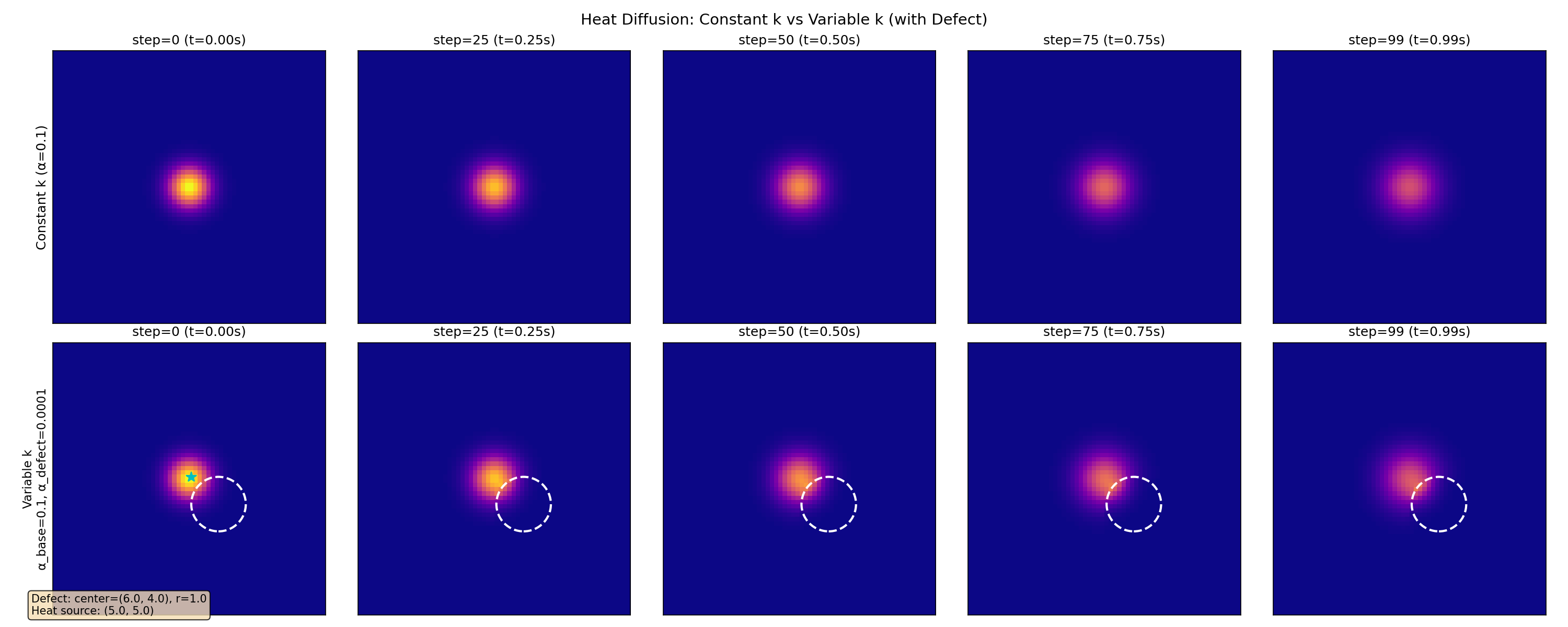
To test spatially varying material properties, we introduce a low-diffusivity spherical defect embedded in a homogeneous background. As illustrated in Fig. 14 (bottom row), the heat propagation is locally impeded near the defect region, resulting in a clearly asymmetric temperature field. This behavior is consistent with the physical interpretation of reduced thermal diffusivity.

F.5 Effect of Diffusivity Magnitude

Figure 15: Surface Temperature Profiles under Different Diffusivities. One-dimensional cross-sections of the surface temperature along the $x$ direction at the midline ($y=\mathrm{middle}$), comparing high diffusivity ($\alpha=1.0$) and low diffusivity ($\alpha=0.1$). (Left) At the initial time step, both cases exhibit identical Gaussian profiles, confirming consistent initialization. (Right) At the final time step, the high-diffusivity case shows a significantly broader and lower-amplitude profile, reflecting faster spatial spreading of heat, while the low-diffusivity case retains a sharper peak. These results qualitatively validate the expected dependence of diffusion dynamics on the thermal diffusivity parameter $\alpha$.

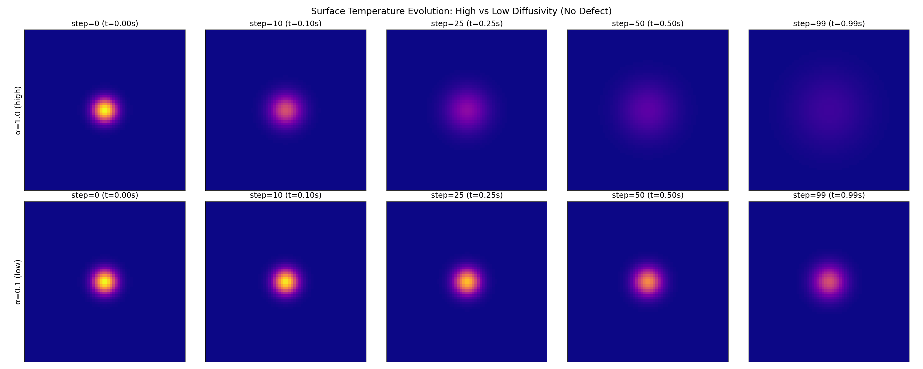
We also compare diffusion dynamics under different diffusivity values in a defect-free setting. Figure 15 contrasts $\alpha=1.0$ (high diffusivity) with $\alpha=0.1$ (low diffusivity) using identical spatial and temporal resolutions. As expected, higher diffusivity leads to significantly faster spreading and lower peak temperatures, while preserving the overall Gaussian structure.

Appendix G Limitations and Future Work

While NeFTY demonstrates significant improvements in quantitative thermal tomography, several limitations inherent to the current formulation present avenues for future research.

Inference Latency and Test-Time Optimization. Unlike end-to-end learning approaches (e.g., U-Net (Ronneberger et al., 2015)) that perform inference in milliseconds, NeFTY relies on test-time optimization. Recovering the diffusivity field for a single specimen requires approximately 10 minutes of iterative optimization on a high-end GPU. This computational cost, while tractable for NDE inspection where accuracy is paramount, currently limits the applicability of the method in high-throughput manufacturing lines requiring real-time feedback. Future work could explore amortized inference techniques, such as meta-learning or hypernetworks, to predict good initialization parameters for the neural field, thereby significantly reducing the number of optimization steps required for convergence.

Numerical Stability and Defect Contrast. As detailed in Appendix D.1, we currently scale the defect-to-bulk diffusivity contrast to approximately 1:20 to maintain the condition number of the linear system. Realistic air voids can exhibit contrast ratios exceeding 1:1000. While our current results demonstrate that the method can resolve geometries despite this scaling, recovering the exact quantitative thermal properties of high-contrast voids remains challenging due to the vanishing gradients inside highly insulating regions. Future iterations of NeFTY could incorporate preconditioning techniques or multi-grid solvers within the differentiable loop to better handle stiff, high-contrast regimes.

Synthetic-to-Real Gap. Our experiments are currently conducted on high-fidelity synthetic data generated by a distinct physics engine (Holl and Thuerey, 2024) to avoid the inverse crime. While this validates the method’s robustness to discretization shifts, real-world experimental data introduces additional complexities such as non-uniform surface emissivity, sensor noise patterns, and non-instantaneous flash heating pulses. Validating NeFTY on datasets collected in the real world is a critical priority for future development.