Redefining shared information: a heterogeneity-adaptive framework for meta-analysis

Abstract

Meta-analytic methods tend to take all-or-nothing approaches to study-level heterogeneity, assuming all studies are heterogeneous or homogeneous, leading to inefficiency and/or bias in estimation and inference. In this paper, we develop a heterogeneity-adaptive meta-analysis in linear models that adapts to the amount of information shared between datasets. The primary mechanism for the information-sharing is a shrinkage of dataset-specific distributions towards a new “centroid” distribution through a Kullback-Leibler divergence penalty. The Kullback-Leibler divergence is uniquely geometrically suited for measuring relative information between datasets, and leads to relatively simple closed form estimators with intuitive interpretations. We establish our estimator’s desirable inferential properties without assuming homogeneity of dataset parameters. Among other results, we show that our estimator has a provably smaller mean squared error than the dataset-specific maximum likelihood estimators, and establish asymptotically valid inference procedures. A comprehensive set of simulations highlights our estimator’s versatility, and an analysis of data from the eICU Collaborative Research Database illustrates its performance in a real-world setting.

Keywords: Data fusion, Information geometry, Linear model, Ridge regression, Stein shrinkage.

1 Introduction

Meta-analyses estimate a single, shared parameter using summary statistics from different studies. Parameter heterogeneity across studies is fundamentally undesirable; in this case, a single unifying parameter may not exist or be interpretable. Prior work has mostly focused on limiting or controlling for heterogeneity. Meta-analyses begin with systematic literature reviews intended to exclude studies that may be measuring different parameters (Pigott and Polanin,, 2020). More recent work accomplishes this exclusion empirically, by down-weighting studies that have a different parameter from a shared parameter of interest (Xie et al.,, 2011; Wang et al.,, 2023; Noma et al.,, 2024). Additional heterogeneity may be incorporated by formally modeling the distribution of study-specific effects, as in random-effects meta-analysis. In random-effects meta-analysis, study parameters are conceptualized as randomly drawn from a population, and the meta-estimator is a function of the variance in the study parameters (Dersimonian and Laird,, 1986). In the absence of a common, shared parameter, these approaches do not provide meaningful inference.

We propose an alternative treatment of heterogeneity in meta-analysis using the linear model, one which shifts the focus from estimating a single, homogeneous parameter to improving estimation of individual study parameters by allowing adaptive information sharing across studies. Our approach requires neither the existence of a shared parameter nor a specified underlying generative model for the study parameters. The primary mechanism for the information-sharing is a shrinkage of study-specific distributions towards a new “centroid” distribution through a Kullback-Leibler divergence (KLD) penalty (Kullback and Leibler,, 1951). This centroid distribution, while not meaningfully interpretable in the presence of heterogeneity, serves a crucial role in linking the individual studies because its estimation introduces additional flexibility into the information-borrowing. Indeed, our formulation jointly estimates parameters of both the unknown study-specific distributions and the centroid distribution. By equipping each study with its own shrinkage parameter and selecting the shrinkage parameters that minimize the mean squared error of the study-specific estimators, our framework borrows information adaptively and efficiently according to heterogeneity in the observed data.

In contrast to more frequently used measures of heterogeneity such as the Euclidean distance between parameters, we use the KLD of the study distributions from the centroid distribution. This difference is important because it accounts not only for differences between the parameters but also for other important features of the data that induce heterogeneity, such as the error and covariate variances. The KLD is the appropriate divergence on the information space, and we argue that it is a more geometrically appropriate quantification of the similarity between study distributions than the more common Euclidean distance. We show that our use of the KLD to quantify the similarity between studies yields relatively simple parameter estimates with desirable and intuitive interpretations. In conjunction with the flexibility of our estimated centroid, this has important consequences for the statistical advantages of our estimator, such as asymptotic bias control and smaller mean squared errors. Notably, we show that our estimator outperforms the study-specific maximum likelihood estimators, in a mean squared error sense, while also yielding asymptotically unbiased inference on the individual study parameters.

This paper is organized as follows. Section 2 chronicles the evolution of meta-analysis and its responses to heterogeneity through to recent developments. Section 3 describes the model, presents a closed form solution for our estimator and develops an intuition for its behavior under different shrinkage parameter settings. In Section 4, we investigate the theoretical properties of our estimator. We show that, similar to a Stein shrinkage result, it is always better in a mean squared error sense to borrow information across studies, even in the presence of substantial heterogeneity. Under mild conditions, we also show that our estimator is consistent and we derive asymptotically valid inference procedures. Section 5 describes the data-driven selection of the amount of information borrowed, and the theoretical “gap” between the optimal information borrowed and its data-driven counterpart. Section 6 examines the performance of our estimator in simulation studies. An analysis of data from the eICU Collaborative Research Database in Section 7 illustrates our estimator’s behavior in a real-life setting. Lengthy derivations, proofs and additional numerical results are deferred to the supplement.

2 Historical evolution of meta-analysis

Meta-analysis became a field for concentrated methodological development in the 1970s. Existing methods for synthesizing studies, including vote counting, proved insufficient to handle the growing body of research findings in education and psychology (Shadish and Lecy,, 2015). Glass, (1976), coining the term meta-analysis, advocated for the development of systematic practices to synthesize findings from primary studies and proposed averaging standardized effect sizes to estimate an underlying parameter of interest. Earlier work by Cochran, (1954) in the context of agricultural experiments similarly proposed taking a weighted average of estimates, using the inverse of a study estimate’s standard error as the weight. Becker and Wu, (2007) expanded this procedure to multiple linear regression parameters. While this fixed-effect meta-estimator is the best linear unbiased estimator when all study parameters are equal, the most prevalent critique is that it may include studies measuring different parameters, leading to misinterpretation of the meta-estimate (Eysenck,, 1978; Rice et al.,, 2018; Hector et al.,, 2024; Gurevitch et al.,, 2018).

The random-effects meta-analysis model was an early response to concerns of parameter heterogeneity and became one of the primary approaches to meta-analysis (Hedges,, 1983; Dersimonian and Laird,, 1986). This approach views the study-specific parameters as sampled from a distribution centered around a shared parameter of interest. Then, the heterogeneity of the study parameters is due solely to this sampling mechanism and is incorporated into estimation of the shared parameter through random study effects. One limitation to this approach is that it often assumes that the study parameters are normally distributed about the shared parameter, an assumption that often does not hold in practice (Liu et al.,, 2023). Bayesian approaches consider other underlying distributions (Lee and Thompson,, 2008; Noma et al.,, 2022) but the issue remains of identifying a suitable distribution for the random effects. Frequentist approaches have focused on consistent meta-estimation in the presence of outliers and individual studies that violate normality. For example, Noma et al., (2024) estimate a shared effect by minimizing the density power divergence, which can be less sensitive to outliers than fixed- or random-effects methods. The fusion-extraction method proposed by Wang et al., (2023) assumes a critical mass of included studies estimate a single parameter of interest; inconsistent study-specific estimators for that parameter are down-weighted. Similarly, Xie et al., (2011) proposes a confidence distribution-based method that leverages the central limit theorem to allow inference on a shared parameter when the majority of studies are drawn from the population of interest. In the multivariate context, Liu et al., (2015) develop a method to combine confidence densities from different studies, but this technique requires that heterogeneity can be effectively ignored by transforming the heterogeneous parameter to a homogeneous one through known link functions.

Each of these methods focuses on preserving what we term general inference: estimators target parameters for the population of studies from which the selected studies are assumed to be randomly drawn. General inference approaches require an underlying model linking the study parameters to an overarching common parameter of interest. In contrast, a newer approach to handling heterogeneity relies on what we term limited inference. Limited inference does not assume a distributional model for the study-specific parameters, and consequently, inference is limited to the populations represented by the included studies. For example, a limited inference approach proposed by Xie et al., (2011) allows for inference on the median of the study-specific parameters. Claggett et al., (2014) extends this method by connecting confidence distributions with bootstrap sampling to conduct inference on the ordered set of study-specific parameters.

Existing meta-analytic methods face a trade-off: either they require strong assumptions about the structure of the heterogeneity, or their inference is generalizable only to the study populations. Recent work in transfer learning from Hector and Martin, (2024) suggests a mechanism to calibrate the generality of inference according to the amount of heterogeneity by allowing partial borrowing based on a data-driven quantification of heterogeneity. They propose an “information-based regularization” where a target study estimate borrows differentially from a source estimate depending on the magnitude of the KLD from the source likelihood. This differential information borrowing does not require prespecifying a model that links the parameters of the two studies. By introducing a controlled amount of bias, Hector and Martin, (2024) show that the optimal estimator (in a mean squared error sense) should always incorporate some information from the external study, even in the presence of unstructured heterogeneity.

On the one hand, this result is promising because it suggests that some information borrowing may be useful in the meta-analysis context, even in the presence of heterogeneity. On the other hand, the existence of a similar result for meta-analysis is not obvious. The transfer learning goal is a fundamentally asymmetric inference focusing on a target study, while meta-analysis considers inference on all studies. Our introduction of a “centroid” distribution becomes crucial for linking the individual studies because it adapts to this asymmetry by effectively introducing a “source” distribution. The main difference between our centroid and a source distribution, however, is that the centroid is not fixed but rather needs to be estimated. This fundamental difference leads to both additional complications and intuitive and desirable interpretations. For example, as we will show in the next section, in some settings this estimated centroid yields the fixed-effect meta-estimator.

3 The heterogeneity-adaptive estimator

3.1 Estimation with common covariates

Consider a scenario with $k$ independent studies, indexed $j=1,\dots,k$, where each study collects $n_{j}$ observations consisting of an outcome vector $\boldsymbol{Y}_{j}\in\mathbb{R}^{n_{j}}$ and a matrix of covariates $\boldsymbol{X}_{j}\in\mathbb{R}^{n_{j}\times p}$. We assume the covariates are associated with the outcomes in each study through the model $\boldsymbol{Y}_{j}\sim\mathcal{N}(\boldsymbol{X}_{j}\boldsymbol{\beta}_{j},\sigma_{j}^{2}\boldsymbol{I}_{n_{j}})$, with $\boldsymbol{I}_{n_{j}}$ the $n_{j}\times n_{j}$ identity matrix. Let $\boldsymbol{X}=\text{block-diag}\{\boldsymbol{X}_{1},\ldots,\boldsymbol{X}_{k}\}$ be the block-diagonal assembly of covariate matrices $\boldsymbol{X}_{j}$ with dimension $\sum_{j=1}^{k}n_{j}\times pk$ and $\boldsymbol{Y}=(\boldsymbol{Y}_{1},\ldots,\boldsymbol{Y}_{k})$ be the outcome vectors appended in the same order. Then, the joint model for all $k$ studies is

$$\boldsymbol{Y}=\boldsymbol{X}\boldsymbol{\beta}+\boldsymbol{\epsilon},\quad\boldsymbol{\epsilon}\sim\mathcal{N}(\boldsymbol{0},\boldsymbol{\Sigma}),$$

where $\boldsymbol{\Sigma}=\text{block-diag}\{\sigma^{2}_{1}\boldsymbol{I}_{n_{1}},\ldots,\sigma^{2}_{k}\boldsymbol{I}_{n_{k}}\}$ is the block-diagonal matrix of dataset-specific variances and $\boldsymbol{\beta}=(\boldsymbol{\beta}_{1},\ldots,\boldsymbol{\beta}_{k})\in\mathbb{R}^{pk}$. Estimating $\boldsymbol{\beta}$ using maximum likelihood estimation returns a stacked vector of the maximum likelihood estimators (MLEs) for the individual datasets, $\boldsymbol{\tilde{\beta}}=(\boldsymbol{\tilde{\beta}}_{1},\dots,\boldsymbol{\tilde{\beta}}_{k})^{\prime}$, without any information shared between them; modeling in this way treats $\boldsymbol{\beta}_{j}$ and $\boldsymbol{\beta}_{j^{\prime}}$ for any studies $j$ and $j^{\prime}$ as though there is complete heterogeneity. In contrast, if we believe it is reasonable to assume perfect homogeneity so that $\boldsymbol{\beta}_{j}=\boldsymbol{\beta}_{j^{\prime}}$ for all $j,j^{\prime}\in\{1,\dots,k\}$, the MLE is the uniformly minimum variance unbiased estimator used in fixed-effects meta-analysis,

$$\boldsymbol{\tilde{\beta}}_{\textsf{FE}} =(\boldsymbol{X}^{\top}\boldsymbol{\Sigma}^{-1}\boldsymbol{X})^{-1}\boldsymbol{X}^{\top}\boldsymbol{\Sigma}^{-1}\boldsymbol{Y}=(\boldsymbol{X}^{\top}\boldsymbol{\Sigma}^{-1}\boldsymbol{X})^{-1}\boldsymbol{X}^{\top}\boldsymbol{\Sigma}^{-1}\boldsymbol{X}\boldsymbol{\tilde{\beta}}.$$ (1)

Clearly, there is a homogeneity/heterogeneity continuum between the assumptions that $\boldsymbol{\beta}_{j}\neq\boldsymbol{\beta}_{j^{\prime}}$ for all $j\neq j^{\prime}$ and $\boldsymbol{\beta}_{j}=\boldsymbol{\beta}_{j^{\prime}}$ for all $j\neq j^{\prime}$ that is not captured by $\boldsymbol{\tilde{\beta}}$ or $\boldsymbol{\tilde{\beta}}_{\textsf{FE}}$. Further, the ends of the spectrum, i.e. the full homogeneity and full heterogeneity assumptions, treat all studies equally by assuming the same level of heterogeneity (no or full heterogeneity) for all parameters. In contrast, we propose an estimator for $\boldsymbol{\beta}$ along the homogeneity/heterogeneity continuum that is fully adaptive in the sense that each study may be more or less heterogeneous than the others.

First, we encourage information-sharing between studies by shrinking estimates for $\boldsymbol{\beta}_{j}$ from outcome distributions that are “far” from the other studies. We begin by defining a “centroid” outcome distribution for study $j$, $\mathcal{N}(\boldsymbol{X}_{j}\boldsymbol{\theta},\sigma_{j}^{2}\boldsymbol{I})$, where $\boldsymbol{\theta}\in\mathbb{R}^{p}$. As an algebraic simplification, the centroid distribution’s variance is allowed to vary with dataset $j$. To measure the difference between using $\mathcal{N}(\boldsymbol{X}_{j}\boldsymbol{\theta},\sigma_{j}^{2}\boldsymbol{I}_{n_{j}})$ and $\mathcal{N}(\boldsymbol{X}_{j}\boldsymbol{\beta}_{j},\sigma_{j}^{2}\boldsymbol{I}_{n_{j}})$ to model $\boldsymbol{Y}_{j}$, we seek a topologically appropriate measure that, in contrast to the Euclidean distance between parameters, accounts for other features of the distributions, such as the error and covariate variances. To compare the distributions, we use the Kullback-Leibler divergence (KLD) (Amari,, 2020; Kullback and Leibler,, 1951). The KLD is the unique Bregman divergence on the manifold of Gaussian distributions, and it measures the relative entropy of a distribution $\mathcal{N}(\boldsymbol{X}_{j}\boldsymbol{\beta}_{j},\sigma_{j}^{2}\boldsymbol{I}_{n_{j}})$ with respect to another distribution $\mathcal{N}(\boldsymbol{X}_{j}\boldsymbol{\theta},\sigma_{j}^{2}\boldsymbol{I}_{n_{j}})$. It also measures the excess surprise from using $\mathcal{N}(\boldsymbol{X}_{j}\boldsymbol{\theta},\sigma_{j}^{2}\boldsymbol{I}_{n_{j}})$ over $\mathcal{N}(\boldsymbol{X}_{j}\boldsymbol{\beta}_{j},\sigma_{j}^{2}\boldsymbol{I}_{n_{j}})$, when $\mathcal{N}(\boldsymbol{X}_{j}\boldsymbol{\beta}_{j},\sigma_{j}^{2}\boldsymbol{I}_{n_{j}})$ is the true distribution. Since a manifold is locally equivalent to a Euclidean space, small divergences between the distributions are equivalent to small distances between the parameters themselves. This deformation only holds locally, however, so that large divergences between $\mathcal{N}(\boldsymbol{X}_{j}\boldsymbol{\theta},\sigma_{j}^{2}\boldsymbol{I}_{n_{j}})$ and $\mathcal{N}(\boldsymbol{X}_{j}\boldsymbol{\beta}_{j},\sigma_{j}^{2}\boldsymbol{I}_{n_{j}})$ do not necessarily equate to large distances between $\boldsymbol{\theta}$ and $\boldsymbol{\beta}_{j}$.

To estimate $\boldsymbol{\beta}$, we maximize the joint log-likelihood subject to the constraint that all study-specific distributions be close in relative entropy to the centroid distribution, or equivalently

$$O(\boldsymbol{Y},\boldsymbol{X};\boldsymbol{\beta},\boldsymbol{\theta},\boldsymbol{\sigma}^{2})=\sum_{j=1}^{k}\Bigl\{-\frac{1}{2\sigma^{2}_{j}}\|\boldsymbol{Y}_{j}-\boldsymbol{X}_{j}\boldsymbol{\beta}_{j}\|^{2}-\Bigl(\frac{\pi_{j}}{1-\pi_{j}}\Bigr)\Bigl(\frac{1}{2\sigma_{j}^{2}}\Bigr)\|\boldsymbol{X}_{j}\boldsymbol{\beta}_{j}-\boldsymbol{X}_{j}\boldsymbol{\theta}\|^{2}\Bigr\},$$ (2)

where the shrinkage parameter for each study is $\pi_{j}/(1-\pi_{j})$, $\pi_{j}\in[0,1]$. At $\pi_{j}=1$, the penalty is infinite and the estimate for $\boldsymbol{\beta}_{j}$ is required to equal the estimate for $\boldsymbol{\theta}$. For simplicity of exposition, we treat $\sigma_{j}^{2}$ as known in all derivations; in practice, we estimate it using its MLE from study $j$. Define $\boldsymbol{\pi}=(\pi_{1},\dots,\pi_{k})^{\prime}$, the vector of shrinkage parameters. We give the closed-form estimators that maximize $O(\boldsymbol{Y},\boldsymbol{X};\boldsymbol{\beta},\boldsymbol{\theta},\boldsymbol{\sigma}^{2})$ below, with the non-trivial derivations relegated to Section A of the supplement. The centroid that maximizes this objective function is

$$\boldsymbol{\widehat{\theta}}(\boldsymbol{\pi}) =\Bigl(\sum_{j=1}^{k}\frac{\pi_{j}}{\sigma_{j}^{2}}\boldsymbol{X}_{j}^{\prime}\boldsymbol{X}_{j}\Bigr)^{-1}\sum_{j=1}^{k}\frac{\pi_{j}}{\sigma_{j}^{2}}\boldsymbol{X}_{j}^{\prime}\boldsymbol{Y}_{j}=\Bigl(\sum_{j=1}^{k}\frac{\pi_{j}}{\sigma_{j}^{2}}\boldsymbol{X}_{j}^{\prime}\boldsymbol{X}_{j}\Bigr)^{-1}\sum_{j=1}^{k}\frac{\pi_{j}}{\sigma_{j}^{2}}\boldsymbol{X}_{j}^{\prime}\boldsymbol{X}_{j}\boldsymbol{\tilde{\beta}}_{j},$$ (3)

and study $j$’s estimator for $\boldsymbol{\beta}_{j}$, $\boldsymbol{\widehat{\beta}}_{j}(\boldsymbol{\pi})$, can be written as a convex combination of the MLE, $\boldsymbol{\tilde{\beta}}_{j}$, and the centroid estimator:

$$\boldsymbol{\widehat{\beta}}_{j}(\boldsymbol{\pi}) =(1-\pi_{j})\boldsymbol{\tilde{\beta}}_{j}+\pi_{j}\boldsymbol{\widehat{\theta}}(\boldsymbol{\pi}).$$ (4)

The full vector of $\boldsymbol{\widehat{\beta}}(\boldsymbol{\pi})=\{\boldsymbol{\widehat{\beta}}_{1}(\boldsymbol{\pi})^{\prime},\dots,\boldsymbol{\widehat{\beta}}_{k}(\boldsymbol{\pi})^{\prime}\}^{\prime}$ is

$$\boldsymbol{\widehat{\beta}}(\boldsymbol{\pi}) =(\boldsymbol{I}_{pk}-\boldsymbol{\Pi})\boldsymbol{\tilde{\beta}}+\boldsymbol{\Pi}\boldsymbol{K}\boldsymbol{\widehat{\theta}}(\boldsymbol{\pi})=\boldsymbol{\tilde{\beta}}+\boldsymbol{\Pi}\{\boldsymbol{K}\boldsymbol{A}(\boldsymbol{\pi})-\boldsymbol{I}_{pk}\}\boldsymbol{\tilde{\beta}},$$ (5)

where $\boldsymbol{K}=\boldsymbol{1}_{k}\otimes\boldsymbol{I}_{p}$ is a matrix which stacks the vector to its right with $\otimes$ the Kronecker product, $\boldsymbol{\Pi}=\text{block-diag}\{\pi_{j}\boldsymbol{I}_{p}\}\in\mathbb{R}^{pk\times pk}$, and $\boldsymbol{A}(\boldsymbol{\pi})=(\boldsymbol{K}^{\prime}\boldsymbol{\Pi}\boldsymbol{X}^{\top}\boldsymbol{\Sigma}^{-1}\boldsymbol{X}\boldsymbol{K})^{-1}\boldsymbol{K}^{\prime}\boldsymbol{\Pi}\boldsymbol{X}^{\top}\boldsymbol{\Sigma}^{-1}\boldsymbol{X}$.

Both $\boldsymbol{\widehat{\beta}}(\boldsymbol{\pi})$ and $\boldsymbol{\widehat{\theta}}(\boldsymbol{\pi})$ are extremely flexible because they shift with the choice of shrinkage parameter $\boldsymbol{\pi}$. The dependence of $\boldsymbol{\widehat{\theta}}(\boldsymbol{\pi})$ on the shrinkage parameters $\boldsymbol{\pi}$ makes the centroid capable of representing the space of heterogeneity patterns. This includes representation of some recognizable meta-estimators. When $\pi_{j}=\pi_{j^{\prime}}$ for all $j\neq j^{\prime}$, $\boldsymbol{\widehat{\theta}}(\boldsymbol{\pi})=\boldsymbol{\tilde{\beta}}_{\textsf{FE}}$ the fixed-effect meta-estimator in equation (1). If $\boldsymbol{\pi}$ is zero for $k-x$ studies and non-zero and equal for the remaining $x$ studies ($x\in\mathbb{Z},0\leq x\leq k$), then $\boldsymbol{\widehat{\theta}}(\boldsymbol{\pi})$ is the fixed-effect meta-estimator for the studies with non-zero $\pi_{j}$. If $\boldsymbol{\pi}$ contains zeroes for all studies except the $j$^th, then $\boldsymbol{\widehat{\theta}}(\boldsymbol{\pi})=\boldsymbol{\tilde{\beta}}_{j}$. Panel A in Figure 1 shows the possible values of $\boldsymbol{\widehat{\theta}}(\boldsymbol{\pi})$ given the maximum likelihood estimates $\boldsymbol{\tilde{\beta}}_{j}$ and information matrices for four studies with $p=2$ covariates.

The estimates $\boldsymbol{\widehat{\beta}}_{j}(\boldsymbol{\pi})$ for the study-specific parameters also depend on $\boldsymbol{\pi}$. Panels B and C of Figure 1 show the set of feasible estimates $\boldsymbol{\widehat{\beta}}(\boldsymbol{\pi})$ for the same data as displayed in panel A, with examples for changes in $\boldsymbol{\pi}$. Each corner is the MLE for a particular study. In panel B, we see that a move from $\boldsymbol{\pi}=(0.2,0.2,0.2,0.2)$ to $\boldsymbol{\pi}=(0.8,0.8,0.8,0.8)$ pulls all estimates for $\boldsymbol{\widehat{\beta}}_{j}(\boldsymbol{\pi})$ towards the fixed-effect meta-estimator $\boldsymbol{\tilde{\beta}}_{\textsf{FE}}$. In panel C, which displays a move from $\boldsymbol{\pi}=(0.5,0.5,0.5,0)$ to $\boldsymbol{\pi}=(0.5,0.5,0.5,0.3)$, an increase in the contribution from study 4 shifts the estimates for studies 1, 2, and 3 towards $\boldsymbol{\tilde{\beta}}_{4}$. We aim to select $\boldsymbol{\pi}$ to minimize the mean squared error (MSE) of $\boldsymbol{\widehat{\beta}}(\boldsymbol{\pi})$, which we discuss further in Section 4.

Figure 1: Panel A displays possible values for $\boldsymbol{\widehat{\theta}}(\boldsymbol{\pi})$ for four datasets. Any coordinate pair within the outlined shape can be obtained for an appropriate $\boldsymbol{\pi}$ vector. Panels B and C display possible values for each $\boldsymbol{\widehat{\beta}}_{j}(\boldsymbol{\pi})$ for $k=4$. For a given dataset, denoted by color, any coordinate pair within the polygon may be obtained for an appropriate $\boldsymbol{\pi}$ vector. In example A, arrows display a shift from $\boldsymbol{\pi}=(0.2,0.2,0.2,0.2)$ to $\boldsymbol{\pi}=(0.8,0.8,0.8,0.8)$. In example B, arrows display a shift from $\boldsymbol{\pi}=(0.5,0.0,0.5,0.5)$ to $\boldsymbol{\pi}=(0.5,0.5,0.5,0.3)$.

Our objective function is equivalent to a penalized seemingly unrelated regression (Zellner,, 1962). Prior work on Stein shrinkage in seemingly unrelated regression by Mehrabani and Ullah, (2020) takes a weighted average of the fixed-effect meta-estimator $\boldsymbol{\tilde{\beta}}_{\textsf{FE}}$ and the individual study MLEs $\boldsymbol{\tilde{\beta}}_{j}$. The new insight afforded by our formulation shows that the weighted average proposed in Mehrabani and Ullah, (2020) maximizes our objective function in equation (2) when $\pi_{j}\equiv\pi$. Our formulation, however, not only allows each study to have its own weight, as shown in equation (4), but also incorporates alternative patterns of heterogeneity beyond the fixed-effect meta-estimator. Further, by selecting our weights to minimize the MSE, we show in Section 4 that our framework enables asymptotically valid inference, a property absent in Mehrabani and Ullah, (2020).

3.2 Estimation with overlapping covariates

In Section 3.1, we assumed that the same covariates are measured across the $k$ datasets, which may not always be the case in practice. Consider instead the setting where the $j$th study has $q_{j}\geq p$ covariates, $p$ of which are common across studies. The remaining $q_{j}-p$ covariates may be measuring different features. This captures a common structure of univariate meta-analyses: each study may control for different covariates, and the standardized effect sizes for a main effect of interest are combined.

For study $j$, denote the $n_{j}\times p$ matrix for the effects of interest as $\boldsymbol{X}_{j}$ and denote the $n_{j}\times(q_{j}-p)$ matrix of control covariates as $\boldsymbol{Z}_{j}$. Outcomes for study $j$ are modeled as

$$\boldsymbol{Y}_{j}=\boldsymbol{X}_{j}\boldsymbol{\beta}_{j}+\boldsymbol{Z}_{j}\boldsymbol{\gamma}_{j}+\epsilon_{j},\quad\epsilon_{j}\sim N(\boldsymbol{0},\sigma_{j}^{2}\boldsymbol{I}_{n_{j}}).$$ (6)

Our goal is to estimate $\boldsymbol{\beta}=(\boldsymbol{\beta}_{1},\ldots,\boldsymbol{\beta}_{k})$ in the framework proposed in Section 3.1. Assume study $j$ reports the maximum likelihood estimators $\boldsymbol{\tilde{\beta}}_{j}$ and $\boldsymbol{\tilde{\gamma}}_{j}$ for $\boldsymbol{\beta}_{j}$ and $\boldsymbol{\gamma}_{j}$, respectively, and the covariance matrix for the estimators,

$$\sigma^{2}_{j}\begin{bmatrix}\boldsymbol{X}_{j}^{\top}\boldsymbol{X}_{j}&\boldsymbol{X}_{j}^{\top}\boldsymbol{Z}_{j}\\ \boldsymbol{Z}_{j}^{\top}\boldsymbol{X}_{j}&\boldsymbol{Z}_{j}^{\top}\boldsymbol{Z}_{j}\end{bmatrix}^{-1}.$$ (7)

To reformulate equation (6) with only the covariates in common across datasets, we first project the outcome model onto the null space of $\boldsymbol{Z}_{j}$. Let $\boldsymbol{M}_{j}=\boldsymbol{I}_{n_{j}}-\boldsymbol{Z}_{j}(\boldsymbol{Z}_{j}^{\top}\boldsymbol{Z}_{j})^{-1}\boldsymbol{Z}_{j}^{\top}$ when $q_{j}>p$, and $\boldsymbol{M}_{j}=\boldsymbol{I}_{n_{j}}$ when $q_{j}=p$. In this projected outcome model, additional covariates $\boldsymbol{Z}_{j}$ are removed:

$$\boldsymbol{M}_{j}\boldsymbol{Y}_{j}=\boldsymbol{M}_{j}\boldsymbol{X}_{j}\boldsymbol{\beta}_{j}+\boldsymbol{M}_{j}\epsilon_{j},\quad\boldsymbol{M}_{j}\epsilon_{j}\sim N(\boldsymbol{0},\sigma_{j}^{2}\boldsymbol{M}_{j}).$$ (8)

Given the outcome model in equation (8), the objective function in equation (2) becomes

$$\sum_{j=1}^{k}\Bigl\{-\frac{1}{2\sigma^{2}_{j}}(\boldsymbol{M}_{j}\boldsymbol{Y}_{j}-\boldsymbol{M}_{j}\boldsymbol{X}_{j}\boldsymbol{\beta}_{j})^{\top}\boldsymbol{M}_{j}^{+}(\boldsymbol{M}_{j}\boldsymbol{Y}_{j}-\boldsymbol{M}_{j}\boldsymbol{X}_{j}\boldsymbol{\beta}_{j})$$

$$\quad-\Bigl(\frac{\pi_{j}}{1-\pi_{j}}\Bigr)\Bigl(\frac{1}{2\sigma_{j}^{2}}\Bigr)(\boldsymbol{M}_{j}\boldsymbol{X}_{j}\boldsymbol{\beta}_{j}-\boldsymbol{M}_{j}\boldsymbol{X}_{j}\boldsymbol{\theta})^{\top}\boldsymbol{M}_{j}^{+}(\boldsymbol{M}_{j}\boldsymbol{X}_{j}\boldsymbol{\beta}_{j}-\boldsymbol{M}_{j}\boldsymbol{X}_{j}\boldsymbol{\theta})\Bigr\},$$ (9)

where $\boldsymbol{M}_{j}^{+}$ is the generalized inverse of $\boldsymbol{M}_{j}$; as $\boldsymbol{M}_{j}$ is idempotent, it only has an inverse when $\boldsymbol{M}_{j}=\boldsymbol{I}_{n_{j}}$. In the objective function in equation (3.2), the KLD penalty shrinks $\boldsymbol{\beta}_{j}$ towards the centroid for the distribution of $\boldsymbol{M}_{j}\boldsymbol{Y}_{j}$. We derive maximizers $\boldsymbol{\widehat{\theta}}_{s}(\boldsymbol{\pi})$ and $\boldsymbol{\widehat{\beta}}_{s}(\boldsymbol{\pi})$ of equation (3.2) in Section A of the supplement, and give their closed forms here:

$$\boldsymbol{\widehat{\theta}}_{s}(\boldsymbol{\pi}) =\Bigl(\sum_{j=1}^{k}\frac{\pi_{j}}{\sigma_{j}^{2}}\boldsymbol{X}_{j}^{\prime}\boldsymbol{M}_{j}\boldsymbol{X}_{j}\Bigr)^{-1}\sum_{j=1}^{k}\frac{\pi_{j}}{\sigma_{j}^{2}}\boldsymbol{X}_{j}^{\prime}\boldsymbol{M}_{j}\boldsymbol{X}_{j}\boldsymbol{\tilde{\beta}}_{j},\quad\boldsymbol{\widehat{\beta}}_{s}(\boldsymbol{\pi})=(\boldsymbol{I}-\boldsymbol{\Pi})\boldsymbol{\tilde{\beta}}+\boldsymbol{\Pi}\boldsymbol{K}\boldsymbol{\widehat{\theta}}_{s}(\boldsymbol{\pi}),$$

where $\boldsymbol{M}=\text{block-diag}\{\boldsymbol{M}_{1},\ldots,\boldsymbol{M}_{k}\}$. Provided we have access to the full covariance matrix in equation (7), we can compute $\boldsymbol{X}_{j}^{\top}\boldsymbol{M}_{j}\boldsymbol{X}_{j}$ following

$$\boldsymbol{X}_{j}^{\top}\boldsymbol{M}_{j}\boldsymbol{X}_{j} =\boldsymbol{X}_{j}^{\top}\{\boldsymbol{I}-\boldsymbol{Z}_{j}(\boldsymbol{Z}_{j}^{\top}\boldsymbol{Z}_{j})^{-1}\boldsymbol{Z}_{j}^{\top}\}\boldsymbol{X}_{j}=\boldsymbol{X}_{j}^{\top}\boldsymbol{X}_{j}-\boldsymbol{X}_{j}^{\top}\boldsymbol{Z}_{j}(\boldsymbol{Z}_{j}^{\top}\boldsymbol{Z}_{j})^{-1}\boldsymbol{Z}_{j}^{\top}\boldsymbol{X}_{j}.$$

When covariates $\boldsymbol{Z}_{j}$ are orthogonal to $\boldsymbol{X}_{j}$ for all $j=1,\ldots,k$, the above estimators simplify to those from Section 3.1: $\boldsymbol{\widehat{\theta}}_{s}(\boldsymbol{\pi})=\boldsymbol{\widehat{\theta}}(\boldsymbol{\pi})$ and $\boldsymbol{\widehat{\beta}}_{s}(\boldsymbol{\pi})=\boldsymbol{\widehat{\beta}}(\boldsymbol{\pi})$.

4 Theoretical support

For simplicity of exposition, we focus on deriving theoretical support for the estimators in Section 3.1; similar results can be shown for those in Section 3.2 and are omitted. Our goal is to improve estimation across all studies on average by selecting the shrinkage parameter vector $\boldsymbol{\pi}$ that minimizes the mean squared error of $\boldsymbol{\widehat{\beta}}(\boldsymbol{\pi})$. The MSE-minimizing $\boldsymbol{\pi}$ balances both variance and bias of our estimator and, hopefully, leads to an improvement over the MLE, $\boldsymbol{\tilde{\beta}}$. We begin by demonstrating that such an improvement exists using the simplified setting where $\pi_{j}\equiv\pi$. We subsequently extend our results to general $\boldsymbol{\pi}$ vectors by developing an alternative parameterization that yields an interpretable closed-form solution for the optimal scale of borrowing between datasets. Finally, we show that our estimator is consistent and asymptotically normal at the optimal scaling, enabling asymptotically valid inference.

Our objective is to select $\boldsymbol{\pi}$ to minimize the MSE of $\boldsymbol{\widehat{\beta}}(\boldsymbol{\pi})$, derived in Section B of the supplement and given by

$$\mathsf{MSE}\{\boldsymbol{\widehat{\beta}}(\boldsymbol{\pi})\} =\|\boldsymbol{\Pi}\{\boldsymbol{K}\boldsymbol{A}(\boldsymbol{\pi})-\boldsymbol{I}_{pk}\}\boldsymbol{\beta}\|^{2}+\mathsf{tr}(\mathsf{Var}[\boldsymbol{\Pi}\{\boldsymbol{K}\boldsymbol{A}(\boldsymbol{\pi})-\boldsymbol{I}_{pk}\}\boldsymbol{\tilde{\beta}}])$$

$$\quad+2\mathsf{tr}(\mathsf{Cov}[\boldsymbol{\tilde{\beta}},\boldsymbol{\Pi}\{\boldsymbol{K}\boldsymbol{A}(\boldsymbol{\pi})-\boldsymbol{I}_{pk}\}\boldsymbol{\tilde{\beta}}])+\mathsf{tr}\{\mathsf{Var}(\boldsymbol{\tilde{\beta}})\},$$ (10)

where $\mathsf{tr}(\cdot)$ denotes the trace of a matrix. A preliminary question is whether minimizing this MSE leads to a choice of $\boldsymbol{\pi}$ that necessarily offers an improvement, in mean squared error, over using the study-specific MLEs. To see that it does, we consider a simpler case where all $\pi_{j}\equiv\pi$. If an improvement in MSE exists for this simpler case, then selecting $\boldsymbol{\pi}$ to minimize equation (4) over the full space $[0,1]^{k}$ must yield an estimator $\boldsymbol{\widehat{\beta}}(\boldsymbol{\pi})$ with smaller MSE than the MLE. Theorem 1 states this result formally: there exists a vector $\boldsymbol{\pi}$, $\pi_{j}$ not all zero, such that the MSE of $\boldsymbol{\widehat{\beta}}(\boldsymbol{\pi})$ is strictly less than the MSE of $\boldsymbol{\tilde{\beta}}$, the vector of study-specific MLEs.

Theorem 1.

There exists a $\boldsymbol{\pi}\neq\boldsymbol{0}$ such that $\mathsf{MSE}\{\boldsymbol{\widehat{\beta}}(\boldsymbol{\pi})\}<\mathsf{MSE}(\boldsymbol{\tilde{\beta}}).$ In the case where $\pi_{j}\equiv\pi$, the MSE-minimizing $\pi$ is

$$\pi^{\star} =\frac{-\mathsf{tr}\{(\boldsymbol{K}\boldsymbol{A}-\boldsymbol{I}_{pk})(\boldsymbol{X}^{\top}\boldsymbol{\Sigma}^{-1}\boldsymbol{X})^{-1}\}}{\mathsf{tr}\{(\boldsymbol{K}\boldsymbol{A}-\boldsymbol{I}_{pk})(\boldsymbol{X}^{\top}\boldsymbol{\Sigma}^{-1}\boldsymbol{X})^{-1}(\boldsymbol{K}\boldsymbol{A}-\boldsymbol{I}_{pk})^{\prime}\}+\|(\boldsymbol{K}\boldsymbol{A}-\boldsymbol{I}_{pk})\boldsymbol{\beta}\|^{2}},$$

where $\boldsymbol{A}=(\boldsymbol{K}^{\prime}\boldsymbol{X}^{\top}\boldsymbol{\Sigma}^{-1}\boldsymbol{X}\boldsymbol{K})^{-1}\boldsymbol{K}^{\prime}\boldsymbol{X}^{\top}\boldsymbol{\Sigma}^{-1}\boldsymbol{X}$.

As discussed in Section 3, when $\pi_{j}\equiv\pi$, $\boldsymbol{\widehat{\theta}}(\boldsymbol{\pi})$ is no longer a function of $\boldsymbol{\pi}$ and is equal to the fixed-effect meta-estimator displayed in equation (1). Consequently, $\pi$ can be interpreted as the proportion of $\boldsymbol{\widehat{\beta}}_{j}(\pi)$ coming from the fixed-effect meta-estimator:

$$\boldsymbol{\widehat{\beta}}_{j}(\pi)=(1-\pi)\boldsymbol{\tilde{\beta}}+\pi\boldsymbol{\widehat{\theta}}=\boldsymbol{\tilde{\beta}}+\pi(\boldsymbol{K}\boldsymbol{A}-\boldsymbol{I}_{pk})\boldsymbol{\tilde{\beta}}.$$

When $\pi=0$, $\boldsymbol{\widehat{\beta}}_{j}(0)=\boldsymbol{\tilde{\beta}}$ and the estimator is unbiased. As $\pi$ increases to 1, estimation of $\boldsymbol{\widehat{\beta}}_{j}(\pi)$ leverages more information from the other studies, and the variance of $\boldsymbol{\widehat{\beta}}_{j}(\pi)$ decreases while the bias increases. The proof of Theorem 1 shows further that the bias does not increase too rapidly relative to the variance’s decrease, implying that a range of $\pi$ exists for which the MSE of $\boldsymbol{\widehat{\beta}}(\boldsymbol{\pi})$ is less than that of the MLE. In fact, any $\pi\in(0,2\pi^{\star})$ yields an estimator $\boldsymbol{\widehat{\beta}}(\pi)$ with smaller MSE than the MLE. Mathematical details are given in Section C of the supplement. In our implementation, we use the closed form of $\pi^{\star}$ in Theorem 1 as a starting value when searching for the optimal $\boldsymbol{\pi}$ vector by plugging $\boldsymbol{\tilde{\beta}}$ in for the unknown $\boldsymbol{\beta}$.

Theorem 1 shows that there exists a $\boldsymbol{\pi}$ such that our estimator offers a smaller MSE than the MLE, but it does not provide guidance on how to choose the optimal $\boldsymbol{\pi}$. We next develop a reparameterization of our estimator that decouples the role of $\boldsymbol{\pi}$ in selecting both the centroid and the amount of shrinkage towards the centroid. While technically involved, the reparameterization delivers a closed-form solution for the optimal amount of information borrowing. With this solution, we will be able to show that our estimator is consistent and asymptotically normal under mild conditions.

We motivate the reparameterization in Figure 2 using an example with $k=2$ studies. This figure shows that each pair of $\boldsymbol{\pi}$ values along a ray from the origin gives the same $\boldsymbol{\widehat{\theta}}(\boldsymbol{\pi})$. Mathematically, this is due to the fact that, through a simple rescaling,

$$\boldsymbol{\widehat{\theta}}(\boldsymbol{\pi}) =\Bigl(\sum_{j=1}^{k}\pi_{j}\frac{1}{\sigma_{j}^{2}}\boldsymbol{X}_{j}^{\top}\boldsymbol{X}_{j})^{-1}\sum_{j=1}^{k}\pi_{j}\frac{1}{\sigma_{j}^{2}}\boldsymbol{X}_{j}^{\top}\boldsymbol{X}_{j}\boldsymbol{\tilde{\beta}}=\Bigl(\sum_{j=1}^{k}a\pi_{j}\frac{1}{\sigma_{j}^{2}}\boldsymbol{X}_{j}^{\top}\boldsymbol{X}_{j})^{-1}\sum_{j=1}^{k}a\pi_{j}\frac{1}{\sigma_{j}^{2}}\boldsymbol{X}_{j}^{\top}\boldsymbol{X}_{j}\boldsymbol{\tilde{\beta}}$$

$$=\boldsymbol{\widehat{\theta}}(a\boldsymbol{\pi}),\quad a\in\mathbb{R}^{+},\quad a\pi_{j}\leq 1.$$

As we move along a ray away from the origin, $\boldsymbol{\widehat{\beta}}(\boldsymbol{\pi})$ moves away from $\boldsymbol{\tilde{\beta}}$ towards $\boldsymbol{\widehat{\theta}}(\boldsymbol{\pi})$ but $\boldsymbol{\widehat{\theta}}(\boldsymbol{\pi})$ remains fixed.

Figure 2: Each ray represents a line of equal $\boldsymbol{\widehat{\theta}}(\boldsymbol{\pi})$. As $\pi_{1}$ and $\pi_{2}$ get further from the origin, $\boldsymbol{\widehat{\beta}}(\boldsymbol{\pi})$ is more heavily weighted towards the combined estimator, borrowing more information.

Thus, the determination of our estimator can be thought of as a two-step process: first the centroid $\boldsymbol{\widehat{\theta}}(\boldsymbol{\pi})$ is selected by choosing a ray, and then a global scaling factor dictates how much each $\boldsymbol{\widehat{\beta}}_{j}(\boldsymbol{\pi})$ shrinks toward the centroid along the ray. This observation suggests an alternative formulation of our estimator: represent $\boldsymbol{\pi}$ as the product of a constrained vector $\boldsymbol{\pi}_{r}=(\pi_{r,1},\ldots,\pi_{r,k})$ characterizing the centroid-selecting ray (as visualized in Figure 2), and a scaling factor $c\in[0,1]$, which determines the amount of borrowing. For general $k$, we use the $k$-dimensional equivalent to the constraint in Figure 2 and require that the constrained vector $\boldsymbol{\pi}_{r}$ has all $\pi_{r,j}\in[0,1]$ and at least one $\pi_{r,j}=1$. This restricts $\boldsymbol{\pi}_{r}$ to the surface of a unit hypercube, including only surfaces where at least one $\pi_{r,j}=1$. We thus define the reparameterized estimator

$$\boldsymbol{\widehat{\beta}}(c,\boldsymbol{\pi}_{r})=(\boldsymbol{I}_{pk}-c\boldsymbol{\Pi}_{r})\boldsymbol{\tilde{\beta}}+c\boldsymbol{\Pi}_{r}\boldsymbol{K}\boldsymbol{\widehat{\theta}}(\boldsymbol{\pi}_{r})=[\boldsymbol{I}_{pk}+c\boldsymbol{\Pi}_{r}\{\boldsymbol{K}\boldsymbol{A}(\boldsymbol{\pi}_{r})-\boldsymbol{I}_{pk}\}]\boldsymbol{\tilde{\beta}},$$ (11)

where $\boldsymbol{\Pi}_{r}=\text{block-diag}\{\pi_{r,1}\boldsymbol{I}_{p},\ldots,\pi_{r,k}\boldsymbol{I}_{p}\}\in\mathbb{R}^{pk\times pk}$. The restriction on $\boldsymbol{\pi}_{r}$ is necessary as it identifies the estimator $\boldsymbol{\widehat{\beta}}(c,\boldsymbol{\pi})$, but the choice of constraint is a matter of convenience and, regardless of the constraint, $c=\max_{j}\pi_{j}$. We also note that there are $k$ values of $\boldsymbol{\pi}_{r}$ that give identical estimates for the full vector $\boldsymbol{\widehat{\beta}}(c,\boldsymbol{\pi}_{r})$; $\boldsymbol{\widehat{\beta}}(c,\boldsymbol{\pi})\equiv\boldsymbol{\tilde{\beta}}$ for any $\boldsymbol{\pi}_{r}$ with a single element $\pi_{r,j}=1$ and all other $\pi_{r,j^{\prime}}=0$, $j\neq j^{\prime},j,j^{\prime}\in\{1,\ldots,k\}$. These values for $\boldsymbol{\pi}_{r}$ are mathematically equivalent to analyzing each study separately, and by Theorem 1, are not an optimal choice of $\boldsymbol{\pi}_{r}$.

With this reparameterization in hand, we can rewrite the MSE of our estimator as a quadratic function of the scaling parameter $c$:

$$\mathsf{MSE}\{\boldsymbol{\widehat{\beta}}(c,\boldsymbol{\pi}_{r})\} =c^{2}~\|\boldsymbol{\Pi}_{r}\{\boldsymbol{K}\boldsymbol{A}(\boldsymbol{\pi}_{r})-\boldsymbol{I}_{pk}\}\boldsymbol{\beta}\|^{2}+c^{2}~\mathsf{tr}(\mathsf{Var}[\boldsymbol{\Pi}_{r}\{\boldsymbol{K}\boldsymbol{A}(\boldsymbol{\pi}_{r})-\boldsymbol{I}_{pk}\}\boldsymbol{\tilde{\beta}}])$$

$$\quad+2c~\mathsf{tr}(\mathsf{Cov}[\boldsymbol{\tilde{\beta}},\boldsymbol{\Pi}_{r}\{\boldsymbol{K}\boldsymbol{A}(\boldsymbol{\pi}_{r})-\boldsymbol{I}_{pk}\}\boldsymbol{\tilde{\beta}}])+\mathsf{tr}\{\mathsf{Var}(\boldsymbol{\tilde{\beta}})\}$$ (12)

We show in Theorem 2 that there is a closed-form solution for the scaling factor $c$ that minimizes the MSE given $\boldsymbol{\pi}_{r}$, the data, and the parameter $\boldsymbol{\beta}$.

Theorem 2.

For any constrained $\boldsymbol{\pi}_{r}$ such that $\boldsymbol{\widehat{\beta}}(c,\boldsymbol{\pi}_{r})\neq\boldsymbol{\tilde{\beta}}$, there exists a set $\{c^{\dagger}:c^{\dagger}>0\}$ such that $\mathsf{MSE}\{\boldsymbol{\widehat{\beta}}(c^{\dagger},\boldsymbol{\pi}_{r})\}<\mathsf{MSE}(\boldsymbol{\tilde{\beta}})$. Given $\boldsymbol{\pi}_{r}$, the optimal $c$ is

$$c^{\star}(\boldsymbol{\pi}_{r}) =\min\Bigl[\frac{-\mathsf{tr}(\mathsf{Cov}[\boldsymbol{\tilde{\beta}},\boldsymbol{\Pi}_{r}\{\boldsymbol{K}\boldsymbol{A}(\boldsymbol{\pi}_{r})-\boldsymbol{I}_{pk}\}\boldsymbol{\tilde{\beta}}])}{\mathsf{tr}(\mathsf{Var}[\boldsymbol{\Pi}_{r}\{\boldsymbol{K}\boldsymbol{A}(\boldsymbol{\pi}_{r})-\boldsymbol{I}_{pk}\}\boldsymbol{\tilde{\beta}}])+\|\boldsymbol{\Pi}_{r}\{\boldsymbol{K}\boldsymbol{A}(\boldsymbol{\pi}_{r})-\boldsymbol{I}_{pk}\}\boldsymbol{\beta}\|^{2}},1\Bigr].$$ (13)

The proof is given in Section D of the supplement. The result of Theorem 2 consists of two parts. The first part confers on our estimator similar properties to those of James-Stein shrinkage estimators (James and Stein,, 1961) and the more recent information-based shrinkage estimator proposed by Hector and Martin, (2024): as the optimal scaling is strictly positive, the optimal version of our estimator has a smaller MSE than the MLE. The second part is more surprising: this result holds regardless of which $\boldsymbol{\pi}_{r}$ defines the centroid. In words, it is always beneficial in a MSE-sense, relative to the MLE, to borrow information across studies, regardless of the interpretation, value and, indeed, existence of a homogeneous parameter!

In Corollary 2.1 below, we identify the complete set of scaling factors $c$ over which $\boldsymbol{\widehat{\beta}}(c,\boldsymbol{\pi}_{r})$ offers an improvement in MSE over the MLE.

Corollary 2.1.

For a given $\boldsymbol{\pi}_{r}$, $\mathsf{MSE}\{\boldsymbol{\widehat{\beta}}(c,\boldsymbol{\pi}_{r})\}<\mathsf{MSE}(\boldsymbol{\tilde{\beta}})$ if and only if $c<2c^{\star}(\boldsymbol{\pi}_{r})$.

A proof of Corollary 2.1 is given in Section E of the supplement. For each $\boldsymbol{\pi}_{r}$, our estimator outperforms the MLE for scaling factors $c$ up to twice the value of $c^{\star}(\boldsymbol{\pi}_{r})$. This complete characterization of the improvement set gives us hope that a reasonable estimate for $c^{\star}(\boldsymbol{\pi}_{r})$ can also improve the MSE. Finally, we show in Theorem 3 and Corollary 4 below that selecting the scaling factor $c^{\star}(\boldsymbol{\pi}_{r})$ that minimizes the MSE yields an estimator that is consistent and asymptotically normal, enabling asymptotically valid inference.

Theorem 3.

For studies $j\in\{1,\dots,k\}$ assume $n_{j}=na_{j}$, where $a_{j}\in\mathbb{R}^{+}$. Assume also that, for each study $j$,

$$\Bigl(\frac{1}{n_{j}\sigma_{j}^{2}}\boldsymbol{X}_{j}^{\prime}\boldsymbol{X}_{j}\Bigr)^{-1}\to\boldsymbol{Q}_{j}^{-1}\quad\text{and}\quad\frac{1}{n_{j}\sigma_{j}^{2}}\boldsymbol{X}_{j}^{\prime}\boldsymbol{\epsilon}_{j}\overset{p}{\to}\boldsymbol{0},$$

where $\boldsymbol{Q}_{j}^{-1}$ is a positive definite matrix. Then, for any $\boldsymbol{\pi}_{r}$ and any $c^{\star}(\boldsymbol{\pi}_{r})$ as defined in Theorem 2, $\boldsymbol{\widehat{\beta}}(c^{\star},\boldsymbol{\pi}_{r})$ is a consistent estimator of $\boldsymbol{\beta}$ as $n\to\infty$.

Theorem 4.

Assume the conditions in Theorem 3 hold. Then

$$(\nabla_{\boldsymbol{\beta}}\mathsf{E}\{\boldsymbol{\widehat{\beta}}(c^{\star},\boldsymbol{\pi}_{r})\}(\boldsymbol{X}^{\top}\boldsymbol{\Sigma}^{-1}\boldsymbol{X})^{-1}\nabla_{\boldsymbol{\beta}}\mathsf{E}\{\boldsymbol{\widehat{\beta}}(c^{\star},\boldsymbol{\pi}_{r})\}^{\prime})^{-1/2}\{\boldsymbol{\widehat{\beta}}(c^{\star},\boldsymbol{\pi}_{r})-\boldsymbol{\beta}\}\overset{d}{\to}\mathcal{N}(\boldsymbol{0},\boldsymbol{I}_{pk}),$$

where

$$\nabla_{\boldsymbol{\beta}}\mathsf{E}\{\boldsymbol{\widehat{\beta}}(c^{\star},\boldsymbol{\pi}_{r})\}=\boldsymbol{I}_{pk}+c^{\star}(\boldsymbol{\pi}_{r})\boldsymbol{\Pi}_{r}\{\boldsymbol{K}\boldsymbol{A}(\boldsymbol{\pi}_{r})-\boldsymbol{I}_{pk}\}.$$

We outline the argument in the proof of Theorem 3 and give a complete proof in Section F of the supplement. First, for any fixed $\boldsymbol{\pi}_{r}$, the total variance of $\boldsymbol{\widehat{\beta}}\{c^{\star}(\boldsymbol{\pi}_{r}),\boldsymbol{\pi}_{r}\}$ goes to zero as $n\to\infty$. To attain consistency, we need only for the bias of $\boldsymbol{\widehat{\beta}}\{c^{\star}(\boldsymbol{\pi}_{r}),\boldsymbol{\pi}_{r}\}$, given by $c^{\star}(\boldsymbol{\pi}_{r})\boldsymbol{\Pi}_{r}\{\boldsymbol{K}\boldsymbol{\theta}(\boldsymbol{\pi}_{r})-\boldsymbol{\beta}\}$, to also go to zero. We can consider three cases for this condition. In the first, if all study-specific parameters are equal ($\boldsymbol{\beta}_{j}=\boldsymbol{\beta}_{j^{\prime}}$), then the bias will be zero at any sample size and for any $\boldsymbol{\pi}_{r}$. This is because in the scenario with full homogeneity, there is no drawback to combining the studies. In the second case, suppose $\|\boldsymbol{\Pi}_{r}\{\boldsymbol{K}\boldsymbol{\theta}(\boldsymbol{\pi}_{r})-\boldsymbol{\beta}\}\|^{2}$ does not go to zero as $n\to\infty$: there is heterogeneity among all studies that does not vanish as the sample size grows. In this case, we show that $c^{\star}(\boldsymbol{\pi}_{r})$ goes to zero as $n\to\infty$. This is desirable behavior because, intuitively, the optimal scaling factor and therefore the amount of borrowing shrinks as the sample size increases when there is heterogeneity between all studies. In the final case, $\|\boldsymbol{\Pi}_{r}\{\boldsymbol{K}\boldsymbol{\theta}(\boldsymbol{\pi}_{r})-\boldsymbol{\beta}\}\|^{2}$ goes to zero as $n\to\infty$. We need not draw a conclusion about $c^{\star}(\boldsymbol{\pi}_{r})$ in this scenario, because this condition implies that the bias will also go to zero. This event only occurs if either $\pi_{r,j}=0$ or if $\boldsymbol{\theta}(\boldsymbol{\pi}_{r})=\boldsymbol{\beta}_{j}$ for each study $j$; that is, either our estimator leaves study $j$ out of the centroid or $\boldsymbol{\beta}_{j}$ is equal for all studies included within the centroid.

It follows from Corollary 4 that an asymptotically valid $100(1-\alpha)$% confidence interval for the $\ell$^th parameter, $\beta_{\ell}$, of $\boldsymbol{\beta}$ is

$$\Bigl( \widehat{\beta}_{\ell}(c^{\star},\boldsymbol{\pi})\pm z_{1-\alpha/2}\sqrt{[\nabla_{\boldsymbol{\beta}}\mathsf{E}\{\boldsymbol{\widehat{\beta}}(c^{\star},\boldsymbol{\pi})\}(\boldsymbol{X}^{\top}\boldsymbol{\Sigma}^{-1}\boldsymbol{X})^{-1}\nabla_{\boldsymbol{\beta}}\mathsf{E}\{\boldsymbol{\widehat{\beta}}(c^{\star},\boldsymbol{\pi})\}^{\prime}]_{\ell\ell}}\Bigr).$$ (14)

When working with a subset of the covariates as described in Section 3.2, the asymptotically valid $100(1-\alpha)\%$ confidence interval for $\boldsymbol{\beta}_{\ell}$ is nearly identical to that given in equation (14). The only adjustment needed is to use $\boldsymbol{X}^{\top}\boldsymbol{M}\boldsymbol{\Sigma}^{-1}\boldsymbol{M}\boldsymbol{X}$ in place of $\boldsymbol{X}^{\top}\boldsymbol{\Sigma}^{-1}\boldsymbol{X}$ in the calculation of the estimate and its variance.

Put together, the results of this section confer on our estimator several surprising and beneficial theoretical properties. First, selecting a vector of shrinkage parameters with the goal of minimizing the MSE yields an estimator with asymptotically valid inference that outperforms the MLE in finite samples. Even more surprising, consistency and asymptotic normality hold for any $\boldsymbol{\pi}_{r}$ with scaling $c^{\star}(\boldsymbol{\pi}_{r})$; that is, we do not require the MSE-minimizing choice for the centroid $\boldsymbol{\theta}(\boldsymbol{\pi}_{r})$ to achieve these properties, so long as the appropriate scaling is selected. This increases our likelihood of success in estimating the $k$ shrinkage parameters. Rather than needing to correctly select all $k$ parameters to minimize the MSE, we can select $k-1$ freely and are only required to choose the $k^{\textrm{th}}$ correctly to guarantee asymptotic inference.

5 Data-driven shrinkage

Our goal is to estimate $\boldsymbol{\beta}$ using the estimator $\boldsymbol{\widehat{\beta}}(c,\boldsymbol{\pi}_{r})$ with $c$ and $\boldsymbol{\pi}_{r}$ chosen so as to minimize the MSE displayed in equation (4), but this MSE depends on $\boldsymbol{\beta}$, which is not available in practice. A reasonable approach would be to select $c$ and $\boldsymbol{\pi}_{r}$ by minimizing an unbiased estimator of the MSE. In this section, we first show that this leads to over-borrowing, and we then propose an alternative objective function for data-driven selection of the shrinkage parameters that mitigates this risk.

The MSE of $\boldsymbol{\widehat{\beta}}(c,\boldsymbol{\pi}_{r})$, displayed in equation (4), depends on $\boldsymbol{\beta}$ only through the term $c^{2}~\|\boldsymbol{\Pi}_{r}\{\boldsymbol{K}\boldsymbol{A}(\boldsymbol{\pi}_{r})-\boldsymbol{I}_{pk}\}\boldsymbol{\beta}\|^{2}$. Estimating this term by naïvely plugging in the MLE for $\boldsymbol{\beta}$ yields a positively biased estimator for the MSE,

$$\mathsf{BMSE}\{\boldsymbol{\widehat{\beta}}(c,\boldsymbol{\pi}_{r})\} =c^{2}~\|\boldsymbol{\Pi}_{r}\{\boldsymbol{K}\boldsymbol{A}(\boldsymbol{\pi}_{r})-\boldsymbol{I}_{pk}\}\boldsymbol{\tilde{\beta}}\|^{2}+c^{2}~\mathsf{tr}(\mathsf{Var}[\boldsymbol{\Pi}_{r}\{\boldsymbol{K}\boldsymbol{A}(\boldsymbol{\pi}_{r})-\boldsymbol{I}_{pk}\}\boldsymbol{\tilde{\beta}}])$$

$$\quad+2c~\mathsf{tr}(\mathsf{Cov}[\boldsymbol{\tilde{\beta}},\boldsymbol{\Pi}_{r}\{\boldsymbol{K}\boldsymbol{A}(\boldsymbol{\pi}_{r})-\boldsymbol{I}_{pk}\}\boldsymbol{\tilde{\beta}}])+\mathsf{tr}\{\mathsf{Var}(\boldsymbol{\tilde{\beta}})\}.$$ (15)

Indeed, we show in Section G of the supplement that the expected value of $\mathsf{BMSE}$ is $\mathsf{MSE}\{\boldsymbol{\widehat{\beta}}(c,\boldsymbol{\pi}_{r})\}+c^{2}~\mathsf{tr}(\mathsf{Var}[\boldsymbol{\Pi}_{r}\{\boldsymbol{K}\boldsymbol{A}(\boldsymbol{\pi}_{r})-\boldsymbol{I}_{pk}\}\boldsymbol{\tilde{\beta}}])$. The shrinkage parameters that minimize $\mathsf{BMSE}\{\boldsymbol{\widehat{\beta}}(c,\boldsymbol{\pi}_{r})\}$ are not those that minimize the MSE.

In the spirit of Stein, (1981), who proposed an unbiased risk estimator, we derive the unbiased estimator for the MSE (UMSE),

$$\mathsf{UMSE}\{\boldsymbol{\widehat{\beta}}(c,\boldsymbol{\pi}_{r})\} =c^{2}~\|\boldsymbol{\Pi}_{r}\{\boldsymbol{K}\boldsymbol{A}(\boldsymbol{\pi}_{r})-\boldsymbol{I}_{pk}\}\boldsymbol{\tilde{\beta}}\|^{2}+2c~\mathsf{tr}(\mathsf{Cov}[\boldsymbol{\tilde{\beta}},\boldsymbol{\Pi}_{r}\{\boldsymbol{K}\boldsymbol{A}(\boldsymbol{\pi}_{r})-\boldsymbol{I}_{pk}\}\boldsymbol{\tilde{\beta}}])$$

$$\quad+\mathsf{tr}\{\mathsf{Var}(\boldsymbol{\tilde{\beta}})\}.$$ (16)

The full derivation is shown in Section H of the supplement. Due to its unbiasedness, minimizing UMSE as a function of $c$ and $\boldsymbol{\pi}_{r}$ leads to asymptotically unbiased estimators of the minimizers of the MSE under mild regularity conditions. Due to their finite-sample bias, however, these minimizers lead to over-borrowing on average and therefore sub-optimal performance of $\boldsymbol{\widehat{\beta}}(c,\boldsymbol{\pi}_{r})$. To see this, by Jensen’s inequality,

$$\mathsf{E}(\widehat{c}^{\star}) =\mathsf{E}\Bigl(\frac{-\mathsf{tr}(\mathsf{Cov}[\boldsymbol{\tilde{\beta}},\boldsymbol{\Pi}_{r}\{\boldsymbol{K}\boldsymbol{A}(\boldsymbol{\pi}_{r})-\boldsymbol{I}\}\boldsymbol{\tilde{\beta}}])}{\|\boldsymbol{\Pi}_{r}\{\boldsymbol{K}\boldsymbol{A}(\boldsymbol{\pi}_{r})-\boldsymbol{I}\}\boldsymbol{\tilde{\beta}}\|^{2}}\Bigr)\geq\frac{-\mathsf{tr}(\mathsf{Cov}[\boldsymbol{\tilde{\beta}},\boldsymbol{\Pi}_{r}\{\boldsymbol{K}\boldsymbol{A}(\boldsymbol{\pi}_{r})-\boldsymbol{I}\}\boldsymbol{\tilde{\beta}}])}{\mathsf{E}[\|\boldsymbol{\Pi}_{r}\{\boldsymbol{K}\boldsymbol{A}(\boldsymbol{\pi}_{r})-\boldsymbol{I}\}\boldsymbol{\tilde{\beta}}\|^{2}]}=c^{\star}.$$

where $c^{\star}$ and $\widehat{c}^{\star}$ respectively denote the values of $c$ that minimize the MSE and UMSE, omitting dependence on $\boldsymbol{\pi}_{r}$.

Figure 3: A demonstration of the proposed correction to the UMSE. The solid line yields the optimal scaling, $c^{\star}$, as the root. The lower dashed line over-borrows, on average. Shifting the lower line up by $\delta$ to the parallel dashed line above it gives a root at $c^{\star}$.

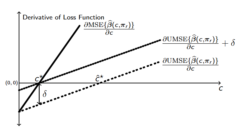
We propose to reduce over-borrowing with a strategy adapted from Firth, (1993) and illustrated in Figure 3. We first describe the main idea. The derivative of the UMSE has a root at $\widehat{c}^{\star}$ that is positively biased for $c^{\star}$. Therefore, for some $\delta>0$, $[\partial\mathsf{UMSE}\{\boldsymbol{\widehat{\beta}}(c,\boldsymbol{\pi}_{r})\}]/(\partial c)+\delta$ has a root at $c^{\star}$. In words, the optimal borrowing $c^{\star}$ is obtained by shifting the UMSE derivative curve up by $\delta$. The shift needed to obtain a root at $c^{\star}$ is

$$\delta=\frac{\partial^{2}}{\partial c^{2}}\mathsf{UMSE}\{\boldsymbol{\widehat{\beta}}(c,\boldsymbol{\pi}_{r})\}(\widehat{c}^{\star}-c^{\star})=2\|\boldsymbol{\Pi}_{r}\{\boldsymbol{K}\boldsymbol{A}(\boldsymbol{\pi}_{r})-\boldsymbol{I}\}\boldsymbol{\tilde{\beta}}\|^{2}(\widehat{c}^{\star}-c^{\star}).$$

As $\widehat{c}^{\star}-c^{\star}$ is unknown, we propose to estimate it with $\widehat{c}^{\star}-\tilde{c}$, where $\tilde{c}$ minimizes BMSE in equation (5). The root of this corrected derivative will reduce borrowing and be closer, on average, to the optimal $c^{\star}$. We show in Section I of the supplement that finding the root of this corrected derivative and selecting a MSE-minimizing $\boldsymbol{\pi}_{r}$ can be achieved by minimizing the loss function

$$\|\boldsymbol{\Pi}\{\boldsymbol{K}\boldsymbol{A}(\boldsymbol{\pi})-\boldsymbol{I}\}\boldsymbol{\tilde{\beta}}\|^{2}-2\frac{\|\boldsymbol{\Pi}\{\boldsymbol{K}\boldsymbol{A}(\boldsymbol{\pi})-\boldsymbol{I}\}\boldsymbol{\tilde{\beta}}\}\|^{2}\times\mathsf{tr}(\mathsf{Cov}[\boldsymbol{\tilde{\beta}},\boldsymbol{\Pi}\{\boldsymbol{K}\boldsymbol{A}(\boldsymbol{\pi})-\boldsymbol{I}\}\boldsymbol{\tilde{\beta}}])}{\mathsf{tr}(\mathsf{Var}[\boldsymbol{\Pi}\{\boldsymbol{K}\boldsymbol{A}(\boldsymbol{\pi})-\boldsymbol{I}\}\boldsymbol{\tilde{\beta}}])+\|\boldsymbol{\Pi}\{\boldsymbol{K}\boldsymbol{A}(\boldsymbol{\pi})-\boldsymbol{I}\}\boldsymbol{\tilde{\beta}}\|^{2}}$$ (17)

as a function of the unconstrained $\boldsymbol{\pi}$.

We refer to equation (17) as the pseudo-MSE, so-named to recognize that it is designed and used only for selecting the shrinkage parameters. The asymptotic results discussed in Section 4 hold under shrinkage parameter selection with the pseudo-MSE, as the minimizer of the pseudo-MSE converges to $c^{\star}$ as $n\to\infty$. We term our final proposed estimator the heterogeneity-adaptive meta-estimator (HAM estimator) $\boldsymbol{\widehat{\beta}}(\boldsymbol{\pi}_{\textsf{HAM}})$ with the shrinkage parameters, $\boldsymbol{\pi}_{\textsf{HAM}}=(\pi_{j,\textsf{HAM}})_{j=1}^{k}$, minimizing equation (17). A simulation study in Section J of the supplement illustrates the performance of $\boldsymbol{\widehat{\beta}}(\boldsymbol{\pi})$ under different shrinkage parameter selection mechanisms.

6 Numerical support

6.1 Overview

In this section, we investigate the performance of the HAM estimator through four simulation settings. In each setting, we compare the HAM estimator $\boldsymbol{\widehat{\beta}}_{\textsf{HAM}}=\boldsymbol{\widehat{\beta}}(\boldsymbol{\pi}_{\textsf{HAM}})$ to the vector of study-specific MLEs $\boldsymbol{\tilde{\beta}}$. We also develop a ridge-like penalized regression competitor $\boldsymbol{\widehat{\beta}}_{\textsf{R}}$ in Section K of the supplement that uses a Euclidean-distance penalty to encourage similar estimates of $\boldsymbol{\beta}$, similar in spirit to the fused ridge estimator (Lettink et al.,, 2023). In each setting, we evaluate $\boldsymbol{\widehat{\beta}}_{\textsf{HAM}},\boldsymbol{\tilde{\beta}}$ and $\boldsymbol{\widehat{\beta}}_{\textsf{R}}$ in $1000$ Monte Carlo replicates. We report the empirical mean squared error (eMSE) and coverage of 95% confidence intervals using equation (14) for the HAM estimator and the large sample distribution of the MLE for $\boldsymbol{\tilde{\beta}}$.

6.2 Setting 1: Varying sample size and number of parameters

We consider a low-heterogeneity setting with $k=3$ studies, $p\in\{2,4,10,20\}$ and ten unique combinations of $n_{j}\in\{100,200,300\}$. Within each Monte Carlo replicate, we generate $n_{j}$ observations $\boldsymbol{X}_{j}$ and error terms $\boldsymbol{\epsilon}_{j}\sim\mathcal{N}(\boldsymbol{0},\boldsymbol{I}_{n_{j}})$: when $p=2$, $\boldsymbol{X}_{1j}=\boldsymbol{1}$, $\boldsymbol{X}_{2j}\sim\mathcal{N}(\boldsymbol{0},\boldsymbol{I}_{n_{j}})$; when $p=4$, we further include $X_{3ij}\sim\text{Bern}(0.5)$, $X_{4ij}=X_{2ij}X_{3ij}$, $i=1,\dots,n_{j}$; when $p=10$ and $p=20$, the additional covariates are simulated independently from standard normal distributions.

The process for generating study-specific parameters intentionally violates a key assumption of random-effects meta-analysis: while the study parameters are generated from the same distribution, they do not come from a normal distribution. Specifically, for each $(n_{1},n_{2},n_{3},p)$ combination, we generate $\boldsymbol{\beta}_{j}=\boldsymbol{\beta}_{m}+\boldsymbol{u}_{j}$ with $\boldsymbol{u}_{j}\in\mathbb{R}^{p}$ independent draws from $\text{Unif}(-0.25,0.25)$ rounded to two decimal places. The values of $\boldsymbol{\beta}_{j}$ are held constant across Monte Carlo replicates in each combination; values of $\boldsymbol{\beta}_{j}$ are included in Table 10 of the supplement. Table 1 displays the eMSE of the three estimators $\boldsymbol{\tilde{\beta}}$, $\boldsymbol{\widehat{\beta}}_{\textsf{HAM}}$, and $\boldsymbol{\widehat{\beta}}_{\textsf{R}}$. Across all combinations, the HAM estimator has a smaller eMSE than the MLE. As sample sizes increase, the ratio of the eMSE for the HAM estimator to the eMSE for the MLE gets closer to 1; at larger sample sizes, the heterogeneity of the datasets is more easily detected and the HAM estimator reverts to the study-specific MLEs, preventing over-borrowing and enabling inference. The HAM estimator also yields a smaller eMSE than the ridge-like estimator across the majority of settings.

	$p=2$			$p=4$			$p=10$			$p=20$
$n_{1},n_{2},n_{3}$	$\boldsymbol{\tilde{\beta}}$	$\boldsymbol{\widehat{\beta}}_{\textsf{HAM}}$	$\boldsymbol{\widehat{\beta}}_{\textsf{R}}$	$\boldsymbol{\tilde{\beta}}$	$\boldsymbol{\widehat{\beta}}_{\textsf{HAM}}$	$\boldsymbol{\widehat{\beta}}_{\textsf{R}}$	$\boldsymbol{\tilde{\beta}}$	$\boldsymbol{\widehat{\beta}}_{\textsf{HAM}}$	$\boldsymbol{\widehat{\beta}}_{\textsf{R}}$	$\boldsymbol{\tilde{\beta}}$	$\boldsymbol{\widehat{\beta}}_{\textsf{HAM}}$	$\boldsymbol{\widehat{\beta}}_{\textsf{R}}$
100, 100, 100	6.3	4.6	4.8	37.4	27.3	28.4	60.8	40.2	41.7	105.5	77.1	76.6
100, 200, 100	5.2	3.8	4.2	31.6	23.8	24.8	50.4	33.7	34.6	85.9	64.4	64.0
100, 200, 200	4.1	3.2	3.6	24.7	18.7	18.9	38.8	27.2	28.4	66.3	51.7	52.2
100, 300, 100	4.8	3.5	3.9	29.4	21.7	22.4	47.4	31.4	32.0	80.9	60.0	59.5
100, 300, 200	3.6	2.8	3.3	23.2	17.3	17.3	35.6	24.6	25.9	60.8	47.1	47.6
100, 300, 300	3.4	2.7	3.2	20.0	14.7	14.5	32.7	22.7	24.4	55.2	43.0	43.5
200, 200, 200	3.0	2.5	2.8	18.5	15.2	15.9	28.8	21.7	22.6	47.0	40.0	40.1
200, 300, 200	2.7	2.3	2.6	16.8	13.8	14.3	25.5	19.4	20.2	41.2	35.4	35.4
200, 300, 300	2.4	2.1	2.3	14.7	12.0	12.2	22.1	17.4	18.5	35.6	31.2	31.6
300, 300, 300	2.0	1.7	1.9	12.2	10.4	10.9	18.6	15.1	15.8	30.0	27.0	27.1

Table 1: Empirical MSEs for each estimator multiplied by 100 for Setting 1. The smallest eMSE for each $(n_{1},n_{2},n_{3},p)$ combination is bolded.

Table 2 reports coverage rates of 95% large-sample confidence intervals using $\boldsymbol{\widehat{\beta}}_{\textsf{HAM}}$. Study-level coverages grow closer to the nominal level with increasing $p$. As the number of covariates increases, our method more easily distinguishes between the study outcome distributions and appropriately decreases the amount of information sharing. Increasing the sample size for one study while holding others constant increases coverage for that study, but can decrease coverage for the others. For example, moving from study sizes $(100,100,100)$ to $(100,200,100)$ increases the coverage for study 2 but decreases the coverage for study 3 because the centroid shifts towards study 2’s outcome distribution, which moves $\boldsymbol{\widehat{\beta}}_{3,\textsf{HAM}}$ further from $\boldsymbol{\beta}_{3}$.

	$p=2$			$p=4$			$p=10$			$p=20$
$n$	$\boldsymbol{\beta}_{1}$	$\boldsymbol{\beta}_{2}$	$\boldsymbol{\beta}_{3}$	$\boldsymbol{\beta}_{1}$	$\boldsymbol{\beta}_{2}$	$\boldsymbol{\beta}_{3}$	$\boldsymbol{\beta}_{1}$	$\boldsymbol{\beta}_{2}$	$\boldsymbol{\beta}_{3}$	$\boldsymbol{\beta}_{1}$	$\boldsymbol{\beta}_{2}$	$\boldsymbol{\beta}_{3}$
100, 100, 100	87.9	92.6	89.7	93.3	90.4	89.8	93.0	91.7	92.4	92.3	92.2	92.0
100, 200, 100	88.6	93.1	88.5	92.4	91.5	88.5	92.6	91.9	91.0	91.9	93.2	91.5
100, 200, 200	85.2	93.3	90.6	92.2	90.3	89.0	92.5	91.0	91.6	92.0	92.8	92.5
100, 300, 100	86.5	93.8	88.8	92.8	92.9	86.8	91.7	92.9	90.2	91.8	93.7	91.5
100, 300, 200	85.4	94.3	90.5	91.8	90.2	87.9	92.6	91.7	91.2	91.4	93.6	92.2
100, 300, 300	84.5	93.2	90.6	92.9	90.1	89.3	91.9	90.6	91.7	91.2	93.4	92.8
200, 200, 200	89.2	92.0	89.3	92.4	90.1	90.0	93.0	91.6	92.2	92.7	92.5	92.9
200, 300, 200	86.6	93.2	87.5	91.5	90.5	89.8	92.7	92.5	91.4	92.5	93.4	92.5
200, 300, 300	85.9	92.8	90.0	92.0	90.9	89.8	92.5	91.5	92.0	92.4	93.4	92.9
300, 300, 300	89.0	92.3	89.4	92.2	91.1	90.5	93.1	91.6	92.0	93.2	93.3	93.1

Table 2: Average coverage rate (%) of 95% confidence intervals using $\boldsymbol{\widehat{\beta}}_{\textsf{HAM}}$ in Setting 1.

6.3 Setting 2: Varying number of studies and heterogeneity

We now examine the HAM estimator’s performance with $p=4$ parameters as the number of studies $k\in\{5,10,15\}$ increases under varying parameter heterogeneity conditions. In the first condition, there is no heterogeneity and $\boldsymbol{\beta}_{j}\equiv\boldsymbol{\beta}_{m}$, $j=1,\ldots,k$. In the second, the $\boldsymbol{\beta}_{j}$ display mild heterogeneity with $\boldsymbol{\beta}_{j}\sim\mathcal{N}(\boldsymbol{\beta}_{m},.1\boldsymbol{I}_{4})$. The $\boldsymbol{\beta}_{j}$ in the third condition are moderately heterogeneous: $\boldsymbol{\beta}_{j}\sim\mathcal{N}(\boldsymbol{\beta}_{m},.5\boldsymbol{I}_{4})$. Finally, the $\boldsymbol{\beta}_{j}$ in the fourth condition have a mixture of no heterogeneity and high heterogeneity: $\boldsymbol{\beta}_{j}\equiv\boldsymbol{\beta}_{m}$ for $j=1,2,3$ and $\boldsymbol{\beta}_{j}\sim\mathcal{N}(\boldsymbol{\beta}_{m},\boldsymbol{I}_{4})$ for $j=4,\ldots,k$. We emulate the study parameter generation process assumed for random-effects meta-analysis by drawing new values of $\boldsymbol{\beta}_{j}$ with each Monte Carlo replicate. For each Monte Carlo replicate, we generate $n_{j}=200$ observations $\boldsymbol{X}_{j}$ and error terms, $\boldsymbol{\epsilon}_{j}\sim\mathcal{N}(\boldsymbol{0},\boldsymbol{I}_{n_{j}})$ following $\boldsymbol{X}_{1j}=\boldsymbol{1}$, $\boldsymbol{X}_{2j}\sim\mathcal{N}(\boldsymbol{0},\boldsymbol{I}_{n_{j}})$, $X_{3ij}\sim\text{Bern}(.5)$ and $X_{4ij}=X_{2ij}X_{3ij}$, $i=1,\dots,n_{j}$.

Table 3 displays the eMSE of $\boldsymbol{\tilde{\beta}}$, $\boldsymbol{\widehat{\beta}}_{\textsf{HAM}}$, and $\boldsymbol{\widehat{\beta}}_{\textsf{R}}$ and the coverage rate of $\boldsymbol{\widehat{\beta}}_{\textsf{HAM}}$’s large-sample 95% confidence interval. The coverage is closest to its nominal value in the condition with complete homogeneity and is furthest in the condition with mild heterogeneity. In the mild heterogeneity condition, the study outcome distributions are close together, and our method consequently over-borrows. Across all combinations of heterogeneity and $k$, $\boldsymbol{\widehat{\beta}}_{\textsf{HAM}}$ has eMSE less than or equal to that of $\boldsymbol{\tilde{\beta}}$. The HAM estimator’s eMSE is slightly larger than $\boldsymbol{\widehat{\beta}}_{\textsf{R}}$’s with no, mild or moderate heterogeneity, but is smaller than $\boldsymbol{\widehat{\beta}}_{\textsf{R}}$’s in the mixture condition due to the added flexibility of study-specific shrinkage parameters. A smaller eMSE is only desirable, however, if the inference is calibrated, and the ridge-like estimator has no inferential guarantees.

		eMSE$\times 100$			Coverage rate (%)
Heterogeneity	$k$	$\boldsymbol{\tilde{\beta}}$	$\boldsymbol{\widehat{\beta}}_{\textsf{HAM}}$	$\boldsymbol{\widehat{\beta}}_{\textsf{R}}$	$\boldsymbol{\widehat{\beta}}_{\textsf{HAM}}$
None	5	29.9	12.6	8.1	94.5
	10	62.1	21.3	8.4	94.4
	15	92.5	28.6	7.5	94.8
Mild	5	30.5	28.3	27.1	91.1
	10	61.3	56.1	52.2	90.9
	15	91.9	83.7	77.7	90.9
Moderate	5	30.8	30.8	30.0	93.2
	10	61.4	61.3	59.1	93.0
	15	92.8	92.5	89.4	92.7
Mixture	5	30.6	24.4	29.2	92.7
	10	61.4	55.8	59.9	92.9
	15	92.0	86.0	89.6	93.3

Table 3: Empirical MSEs for each estimator (multiplied by 100) and coverage rate of 95% confidence intervals using $\boldsymbol{\widehat{\beta}}_{\textsf{HAM}}$ in setting 2.

Examining the selected shrinkage parameters $\boldsymbol{\pi}_{\textsf{HAM}}$ provides additional insight into the information-borrowing mechanism. Figure 4 shows the distribution of $\boldsymbol{\pi}_{\textsf{HAM}}$ for each heterogeneity condition across replicates when $k=15$. In the condition with no heterogeneity, the selected $\boldsymbol{\pi}_{\textsf{HAM}}$ are centered around $0.5$, which is slightly more conservative than the MSE-minimizing $\pi_{j}$ of $1$. In the mixture condition, the $\pi_{\textsf{HAM},j}$ associated with the homogeneous studies are separated from the $\pi_{\textsf{HAM},j}$ associated with the heterogeneous studies, as desired.

Figure 4: $\boldsymbol{\pi}_{\textsf{HAM}}$ values across heterogeneity conditions when $k=15$ in setting 2.

6.4 Setting 3: Meta-analysis with overlapping covariates

Meta-analyses often combine the effect sizes for a shared covariate of interest after controlling for any relevant covariates at the study-level, as described in Section 3.2. We consider $k=20$ studies ($n_{j}=200,j=1,\ldots,20$) with $p=1$ and $q_{j}=4$ where all studies share the first covariate but the other covariates vary across studies. We consider two scenarios for the generation of $\beta_{j}$, the coefficient of interest. In the first scenario, $\beta_{j}$ is drawn from a single distribution, $\beta_{j}=3.47+u_{j}$ with $u_{j}\sim\text{Unif}(-0.25,0.25)$. In the second, more challenging scenario, $\beta_{j}$ is drawn from one of two distributions, $\beta_{j}\sim\text{Unif}(-0.25,0.25)$ for $j=1,\dots,5$ and $\beta_{j}=3.47+u_{j}$, $u_{j}\sim\text{Unif}(-0.25,0.25)$ for $j=6,\dots,20$. Values of $\boldsymbol{\gamma}_{j}$ are independently drawn from $\mathcal{N}(\boldsymbol{0},\boldsymbol{I}_{4})$. All parameter values are rounded to two decimal places and held constant over Monte Carlo replicates. The first, shared covariate is an intercept and the remaining covariates are simulated independently from standard normal distributions. Error terms are generated independently from standard normal distributions.

Table 4 displays the eMSE for $\boldsymbol{\tilde{\beta}}$, $\boldsymbol{\widehat{\beta}}_{\textsf{HAM}}$, and $\boldsymbol{\widehat{\beta}}_{\textsf{R}}$. In both scenarios, the eMSE of $\boldsymbol{\widehat{\beta}}_{\textsf{HAM}}$ is smaller than the eMSE of $\boldsymbol{\tilde{\beta}}$. When $\beta_{j}$ are drawn from a single distribution, $\boldsymbol{\widehat{\beta}}_{\textsf{HAM}}$ and $\boldsymbol{\widehat{\beta}}_{\textsf{R}}$ have similar eMSEs. As in Setting 2 (Section 6.3), $\boldsymbol{\widehat{\beta}}_{\textsf{HAM}}$ outperforms $\boldsymbol{\widehat{\beta}}_{\textsf{R}}$ when $\beta_{j}$ is drawn from one of two distributions.

$\beta_{j}$ scenario	eMSE$\times 100$			Coverage rate using $\boldsymbol{\widehat{\beta}}_{\textsf{HAM}}$ (%)
	$\boldsymbol{\tilde{\beta}}$	$\boldsymbol{\widehat{\beta}}_{\textsf{HAM}}$	$\boldsymbol{\widehat{\beta}}_{\textsf{R}}$
Single distribution	10.4	8.2	8.1	83.8
Two distributions	10.4	9.1	10.3	87.3

Table 4: Empirical MSEs for each estimator (multiplied by 100) and coverage of 95% confidence intervals using $\boldsymbol{\widehat{\beta}}_{\textsf{HAM}}$ in setting 3.

Table 4 also reports the coverage rate of $\boldsymbol{\widehat{\beta}}_{\textsf{HAM}}$’s large-sample 95% confidence interval. We investigate the observed undercoverage in Figure 5, where we plot the coverage of $\widehat{\beta}_{\textsf{HAM},j}$ versus $\beta_{j}$; we use colour to denote which quartile the average (across the 1000 Monte Carlo replicates) $\pi_{j,\textsf{HAM}}$ belongs to, with the quartiles computed across all studies. When $\beta_{j}$ is drawn from a single distribution, studies with $\beta_{j}$ values closest to $3.47$, the center of the distribution, have the largest average $\pi_{j,\textsf{HAM}}$ and coverage nearest to the nominal level. When $\beta_{j}$ is drawn from one of two distributions, the coverage is closer to the nominal level for the five studies with $\beta_{j}\sim\text{Unif}(-0.25,0.25)$. These studies are far enough away from the others that their selected shrinkage parameters are close to zero. In both scenarios, coverage is lower for studies where the parameter is not too far from $3.47$. As a rule of thumb, our estimator tends to over-borrow in situations where it struggles to distinguish between studies because the MLEs are close to each other. Increasing the dimension $p$ or the sample size alleviates this issue, as seen in setting 1 (Section 6.2).

Figure 5: Coverage of $\widehat{\beta}_{\textsf{HAM},j}$ versus $\beta_{j}$ for each study in setting 3.

6.5 Setting 4: Varying covariate data generation process

We investigate the performance of $\boldsymbol{\widehat{\beta}}_{\textsf{HAM}}$ in the presence of population heterogeneity by varying the covariate data generation process. We consider $k=3$ studies with $p=4$ covariates each, and generate $\boldsymbol{\beta}_{j}\sim\text{Unif}(-0.25,0.25)$, rounding to two decimal places and holding these values constant over the Monte Carlo replicates. The sample sizes are $n_{j}\equiv n\in\{20,50,100,200,500\}$ and the error terms are $\boldsymbol{\epsilon}_{j}\sim\mathcal{N}(\boldsymbol{0},\sigma^{2}_{j}\boldsymbol{I}_{n})$. In each study, $\boldsymbol{X}_{j}$ has a column of ones for the intercept with the remaining covariates independently generated from $\mathcal{N}(\mu_{j},b^{2}\boldsymbol{I}_{p-1})$, with $b=1$ when $\mu_{j}=0$ and $b=\mu_{j}$ otherwise. We consider four scenarios for $\boldsymbol{\mu}=(\mu_{1},\mu_{2},\mu_{3})$ and $\boldsymbol{\sigma}^{2}=(\sigma_{1}^{2},\sigma_{2}^{2},\sigma_{3}^{3})$: (i) $\boldsymbol{\mu}=(0,0,0)$, $\boldsymbol{\sigma}^{2}=(1,1,1)$; (ii) $\boldsymbol{\mu}=(10,10,10)$, $\boldsymbol{\sigma}^{2}=(100,100,100)$; (iii) $\boldsymbol{\mu}=(0,1,2)$, $\boldsymbol{\sigma}^{2}=(1,1,4)$; (iv) $\boldsymbol{\mu}=(0,5,10)$, $\boldsymbol{\sigma}^{2}=(1,25,100)$. Across every setting, the variation of the error term is equal to the variation in the non-intercept covariates to allow us to isolate the impact of increasing the scale of the non-intercept covariates.

Table 5 displays the eMSE and coverage rate of 95% asymptotic confidence intervals. Scenarios (ii) and (iv), each having at least one study with $\mu_{j}=10$, have lower coverage than the nominal rate even as the sample size grows large. These scenarios also show a greater reduction in eMSE relative to the MLE at large sample sizes, compared to scenarios (i) and (iii). To diagnose the coverage issue we examine the 95% confidence intervals of $\boldsymbol{\tilde{\beta}}$ at $n=500$ in Figure 6. The overlap in confidence intervals for the intercept coefficient $\beta_{1}$ in scenarios (ii) and (iv) is leading our estimator to over-borrow, yielding large reductions in eMSE at the expense of coverage.

	scenario (i)				scenario (ii)				scenario (iii)				scenario (iv)
	eMSE$\times 100$			CR	eMSE$\times 100$			CR	eMSE$\times 100$			CR	eMSE$\times 100$			CR
n	$\boldsymbol{\tilde{\beta}}$	$\boldsymbol{\widehat{\beta}}_{\textsf{HAM}}$	$\boldsymbol{\widehat{\beta}}_{\textsf{R}}$	$\boldsymbol{\widehat{\beta}}_{\textsf{HAM}}$	$\boldsymbol{\tilde{\beta}}$	$\boldsymbol{\widehat{\beta}}_{\textsf{HAM}}$	$\boldsymbol{\widehat{\beta}}_{\textsf{R}}$	$\boldsymbol{\widehat{\beta}}_{\textsf{HAM}}$	$\boldsymbol{\tilde{\beta}}$	$\boldsymbol{\widehat{\beta}}_{\textsf{HAM}}$	$\boldsymbol{\widehat{\beta}}_{\textsf{R}}$	$\boldsymbol{\widehat{\beta}}_{\textsf{HAM}}$	$\boldsymbol{\tilde{\beta}}$	$\boldsymbol{\widehat{\beta}}_{\textsf{HAM}}$	$\boldsymbol{\widehat{\beta}}_{\textsf{R}}$	$\boldsymbol{\widehat{\beta}}_{\textsf{HAM}}$
20	77.5	44.8	40.2	91.1	7756.1	4320.0	3569.1	91.4	198.7	100.0	92.0	90.4	3262.6	1427.1	997.3	90.3
50	25.9	17.7	17.7	91.7	2771.6	1631.6	1383.8	90.1	66.3	37.9	34.7	90.0	1120.9	477.6	355.8	87.6
100	12.6	10.0	10.4	91.1	1240.9	719.4	593.9	87.3	31.5	20.9	17.9	88.4	539.3	233.3	172.3	83.2
200	6.2	5.5	5.6	91.2	624.5	375.5	309.2	81.5	15.9	12.4	9.8	87.9	255.5	114.0	83.5	76.9
500	2.4	2.3	2.3	92.5	246.3	151.5	120.7	69.6	6.0	5.8	4.3	88.8	104.2	52.5	36.7	69.1

Table 5: Empirical MSEs, multiplied by 100, and coverage rate (CR, %) for 95% confidence intervals in simulation setting 4.

Figure 6: Average 95% confidence intervals at $n=500$ for $\boldsymbol{\tilde{\beta}}$. In scenarios (ii) and (iv), the confidence intervals for the intercept, $\beta_{1}$, overlap substantially.

We remedy the over-borrowing by computing $\boldsymbol{\widehat{\beta}}_{\textsf{HAM}}$ using data that have been rescaled so that each non-intercept covariate has a standard deviation of $1$. This standardization prevents the intercept covariate from becoming overly informative, and can be done without accessing the raw data when the standard deviation for each covariate is available, which is usually the case in practice. The results are shown in Table 6. Across all scenarios, the eMSE improvement on the standardized data is smaller than on the original data and the coverage approaches the nominal level faster as $n$ grows. We thus recommend this simple rescaling as a general pre-processing step to improve the finite-sample performance of our estimator.

	scenario (i)			scenario (ii)			scenario (iii)			scenario (iv)
	eMSE$\times 100$		CR	eMSE$\times 100$		CR	eMSE$\times 100$		CR	eMSE$\times 100$		CR
n	$\boldsymbol{\tilde{\beta}}$	$\boldsymbol{\widehat{\beta}}_{\textsf{HAM}}$	$\boldsymbol{\widehat{\beta}}_{\textsf{HAM}}$	$\boldsymbol{\tilde{\beta}}$	$\boldsymbol{\widehat{\beta}}_{\textsf{HAM}}$	$\boldsymbol{\widehat{\beta}}_{\textsf{HAM}}$	$\boldsymbol{\tilde{\beta}}$	$\boldsymbol{\widehat{\beta}}_{\textsf{HAM}}$	$\boldsymbol{\widehat{\beta}}_{\textsf{HAM}}$	$\boldsymbol{\tilde{\beta}}$	$\boldsymbol{\widehat{\beta}}_{\textsf{HAM}}$	$\boldsymbol{\widehat{\beta}}_{\textsf{HAM}}$
20	71.4	58.7	89.3	13073.0	9842.3	88.5	246.0	227.3	88.9	5447.7	5269.2	90.2
50	25.1	21.2	91.0	4697.8	3739.3	89.1	84.4	80.4	92.2	1919.6	1889.2	92.8
100	12.4	10.9	91.5	2150.5	1768.2	89.8	40.3	38.8	92.6	919.4	919.8	94.3
200	6.1	5.7	91.5	1074.3	914.9	90.1	20.5	19.8	92.8	440.0	441.9	94.5
500	2.4	2.3	92.8	426.2	390.8	91.0	7.8	7.7	92.8	178.2	178.7	94.9

Table 6: Empirical MSEs, multiplied by 100, and coverage rate (CR, %) of 95% confidence intervals in simulation setting 4 on rescaled data.

7 Real data analysis

We illustrate the practical advantages of the HAM estimator in a meta-analysis of covariates of intensive-care unit (ICU) length of stay using real data from the eICU Collaborative Research Database (Pollard et al.,, 2019). Section M in the supplement describes the access procedure for these data. Longer ICU stays are associated with higher healthcare costs and adverse health outcomes, including an increased risk of mortality after discharge (Williams et al.,, 2010; Moitra et al.,, 2016). Anticipating and reducing the length of stay is also valuable to hospitals for resource management, especially in the presence of ICU bed shortages (Rapoport et al.,, 2003; Bai et al.,, 2018). We investigate the association between ICU length of stay and a set of covariates measured at admission to the ICU across multiple hospitals. Fitting a random-effects meta-analysis requires unverifiable assumptions on the distribution of hospital-level parameters, but fitting hospital-level models individually does not take full advantage of similarities between hospitals. The HAM estimator provides inference for each hospital while also allowing information borrowing to improve precision.

We conduct the meta-analysis using the log transform of the ICU length of stay as the outcome. We assess the association between length of stay and a patient’s age, gender, systolic and diastolic blood pressure when entering the ICU, whether a patient was admitted from the emergency department (ED) or from another source, and the Acute Physiology and Chronic Health Evaluation (APACHE) IV score. The APACHE IV score incorporates clinical and health history data collected from patients within the first day in the ICU, but it is designed with ICU mortality as the primary outcome (Zimmerman et al.,, 2006). Prior work indicates that the APACHE IV score is a poor predictor of ICU length of stay; we include it in our model to help account for initial health status and to assess whether the association between the score and length of stay varies across hospitals (Verburg et al.,, 2014; Zangmo and Khwannimit,, 2023). We consider only patients discharged alive from the ICU. Our data consist of $k=29$ hospitals from the West region of the eICU database for which there were at least 100 patients recorded as discharged alive from the ICU in 2014 and 2015. We standardize the continuous predictors as discussed in Section 6.5.

A preliminary examination shows substantial heterogeneity among hospitals ($I^{2}=79.6\%$) suggesting that conducting a traditional meta-analysis is not meaningfully interpretable. To implement our method, we find the vector $\boldsymbol{\pi}_{\textsf{HAM}}$ that minimizes the pseudo-MSE in equation (17). As visualized in Figure 7, the majority of hospitals have $\pi_{j,\textsf{HAM}}$ between 0.3 and 0.5, while four hospitals have a smaller $\pi_{j,\textsf{HAM}}$. The variability in $\boldsymbol{\pi}_{\textsf{HAM}}$ echoes the large $I^{2}$; we would expect to see $\pi_{j,\textsf{HAM}}$ close to 0.5 for all studies in the presence of homogeneity. Using $\boldsymbol{\pi}_{\textsf{HAM}}$, we first compare the estimated centroid $\boldsymbol{\widehat{\theta}}(\boldsymbol{\pi}_{\textsf{HAM}})$ to results from fixed- and random-effect meta-analyses in Table 7, which displays the 95% confidence intervals for the meta-estimates (the confidence interval using $\boldsymbol{\widehat{\theta}}(\boldsymbol{\pi}_{\textsf{HAM}})$ is constructed using the distribution of the MLE $\boldsymbol{\tilde{\beta}}$). While the fixed- and random-effect confidence intervals give inference on a shared parameter $\boldsymbol{\beta}_{m}$, the confidence interval for $\boldsymbol{\widehat{\theta}}(\boldsymbol{\pi}_{\textsf{HAM}})$ is built to capture the true value of the centroid $\boldsymbol{\theta}$, which is not necessarily equal to $\boldsymbol{\beta}_{m}$. Nevertheless, in this case, the three confidence intervals cover similar regions.

To show the efficiency gain from borrowing information across studies, we compare the study-specific MLEs to the HAM estimates, $\boldsymbol{\widehat{\beta}}(\boldsymbol{\pi}_{\textsf{HAM}})$. Table 8 reports the result of hypothesis tests by covariate and, as expected, in all but one case the HAM estimates are more often significant at level $\alpha=0.05$. In particular, the “age” and “admission from an ED” effect estimates gain statistical significance using HAM for several hospitals. Figure 7 plots the HAM and MLE confidence intervals for $\beta_{\text{APACHE IV}}$ with the corresponding $\pi_{j,\textsf{HAM}}$. Estimates for hospitals with high $\pi_{j,\textsf{HAM}}$ experience a large shift in their point estimate toward the centroid estimate, as well as a reduction in the width of the corresponding confidence interval. Figure 8 displays the 95% confidence intervals for all covariates, with hospitals sorted from smallest to largest $\pi_{j,\textsf{HAM}}$. Changes in significance between the MLE and HAM estimators are more frequent as $\pi_{j,\textsf{HAM}}$ increases, reflecting the decrease in variance with more information sharing.

Overall, an increasing APACHE IV score, indicative of worse clinical condition at ICU entry, is associated with a longer ICU length of stay for all hospitals. In fact, out of the selected covariates, the APACHE IV score is the only one which is significantly related to the log-transformed length of stay for all hospitals using the HAM estimator. All else held constant, patients admitted from the ED tend to have shorter stays in the ICU than other patients, for most hospitals. Counterintuitively, for most hospitals, older patients also have shorter stays in the ICU after accounting for other covariates. This result is perhaps a by-product of keeping only patients who are discharged alive; filtering disproportionately removes older individuals with longer ICU stays.

	Fixed-Effect		Random-Effect		$\boldsymbol{\widehat{\theta}}(\boldsymbol{\pi}_{\textsf{HAM}})$
Covariate	Lower	Upper	Lower	Upper	Lower	Upper
Intercept	0.475	0.527	0.479	0.632	0.498	0.553
Gender	$-$0.016	0.040	$-$0.012	0.069	$-$0.003	0.056
Admission from ED	$-$0.083	$-$0.027	$-$0.146	$-$0.040	$-$0.126	$-$0.067
APACHE IV score	0.344	0.374	0.329	0.381	0.348	0.379
Age	$-$0.091	$-$0.060	$-$0.094	$-$0.055	$-$0.089	$-$0.057
Diastolic BP	0.020	0.057	0.023	0.064	0.024	0.064
Systolic BP	$-$0.055	$-$0.017	$-$0.063	$-$0.019	$-$0.057	$-$0.018

Table 7: Lower and upper bounds of 95% confidence intervals for meta-estimators.

Figure 7: Hospital-level 95% confidence intervals for $\beta_{\textrm{APACHE IV}}$ using $\boldsymbol{\widehat{\beta}}(\boldsymbol{\pi}_{\textsf{HAM}})$ and $\boldsymbol{\tilde{\beta}}$, and corresponding $\pi_{j,\textsf{HAM}}$. Hospitals are ordered from smallest to largest MLE.

Figure 8: 95% confidence intervals for each coefficient using the HAM estimator with significance at level $0.05$ using both HAM and MLE estimators. Hospitals are ordered from smallest to largest $\pi_{j,\textsf{HAM}}$.

	$p_{\textsf{HAM}}\leq 0.05$		$p_{\textsf{HAM}}>0.05$
Covariate	$p_{\textsf{MLE}}\leq 0.05$	$p_{\textsf{MLE}}>0.05$	$p_{\textsf{MLE}}\leq 0.05$	$p_{\textsf{MLE}}>0.05$
Intercept	1	0	2	26
Gender	26	0	0	3
Admission from ED	16	1	7	5
APACHE IV Score	0	0	1	28
Age	9	0	9	11
Diastolic BP	23	0	1	5
Systolic BP	26	0	0	3

Table 8: Hypothesis test results across $k=29$ hospitals for each coefficient versus a null hypothesis of $0$. The $p_{\textsf{HAM}}$ and $p_{\textsf{MLE}}$ denote $p$-values for each covariate effect using the HAM and MLE, respectively.

8 Conclusion

Several unique aspects of our proposal bear emphasizing. First, we introduce a new centroid as the data-sharing mechanism that links estimates from individual studies. This centroid symmetrizes the transfer learning inferential goal to adapt it to the meta-analysis setting, and its estimation introduces important flexibility for data-adaptive borrowing. Study-specific shrinkage parameters further allow our estimator to differentially borrow according to a study’s similarity to the centroid. Second, our use of a Kullback-Leibler divergence shrinkage penalty leads to intuitive and interpretable estimators with the familiar fixed-effect meta-estimator as a special case. Third, by carefully choosing the amount of shrinkage, our estimator is both more efficient than the MLE in finite samples and has large-sample inferential guarantees critical for practical use. The proof of these properties relies on an important new parameterization that decouples the selection of the centroid from the selection of the amount of shrinkage. Finally, while data integration methods often rely on cross-validation or raw data access to estimate the optimal amount of data sharing (e.g. Han et al.,, 2025; Wu and Yang,, 2023), our new approach relies on a bias-reduced estimator of shrinkage parameters that balances both finite-sample and asymptotic bias. Put together, these results bestow on our estimator data-adaptive flexibility with statistical efficiency guarantees that preserve practical advantages.

One limitation of the HAM estimator is that it requires the complete covariance matrix for the study-specific MLEs. While it may not be always readily available, it contains no participant-level data and can therefore be shared without violating data privacy. In fact, practitioners have advocated for its automatic inclusion in publications (Zientek and Thompson,, 2009). Empirically, we also found evidence that our estimator’s large-sample properties benefit from standardized covariate inputs. These can be obtained without access to the raw data when the standard deviations of covariates are reported, as is usually the case.

Future work should focus on extending the HAM estimator to generalized linear models to enable its implementation in a wider variety of models. Future work may also consider different inferential goals and investigate the theoretical and empirical properties of the HAM estimator when selecting shrinkage parameters using a different loss function than the MSE. For example, one could instead select $\boldsymbol{\pi}$ to minimize the mean squared prediction error or the MSE for a subset of study effects. We leave these open questions to the interested reader.

Appendix A Derivation of estimators

In this section, we derive the estimators in equations (3) and (4) of the main manuscript, as well as those in Section 3.2. We derive these estimators for the general case where study $j$ has $q_{j}$ covariates, $p$ of which are common across studies.

In this context, for study $j$, denote the $n_{j}\times p$ matrix for the effects of interest as $\boldsymbol{X}_{j}$ and denote the $n_{j}\times(q_{j}-p)$ matrix of control covariates as $\boldsymbol{Z}_{j}$. Outcomes for study $j$ are modeled as

$$\boldsymbol{Y}_{j}=\boldsymbol{X}_{j}\boldsymbol{\beta}_{j}+\boldsymbol{Z}_{j}\boldsymbol{\gamma}_{j}+\epsilon_{j},\quad\epsilon_{j}\sim N(\boldsymbol{0},\sigma_{j}^{2}\boldsymbol{I}_{n_{j}}).$$ (18)

Let $\boldsymbol{K}=\boldsymbol{1}_{k}\otimes\boldsymbol{I}_{p}\in\mathbb{R}^{pk\times p}$ matrix which stacks the vector to its right, and define $\boldsymbol{\Pi}\text{block-diag}\{\pi_{1}\boldsymbol{I}_{p},\ldots,\pi_{k}\boldsymbol{I}_{p}\}\in\mathbb{R}^{pk\times pk}$. As in Section 3.2, define $\boldsymbol{M}_{j}=\boldsymbol{I}_{n_{j}}-\boldsymbol{Z}_{j}(\boldsymbol{Z}_{j}^{\top}\boldsymbol{Z}_{j})^{-1}\boldsymbol{Z}_{j}^{\top}$ when $q_{j}>p$, and $\boldsymbol{M}_{j}=\boldsymbol{I}_{n_{j}}$ when $q_{j}=p$. Let $\boldsymbol{Y}=(\boldsymbol{Y}_{1},\ldots,\boldsymbol{Y}_{k})$, $\boldsymbol{X}=\text{block-diag}\{\boldsymbol{X}_{1},\ldots,\boldsymbol{X}_{k}\}$, $\boldsymbol{M}=\text{block-diag}\{\boldsymbol{M}_{1},\ldots,\boldsymbol{M}_{k}\}$, and $\boldsymbol{\Sigma}=\text{block-diag}\{\sigma_{1}^{2}\boldsymbol{I}_{n_{1}},\ldots,\sigma^{2}_{k}\boldsymbol{I}_{n_{k}}\}$.

First, note that we can change the multiplication order for some sets of matrices:

$$\boldsymbol{\Pi}\boldsymbol{X}^{\top}\boldsymbol{M}\boldsymbol{\Sigma}^{-1}\boldsymbol{M}\boldsymbol{X} =\boldsymbol{X}^{\top}\boldsymbol{M}\boldsymbol{\Sigma}^{-1}\boldsymbol{M}\boldsymbol{X}\boldsymbol{\Pi}$$

$$(\boldsymbol{I}_{pk}-\boldsymbol{\Pi})\boldsymbol{X}^{\top}\boldsymbol{M}\boldsymbol{\Sigma}^{-1}\boldsymbol{M}\boldsymbol{X} =\boldsymbol{X}^{\top}\boldsymbol{M}\boldsymbol{\Sigma}^{-1}\boldsymbol{M}\boldsymbol{X}(\boldsymbol{I}_{pk}-\boldsymbol{\Pi}).$$

Next, as the objective function in equation (3.2) contains the generalized inverse for $\boldsymbol{M}_{j}$, we can write

$$(\boldsymbol{M}_{j}\boldsymbol{Y}_{j}-\boldsymbol{M}_{j}\boldsymbol{X}_{j}\boldsymbol{\beta}_{j})^{\top}\boldsymbol{M}_{j}^{+} (\boldsymbol{M}_{j}\boldsymbol{Y}_{j}-\boldsymbol{M}_{j}\boldsymbol{X}_{j}\boldsymbol{\beta}_{j})$$

$$=(\boldsymbol{Y}_{j}-\boldsymbol{X}_{j}\boldsymbol{\beta}_{j})^{\top}\boldsymbol{M}_{j}\boldsymbol{M}_{j}^{\top}\boldsymbol{M}_{j}(\boldsymbol{Y}_{j}-\boldsymbol{X}_{j}\boldsymbol{\beta}_{j})$$

$$=(\boldsymbol{Y}_{j}-\boldsymbol{X}_{j}\boldsymbol{\beta}_{j})^{\top}\boldsymbol{M}_{j}(\boldsymbol{Y}_{j}-\boldsymbol{X}_{j}\boldsymbol{\beta}_{j})$$

$$=(\boldsymbol{M}_{j}\boldsymbol{Y}_{j}-\boldsymbol{M}_{j}\boldsymbol{X}_{j}\boldsymbol{\beta}_{j})^{\top}(\boldsymbol{M}_{j}\boldsymbol{Y}_{j}-\boldsymbol{M}_{j}\boldsymbol{X}_{j}\boldsymbol{\beta}_{j}).$$

Using this, we maximize the objective function

$$O(\boldsymbol{\beta},\boldsymbol{\theta};\boldsymbol{\Pi})= -\frac{1}{2}(\boldsymbol{M}\boldsymbol{Y}-\boldsymbol{M}\boldsymbol{X}\boldsymbol{\beta})^{\prime}\boldsymbol{\Sigma}^{-1}(\boldsymbol{M}\boldsymbol{Y}-\boldsymbol{M}\boldsymbol{X}\boldsymbol{\beta})$$

$$\quad-\frac{1}{2}(\boldsymbol{\beta}-\boldsymbol{K}\boldsymbol{\theta})^{\prime}\boldsymbol{\Pi}(\boldsymbol{I}-\boldsymbol{\Pi})^{-1}\boldsymbol{X}^{\top}\boldsymbol{M}\boldsymbol{\Sigma}^{-1}\boldsymbol{M}\boldsymbol{X}(\boldsymbol{\beta}-\boldsymbol{K}\boldsymbol{\theta}),$$

with respect to $\boldsymbol{\theta}$ and $\boldsymbol{\beta}$. This is the objective function in equation (2) from Section 3 in matrix form. We begin by taking the partial derivative of the objective function with respect to $\boldsymbol{\theta}$:

$$\nabla_{\boldsymbol{\theta}}O(\boldsymbol{\beta},\boldsymbol{\theta};\boldsymbol{\lambda}) =-\frac{1}{2}\{-2\boldsymbol{K}^{\prime}\boldsymbol{\Pi}(\boldsymbol{I}_{pk}-\boldsymbol{\Pi})^{-1}\boldsymbol{X}^{\top}\boldsymbol{M}\boldsymbol{\Sigma}^{-1}\boldsymbol{M}\boldsymbol{X}(\boldsymbol{\beta}-\boldsymbol{K}\boldsymbol{\theta})\}.$$

The root of this gradient is given by

$$\boldsymbol{\widehat{\theta}}(\boldsymbol{\pi}) =\{\boldsymbol{K}^{\prime}\boldsymbol{\Pi}(\boldsymbol{I}_{pk}-\boldsymbol{\Pi})^{-1}\boldsymbol{X}^{\top}\boldsymbol{M}\boldsymbol{\Sigma}^{-1}\boldsymbol{M}\boldsymbol{X}\boldsymbol{K}\}^{-1}\boldsymbol{K}^{\prime}\boldsymbol{\Pi}(\boldsymbol{I}_{pk}-\boldsymbol{\Pi})^{-1}\boldsymbol{X}^{\top}\boldsymbol{M}\boldsymbol{\Sigma}^{-1}\boldsymbol{M}\boldsymbol{X}\boldsymbol{\widehat{\beta}}(\boldsymbol{\pi})$$

$$=\biggl\{\sum_{j=1}^{d}\frac{\pi_{j}}{(1-\pi_{j})\sigma_{j}^{2}}\boldsymbol{X}_{j}^{\prime}\boldsymbol{M}_{j}\boldsymbol{X}_{j}\biggl\}^{-1}\sum_{j=1}^{d}\frac{\pi_{j}}{(1-\pi_{j})\sigma_{j}^{2}}\boldsymbol{X}_{j}^{\prime}\boldsymbol{M}_{j}\boldsymbol{X}_{j}\boldsymbol{\widehat{\beta}}_{j}(\boldsymbol{\pi}).$$ (19)

We will show that this can be simplified after obtaining a closed form for $\boldsymbol{\widehat{\beta}}(\boldsymbol{\pi})$, discussed next.

The next step is to derive the $\boldsymbol{\widehat{\beta}}(\boldsymbol{\pi})$ that maximizes $O(\boldsymbol{\beta},\boldsymbol{\theta};\boldsymbol{\lambda})$. In the derivation below, we suppress the dependence of $\boldsymbol{\widehat{\beta}}(\boldsymbol{\pi})$ and $\boldsymbol{\widehat{\theta}}(\boldsymbol{\pi})$ on $\boldsymbol{\pi}$ for brevity, and write $\boldsymbol{I}$ for $\boldsymbol{I}_{pk}$. The gradient of the objective function with respect to $\boldsymbol{\beta}$ is

$$\nabla_{\boldsymbol{\beta}}O(\boldsymbol{\beta},\boldsymbol{\theta};\boldsymbol{\pi}) =-\frac{1}{2}\{-2\boldsymbol{X}^{\prime}\boldsymbol{M}\boldsymbol{\Sigma}^{-1}(\boldsymbol{M}\boldsymbol{Y}-\boldsymbol{M}\boldsymbol{X}\boldsymbol{\beta})\}$$

$$\quad-\frac{1}{2}\{2\boldsymbol{\Pi}(\boldsymbol{I}-\boldsymbol{\Pi})^{-1}\boldsymbol{X}^{\top}\boldsymbol{M}\boldsymbol{\Sigma}^{-1}\boldsymbol{M}\boldsymbol{X}(\boldsymbol{\beta}-\boldsymbol{K}\boldsymbol{\theta})\}.$$

We again find the root of the gradient, denoted by $\boldsymbol{\widehat{\beta}}$:

$$\boldsymbol{0} =\boldsymbol{X}^{\top}\boldsymbol{M}\boldsymbol{\Sigma}^{-1}\boldsymbol{M}\boldsymbol{Y}-\boldsymbol{X}^{\top}\boldsymbol{M}\boldsymbol{\Sigma}^{-1}\boldsymbol{M}\boldsymbol{X}\boldsymbol{\widehat{\beta}}-\boldsymbol{\Pi}(\boldsymbol{I}-\boldsymbol{\Pi})^{-1}\boldsymbol{X}^{\top}\boldsymbol{M}\boldsymbol{\Sigma}^{-1}\boldsymbol{M}\boldsymbol{X}\boldsymbol{\widehat{\beta}}$$

$$\quad+\boldsymbol{\Pi}(\boldsymbol{I}-\boldsymbol{\Pi})^{-1}\boldsymbol{X}^{\top}\boldsymbol{M}\boldsymbol{\Sigma}^{-1}\boldsymbol{M}\boldsymbol{X}\boldsymbol{K}\boldsymbol{\widehat{\theta}}.$$

Rearranging, we obtain

$$\boldsymbol{X}^{\top}\boldsymbol{M}\boldsymbol{\Sigma}^{-1}\boldsymbol{M}\boldsymbol{Y} =(\boldsymbol{I}-\boldsymbol{\Pi})^{-1}\boldsymbol{X}^{\top}\boldsymbol{M}\boldsymbol{\Sigma}^{-1}\boldsymbol{M}\boldsymbol{X}\boldsymbol{\widehat{\beta}}-\boldsymbol{\Pi}(\boldsymbol{I}-\boldsymbol{\Pi})^{-1}\boldsymbol{X}^{\top}\boldsymbol{M}\boldsymbol{\Sigma}^{-1}\boldsymbol{M}\boldsymbol{X}\boldsymbol{K}\boldsymbol{\widehat{\theta}},$$

or, equivalently,

$$\boldsymbol{X}^{\top}\boldsymbol{M}\boldsymbol{\Sigma}^{-1}\boldsymbol{M}\boldsymbol{Y} =(\boldsymbol{I}-\boldsymbol{\Pi})^{-1}\boldsymbol{X}^{\top}\boldsymbol{M}\boldsymbol{\Sigma}^{-1}\boldsymbol{M}\boldsymbol{X}(\boldsymbol{\widehat{\beta}}-\boldsymbol{\Pi}\boldsymbol{K}\boldsymbol{\widehat{\theta}}).$$

Plugging in the form of $\boldsymbol{\widehat{\theta}}$, the above can be rewritten as

$$\boldsymbol{X}^{\top}\boldsymbol{M}\boldsymbol{\Sigma}^{-1}\boldsymbol{M}\boldsymbol{Y}$$

$$=(\boldsymbol{I}-\boldsymbol{\Pi})^{-1}\boldsymbol{X}^{\top}\boldsymbol{M}\boldsymbol{\Sigma}^{-1}\boldsymbol{M}\boldsymbol{X}$$

$$\quad\cdot[\boldsymbol{I}-\boldsymbol{\Pi}\boldsymbol{K}\{\boldsymbol{K}^{\prime}\boldsymbol{\Pi}(\boldsymbol{I}-\boldsymbol{\Pi})^{-1}\boldsymbol{X}^{\top}\boldsymbol{M}\boldsymbol{\Sigma}^{-1}\boldsymbol{M}\boldsymbol{X}\boldsymbol{K}\}^{-1}\boldsymbol{K}^{\prime}\boldsymbol{\Pi}(\boldsymbol{I}-\boldsymbol{\Pi})^{-1}\boldsymbol{X}^{\top}\boldsymbol{M}\boldsymbol{\Sigma}^{-1}\boldsymbol{M}\boldsymbol{X}]\boldsymbol{\widehat{\beta}}.$$

Rearranging, the estimator of $\boldsymbol{\beta}$ is

$$\boldsymbol{\widehat{\beta}}(\boldsymbol{\pi})= [\boldsymbol{I}-\boldsymbol{\Pi}\boldsymbol{K}\{\boldsymbol{K}^{\prime}\boldsymbol{\Pi}(\boldsymbol{I}-\boldsymbol{\Pi})^{-1}\boldsymbol{X}^{\top}\boldsymbol{M}\boldsymbol{\Sigma}^{-1}\boldsymbol{M}\boldsymbol{X}\boldsymbol{K}\}^{-1}\boldsymbol{K}^{\prime}\boldsymbol{\Pi}(\boldsymbol{I}-\boldsymbol{\Pi})^{-1}\boldsymbol{X}^{\top}\boldsymbol{M}\boldsymbol{\Sigma}^{-1}\boldsymbol{M}\boldsymbol{X}]^{-1}$$

$$\cdot(\boldsymbol{I}-\boldsymbol{\Pi})(\boldsymbol{X}^{\top}\boldsymbol{M}\boldsymbol{\Sigma}^{-1}\boldsymbol{M}\boldsymbol{X})^{-1}\boldsymbol{X}^{\top}\boldsymbol{M}\boldsymbol{\Sigma}^{-1}\boldsymbol{M}\boldsymbol{Y}.$$ (20)

We now proceed to simplify this expression. First, the Frisch-Waugh-Lovell theorem states that for a partitioned model like the one in equation (6), the MLE for $\boldsymbol{\beta}_{j}$ is $\boldsymbol{\tilde{\beta}}_{j}=(\boldsymbol{X}_{j}^{\prime}\boldsymbol{M}_{j}\boldsymbol{X}_{j})^{-1}\boldsymbol{X}_{j}^{\prime}\boldsymbol{M}_{j}\boldsymbol{Y}_{j}$ (Frisch and Waugh,, 1933; Lovell,, 1963). In our block-diagonalized notation, the MLE for $\boldsymbol{\beta}$ is

$$\boldsymbol{\tilde{\beta}}=(\boldsymbol{X}^{\top}\boldsymbol{M}\boldsymbol{\Sigma}^{-1}\boldsymbol{M}\boldsymbol{X})^{-1}\boldsymbol{X}^{\top}\boldsymbol{M}\boldsymbol{\Sigma}^{-1}\boldsymbol{M}\boldsymbol{Y}.$$

Substituting this MLE into equation (A) gives

$$\boldsymbol{\widehat{\beta}}(\boldsymbol{\pi})= [\boldsymbol{I}-\boldsymbol{\Pi}\boldsymbol{K}\{\boldsymbol{K}^{\prime}\boldsymbol{\Pi}(\boldsymbol{I}-\boldsymbol{\Pi})^{-1}\boldsymbol{X}^{\top}\boldsymbol{M}\boldsymbol{\Sigma}^{-1}\boldsymbol{M}\boldsymbol{X}\boldsymbol{K}\}^{-1}\boldsymbol{K}^{\prime}\boldsymbol{\Pi}(\boldsymbol{I}-\boldsymbol{\Pi})^{-1}\boldsymbol{X}^{\top}\boldsymbol{M}\boldsymbol{\Sigma}^{-1}\boldsymbol{M}\boldsymbol{X}]^{-1}$$

$$\cdot(\boldsymbol{I}-\boldsymbol{\Pi})\boldsymbol{\tilde{\beta}}.$$

Next, we use the Woodbury identity to simplify the first inverse term of $\boldsymbol{\widehat{\beta}}(\boldsymbol{\pi})$:

$$[\boldsymbol{I}-\boldsymbol{\Pi}\boldsymbol{K}\{\boldsymbol{K}^{\prime}\boldsymbol{\Pi}(\boldsymbol{I}-\boldsymbol{\Pi})^{-1}\boldsymbol{X}^{\top}\boldsymbol{M}\boldsymbol{\Sigma}^{-1}\boldsymbol{M}\boldsymbol{X}\boldsymbol{K}\}^{-1}\boldsymbol{K}^{\prime}\boldsymbol{\Pi}(\boldsymbol{I}-\boldsymbol{\Pi})^{-1}\boldsymbol{X}^{\top}\boldsymbol{M}\boldsymbol{\Sigma}^{-1}\boldsymbol{M}\boldsymbol{X}]^{-1}$$

$$=\boldsymbol{I}+\boldsymbol{\Pi}\boldsymbol{K}\{\boldsymbol{K}^{\prime}\boldsymbol{\Pi}(\boldsymbol{I}-\boldsymbol{\Pi})^{-1}\boldsymbol{X}^{\top}\boldsymbol{M}\boldsymbol{\Sigma}^{-1}\boldsymbol{M}\boldsymbol{X}\boldsymbol{K}-\boldsymbol{K}^{\prime}\boldsymbol{\Pi}^{2}(\boldsymbol{I}-\boldsymbol{\Pi})^{-1}\boldsymbol{X}^{\top}\boldsymbol{M}\boldsymbol{\Sigma}^{-1}\boldsymbol{M}\boldsymbol{X}\boldsymbol{K}\}^{-1}$$

$$\quad\cdot\boldsymbol{K}^{\prime}\boldsymbol{\Pi}(\boldsymbol{I}-\boldsymbol{\Pi})^{-1}\boldsymbol{X}^{\top}\boldsymbol{M}\boldsymbol{\Sigma}^{-1}\boldsymbol{M}\boldsymbol{X}$$

$$=\boldsymbol{I}+\boldsymbol{\Pi}\boldsymbol{K}\{\boldsymbol{K}^{\prime}\boldsymbol{\Pi}(\boldsymbol{I}-\boldsymbol{\Pi})(\boldsymbol{I}-\boldsymbol{\Pi})^{-1}\boldsymbol{X}^{\top}\boldsymbol{M}\boldsymbol{\Sigma}^{-1}\boldsymbol{M}\boldsymbol{X}\boldsymbol{K}\}^{-1}\boldsymbol{K}^{\prime}\boldsymbol{\Pi}(\boldsymbol{I}-\boldsymbol{\Pi})^{-1}\boldsymbol{X}^{\top}\boldsymbol{M}\boldsymbol{\Sigma}^{-1}\boldsymbol{M}\boldsymbol{X}$$

$$=\boldsymbol{I}+\boldsymbol{\Pi}\boldsymbol{K}(\boldsymbol{K}^{\prime}\boldsymbol{\Pi}\boldsymbol{X}^{\top}\boldsymbol{M}\boldsymbol{\Sigma}^{-1}\boldsymbol{M}\boldsymbol{X}\boldsymbol{K})^{-1}\boldsymbol{K}^{\prime}\boldsymbol{\Pi}(\boldsymbol{I}-\boldsymbol{\Pi})^{-1}\boldsymbol{X}^{\top}\boldsymbol{M}\boldsymbol{\Sigma}^{-1}\boldsymbol{M}\boldsymbol{X}.$$

Plugging this into equation (A) yields a simplified form of our estimator,

$$\boldsymbol{\widehat{\beta}}(\boldsymbol{\pi}) =\{\boldsymbol{I}+\boldsymbol{\Pi}\boldsymbol{K}(\boldsymbol{K}^{\prime}\boldsymbol{\Pi}\boldsymbol{X}^{\top}\boldsymbol{M}\boldsymbol{\Sigma}^{-1}\boldsymbol{M}\boldsymbol{X}\boldsymbol{K})^{-1}\boldsymbol{K}^{\prime}\boldsymbol{\Pi}(\boldsymbol{I}-\boldsymbol{\Pi})^{-1}\boldsymbol{X}^{\top}\boldsymbol{M}\boldsymbol{\Sigma}^{-1}\boldsymbol{M}\boldsymbol{X}\}$$

$$\quad\cdot(\boldsymbol{I}-\boldsymbol{\Pi})\boldsymbol{\tilde{\beta}}$$

$$=(\boldsymbol{I}-\boldsymbol{\Pi})\boldsymbol{\tilde{\beta}}+\boldsymbol{\Pi}\boldsymbol{K}(\boldsymbol{K}^{\prime}\boldsymbol{\Pi}\boldsymbol{X}^{\top}\boldsymbol{M}\boldsymbol{\Sigma}^{-1}\boldsymbol{M}\boldsymbol{X}\boldsymbol{K})^{-1}\boldsymbol{K}^{\prime}\boldsymbol{\Pi}\boldsymbol{X}^{\top}\boldsymbol{M}\boldsymbol{\Sigma}^{-1}\boldsymbol{M}\boldsymbol{X}\boldsymbol{\tilde{\beta}}.$$ (21)

Before simplifying this further, we turn our attention back to our estimator of the centroid $\boldsymbol{\theta}$. Plugging the form of $\boldsymbol{\widehat{\beta}}(\boldsymbol{\pi})$ in equation (A) into equation (A), we obtain

$$\boldsymbol{\widehat{\theta}}(\boldsymbol{\pi}) =\{\boldsymbol{K}^{\prime}\boldsymbol{\Pi}(\boldsymbol{I}-\boldsymbol{\Pi})^{-1}\boldsymbol{X}^{\top}\boldsymbol{M}\boldsymbol{\Sigma}^{-1}\boldsymbol{M}\boldsymbol{X}\boldsymbol{K}\}^{-1}\boldsymbol{K}^{\prime}\boldsymbol{\Pi}(\boldsymbol{I}-\boldsymbol{\Pi})^{-1}\boldsymbol{X}^{\top}\boldsymbol{M}\boldsymbol{\Sigma}^{-1}\boldsymbol{M}\boldsymbol{X}\boldsymbol{\widehat{\beta}}(\boldsymbol{\pi})$$

$$=\{\boldsymbol{K}^{\prime}\boldsymbol{\Pi}(\boldsymbol{I}-\boldsymbol{\Pi})^{-1}\boldsymbol{X}^{\top}\boldsymbol{M}\boldsymbol{\Sigma}^{-1}\boldsymbol{M}\boldsymbol{X}\boldsymbol{K}\}^{-1}\boldsymbol{K}^{\prime}\boldsymbol{\Pi}(\boldsymbol{I}-\boldsymbol{\Pi})^{-1}\boldsymbol{X}^{\top}\boldsymbol{M}\boldsymbol{\Sigma}^{-1}\boldsymbol{M}\boldsymbol{X}$$

$$\quad\cdot\{(\boldsymbol{I}-\boldsymbol{\Pi})+\boldsymbol{\Pi}\boldsymbol{K}(\boldsymbol{K}^{\prime}\boldsymbol{\Pi}\boldsymbol{X}^{\top}\boldsymbol{M}\boldsymbol{\Sigma}^{-1}\boldsymbol{M}\boldsymbol{X}\boldsymbol{K})^{-1}\boldsymbol{K}^{\prime}\boldsymbol{\Pi}\boldsymbol{X}^{\top}\boldsymbol{M}\boldsymbol{\Sigma}^{-1}\boldsymbol{M}\boldsymbol{X}\}\boldsymbol{\tilde{\beta}}.$$

Denoting $\boldsymbol{\Pi}^{2}=\boldsymbol{\Pi}~\boldsymbol{\Pi}$, and using the commutative nature of $\boldsymbol{\Pi}$, this can be simplified as

$$\boldsymbol{\widehat{\theta}}(\boldsymbol{\pi}) =\{\boldsymbol{K}^{\prime}\boldsymbol{\Pi}(\boldsymbol{I}-\boldsymbol{\Pi})^{-1}\boldsymbol{X}^{\top}\boldsymbol{M}\boldsymbol{\Sigma}^{-1}\boldsymbol{M}\boldsymbol{X}\boldsymbol{K}\}^{-1}$$

$$\quad\cdot\{\boldsymbol{K}^{\prime}\boldsymbol{\Pi}\boldsymbol{X}^{\top}\boldsymbol{M}\boldsymbol{\Sigma}^{-1}\boldsymbol{M}\boldsymbol{X}+\boldsymbol{K}^{\prime}\boldsymbol{\Pi}^{2}(\boldsymbol{I}-\boldsymbol{\Pi})^{-1}\boldsymbol{X}^{\top}\boldsymbol{M}\boldsymbol{\Sigma}^{-1}\boldsymbol{M}\boldsymbol{X}\boldsymbol{K}$$

$$\quad\cdot(\boldsymbol{K}^{\prime}\boldsymbol{\Pi}\boldsymbol{X}^{\top}\boldsymbol{M}\boldsymbol{\Sigma}^{-1}\boldsymbol{M}\boldsymbol{X}\boldsymbol{K})^{-1}\boldsymbol{K}^{\prime}\boldsymbol{\Pi}\boldsymbol{X}^{\top}\boldsymbol{M}\boldsymbol{\Sigma}^{-1}\boldsymbol{M}\boldsymbol{X}\}\boldsymbol{\tilde{\beta}}$$

$$=\{\boldsymbol{K}^{\prime}\boldsymbol{\Pi}(\boldsymbol{I}-\boldsymbol{\Pi})^{-1}\boldsymbol{X}^{\top}\boldsymbol{M}\boldsymbol{\Sigma}^{-1}\boldsymbol{M}\boldsymbol{X}\boldsymbol{K}\}^{-1}$$

$$\quad\cdot\{\boldsymbol{I}+\boldsymbol{K}^{\prime}\boldsymbol{\Pi}^{2}(\boldsymbol{I}-\boldsymbol{\Pi})^{-1}\boldsymbol{X}^{\top}\boldsymbol{M}\boldsymbol{\Sigma}^{-1}\boldsymbol{M}\boldsymbol{X}\boldsymbol{K}(\boldsymbol{K}^{\prime}\boldsymbol{\Pi}\boldsymbol{X}^{\top}\boldsymbol{M}\boldsymbol{\Sigma}^{-1}\boldsymbol{M}\boldsymbol{X}\boldsymbol{K})^{-1}\}$$

$$\quad\cdot\boldsymbol{K}^{\prime}\boldsymbol{\Pi}\boldsymbol{X}^{\top}\boldsymbol{M}\boldsymbol{\Sigma}^{-1}\boldsymbol{M}\boldsymbol{X}\boldsymbol{\tilde{\beta}}.$$

We focus next on the term on the second-to-last line. In the first step, write

$$\boldsymbol{I}=\boldsymbol{K}^{\prime}\boldsymbol{\Pi}\boldsymbol{X}^{\top}\boldsymbol{M}\boldsymbol{\Sigma}^{-1}\boldsymbol{M}\boldsymbol{X}\boldsymbol{K}(\boldsymbol{K}^{\prime}\boldsymbol{\Pi}\boldsymbol{X}^{\top}\boldsymbol{M}\boldsymbol{\Sigma}^{-1}\boldsymbol{M}\boldsymbol{X}\boldsymbol{K})^{-1},$$

and then factor, pulling the inverse term out to the right.

$$\boldsymbol{I}+\boldsymbol{K}^{\prime}\boldsymbol{\Pi}^{2}(\boldsymbol{I}-\boldsymbol{\Pi})^{-1}\boldsymbol{X}^{\top}\boldsymbol{M}\boldsymbol{\Sigma}^{-1}\boldsymbol{M}\boldsymbol{X}\boldsymbol{K}(\boldsymbol{K}^{\prime}\boldsymbol{\Pi}\boldsymbol{X}^{\top}\boldsymbol{M}\boldsymbol{\Sigma}^{-1}\boldsymbol{M}\boldsymbol{X}\boldsymbol{K})^{-1}$$

$$=\{\boldsymbol{K}^{\prime}\boldsymbol{\Pi}\boldsymbol{X}^{\top}\boldsymbol{M}\boldsymbol{\Sigma}^{-1}\boldsymbol{M}\boldsymbol{X}\boldsymbol{K}+\boldsymbol{K}^{\prime}\boldsymbol{\Pi}^{2}(\boldsymbol{I}-\boldsymbol{\Pi})^{-1}\boldsymbol{X}^{\top}\boldsymbol{M}\boldsymbol{\Sigma}^{-1}\boldsymbol{M}\boldsymbol{X}\boldsymbol{K}\}$$

$$\quad\cdot(\boldsymbol{K}^{\prime}\boldsymbol{\Pi}\boldsymbol{X}^{\top}\boldsymbol{M}\boldsymbol{\Sigma}^{-1}\boldsymbol{M}\boldsymbol{X}\boldsymbol{K})^{-1}$$

To further simplify, we multiply by $(\boldsymbol{I}-\boldsymbol{\Pi})(\boldsymbol{I}-\boldsymbol{\Pi})^{-1}$ within the first term. This allows us to group the first and second terms together, and the $\boldsymbol{\Pi}^{2}$ term cancels out.

$$[\boldsymbol{K}^{\prime}\{(\boldsymbol{\Pi}-\boldsymbol{\Pi}^{2})(\boldsymbol{I}-\boldsymbol{\Pi})^{-1}+\boldsymbol{\Pi}^{2}(\boldsymbol{I}-\boldsymbol{\Pi})^{-1}\}\boldsymbol{X}^{\top}\boldsymbol{M}\boldsymbol{\Sigma}^{-1}\boldsymbol{M}\boldsymbol{X}\boldsymbol{K}]$$

$$\quad\cdot(\boldsymbol{K}^{\prime}\boldsymbol{\Pi}\boldsymbol{X}^{\top}\boldsymbol{M}\boldsymbol{\Sigma}^{-1}\boldsymbol{M}\boldsymbol{X}\boldsymbol{K})^{-1}$$

$$=\{\boldsymbol{K}^{\prime}\boldsymbol{\Pi}(\boldsymbol{I}-\boldsymbol{\Pi})^{-1}\boldsymbol{X}^{\top}\boldsymbol{M}\boldsymbol{\Sigma}^{-1}\boldsymbol{M}\boldsymbol{X}\boldsymbol{K}\}(\boldsymbol{K}^{\prime}\boldsymbol{\Pi}\boldsymbol{X}^{\top}\boldsymbol{M}\boldsymbol{\Sigma}^{-1}\boldsymbol{M}\boldsymbol{X}\boldsymbol{K})^{-1}.$$

Finally, we substitute this term back into the expression for $\boldsymbol{\widehat{\theta}}(\boldsymbol{\pi})$. After cancellation of terms, we obtain

$$\boldsymbol{\widehat{\theta}}(\boldsymbol{\pi}) =\{\boldsymbol{K}^{\prime}\boldsymbol{\Pi}(\boldsymbol{I}-\boldsymbol{\Pi})^{-1}\boldsymbol{X}^{\top}\boldsymbol{M}\boldsymbol{\Sigma}^{-1}\boldsymbol{M}\boldsymbol{X}\boldsymbol{K}\}^{-1}\{\boldsymbol{K}^{\prime}\boldsymbol{\Pi}(\boldsymbol{I}-\boldsymbol{\Pi})^{-1}\boldsymbol{X}^{\top}\boldsymbol{M}\boldsymbol{\Sigma}^{-1}\boldsymbol{M}\boldsymbol{X}\boldsymbol{K}\}$$

$$\quad\cdot(\boldsymbol{K}^{\prime}\boldsymbol{\Pi}\boldsymbol{X}^{\top}\boldsymbol{M}\boldsymbol{\Sigma}^{-1}\boldsymbol{M}\boldsymbol{X}\boldsymbol{K})^{-1}\boldsymbol{K}^{\prime}\boldsymbol{\Pi}\boldsymbol{X}^{\top}\boldsymbol{M}\boldsymbol{\Sigma}^{-1}\boldsymbol{M}\boldsymbol{X}\boldsymbol{\tilde{\beta}}$$

$$=(\boldsymbol{K}^{\prime}\boldsymbol{\Pi}\boldsymbol{X}^{\top}\boldsymbol{M}\boldsymbol{\Sigma}^{-1}\boldsymbol{M}\boldsymbol{X}\boldsymbol{K})^{-1}\boldsymbol{K}^{\prime}\boldsymbol{\Pi}\boldsymbol{X}^{\top}\boldsymbol{M}\boldsymbol{\Sigma}^{-1}\boldsymbol{M}\boldsymbol{X}\boldsymbol{\tilde{\beta}}.$$ (22)

Equation (A) reveals that $\boldsymbol{\widehat{\beta}}(\boldsymbol{\pi})$ in equation (A) can be written as a weighted average of the individual study MLEs and the estimated centroid:

$$\boldsymbol{\widehat{\beta}}(\boldsymbol{\pi}) =(\boldsymbol{I}-\boldsymbol{\Pi})\boldsymbol{\tilde{\beta}}+\boldsymbol{\Pi}\boldsymbol{K}\boldsymbol{\widehat{\theta}}(\boldsymbol{\pi}).$$

Appendix B Derivation of MSE

In this section, we derive the mean squared error (MSE) of $\boldsymbol{\widehat{\beta}}(\boldsymbol{\pi})$. Recall from equation (5) in Section 3.1 that we may write $\boldsymbol{\widehat{\beta}}(\boldsymbol{\pi})$ in terms of the MLE $\boldsymbol{\tilde{\beta}}$ through

$$\boldsymbol{\widehat{\beta}}(\boldsymbol{\pi}) =\boldsymbol{\tilde{\beta}}+\boldsymbol{\Pi}\{\boldsymbol{K}\boldsymbol{A}(\boldsymbol{\pi})-\boldsymbol{I}_{pk}\}\boldsymbol{\tilde{\beta}}.$$

We begin by rewriting the MSE of $\boldsymbol{\widehat{\beta}}(\boldsymbol{\pi})$ in terms of the bias and the variance:

$$\mathsf{MSE}\{\boldsymbol{\widehat{\beta}}(\boldsymbol{\pi})\} =\mathsf{E}[\{\boldsymbol{\widehat{\beta}}(\boldsymbol{\pi})-\boldsymbol{\beta}\}^{\prime}\{\boldsymbol{\widehat{\beta}}(\boldsymbol{\pi})-\boldsymbol{\beta}\}]$$

$$=\mathsf{E}([\boldsymbol{\widehat{\beta}}(\boldsymbol{\pi})-\mathsf{E}\{\boldsymbol{\widehat{\beta}}(\boldsymbol{\pi})\}+\mathsf{E}\{\boldsymbol{\widehat{\beta}}(\boldsymbol{\pi})\}-\boldsymbol{\beta}]^{\prime}[\boldsymbol{\widehat{\beta}}(\boldsymbol{\pi})-\mathsf{E}\{\boldsymbol{\widehat{\beta}}(\boldsymbol{\pi})\}+\mathsf{E}\{\boldsymbol{\widehat{\beta}}(\boldsymbol{\pi})\}-\boldsymbol{\beta}])$$

$$=\mathsf{E}([\boldsymbol{\widehat{\beta}}(\boldsymbol{\pi})-\mathsf{E}\{\boldsymbol{\widehat{\beta}}(\boldsymbol{\pi})\}]^{\prime}[\boldsymbol{\widehat{\beta}}(\boldsymbol{\pi})-\mathsf{E}\{\boldsymbol{\widehat{\beta}}(\boldsymbol{\pi})\}])$$

$$\quad+2\mathsf{E}([\boldsymbol{\widehat{\beta}}(\boldsymbol{\pi})-\mathsf{E}\{\boldsymbol{\widehat{\beta}}(\boldsymbol{\pi})\}]^{\prime}[\mathsf{E}\{\boldsymbol{\widehat{\beta}}(\boldsymbol{\pi})\}-\boldsymbol{\beta}])$$

$$\quad+\mathsf{E}([\mathsf{E}\{\boldsymbol{\widehat{\beta}}(\boldsymbol{\pi})\}-\boldsymbol{\beta}]^{\prime}[\mathsf{E}\{\boldsymbol{\widehat{\beta}}(\boldsymbol{\pi})\}-\boldsymbol{\beta}]).$$

The first term in the MSE expression above is a scalar, and thus is unchanged by the trace operator:

$$\mathsf{tr}\{\mathsf{E}([\boldsymbol{\widehat{\beta}}(\boldsymbol{\pi})-\mathsf{E}\{\boldsymbol{\widehat{\beta}}(\boldsymbol{\pi})\}]^{\prime}[\boldsymbol{\widehat{\beta}}(\boldsymbol{\pi})-\mathsf{E}\{\boldsymbol{\widehat{\beta}}(\boldsymbol{\pi})\}])\} =\mathsf{tr}\{\mathsf{E}([\boldsymbol{\widehat{\beta}}(\boldsymbol{\pi})-\mathsf{E}\{\boldsymbol{\widehat{\beta}}(\boldsymbol{\pi})\}][\boldsymbol{\widehat{\beta}}(\boldsymbol{\pi})-\mathsf{E}\{\boldsymbol{\widehat{\beta}}(\boldsymbol{\pi})\}]^{\prime})\}$$

$$=\mathsf{tr}[\mathsf{Var}\{\boldsymbol{\widehat{\beta}}(\boldsymbol{\pi})\}].$$ (23)

The second term in the MSE expression is $0$:

$$\mathsf{E}([\boldsymbol{\widehat{\beta}}(\boldsymbol{\pi})-\mathsf{E}\{\boldsymbol{\widehat{\beta}}(\boldsymbol{\pi})\}]^{\prime}[\mathsf{E}\{\boldsymbol{\widehat{\beta}}(\boldsymbol{\pi})\}-\boldsymbol{\beta}]) =\mathsf{E}\{\boldsymbol{\widehat{\beta}}(\boldsymbol{\pi})\}^{\prime}[\mathsf{E}\{\boldsymbol{\widehat{\beta}}(\boldsymbol{\pi})\}-\boldsymbol{\beta}]-\mathsf{E}\{\boldsymbol{\widehat{\beta}}(\boldsymbol{\pi})\}^{\prime}[\mathsf{E}\{\boldsymbol{\widehat{\beta}}(\boldsymbol{\pi})\}-\boldsymbol{\beta}]$$

$$=0.$$ (24)

The third term in the MSE expression is the inner product of the bias of $\boldsymbol{\widehat{\beta}}(\boldsymbol{\pi})$. Together with equations (B) and (B), this allows us to rewrite the MSE of $\boldsymbol{\widehat{\beta}}(\boldsymbol{\pi})$ as

$$\mathsf{MSE}\{\boldsymbol{\widehat{\beta}}(\boldsymbol{\pi})\} =\mathsf{tr}[\mathsf{Var}\{\boldsymbol{\widehat{\beta}}(\boldsymbol{\pi})\}]+\|\mbox{Bias}\{\boldsymbol{\widehat{\beta}}(\boldsymbol{\pi})\}\|^{2}.$$ (25)

The variance of $\boldsymbol{\widehat{\beta}}(\boldsymbol{\pi})$ is

$$\mathsf{Var}\{\boldsymbol{\widehat{\beta}}(\boldsymbol{\pi})\} =\mathsf{Var}(\boldsymbol{\tilde{\beta}})+2\mathsf{Cov}[\boldsymbol{\Pi}\{\boldsymbol{K}\boldsymbol{A}(\boldsymbol{\pi})-\boldsymbol{I}_{pk}\}\boldsymbol{\tilde{\beta}},\boldsymbol{\tilde{\beta}}]+\mathsf{Var}[\boldsymbol{\Pi}\{\boldsymbol{K}\boldsymbol{A}(\boldsymbol{\pi})-\boldsymbol{I}_{pk}\}\boldsymbol{\tilde{\beta}}],$$ (26)

and the bias is

$$\mbox{Bias}\{\boldsymbol{\widehat{\beta}}(\boldsymbol{\pi})\} =\mathsf{E}[\boldsymbol{\tilde{\beta}}+\boldsymbol{\Pi}\{\boldsymbol{K}\boldsymbol{A}(\boldsymbol{\pi})-\boldsymbol{I}_{pk}\}\boldsymbol{\tilde{\beta}}]-\boldsymbol{\beta}$$

$$=\boldsymbol{\Pi}\{\boldsymbol{K}\boldsymbol{A}(\boldsymbol{\pi})-\boldsymbol{I}_{pk}\}\boldsymbol{\beta}.$$ (27)

Plugging equations (26) and (B) into equation (25), the MSE of $\boldsymbol{\widehat{\beta}}(\boldsymbol{\pi})$ and, equivalently, the MSE of $\boldsymbol{\widehat{\beta}}(c,\boldsymbol{\pi}_{r})$, are

$$\begin{split}&\mathsf{tr}\{\mathsf{Var}(\boldsymbol{\tilde{\beta}})\}+\mathsf{tr}(\mathsf{Var}[\boldsymbol{\Pi}\{\boldsymbol{K}\boldsymbol{\widehat{\theta}}(\boldsymbol{\pi})-\boldsymbol{\tilde{\beta}}\}])+2\cdot\mathsf{tr}(\mathsf{Cov}[\boldsymbol{\tilde{\beta}},\boldsymbol{\Pi}\{\boldsymbol{K}\boldsymbol{\widehat{\theta}}(\boldsymbol{\pi})-\boldsymbol{\tilde{\beta}}\}])\\ &\quad+\|\boldsymbol{\Pi}\{\boldsymbol{K}\boldsymbol{A}(\boldsymbol{\pi})-\boldsymbol{I}_{pk}\}\boldsymbol{\beta}\|^{2}.\end{split}$$ (28)

Appendix C Proof of Theorem 1

In this proof, we demonstrate that there is a vector of $\boldsymbol{\pi}\neq\boldsymbol{0}$ such that $\mathsf{MSE}\{\boldsymbol{\widehat{\beta}}(\boldsymbol{\pi})\}<\mathsf{MSE}(\boldsymbol{\tilde{\beta}})$. We show that such a vector exists by restricting $\boldsymbol{\pi}$ to the subset where $\pi_{j}\equiv\pi$.

First, we write the MSE of $\boldsymbol{\widehat{\beta}}(\boldsymbol{\pi})$, given in Equation (LABEL:eqn:general_mse), for the case where $\pi_{j}\equiv\pi$. To do so, first note that when all $\pi_{j}$ are equal, $\boldsymbol{A}(\boldsymbol{\pi})=(\boldsymbol{K}^{\prime}\boldsymbol{X}^{\top}\boldsymbol{\Sigma}^{-1}\boldsymbol{X}\boldsymbol{K})^{-1}\boldsymbol{K}^{\prime}\boldsymbol{X}^{\top}\boldsymbol{\Sigma}^{-1}\boldsymbol{X}$: $\boldsymbol{A}(\boldsymbol{\pi})$ is no longer a function of $\pi$ and we write $\boldsymbol{A}(\boldsymbol{\pi})=\boldsymbol{A}$. Then,

$$\mathsf{MSE}\{\boldsymbol{\widehat{\beta}}(\pi)\} =\mathsf{tr}\{(\boldsymbol{X}^{\top}\boldsymbol{\Sigma}^{-1}\boldsymbol{X})^{-1}\}+2\pi\cdot\mathsf{tr}\{(\boldsymbol{K}\boldsymbol{A}-\boldsymbol{I}_{pk})(\boldsymbol{X}^{\top}\boldsymbol{\Sigma}^{-1}\boldsymbol{X})^{-1}\}$$

$$\quad+\pi^{2}\cdot\mathsf{tr}\{(\boldsymbol{K}\boldsymbol{A}-\boldsymbol{I}_{pk})(\boldsymbol{X}^{\top}\boldsymbol{\Sigma}^{-1}\boldsymbol{X})^{-1}(\boldsymbol{K}\boldsymbol{A}-\boldsymbol{I}_{pk})^{\prime}\}+\pi^{2}\cdot\|(\boldsymbol{K}\boldsymbol{A}-\boldsymbol{I}_{pk})\boldsymbol{\beta}\|^{2}.$$

To select the $\pi$ that minimizes the MSE, we find the root of the derivative of the $\mathsf{MSE}\{\boldsymbol{\widehat{\beta}}(\pi)\}$ with respect to $\pi$:

$$\frac{\partial}{\partial\pi}\mathsf{MSE}\{\boldsymbol{\widehat{\beta}}(\pi)\} =2\pi\cdot\|(\boldsymbol{K}\boldsymbol{A}-\boldsymbol{I}_{pk})\boldsymbol{\beta}\|^{2}+2\pi\cdot\mathsf{tr}\{(\boldsymbol{K}\boldsymbol{A}-\boldsymbol{I}_{pk})(\boldsymbol{X}^{\top}\boldsymbol{\Sigma}^{-1}\boldsymbol{X})^{-1}(\boldsymbol{K}\boldsymbol{A}-\boldsymbol{I}_{pk})^{\prime}\}$$

$$\quad+2\cdot\mathsf{tr}\{(\boldsymbol{K}\boldsymbol{A}-\boldsymbol{I}_{pk})(\boldsymbol{X}^{\top}\boldsymbol{\Sigma}^{-1}\boldsymbol{X})^{-1}\}.$$

The root $\pi^{\star}$ of this derivative satisfies

$$0 =2\pi^{\star}\cdot\mathsf{tr}\{(\boldsymbol{K}\boldsymbol{A}-\boldsymbol{I}_{pk})(\boldsymbol{X}^{\top}\boldsymbol{\Sigma}^{-1}\boldsymbol{X})^{-1}(\boldsymbol{K}\boldsymbol{A}-\boldsymbol{I}_{pk})^{\prime}\}+2\cdot\mathsf{tr}\{(\boldsymbol{K}\boldsymbol{A}-\boldsymbol{I}_{pk})(\boldsymbol{X}^{\top}\boldsymbol{\Sigma}^{-1}\boldsymbol{X})^{-1}\}$$

$$\quad+2\pi^{\star}\cdot\|(\boldsymbol{K}\boldsymbol{A}-\boldsymbol{I}_{pk})\boldsymbol{\beta}\|^{2}.$$

Rearranging, $\pi^{\star}$ is given by

$$\pi^{\star} =\frac{-\mathsf{tr}\{(\boldsymbol{K}\boldsymbol{A}-\boldsymbol{I}_{pk})(\boldsymbol{X}^{\top}\boldsymbol{\Sigma}^{-1}\boldsymbol{X})^{-1}\}}{\mathsf{tr}\{(\boldsymbol{K}\boldsymbol{A}-\boldsymbol{I}_{pk})(\boldsymbol{X}^{\top}\boldsymbol{\Sigma}^{-1}\boldsymbol{X})^{-1}(\boldsymbol{K}\boldsymbol{A}-\boldsymbol{I}_{pk})^{\prime}\}+\|(\boldsymbol{K}\boldsymbol{A}-\boldsymbol{I}_{pk})\boldsymbol{\beta}\|^{2}}.$$

The second derivative of the MSE with respect to $\pi$ is

$$2\|(\boldsymbol{K}\boldsymbol{A}-\boldsymbol{I}_{pk})\boldsymbol{\beta}\|^{2}+2\mathsf{tr}\{(\boldsymbol{K}\boldsymbol{A}-\boldsymbol{I}_{pk})(\boldsymbol{X}^{\top}\boldsymbol{\Sigma}^{-1}\boldsymbol{X})^{-1}(\boldsymbol{K}\boldsymbol{A}-\boldsymbol{I}_{pk})^{\prime}\}\geq 0,$$

and so $\pi^{\star}$ minimizes the MSE.

The final step is to show that $\pi^{\star}>0$. The denominator for $\pi^{\star}$ is strictly positive, as it consists of the sum of the trace of a variance matrix and an inner product. Thus, we need only consider the numerator,

$$-\mathsf{tr}\{(\boldsymbol{K}\boldsymbol{A}-\boldsymbol{I}_{pk})(\boldsymbol{X}^{\top}\boldsymbol{\Sigma}^{-1}\boldsymbol{X})^{-1}\} =-\mathsf{tr}\{\boldsymbol{K}(\boldsymbol{K}^{\prime}\boldsymbol{X}^{\top}\boldsymbol{\Sigma}^{-1}\boldsymbol{X}\boldsymbol{K})^{-1}\boldsymbol{K}^{\prime}\}+\mathsf{tr}\{(\boldsymbol{X}^{\top}\boldsymbol{\Sigma}^{-1}\boldsymbol{X})^{-1}\}$$

$$=-\mathsf{tr}\{\boldsymbol{K}^{\prime}\boldsymbol{K}(\boldsymbol{K}^{\prime}\boldsymbol{X}^{\top}\boldsymbol{\Sigma}^{-1}\boldsymbol{X}\boldsymbol{K})^{-1}\}+\mathsf{tr}\{\boldsymbol{K}^{\prime}(\boldsymbol{X}^{\top}\boldsymbol{\Sigma}^{-1}\boldsymbol{X})^{-1}\boldsymbol{K}\}$$

$$=-k\cdot\mathsf{tr}\{(\boldsymbol{K}^{\prime}\boldsymbol{X}^{\top}\boldsymbol{\Sigma}^{-1}\boldsymbol{X}\boldsymbol{K})^{-1}\}+\mathsf{tr}\{\boldsymbol{K}^{\prime}(\boldsymbol{X}^{\top}\boldsymbol{\Sigma}^{-1}\boldsymbol{X})^{-1}\boldsymbol{K}\},$$

where we used the fact that $\boldsymbol{K}^{\prime}\boldsymbol{K}=k\boldsymbol{I}_{p}$ to factor out $k$ in the first term. The second term in the numerator is

$$\mathsf{tr}\{\boldsymbol{K}^{\prime}(\boldsymbol{X}^{\top}\boldsymbol{\Sigma}^{-1}\boldsymbol{X})^{-1}\boldsymbol{K}\} =\mathsf{tr}\{\sum_{j=1}^{k}(\frac{1}{\sigma_{j}^{2}}\boldsymbol{X}_{j}^{\top}\boldsymbol{X}_{j})^{-1}\}=\sum_{\ell=1}^{p}\sum_{j=1}^{k}(\frac{1}{\sigma_{j}^{2}}\boldsymbol{X}_{j}^{\top}\boldsymbol{X}_{j})^{-1}_{\ell\ell}$$

$$=\sum_{\ell=1}^{pk}(\boldsymbol{X}^{\top}\boldsymbol{\Sigma}^{-1}\boldsymbol{X})^{-1}_{\ell\ell}=\mathsf{tr}\{(\boldsymbol{X}^{\top}\boldsymbol{\Sigma}^{-1}\boldsymbol{X})^{-1}\}.$$

We now show that, for $k\geq 2$, $\mathsf{tr}\{\boldsymbol{K}^{\prime}(\boldsymbol{X}^{\top}\boldsymbol{\Sigma}^{-1}\boldsymbol{X})^{-1}\boldsymbol{K}-k(\boldsymbol{K}^{\prime}\boldsymbol{X}^{\top}\boldsymbol{\Sigma}^{-1}\boldsymbol{X}\boldsymbol{K})^{-1}\}>0$, which completes the proof.

Proof.

It will suffice to show that the interior of the trace,

$$\boldsymbol{K}^{\prime}(\boldsymbol{X}^{\top}\boldsymbol{\Sigma}^{-1}\boldsymbol{X})^{-1}\boldsymbol{K}-k(\boldsymbol{K}^{\prime}\boldsymbol{X}^{\top}\boldsymbol{\Sigma}^{-1}\boldsymbol{X}\boldsymbol{K})^{-1},$$

is positive definite. Following the proof technique in Zhan, (2002), define a block matrix:

$$\boldsymbol{D} =\begin{bmatrix}k^{-1}\boldsymbol{K}^{\prime}\boldsymbol{X}^{\top}\boldsymbol{\Sigma}^{-1}\boldsymbol{X}\boldsymbol{K}&\boldsymbol{I}_{p}\\ \boldsymbol{I}_{p}&k^{-1}\boldsymbol{K}^{\prime}(\boldsymbol{X}^{\top}\boldsymbol{\Sigma}^{-1}\boldsymbol{X})^{-1}\boldsymbol{K}\end{bmatrix}$$

$$=\begin{bmatrix}k^{-1}\boldsymbol{K}^{\prime}\boldsymbol{X}^{\top}\boldsymbol{\Sigma}^{-1}\boldsymbol{X}\boldsymbol{K}&k^{-1}\boldsymbol{K}^{\prime}\boldsymbol{K}\\ k^{-1}\boldsymbol{K}^{\prime}\boldsymbol{K}&k^{-1}\boldsymbol{K}^{\prime}(\boldsymbol{X}^{\top}\boldsymbol{\Sigma}^{-1}\boldsymbol{X})^{-1}\boldsymbol{K}\end{bmatrix}$$

If $\boldsymbol{D}$ is positive semi-definite, then $k^{-1}\boldsymbol{K}^{\prime}(\boldsymbol{X}^{\top}\boldsymbol{\Sigma}^{-1}\boldsymbol{X})^{-1}\boldsymbol{K}-(k^{-1}\boldsymbol{K}^{\prime}\boldsymbol{X}^{\top}\boldsymbol{\Sigma}^{-1}\boldsymbol{X}\boldsymbol{K})^{-1}$ is also positive semi-definite (Horn and Johnson,, 1985):

$$\boldsymbol{K}^{\prime}(\boldsymbol{X}^{\top}\boldsymbol{\Sigma}^{-1}\boldsymbol{X})^{-1}\boldsymbol{K} \succeq k^{2}(\boldsymbol{K}^{\prime}\boldsymbol{X}^{\top}\boldsymbol{\Sigma}^{-1}\boldsymbol{X}\boldsymbol{K})^{-1}$$

This relationship would imply that

$$\boldsymbol{K}^{\prime}(\boldsymbol{X}^{\top}\boldsymbol{\Sigma}^{-1}\boldsymbol{X})^{-1}\boldsymbol{K}\succ k(\boldsymbol{K}^{\prime}\boldsymbol{X}^{\top}\boldsymbol{\Sigma}^{-1}\boldsymbol{X}\boldsymbol{K})^{-1},$$

for $k\geq 2$. Thus, we need to show that $\boldsymbol{D}$ is positive semi-definite.

To see that $\boldsymbol{D}$ is positive semi-definite, first note that $\boldsymbol{X}^{\top}\boldsymbol{\Sigma}^{-1}\boldsymbol{X}=\sum_{\ell=1}^{pk}\xi_{\ell}\boldsymbol{u}_{\ell}\boldsymbol{u}_{\ell}^{\prime}$, where $u_{\ell}$ is the normalized eigenvector for the $\ell$th eigenvalue, $\xi_{\ell}$, of $\boldsymbol{X}^{\top}\boldsymbol{\Sigma}^{-1}\boldsymbol{X}$. Further, as $\sum_{\ell=1}^{pk}\boldsymbol{u}_{\ell}\boldsymbol{u}_{\ell}^{\prime}=\boldsymbol{I}_{pk}$, we can rewrite $\boldsymbol{D}$ as

$$\boldsymbol{D} =\begin{bmatrix}k^{-1}\boldsymbol{K}^{\prime}\sum_{\ell=1}^{k}\xi_{\ell}\boldsymbol{u}_{\ell}\boldsymbol{u}_{\ell}^{\prime}\boldsymbol{K}&k^{-1}\boldsymbol{K}^{\prime}\sum_{\ell=1}^{k}\boldsymbol{u}_{\ell}\boldsymbol{u}_{\ell}^{\prime}\boldsymbol{K}\\ k^{-1}\boldsymbol{K}^{\prime}\sum_{\ell=1}^{k}\boldsymbol{u}_{\ell}\boldsymbol{u}_{\ell}^{\prime}\boldsymbol{K}&k^{-1}\boldsymbol{K}^{\prime}\sum_{\ell=1}^{k}\xi_{\ell}^{-1}\boldsymbol{u}_{\ell}\boldsymbol{u}_{\ell}^{\prime}\boldsymbol{K}\end{bmatrix}$$

$$=\sum_{\ell=1}^{pk}\biggl(\begin{bmatrix}\xi_{\ell}&1\\ 1&\xi_{\ell}^{-1}\end{bmatrix}\otimes k^{-1}\boldsymbol{K}^{\prime}\boldsymbol{u}_{\ell}\boldsymbol{u}_{\ell}^{\prime}\boldsymbol{K}\biggr).$$

We argue that the matrices to the left and right of the Kronecker product are positive semi-definite, and then show that the eigenvalues of a Kronecker product of positive semi-definite matrices are non-negative. The matrix to the left of the Kronecker product has eigenvalue $\xi_{\ell}+\xi_{\ell}^{-1}$, $\xi_{\ell}>0$, and so is positive semi-definite. The matrix to the right of the Kronecker product is diagonal with non-negative values along the diagonal, so it is positive semi-definite:

$$\boldsymbol{K}^{\prime}\boldsymbol{u}_{\ell}\boldsymbol{u}_{\ell}^{\prime}\boldsymbol{K} =\boldsymbol{K}^{\prime}\begin{bmatrix}u_{11}\\ \vdots\\ u_{kp}\end{bmatrix}\begin{bmatrix}u_{11}\\ \vdots\\ u_{kp}\end{bmatrix}^{\prime}\boldsymbol{K}$$

$$=\begin{bmatrix}\sum_{i=1}^{k}u_{i1}^{2}&\dots&0\\ \vdots&\ddots&\vdots\\ 0&\dots&\sum_{i=1}^{k}u_{ip}^{2}.\end{bmatrix}$$

Now we show that the eigenvalues of a Kronecker product of matrices $\boldsymbol{A}$ and $\boldsymbol{B}$ are the product of the eigenvalues of $\boldsymbol{A}$ and $\boldsymbol{B}$. Let $\boldsymbol{x}$ be an eigenvector for $\boldsymbol{A}$ with corresponding eigenvalue $\lambda$ and $\boldsymbol{y}$ be an eigenvector for $\boldsymbol{B}$ with corresponding eigenvalue $\mu$:

$$(\boldsymbol{A}\otimes\boldsymbol{B})(\boldsymbol{x}\otimes\boldsymbol{y}) =(\boldsymbol{A}\boldsymbol{x})\otimes(\boldsymbol{B}\boldsymbol{y})$$

$$=\lambda\boldsymbol{x}\otimes\mu\boldsymbol{y}=\lambda\mu(\boldsymbol{x}\otimes\boldsymbol{y})$$

Then, the Kronecker product of two positive semi-definite matrices is also positive semi-definite, so $\boldsymbol{D}$ is positive semi-definite and $\boldsymbol{K}^{\prime}(\boldsymbol{X}^{\top}\boldsymbol{\Sigma}^{-1}\boldsymbol{X})^{-1}\boldsymbol{K}\succ k\times(\boldsymbol{K}^{\prime}\boldsymbol{X}^{\top}\boldsymbol{\Sigma}^{-1}\boldsymbol{X}\boldsymbol{K})^{-1}$. Consequently,

$$-k\mathsf{tr}\{(\boldsymbol{K}^{\prime}\boldsymbol{X}^{\top}\boldsymbol{\Sigma}^{-1}\boldsymbol{X}\boldsymbol{K})^{-1}\}+\mathsf{tr}\{\boldsymbol{K}^{\prime}(\boldsymbol{X}^{\top}\boldsymbol{\Sigma}^{-1}\boldsymbol{X})^{-1}\boldsymbol{K}\}>0,$$

and $\pi^{\star}>0$. As a result, for any $\boldsymbol{\beta}$ and $\boldsymbol{X}^{\top}\boldsymbol{\Sigma}^{-1}\boldsymbol{X}$, there exists a $\boldsymbol{\widehat{\beta}}(\boldsymbol{\pi})$ that has a smaller MSE than the MLE. When all $\pi_{j}\equiv\pi$, $\pi^{\star}$ minimizes the MSE. ∎

When $\pi_{j}\equiv\pi$, we can further show that $\mathsf{MSE}\{\boldsymbol{\widehat{\beta}}(\pi)\}<\mathsf{MSE}(\boldsymbol{\tilde{\beta}})$ for $\pi\in(0,2\pi^{\star})$. Indeed, $\mathsf{MSE}\{\boldsymbol{\widehat{\beta}}(\pi)\}$ is a quadratic function of $\pi$ and is thus symmetric about its minimum at $\pi^{\star}$; since $\mathsf{MSE}\{\boldsymbol{\widehat{\beta}}(0)\}=\mathsf{MSE}(\boldsymbol{\tilde{\beta}})$, we know that $\mathsf{MSE}\{\boldsymbol{\widehat{\beta}}(2\pi^{\star})\}=\mathsf{MSE}(\boldsymbol{\tilde{\beta}})$. As a consequence, any $\pi\in(0,2\pi^{\star})$ yields an improvement in MSE over the MLE.

Appendix D Proof of Theorem 2

Define $\boldsymbol{K}=(\boldsymbol{1}_{k}\otimes\boldsymbol{I}_{p})$ and let $c\in[0,1]$. The estimators are

$$\boldsymbol{\widehat{\theta}}(\boldsymbol{\pi}_{r}) =\Bigl(\sum_{j=1}^{k}\pi_{r,j}\frac{1}{\sigma_{j}^{2}}\boldsymbol{X}_{j}^{\top}\boldsymbol{X}_{j}\Bigr)^{-1}\sum_{j=1}^{k}\pi_{r,j}\frac{1}{\sigma_{j}^{2}}\boldsymbol{X}_{j}^{\top}\boldsymbol{X}_{j}\boldsymbol{\tilde{\beta}}_{j}$$

$$\boldsymbol{\widehat{\beta}}(c,\boldsymbol{\pi}_{r}) =(\boldsymbol{I}_{pk}-c\boldsymbol{\Pi}_{r})\boldsymbol{\tilde{\beta}}-c\boldsymbol{\Pi}_{r}\boldsymbol{K}\boldsymbol{\widehat{\theta}}(\boldsymbol{\pi}),$$

where at least one $\pi_{r,j}=1$

The MSE of $\boldsymbol{\widehat{\beta}}(c,\boldsymbol{\pi})$ is

$$\mathsf{tr}\{\mathsf{Var}(\boldsymbol{\tilde{\beta}})\}+\mathsf{tr}(\mathsf{Var}[\boldsymbol{\Pi}\{\boldsymbol{K}\boldsymbol{\widehat{\theta}}(\boldsymbol{\pi})-\boldsymbol{\tilde{\beta}}\}])+2~\mathsf{tr}(\mathsf{Cov}[\boldsymbol{\tilde{\beta}},\boldsymbol{\Pi}\{\boldsymbol{K}\boldsymbol{\widehat{\theta}}(\boldsymbol{\pi})-\boldsymbol{\tilde{\beta}}\}])$$

$$\quad+\|\boldsymbol{\Pi}\{\boldsymbol{K}\boldsymbol{A}(\boldsymbol{\pi})-\boldsymbol{I}_{pk}\}\boldsymbol{\beta}\|^{2}$$

$$=\mathsf{tr}\{\mathsf{Var}(\boldsymbol{\tilde{\beta}})\}+2c~\mathsf{tr}(\mathsf{Cov}[\boldsymbol{\tilde{\beta}},\boldsymbol{\Pi}_{r}\{\boldsymbol{K}\boldsymbol{A}(\boldsymbol{\pi}_{r})-\boldsymbol{I}_{pk}\}\boldsymbol{\tilde{\beta}}])$$

$$\quad+c^{2}~\mathsf{tr}(\mathsf{Var}[\boldsymbol{\Pi}_{r}\{\boldsymbol{K}\boldsymbol{A}(\boldsymbol{\pi}_{r})-\boldsymbol{I}_{pk}\}\boldsymbol{\tilde{\beta}}])+c^{2}~\|\boldsymbol{\Pi}_{r}\{\boldsymbol{K}\boldsymbol{A}(\boldsymbol{\pi}_{r})-\boldsymbol{I}_{pk}\}\boldsymbol{\beta}\|^{2}.$$

The root of the derivative of this MSE with respect to $c$ is

$$c^{\star}(\boldsymbol{\pi}_{r}) =\frac{-\mathsf{tr}(\mathsf{Cov}[\boldsymbol{\tilde{\beta}},\boldsymbol{\Pi}_{r}\{\boldsymbol{K}\boldsymbol{A}(\boldsymbol{\pi}_{r})-\boldsymbol{I}_{pk}\}\boldsymbol{\tilde{\beta}}])}{\mathsf{tr}(\mathsf{Var}[\boldsymbol{\Pi}_{r}\{\boldsymbol{K}\boldsymbol{A}(\boldsymbol{\pi})-\boldsymbol{I}_{pk}\}\boldsymbol{\tilde{\beta}}])+\|\boldsymbol{\Pi}_{r}\{\boldsymbol{K}\boldsymbol{A}(\boldsymbol{\pi}_{r})-\boldsymbol{I}_{pk}\}\boldsymbol{\beta}\|^{2}}$$

This will be a minimum, as the second derivative of the MSE with respect to $c$ is positive.

The denominator for $c^{\star}(\boldsymbol{\pi}_{r})$ is always positive, as it is the sum of an inner product and the trace of a variance. Then, if $\mathsf{tr}(\mathsf{Cov}[\boldsymbol{\tilde{\beta}},\boldsymbol{\Pi}_{r}\{\boldsymbol{K}\boldsymbol{A}(\boldsymbol{\pi}_{r})-\boldsymbol{I}_{pk}\}\boldsymbol{\tilde{\beta}}])<0$ for all constrained $\boldsymbol{\pi}_{r}$, every $\boldsymbol{\pi}_{r}$ offers an improvement over the MLE with sufficiently small scaling. To see the conditions under which this term will be strictly negative, we first rewrite it in terms of $\boldsymbol{X}^{\top}\boldsymbol{\Sigma}^{-1}\boldsymbol{X}$.

$$\mathsf{tr} (\mathsf{Cov}[\boldsymbol{\tilde{\beta}},\boldsymbol{\Pi}_{r}\{\boldsymbol{K}\boldsymbol{A}(\boldsymbol{\pi}_{r})-\boldsymbol{I}_{pk}\}\boldsymbol{\tilde{\beta}}])$$

$$=\mathsf{tr}(\mathsf{Cov}[\boldsymbol{\tilde{\beta}},\boldsymbol{\Pi}_{r}\{\boldsymbol{K}(\boldsymbol{K}^{\prime}\boldsymbol{\Pi}_{r}\boldsymbol{X}^{\top}\boldsymbol{\Sigma}^{-1}\boldsymbol{X}\boldsymbol{K})^{-1}\boldsymbol{K}^{\prime}\boldsymbol{\Pi}_{r}\boldsymbol{X}^{\top}\boldsymbol{\Sigma}^{-1}\boldsymbol{X}-\boldsymbol{I}_{pk}\}\boldsymbol{\tilde{\beta}}])$$

$$=\mathsf{tr}[\mathsf{Var}(\boldsymbol{\tilde{\beta}})\{\boldsymbol{X}^{\top}\boldsymbol{\Sigma}^{-1}\boldsymbol{X}\boldsymbol{\Pi}_{r}\boldsymbol{K}(\boldsymbol{K}^{\prime}\boldsymbol{\Pi}_{r}\boldsymbol{X}^{\top}\boldsymbol{\Sigma}^{-1}\boldsymbol{X}\boldsymbol{K})^{-1}\boldsymbol{K}^{\prime}-\boldsymbol{I}_{pk}\}\boldsymbol{\Pi}_{r}]$$

The variance of $\boldsymbol{\tilde{\beta}}$ is $(\boldsymbol{X}^{\top}\boldsymbol{\Sigma}^{-1}\boldsymbol{X})^{-1}$. We substitute this term in:

$$=\mathsf{tr}[\{\boldsymbol{\Pi}_{r}\boldsymbol{K}(\boldsymbol{K}^{\prime}\boldsymbol{\Pi}_{r}\boldsymbol{X}^{\top}\boldsymbol{\Sigma}^{-1}\boldsymbol{X}\boldsymbol{K})^{-1}\boldsymbol{K}^{\prime}-(\boldsymbol{X}^{\top}\boldsymbol{\Sigma}^{-1}\boldsymbol{X})^{-1}\}\boldsymbol{\Pi}_{r}]$$

$$=\mathsf{tr}\{\boldsymbol{K}^{\prime}\boldsymbol{\Pi}_{r}^{2}\boldsymbol{K}(\boldsymbol{K}^{\prime}\boldsymbol{\Pi}_{r}\boldsymbol{X}^{\top}\boldsymbol{\Sigma}^{-1}\boldsymbol{X}\boldsymbol{K})^{-1}\}-\mathsf{tr}\{\boldsymbol{\Pi}_{r}(\boldsymbol{X}^{\top}\boldsymbol{\Sigma}^{-1}\boldsymbol{X})^{-1}\}$$

The trace of $\boldsymbol{\Pi}_{r}(\boldsymbol{X}^{\top}\boldsymbol{\Sigma}^{-1}\boldsymbol{X})^{-1}$ is equal to $\boldsymbol{K}^{\prime}\boldsymbol{\Pi}_{r}(\boldsymbol{X}^{\top}\boldsymbol{\Sigma}^{-1}\boldsymbol{X})^{-1}\boldsymbol{K}$. Then, to show that the numerator of $c^{\star}(\boldsymbol{\pi}_{r})$ is negative, we need to show

$$\boldsymbol{K}^{\prime}\boldsymbol{\Pi}_{r}(\boldsymbol{X}^{\top}\boldsymbol{\Sigma}^{-1}\boldsymbol{X})^{-1}\boldsymbol{K}\succ\boldsymbol{K}^{\prime}\boldsymbol{\Pi}_{r}^{2}\boldsymbol{K}(\boldsymbol{K}^{\prime}\boldsymbol{\Pi}_{r}\boldsymbol{X}^{\top}\boldsymbol{\Sigma}^{-1}\boldsymbol{X}\boldsymbol{K})^{-1}.$$

This term will always be less than or equal to zero, no matter the value of $\boldsymbol{\pi}_{r}$ - it follows from the same logic that allowed us to say that $\sum_{j=1}^{k}(\frac{1}{\sigma_{j}^{2}}\boldsymbol{X}_{j}^{\top}\boldsymbol{X}_{j})^{-1}\succ k\times\{\sum_{j=1}^{k}(\frac{1}{\sigma_{j}^{2}}\boldsymbol{X}_{j}^{\top}\boldsymbol{X}_{j})^{-1}\}$ in Section C. First, write a matrix $M$:

$$\boldsymbol{D}=\begin{bmatrix}\boldsymbol{K}^{\prime}\boldsymbol{\Pi}_{r}\boldsymbol{X}^{\top}\boldsymbol{\Sigma}^{-1}\boldsymbol{X}\boldsymbol{K}(\boldsymbol{K}^{\prime}\boldsymbol{\Pi}_{r}\boldsymbol{K})^{-1}&\boldsymbol{I}_{p}=\boldsymbol{K}^{\prime}\boldsymbol{\Pi}_{r}\boldsymbol{K}(\boldsymbol{K}^{\prime}\boldsymbol{\Pi}_{r}\boldsymbol{K})^{-1}\\ \boldsymbol{I}_{p}=\boldsymbol{K}^{\prime}\boldsymbol{\Pi}_{r}\boldsymbol{K}(\boldsymbol{K}^{\prime}\boldsymbol{\Pi}_{r}\boldsymbol{K})^{-1}&\boldsymbol{K}^{\prime}\boldsymbol{\Pi}_{r}(\boldsymbol{X}^{\top}\boldsymbol{\Sigma}^{-1}\boldsymbol{X})^{-1}\boldsymbol{K}(\boldsymbol{K}^{\prime}\boldsymbol{\Pi}_{r}\boldsymbol{K})^{-1}\end{bmatrix}$$

As in the proof technique for 1, if $\boldsymbol{D}$ is positive semi-definite, then

$$\boldsymbol{K}^{\prime}\boldsymbol{\Pi}_{r}(\boldsymbol{X}^{\top}\boldsymbol{\Sigma}^{-1}\boldsymbol{X})^{-1}\boldsymbol{K}(\boldsymbol{K}^{\prime}\boldsymbol{\Pi}_{r}\boldsymbol{K})^{-1} -(\boldsymbol{K}^{\prime}\boldsymbol{\Pi}_{r}\boldsymbol{K})(\boldsymbol{K}^{\prime}\boldsymbol{\Pi}_{r}\boldsymbol{X}^{\top}\boldsymbol{\Sigma}^{-1}\boldsymbol{X}\boldsymbol{K})^{-1}\succeq 0$$

$$\boldsymbol{K}^{\prime}\boldsymbol{\Pi}_{r}(\boldsymbol{X}^{\top}\boldsymbol{\Sigma}^{-1}\boldsymbol{X})^{-1} \succeq(\boldsymbol{K}^{\prime}\boldsymbol{\Pi}_{r}\boldsymbol{K})(\boldsymbol{K}^{\prime}\boldsymbol{\Pi}_{r}\boldsymbol{X}^{\top}\boldsymbol{\Sigma}^{-1}\boldsymbol{X}\boldsymbol{K})^{-1}(\boldsymbol{K}^{\prime}\boldsymbol{\Pi}_{r}\boldsymbol{K})$$

$$\boldsymbol{K}^{\prime}\boldsymbol{\Pi}_{r}(\boldsymbol{X}^{\top}\boldsymbol{\Sigma}^{-1}\boldsymbol{X})^{-1} \succeq(\sum_{j=1}^{k}\pi_{j})^{2}(\boldsymbol{K}^{\prime}\boldsymbol{\Pi}_{r}\boldsymbol{X}^{\top}\boldsymbol{\Sigma}^{-1}\boldsymbol{X}\boldsymbol{K})^{-1}$$

$$\succ\sum_{j=1}^{k}\pi_{j}^{2}(\boldsymbol{K}^{\prime}\boldsymbol{\Pi}_{r}\boldsymbol{X}^{\top}\boldsymbol{\Sigma}^{-1}\boldsymbol{X}\boldsymbol{K})^{-1}$$

The last ordering holds as long as at least two $\pi_{j}\notin\{0,1\}$; that is, as long as $\boldsymbol{\widehat{\beta}}(c,\boldsymbol{\pi}_{r})\neq\boldsymbol{\tilde{\beta}}$. To see that $\boldsymbol{D}$ is positive definite, as before write $\boldsymbol{X}^{\top}\boldsymbol{\Sigma}^{-1}\boldsymbol{X}=\sum_{k=1}^{pk}\xi_{k}u_{k}u_{k}^{\prime}$, where $u_{k}$ is the normalized eigenvector for the $k$th eigenvalue. The sum, $\sum_{k=1}^{pk}u_{k}u_{k}^{\prime}$ is the $pd\times pd$ identity matrix. Then rewrite $\boldsymbol{D}$ as the following sum:

$$\boldsymbol{D} =\sum_{k=1}^{pk}\biggl(\begin{bmatrix}\xi_{k}&1\\ 1&\xi_{k}^{-1}\end{bmatrix}\otimes\boldsymbol{K}^{\prime}\boldsymbol{\Pi}_{r}u_{k}u_{k}^{\prime}\boldsymbol{K}(\boldsymbol{K}^{\prime}\boldsymbol{\Pi}_{r}\boldsymbol{K})^{-1}\biggr)$$

This is the Kronecker product of two positive semi-definite matrices, so it is positive semi-definite.

Appendix E Proof of Corollary 2.1

Consider the MSE of $\boldsymbol{\widehat{\beta}}(c,\boldsymbol{\pi}_{r})$. We want to find $c$ such that $\mathsf{MSE}(\boldsymbol{\tilde{\beta}})-\mathsf{MSE}\{\boldsymbol{\widehat{\beta}}(c,\boldsymbol{\pi}_{r})\}\geq 0$, i.e.

$$0 \leq\mathsf{MSE}(\boldsymbol{\tilde{\beta}})-\mathsf{MSE}\{\boldsymbol{\widehat{\beta}}(c,\boldsymbol{\pi}_{r})\}$$

$$=-c^{2}\times\mathsf{tr}(\mathsf{Var}[\boldsymbol{\pi}_{r}\{\boldsymbol{K}\boldsymbol{\widehat{\theta}}(\boldsymbol{\pi}_{r})-\boldsymbol{\tilde{\beta}}\}])-2c\times\mathsf{tr}(\mathsf{Cov}[\boldsymbol{\tilde{\beta}},\boldsymbol{\pi}_{r}\{\boldsymbol{K}\boldsymbol{\widehat{\theta}}(\boldsymbol{\pi}_{r})-\boldsymbol{\tilde{\beta}}\}])$$

$$\quad~-c^{2}\times\|\boldsymbol{\pi}_{r}\{\boldsymbol{K}\boldsymbol{\theta}(\boldsymbol{\pi}_{r})-\boldsymbol{\beta}\}\|^{2}.$$

Rearranging, we want to find $c$ such that

$$0 \geq c\times\mathsf{tr}(\mathsf{Var}[\boldsymbol{\pi}_{r}\{\boldsymbol{K}\boldsymbol{\widehat{\theta}}(\boldsymbol{\pi}_{r})-\boldsymbol{\tilde{\beta}}\}])+2\times\mathsf{tr}(\mathsf{Cov}[\boldsymbol{\tilde{\beta}},\boldsymbol{\pi}_{r}\{\boldsymbol{K}\boldsymbol{\widehat{\theta}}(\boldsymbol{\pi}_{r})-\boldsymbol{\tilde{\beta}}\}])$$

$$\quad~+c\times\|\boldsymbol{\pi}_{r}\{\boldsymbol{K}\boldsymbol{\theta}(\boldsymbol{\pi}_{r})-\boldsymbol{\beta}\}\|^{2}.$$

The solution is the set

$$\Bigl\{c:c\leq\frac{-2\mathsf{tr}(\mathsf{Cov}[\boldsymbol{\tilde{\beta}},\boldsymbol{\pi}_{r}\{\boldsymbol{K}\boldsymbol{\widehat{\theta}}(\boldsymbol{\pi}_{r})-\boldsymbol{\tilde{\beta}}\}])}{\mathsf{tr}(\mathsf{Var}[\boldsymbol{\Pi}\{\boldsymbol{K}\boldsymbol{\widehat{\theta}}(\boldsymbol{\pi}_{r})-\boldsymbol{\tilde{\beta}}\}])+\|\boldsymbol{\pi}_{r}\{\boldsymbol{K}\boldsymbol{\theta}(\boldsymbol{\pi}_{r})-\boldsymbol{\beta}\}\|^{2}}\Bigr\}=\{c:c\leq 2c^{\star}\}.$$

That is, for a given $\boldsymbol{\pi}=c(\boldsymbol{\pi}_{r})\boldsymbol{\pi}_{r}$, $\mathsf{MSE}\{\boldsymbol{\widehat{\beta}}(c,\boldsymbol{\pi}_{r})\}\leq\mathsf{MSE}(\boldsymbol{\tilde{\beta}})$ if and only if $c\leq 2c^{\star}(\boldsymbol{\pi}_{r})$.

Appendix F Proof of Theorem 3

In this section, we show that the estimator $\boldsymbol{\widehat{\beta}}(c^{\star},\boldsymbol{\pi}_{r})$ is consistent under the assumptions of Theorem 3. The proof proceeds as follows. We first show the exact distribution for $\boldsymbol{\widehat{\beta}}(c,\boldsymbol{\pi}_{r})$ with a general scaling factor $c$ and then demonstrate that the estimator’s bias goes to zero as $n\to\infty$ for the optimal scaling $c^{\star}(\boldsymbol{\pi}_{r})$. Finally, we show that the estimator’s total variance also goes to zero as $n\to\infty$. We occasionally suppress $c^{\star}$’s dependence on $\boldsymbol{\pi}_{r}$ for notational brevity.

To begin, write $\boldsymbol{\widehat{\beta}}(c,\boldsymbol{\pi}_{r})$ in terms of $\boldsymbol{\tilde{\beta}}$, as in equation (11):

$$\boldsymbol{\widehat{\beta}}(c,\boldsymbol{\pi})=[\boldsymbol{I}_{pk}+c\boldsymbol{\Pi}_{r}\{\boldsymbol{K}\boldsymbol{A}(\boldsymbol{\pi}_{r})-\boldsymbol{I}_{pk}\}]\boldsymbol{\tilde{\beta}}.$$

As $\boldsymbol{\tilde{\beta}}\sim\mathcal{N}\{\boldsymbol{\beta},(\boldsymbol{X}^{\top}\boldsymbol{\Sigma}^{-1}\boldsymbol{X})^{-1}\}$, the estimator $\boldsymbol{\widehat{\beta}}(c,\boldsymbol{\pi}_{r})$ is also normally distributed with mean

$$\boldsymbol{\beta}+c\boldsymbol{\Pi}_{r}\{\boldsymbol{K}\boldsymbol{A}(\boldsymbol{\pi}_{r})-\boldsymbol{I}_{pk}\}\boldsymbol{\beta}$$

and variance

$$[\boldsymbol{I}_{pk}+c\boldsymbol{\Pi}_{r}\{\boldsymbol{K}\boldsymbol{A}(\boldsymbol{\pi}_{r})-\boldsymbol{I}_{pk}\}](\boldsymbol{X}^{\top}\boldsymbol{\Sigma}^{-1}\boldsymbol{X})^{-1}[\boldsymbol{I}_{pk}+c\{\boldsymbol{K}\boldsymbol{A}(\boldsymbol{\pi}_{r})-\boldsymbol{I}_{pk}\}^{\prime}\boldsymbol{\Pi}_{r}]$$

We now argue that the bias goes to zero asymptotically. The bias vector for $\boldsymbol{\widehat{\beta}}(c,\boldsymbol{\pi}_{r})$ is $c\boldsymbol{\Pi}_{r}\{\boldsymbol{K}\boldsymbol{A}(\boldsymbol{\pi}_{r})-\boldsymbol{I}_{pk}\}\boldsymbol{\beta}$. We begin by showing that the matrix $\boldsymbol{K}\boldsymbol{A}(\boldsymbol{\pi}_{r})-\boldsymbol{I}_{pk}$ is asymptotically a constant for a fixed $\boldsymbol{\pi}_{r}$. Denote the scaled Gram matrices, $\boldsymbol{G}_{j}=n_{j}^{-1}\frac{1}{\sigma_{j}^{2}}\boldsymbol{X}_{j}^{\top}\boldsymbol{X}_{j}$. As assumed above, $\boldsymbol{G}_{j}^{-1}\to\boldsymbol{Q}_{j}^{-1}$, a positive definite matrix, as $n\to\infty$. The matrix $\boldsymbol{A}(\boldsymbol{\pi}_{r})$ can be re-expressed in terms of the scaled Gram matrices,

$$\boldsymbol{A}(\boldsymbol{\pi}_{r}) =(\boldsymbol{K}^{\prime}\boldsymbol{\Pi}_{r}\boldsymbol{X}^{\top}\boldsymbol{\Sigma}^{-1}\boldsymbol{X}\boldsymbol{K})^{-1}\boldsymbol{K}^{\prime}\boldsymbol{\Pi}_{r}\boldsymbol{X}^{\top}\boldsymbol{\Sigma}^{-1}\boldsymbol{X}$$

$$=\begin{bmatrix}(\sum_{j=1}^{k}\pi_{r,j}a_{j}\boldsymbol{G}_{j})^{-1}\pi_{r,1}a_{1}\boldsymbol{G}_{1}&\dots&(\sum_{j=1}^{k}\pi_{r,j}a_{j}\boldsymbol{G}_{j})^{-1}\pi_{r,k}a_{k}\boldsymbol{G}_{k}\end{bmatrix}$$

To simplify the notation, let $\boldsymbol{B}_{n}(\boldsymbol{\pi}_{r})=\boldsymbol{K}\boldsymbol{A}(\boldsymbol{\pi}_{r})-\boldsymbol{I}_{pk}$. We examine the behavior of $\boldsymbol{B}_{n}(\boldsymbol{\pi}_{r})$ as $n\to\infty$, for an arbitrary and fixed value of $\boldsymbol{\pi}_{r}$. By the continuous mapping theorem, $\boldsymbol{G}_{j}\to\boldsymbol{Q}_{j}$ and therefore, again by the continuous mapping theorem, $\sum_{j}\pi_{r,j}a_{j}\boldsymbol{G}_{j}\to\sum_{j}\pi_{r,j}a_{j}\boldsymbol{Q}_{j}$. As we are considering a fixed $\boldsymbol{\pi}_{r}$, we may take a weighted sum of the matrices $\boldsymbol{G}_{j}$ and they will converge to the weighted sum of $\boldsymbol{Q}_{j}$. Then, the inverse of the weighted sum of $\boldsymbol{G}_{j}$ converges to the weighted sum of $\boldsymbol{Q}_{j}$:

$$\Bigl(\sum_{j}\pi_{r,j}a_{j}\boldsymbol{G}_{j}\Bigr)^{-1}\to\Bigl(\sum_{j}\pi_{r,j}a_{j}\boldsymbol{Q}_{j}\Bigr)^{-1}.$$

This implies that

$$\Bigl(\sum_{j}\pi_{r,j}a_{j}\boldsymbol{G}_{j}\Bigr)^{-1}\pi_{r,i}a_{i}\boldsymbol{G}_{i}\to\Bigl(\sum_{j}\pi_{r,j}a_{j}\boldsymbol{Q}_{j}\Bigr)^{-1}\pi_{r,i}a_{i}\boldsymbol{Q}_{i},$$

which again implies that

$$\Bigl(\sum_{j}\pi_{r,j}a_{j}\boldsymbol{G}_{j}\Bigr)^{-1}\pi_{r,i}a_{i}\boldsymbol{G}_{i}-\boldsymbol{I}\to\Bigl(\sum_{j}\pi_{r,j}a_{j}\boldsymbol{Q}_{j}\Bigr)^{-1}\pi_{r,i}a_{i}\boldsymbol{Q}_{i}-\boldsymbol{I}.$$

The left-hand side of the above equation is a single sub-matrix on the diagonal of $\boldsymbol{B}_{n}(\boldsymbol{\pi}_{r})$:

$$\boldsymbol{B}_{n}(\boldsymbol{\pi}_{r}) =\begin{bmatrix}(\sum_{j}\pi_{r,j}a_{j}\boldsymbol{G}_{j})^{-1}\pi_{r,1}a_{1}\boldsymbol{G}_{1}-\boldsymbol{I}&\dots&(\sum_{j}\pi_{r,j}a_{j}\boldsymbol{G}_{j})^{-1}\pi_{r,k}a_{k}\boldsymbol{G}_{k}\\ \vdots&\ddots&\vdots\\ (\sum_{j}\pi_{r,j}a_{j}\boldsymbol{G}_{j})^{-1}\pi_{r,1}a_{1}\boldsymbol{G}_{1}&\dots&(\sum_{j}\pi_{r,j}a_{j}\boldsymbol{G}_{j})^{-1}\pi_{r,k}a_{k}\boldsymbol{G}_{k}-\boldsymbol{I}\end{bmatrix}.$$

Each sub-matrix of $\boldsymbol{B}_{n}(\boldsymbol{\pi}_{r})$ converges to a constant matrix for an arbitrary fixed $\boldsymbol{\pi}_{r}$, so $\boldsymbol{B}_{n}(\boldsymbol{\pi}_{r})\to\boldsymbol{B}(\boldsymbol{\pi}_{r})$. Denote $\boldsymbol{\theta}_{n\to\infty}=\lim_{n\to\infty}\boldsymbol{\theta}_{n}$. Then, for arbitrary $\boldsymbol{\pi}_{r}$,

$$\mbox{Bias}\{\boldsymbol{\widehat{\beta}}(c,\boldsymbol{\pi}_{r})\} =c\boldsymbol{\Pi}_{r}\boldsymbol{B}_{n}(\boldsymbol{\pi}_{r})\boldsymbol{\beta}\to c\boldsymbol{\Pi}_{r}\boldsymbol{B}(\boldsymbol{\pi}_{r})\boldsymbol{\beta}=\begin{bmatrix}c\pi_{r,1}\{\boldsymbol{\theta}_{n\to\infty}(\boldsymbol{\pi}_{r})-\boldsymbol{\beta}_{1}\}\\ \vdots\\ c\pi_{r,k}\{\boldsymbol{\theta}_{n\to\infty}(\boldsymbol{\pi}_{r})-\boldsymbol{\beta}_{k}\}\end{bmatrix}$$

We first consider the bias in the case with general scaling, $c$. The value of $\boldsymbol{\theta}_{n\to\infty}(\boldsymbol{\pi}_{r})$ is finite, as its components are finite. Then, the bias goes to zero asymptotically if (i) $\boldsymbol{\beta}_{j}=\boldsymbol{\beta}_{j^{\prime}}$ for all studies $j$, $j^{\prime}$, (ii) $\pi_{r,j}\{\boldsymbol{\theta}_{n\to\infty}(\boldsymbol{\pi}_{r})-\boldsymbol{\beta}_{j}\}\to\boldsymbol{0}$ for every study $j$, or (iii) if $c\to 0$. For case (i), $\boldsymbol{\beta}=\boldsymbol{K}\boldsymbol{\beta}_{1}$ (where $\boldsymbol{\beta}_{1}$ is selected without loss of generality). Then,

$$c\boldsymbol{\Pi}_{r}\{\boldsymbol{K}\boldsymbol{A}(\boldsymbol{\pi}_{r})-\boldsymbol{I}_{pk}\}\boldsymbol{K}\boldsymbol{\beta}_{1} =c\boldsymbol{\Pi}_{r}\{\boldsymbol{K}\boldsymbol{A}(\boldsymbol{\pi}_{r})\boldsymbol{K}-\boldsymbol{K}\}\boldsymbol{\beta}_{1}.$$

The bracketed term on the right-hand side is zero as $\boldsymbol{A}(\boldsymbol{\pi}_{r})\boldsymbol{K}=\boldsymbol{I}_{p}$, and so the bias is zero.

Now we consider cases (ii) and (iii), using the optimal scaling, $c^{\star}(\boldsymbol{\pi}_{r})$ at an arbitrary $\boldsymbol{\pi}_{r}$. Recall that

$$c^{\star}(\boldsymbol{\pi}_{r}) =\frac{-\mathsf{tr}[\mathsf{Cov}\{\boldsymbol{\tilde{\beta}},\boldsymbol{\Pi}_{r}\boldsymbol{B}_{n}(\boldsymbol{\pi}_{r})\boldsymbol{\tilde{\beta}}\}]}{\mathsf{tr}[\mathsf{Var}\{\boldsymbol{\Pi}_{r}\boldsymbol{B}_{n}(\boldsymbol{\pi}_{r})\boldsymbol{\tilde{\beta}})\}]+\|\boldsymbol{\Pi}_{r}\boldsymbol{B}_{n}(\boldsymbol{\pi}_{r})\boldsymbol{\beta}\|^{2}}$$

$$=\frac{-\mathsf{tr}\{\boldsymbol{\Pi}_{r}\boldsymbol{B}_{n}(\boldsymbol{\pi}_{r})(\boldsymbol{X}^{\top}\boldsymbol{\Sigma}^{-1}\boldsymbol{X})^{-1}\}}{\mathsf{tr}\{\boldsymbol{\Pi}_{r}\boldsymbol{B}_{n}(\boldsymbol{\pi}_{r})(\boldsymbol{X}^{\top}\boldsymbol{\Sigma}^{-1}\boldsymbol{X})^{-1}\boldsymbol{B}_{n}(\boldsymbol{\pi}_{r})\boldsymbol{\Pi}_{r}\}+\|\boldsymbol{\Pi}_{r}\boldsymbol{B}_{n}(\boldsymbol{\pi}_{r})\boldsymbol{\beta}\|^{2}}.$$

We rescale trace terms in the numerator and denominator to put them more clearly in terms of $n$:

$$c^{\star}(\boldsymbol{\pi}_{r}) =\frac{-n^{-1}\mathsf{tr}\{\boldsymbol{\Pi}_{r}\boldsymbol{B}_{n}(\boldsymbol{\pi}_{r})\boldsymbol{G}^{-1}\}}{n^{-1}\mathsf{tr}\{\boldsymbol{\Pi}_{r}\boldsymbol{B}_{n}(\boldsymbol{\pi}_{r})\boldsymbol{G}^{-1}\boldsymbol{B}_{n}(\boldsymbol{\pi}_{r})\boldsymbol{\Pi}_{r}\}+\|\boldsymbol{\Pi}_{r}\boldsymbol{B}_{n}(\boldsymbol{\pi}_{r})\boldsymbol{\beta}\|^{2}}.$$

The traces contain only matrices that are finite as $n\to\infty$, so that

$$n^{-1}\mathsf{tr}\{\boldsymbol{\Pi}_{r}\boldsymbol{B}_{n}(\boldsymbol{\pi}_{r})\boldsymbol{G}^{-1}\} \to 0,$$

$$n^{-1}\mathsf{tr}\{\boldsymbol{\Pi}_{r}\boldsymbol{B}_{n}(\boldsymbol{\pi}_{r})\boldsymbol{G}^{-1}\boldsymbol{B}_{n}(\boldsymbol{\pi}_{r})\boldsymbol{\Pi}_{r}\} \to 0.$$

Then, in case (iii) where the inner product of the bias does not go to zero, $c^{\star}=o(1)$, and $\boldsymbol{\widehat{\beta}}(c,\boldsymbol{\pi}_{r})$ is asymptotically unbiased. In case (ii), $\|\boldsymbol{\Pi}_{r}\boldsymbol{B}_{n}(\boldsymbol{\pi}_{r})\boldsymbol{\beta}\|^{2}$ goes to zero, implying $\pi_{r,j}\{\boldsymbol{\theta}_{n\to\infty}(\boldsymbol{\pi}_{r})-\boldsymbol{\beta}_{j}\}\to\boldsymbol{0}$ for all $j$; this also yields asymptotic unbiasedness of $\boldsymbol{\widehat{\beta}}(c,\boldsymbol{\pi}_{r})$. Because we consider these at an arbitrary $\boldsymbol{\pi}_{r}$, $c^{\star}(\boldsymbol{\pi}_{r})$ is asymptotically unbiased for all values of $\boldsymbol{\pi}_{r}$, including the optimal choice $\boldsymbol{\pi}_{r}^{\star}$, which may vary in $n$.

Finally, we show that the total variance goes to zero. The total variance of $\boldsymbol{\widehat{\beta}}(c,\boldsymbol{\pi}_{r})$ is

$$\mathsf{tr}[\mathsf{Var}\{\boldsymbol{\widehat{\beta}}(c,\boldsymbol{\pi}_{r})\}] =\mathsf{tr}[\{\boldsymbol{I}+c\boldsymbol{\Pi}_{r}\boldsymbol{B}_{n}(\boldsymbol{\pi}_{r})\}(\boldsymbol{X}^{\top}\boldsymbol{\Sigma}^{-1}\boldsymbol{X})^{-1}\{\boldsymbol{I}+c\boldsymbol{B}_{n}(\boldsymbol{\pi}_{r})^{\prime}\boldsymbol{\Pi}_{r}\}]$$

$$=\mathsf{tr}\{(\boldsymbol{X}^{\top}\boldsymbol{\Sigma}^{-1}\boldsymbol{X})^{-1}\}+2c\times\mathsf{tr}\{\boldsymbol{\Pi}_{r}\boldsymbol{B}_{n}(\boldsymbol{\pi}_{r})(\boldsymbol{X}^{\top}\boldsymbol{\Sigma}^{-1}\boldsymbol{X})^{-1}\}$$

$$\quad+c^{2}\mathsf{tr}\{\boldsymbol{\Pi}_{r}\boldsymbol{B}_{n}(\boldsymbol{\pi}_{r})(\boldsymbol{X}^{\top}\boldsymbol{\Sigma}^{-1}\boldsymbol{X})^{-1}\boldsymbol{B}_{n}(\boldsymbol{\pi}_{r})^{\prime}\boldsymbol{\Pi}_{r}\}$$

$$=\frac{1}{n}\mathsf{tr}(\boldsymbol{G}^{-1})+\frac{2c}{n}\mathsf{tr}\{\boldsymbol{\Pi}_{r}\boldsymbol{B}_{n}(\boldsymbol{\pi}_{r})\boldsymbol{G}^{-1}\}+\frac{c^{2}}{n}\mathsf{tr}\{\boldsymbol{\Pi}_{r}\boldsymbol{B}_{n}(\boldsymbol{\pi}_{r})\boldsymbol{G}^{-1}\boldsymbol{B}_{n}(\boldsymbol{\pi}_{r})^{\prime}\boldsymbol{\Pi}_{r}\}.$$

Each trace term converges to a finite scalar because $\boldsymbol{B}_{n}(\boldsymbol{\pi}_{r})\to\boldsymbol{B}(\boldsymbol{\pi}_{r})$. Then, as long as $c=o(\sqrt{n})$, the total variance converges to zero as $n\to\infty$. This condition is met for general $c$, as the $c$ is at most 1.

Appendix G Expected value of biased estimator of the MSE

Plugging in the MLE $\boldsymbol{\tilde{\beta}}$ for $\boldsymbol{\beta}$ within the MSE for $\boldsymbol{\widehat{\beta}}(c,\boldsymbol{\pi}_{r})$ yields a biased MSE,

$$\mathsf{BMSE}\{\boldsymbol{\widehat{\beta}}(c,\boldsymbol{\pi}_{r})\} =c^{2}\|\boldsymbol{\Pi}_{r}\{\boldsymbol{K}\boldsymbol{A}(\boldsymbol{\pi}_{r})-\boldsymbol{I}_{pk}\}\boldsymbol{\tilde{\beta}}\|^{2}+c^{2}\mathsf{tr}(\mathsf{Var}[\boldsymbol{\Pi}_{r}\{\boldsymbol{K}\boldsymbol{A}(\boldsymbol{\pi}_{r})-\boldsymbol{I}_{pk}\}\boldsymbol{\tilde{\beta}}])$$

$$\quad+2c\times\mathsf{tr}(\mathsf{Cov}[\boldsymbol{\tilde{\beta}},\boldsymbol{\Pi}_{r}\{\boldsymbol{K}\boldsymbol{A}(\boldsymbol{\pi}_{r})-\boldsymbol{I}_{pk}\}\boldsymbol{\tilde{\beta}}])+\mathsf{tr}\{\mathsf{Var}(\boldsymbol{\tilde{\beta}})\}.$$

The expected value of this function is

$$\mathsf{E}[\mathsf{BMSE}\{\boldsymbol{\widehat{\beta}}(c,\boldsymbol{\pi}_{r})\}] =c^{2}\mathsf{E}[\|\boldsymbol{\Pi}_{r}\{\boldsymbol{K}\boldsymbol{A}(\boldsymbol{\pi}_{r})-\boldsymbol{I}_{pk}\}\boldsymbol{\tilde{\beta}}\|^{2}]+c^{2}\mathsf{tr}(\mathsf{Var}[\boldsymbol{\Pi}_{r}\{\boldsymbol{K}\boldsymbol{A}(\boldsymbol{\pi}_{r})-\boldsymbol{I}_{pk}\}\boldsymbol{\tilde{\beta}}])$$

$$\quad+2c\times\mathsf{tr}(\mathsf{Cov}[\boldsymbol{\tilde{\beta}},\boldsymbol{\Pi}_{r}\{\boldsymbol{K}\boldsymbol{A}(\boldsymbol{\pi}_{r})-\boldsymbol{I}_{pk}\}\boldsymbol{\tilde{\beta}}])+\mathsf{tr}\{\mathsf{Var}(\boldsymbol{\tilde{\beta}})\}.$$

Appendix H Derivation for Unbiased MSE Estimator

Our derivation follows Stein, (1981). We first rewrite the MSE in terms of $\boldsymbol{\tilde{\beta}}$.

$$\mathsf{MSE}\{\boldsymbol{\widehat{\beta}}(c,\boldsymbol{\pi}_{r})\} =\mathsf{E}\|\boldsymbol{\widehat{\beta}}(c,\boldsymbol{\pi}_{r})-\boldsymbol{\beta}\|^{2}$$

$$=\mathsf{E}\|\boldsymbol{\widehat{\beta}}(c,\boldsymbol{\pi}_{r})-\boldsymbol{\tilde{\beta}}+\boldsymbol{\tilde{\beta}}-\boldsymbol{\beta}\|^{2}$$

$$=\mathsf{E}\|\boldsymbol{\widehat{\beta}}(c,\boldsymbol{\pi}_{r})-\boldsymbol{\tilde{\beta}}\|^{2}+2\{\boldsymbol{\widehat{\beta}}(c,\boldsymbol{\pi}_{r})-\boldsymbol{\tilde{\beta}}\}^{\prime}(\boldsymbol{\tilde{\beta}}-\boldsymbol{\beta})+\mathsf{tr}\{\mathsf{Var}(\boldsymbol{\tilde{\beta}})\}$$

$$=\mathsf{E}\|\boldsymbol{\widehat{\beta}}(c,\boldsymbol{\pi}_{r})-\boldsymbol{\tilde{\beta}}\|^{2}+2\mathsf{tr}[\mathsf{Cov}\{\boldsymbol{\tilde{\beta}},\boldsymbol{\widehat{\beta}}(c,\boldsymbol{\pi}_{r})-\boldsymbol{\tilde{\beta}}\}]+\mathsf{tr}\{\mathsf{Var}(\boldsymbol{\tilde{\beta}})\}.$$

The expression $\boldsymbol{\widehat{\beta}}(c,\boldsymbol{\pi}_{r})-\boldsymbol{\tilde{\beta}}$ is equal to $c\boldsymbol{\Pi}_{r}\{\boldsymbol{K}\boldsymbol{A}(\boldsymbol{\pi}_{r})-\boldsymbol{I}\}\boldsymbol{\tilde{\beta}}$.

$$c^{2}\mathsf{E}\|\boldsymbol{\Pi}_{r}\{\boldsymbol{K}\boldsymbol{A}(\boldsymbol{\pi}_{r})-\boldsymbol{I}\}\boldsymbol{\tilde{\beta}}\|^{2}+2c~\mathsf{tr}(\mathsf{Cov}[\boldsymbol{\tilde{\beta}},\boldsymbol{\Pi}_{r}\{\boldsymbol{K}\boldsymbol{A}(\boldsymbol{\pi}_{r})-\boldsymbol{I}_{pk}\}\boldsymbol{\tilde{\beta}}])+\mathsf{tr}\{\mathsf{Var}(\boldsymbol{\tilde{\beta}})\}.$$

which yields the unbiased estimator for the MSE (UMSE),

$$c^{2}~\|\boldsymbol{\Pi}_{r}\{\boldsymbol{K}\boldsymbol{A}(\boldsymbol{\pi}_{r})-\boldsymbol{I}_{pk}\}\boldsymbol{\tilde{\beta}}\|^{2}+2c~\mathsf{tr}(\mathsf{Cov}[\boldsymbol{\tilde{\beta}},\boldsymbol{\Pi}_{r}\{\boldsymbol{K}\boldsymbol{A}(\boldsymbol{\pi}_{r})-\boldsymbol{I}_{pk}\}\boldsymbol{\tilde{\beta}}])+\mathsf{tr}\{\mathsf{Var}(\boldsymbol{\tilde{\beta}})\}.$$

Appendix I Pseudo-MSE for Implementation

In this section, we derive the objective function to estimate $\boldsymbol{\pi}_{r}$ and $c$, or equivalently, $\boldsymbol{\pi}$. We start from the adjustment to the derivative of the UMSE with respect to $c$, proposed in Section 5. We refer to this shifted derivative as $f(c,\boldsymbol{\pi}_{r})$, and it takes the form

$$f(c,\boldsymbol{\pi}_{r}) =\frac{\partial\mathsf{UMSE}\{\boldsymbol{\widehat{\beta}}(c,\boldsymbol{\pi}_{r})\}}{\partial c}+\frac{\partial^{2}\mathsf{UMSE}\{\boldsymbol{\widehat{\beta}}(c,\boldsymbol{\pi}_{r})\}}{c^{2}}(\widehat{c}^{\star}-\tilde{c}).$$

The $c$ that minimizes the UMSE in equation (5) is

$$\widehat{c}^{\star} =\frac{-\mathsf{tr}(\mathsf{Cov}[\boldsymbol{\tilde{\beta}},\boldsymbol{\Pi}_{r}\{\boldsymbol{K}\boldsymbol{A}(\boldsymbol{\pi}_{r})-\boldsymbol{I}\}\boldsymbol{\tilde{\beta}}])}{\|\boldsymbol{\Pi}_{r}\{\boldsymbol{K}\boldsymbol{A}(\boldsymbol{\pi}_{r})-\boldsymbol{I}\}\boldsymbol{\tilde{\beta}}\|^{2}},$$

and the minimizer of the biased MSE in equation (5) is

$$\tilde{c} =\frac{-\mathsf{tr}(\mathsf{Cov}[\boldsymbol{\tilde{\beta}},\boldsymbol{\Pi}_{r}\{\boldsymbol{K}\boldsymbol{A}(\boldsymbol{\pi}_{r})-\boldsymbol{I}\}\boldsymbol{\tilde{\beta}}])}{\mathsf{tr}[\mathsf{Var}\{\boldsymbol{\Pi}_{r}\{\boldsymbol{K}\boldsymbol{A}(\boldsymbol{\pi}_{r})-\boldsymbol{I}\}\boldsymbol{\tilde{\beta}})\}]+\|\boldsymbol{\Pi}_{r}\{\boldsymbol{K}\boldsymbol{A}(\boldsymbol{\pi}_{r})-\boldsymbol{I}\}\boldsymbol{\tilde{\beta}}\|^{2}}.$$

To simplify the notation, denote $\boldsymbol{B}(\boldsymbol{\pi})=\boldsymbol{K}\boldsymbol{A}(\boldsymbol{\pi}_{r})-\boldsymbol{I}_{pk}$. Plugging the form of these minimizers into the function $f(c,\boldsymbol{\pi}_{r})$,

$$f(c,\boldsymbol{\pi}_{r}) =\frac{\partial\mathsf{UMSE}\{\boldsymbol{\widehat{\beta}}(c,\boldsymbol{\pi}_{r})\}}{\partial c}+\frac{\partial^{2}\mathsf{UMSE}\{\boldsymbol{\widehat{\beta}}(c,\boldsymbol{\pi}_{r})\}}{c^{2}}$$

$$\qquad\Bigl(\frac{-\mathsf{tr}\{\mathsf{Cov}(\boldsymbol{\tilde{\beta}},\boldsymbol{\Pi}_{r}\boldsymbol{B}\boldsymbol{\tilde{\beta}})\}}{\|\boldsymbol{\Pi}_{r}\boldsymbol{B}\boldsymbol{\tilde{\beta}}\|^{2}}+\frac{\mathsf{tr}\{\mathsf{Cov}(\boldsymbol{\tilde{\beta}},\boldsymbol{\Pi}_{r}\boldsymbol{B}\boldsymbol{\tilde{\beta}})\}}{\mathsf{tr}\{\mathsf{Var}(\boldsymbol{\Pi}_{r}\boldsymbol{B}\boldsymbol{\tilde{\beta}})\}+\|\boldsymbol{\Pi}_{r}\boldsymbol{B}\boldsymbol{\tilde{\beta}}\|^{2}}\Bigr)$$

$$=\frac{\partial\mathsf{UMSE}\{\boldsymbol{\widehat{\beta}}(c,\boldsymbol{\pi}_{r})\}}{\partial c}+\frac{\partial^{2}\mathsf{UMSE}\{\boldsymbol{\widehat{\beta}}(c,\boldsymbol{\pi}_{r})\}}{c^{2}}\frac{-\mathsf{tr}\{\mathsf{Var}(\boldsymbol{\Pi}_{r}\boldsymbol{B}\boldsymbol{\tilde{\beta}})\}\mathsf{tr}\{\mathsf{Cov}(\boldsymbol{\tilde{\beta}},\boldsymbol{\Pi}_{r}\boldsymbol{B}\boldsymbol{\tilde{\beta}})\}}{\|\boldsymbol{\Pi}_{r}\boldsymbol{B}\boldsymbol{\tilde{\beta}}\|^{2}[\mathsf{tr}\{\mathsf{Var}(\boldsymbol{\Pi}_{r}\boldsymbol{B}\boldsymbol{\tilde{\beta}})\}+\|\boldsymbol{\Pi}_{r}\boldsymbol{B}\boldsymbol{\tilde{\beta}}\|^{2}]}.$$

We substitute in the first and second derivatives for the UMSE with respect to $c$:

$$f(c,\boldsymbol{\pi}) =2c\|\boldsymbol{\Pi}_{r}\boldsymbol{B}\boldsymbol{\tilde{\beta}}\|^{2}+2\mathsf{tr}(\mathsf{Cov}[\boldsymbol{\tilde{\beta}},\boldsymbol{\Pi}_{r}\boldsymbol{B}\boldsymbol{\tilde{\beta}}])$$

$$\qquad+2\|\boldsymbol{\Pi}_{r}\boldsymbol{B}\boldsymbol{\tilde{\beta}}\|^{2}\frac{-\mathsf{tr}\{\mathsf{Var}(\boldsymbol{\Pi}_{r}\boldsymbol{B}\boldsymbol{\tilde{\beta}})\}\mathsf{tr}\{\mathsf{Cov}(\boldsymbol{\tilde{\beta}},\boldsymbol{\Pi}_{r}\boldsymbol{B}\boldsymbol{\tilde{\beta}})\}}{\|\boldsymbol{\Pi}_{r}\boldsymbol{B}\boldsymbol{\tilde{\beta}}\|^{2}[\mathsf{tr}\{\mathsf{Var}(\boldsymbol{\Pi}_{r}\boldsymbol{B}\boldsymbol{\tilde{\beta}})\}+\|\boldsymbol{\Pi}_{r}\boldsymbol{B}\boldsymbol{\tilde{\beta}}\|^{2}]}$$

$$=2c\|\boldsymbol{\Pi}_{r}\boldsymbol{B}\boldsymbol{\tilde{\beta}}\|^{2}+2\mathsf{tr}(\mathsf{Cov}[\boldsymbol{\tilde{\beta}},\boldsymbol{\Pi}_{r}\boldsymbol{B}\boldsymbol{\tilde{\beta}}])-2\frac{\mathsf{tr}\{\mathsf{Var}(\boldsymbol{\Pi}_{r}\boldsymbol{B}\boldsymbol{\tilde{\beta}})\}\mathsf{tr}\{\mathsf{Cov}(\boldsymbol{\tilde{\beta}},\boldsymbol{\Pi}_{r}\boldsymbol{B}\boldsymbol{\tilde{\beta}})\}}{\mathsf{tr}\{\mathsf{Var}(\boldsymbol{\Pi}_{r}\boldsymbol{B}\boldsymbol{\tilde{\beta}})\}+\|\boldsymbol{\Pi}_{r}\boldsymbol{B}\boldsymbol{\tilde{\beta}}\|^{2}}$$

$$=2c\|\boldsymbol{\Pi}_{r}\boldsymbol{B}\boldsymbol{\tilde{\beta}}\|^{2}+2\frac{\|\boldsymbol{\Pi}_{r}\boldsymbol{B}\boldsymbol{\tilde{\beta}}\|^{2}\mathsf{tr}\{\mathsf{Cov}(\boldsymbol{\tilde{\beta}},\boldsymbol{\Pi}_{r}\boldsymbol{B}\boldsymbol{\tilde{\beta}})\}}{\mathsf{tr}\{\mathsf{Var}(\boldsymbol{\Pi}_{r}\boldsymbol{B}\boldsymbol{\tilde{\beta}})\}+\|\boldsymbol{\Pi}_{r}\boldsymbol{B}\boldsymbol{\tilde{\beta}}\|^{2}}.$$

Plugging back in the form of $\boldsymbol{B}$, the shifted derivative is therefore

$$f(c,\boldsymbol{\pi}_{r}) =2c\|\boldsymbol{\Pi}_{r}\{\boldsymbol{K}\boldsymbol{A}(\boldsymbol{\pi}_{r})-\boldsymbol{I}_{pk}\}\boldsymbol{\tilde{\beta}}\|^{2}$$

$$\quad+2\frac{\|\boldsymbol{\Pi}_{r}\{\boldsymbol{K}\boldsymbol{A}(\boldsymbol{\pi}_{r})-\boldsymbol{I}_{pk}\}\boldsymbol{\tilde{\beta}}\|^{2}\mathsf{tr}\{\mathsf{Cov}(\boldsymbol{\tilde{\beta}},\boldsymbol{\Pi}_{r}\{\boldsymbol{K}\boldsymbol{A}(\boldsymbol{\pi}_{r})-\boldsymbol{I}_{pk}\}\boldsymbol{\tilde{\beta}})\}}{\mathsf{tr}(\mathsf{Var}[\boldsymbol{\Pi}_{r}\{\boldsymbol{K}\boldsymbol{A}(\boldsymbol{\pi}_{r})-\boldsymbol{I}_{pk}\}\boldsymbol{\tilde{\beta}}])+\|\boldsymbol{\Pi}_{r}\{\boldsymbol{K}\boldsymbol{A}(\boldsymbol{\pi}_{r})-\boldsymbol{I}_{pk}\}\boldsymbol{\tilde{\beta}}\|^{2}}.$$

The $c$ at which this function is $0$ is $\tilde{c}$, the minimizer for the biased MSE in equation (5), but the vector $\boldsymbol{\pi}_{r}$ need not be the same as that which minimizes the biased MSE.

We next construct an objective function whose minimum is given by the root of $f(c,\boldsymbol{\pi}_{r})$. Integrating $f(c,\boldsymbol{\pi}_{r})$ over $c$, an objective function is given by

$$c^{2}\|\boldsymbol{\Pi}_{r}\{\boldsymbol{K}\boldsymbol{A}(\boldsymbol{\pi}_{r})-\boldsymbol{I}_{pk}\}\boldsymbol{\tilde{\beta}}\|^{2}$$

$$\quad+2c\frac{\|\boldsymbol{\Pi}_{r}\{\boldsymbol{K}\boldsymbol{A}(\boldsymbol{\pi}_{r})-\boldsymbol{I}_{pk}\}\boldsymbol{\tilde{\beta}}\|^{2}\mathsf{tr}\{\mathsf{Cov}(\boldsymbol{\tilde{\beta}},\boldsymbol{\Pi}_{r}\{\boldsymbol{K}\boldsymbol{A}(\boldsymbol{\pi}_{r})-\boldsymbol{I}_{pk}\}\boldsymbol{\tilde{\beta}})\}}{\mathsf{tr}(\mathsf{Var}[\boldsymbol{\Pi}_{r}\{\boldsymbol{K}\boldsymbol{A}(\boldsymbol{\pi}_{r})-\boldsymbol{I}_{pk}\}\boldsymbol{\tilde{\beta}}])+\|\boldsymbol{\Pi}_{r}\{\boldsymbol{K}\boldsymbol{A}(\boldsymbol{\pi}_{r})-\boldsymbol{I}_{pk}\}\boldsymbol{\tilde{\beta}}\|^{2}}.$$

Finally, in practice, to avoid constraints on the shrinkage parameters, we minimize the objective function

$$O(\boldsymbol{\pi}) =\|\boldsymbol{\Pi}\{\boldsymbol{K}\boldsymbol{A}(\boldsymbol{\pi})-\boldsymbol{I}_{pk}\}\boldsymbol{\tilde{\beta}}\|^{2}$$

$$\quad+2\frac{\|\boldsymbol{\Pi}\{\boldsymbol{K}\boldsymbol{A}(\boldsymbol{\pi})-\boldsymbol{I}_{pk}\}\boldsymbol{\tilde{\beta}}\|^{2}\mathsf{tr}\{\mathsf{Cov}(\boldsymbol{\tilde{\beta}},\boldsymbol{\Pi}\{\boldsymbol{K}\boldsymbol{A}(\boldsymbol{\pi})-\boldsymbol{I}_{pk}\}\boldsymbol{\tilde{\beta}})\}}{\mathsf{tr}(\mathsf{Var}[\boldsymbol{\Pi}\{\boldsymbol{K}\boldsymbol{A}(\boldsymbol{\pi})-\boldsymbol{I}_{pk}\}\boldsymbol{\tilde{\beta}}])+\|\boldsymbol{\Pi}\{\boldsymbol{K}\boldsymbol{A}(\boldsymbol{\pi})-\boldsymbol{I}_{pk}\}\boldsymbol{\tilde{\beta}}\|^{2}},$$

as a function of the unrestricted $\boldsymbol{\pi}$.

Appendix J MSE Estimator Simulation

We investigate the finite sample properties of the HAM estimator in Sections 6 and 7. Here, we conduct a small simulation study to illustrate the performance of $\boldsymbol{\widehat{\beta}}(\boldsymbol{\pi})$ under different shrinkage parameter selection mechanisms. We select $\boldsymbol{\pi}$ by minimizing the true MSE, the UMSE, the BMSE, and the pseudo-MSE. For the minimization of the true MSE, we assume that $\boldsymbol{\Sigma}$ is known, and for the remaining measures, $\boldsymbol{\Sigma}$ is estimated. We compare the analytical MSE of $\boldsymbol{\widehat{\beta}}(\boldsymbol{\pi})$ at each of these $\boldsymbol{\pi}$ vectors to the analytical MSE of the individual study MLEs, where the analytical MSEs are computed using equation (4). We consider $k=3$ studies with $p=4$ covariates. We generate the $\boldsymbol{\beta}_{j}$’s from a multivariate normal distribution with shared mean $\boldsymbol{\beta}_{m}$ and covariance matrix $0.1\boldsymbol{I}_{4}$, and round to two significant digits. We consider four combinations of sample sizes $(n_{1},n_{2},n_{3})$: ($100$, $100$, $100$), ($100$, $100$, $500$), ($100$, $500$, $500$) and ($500$, $500$, $500$). Covariates $\boldsymbol{X}_{j}$ are sampled following $\boldsymbol{X}_{j1}=\boldsymbol{1}$, $\boldsymbol{X}_{j2}\sim\mathcal{N}(\boldsymbol{0},\boldsymbol{I}_{n_{j}}),\boldsymbol{X}_{j3}\sim\text{Bin}(n_{j},0.5),\boldsymbol{X}_{j4}=\boldsymbol{X}_{2j}\boldsymbol{X}_{3j}$. The parameters $\boldsymbol{\beta}_{j}$ and covariates $\boldsymbol{X}_{j}$ are held constant across Monte Carlo replicates. Within each Monte Carlo replicate, we generate errors $\boldsymbol{\epsilon}_{j}\sim\mathcal{N}(\boldsymbol{0},0.25\boldsymbol{I}_{n_{j}})$.

	MLE	MSE			UMSE			Biased MSE			Pseudo-MSE
$n$	MSE	MSE	PL	Ratio	MSE	PL	Ratio	MSE	PL	Ratio	MSE	PL	Ratio
100, 100, 100	9.62	8.83	0	0.92	8.96	15.7	0.93	8.93	4.8	0.93	8.92	3.2	0.93
100, 100, 500	6.76	5.83	0	0.86	5.92	11.4	0.88	5.91	1.8	0.87	5.90	1.3	0.87
100, 500, 500	4.78	4.14	0	0.87	4.19	8.6	0.88	4.19	2.2	0.88	4.19	2.8	0.88
500, 500, 500	1.75	1.72	0	0.98	1.72	1.7	0.98	1.72	0.7	0.98	1.72	0.7	0.98
All	–	–	0	0.89	–	9.35	0.93	–	2.38	0.92	–	2.00	0.92

Table 9: “MSE” columns give the median MSE for $\boldsymbol{\widehat{\beta}}(\boldsymbol{\pi})$ multiplied by 100; “PL” columns show the percent of replicates in which $\boldsymbol{\widehat{\beta}}(\boldsymbol{\pi})$ has a larger MSE than $\boldsymbol{\tilde{\beta}}$; and “Ratio” columns give the median for the ratio of $\boldsymbol{\widehat{\beta}}(\boldsymbol{\pi})$’s MSE to $\boldsymbol{\tilde{\beta}}$’s MSE.

Table 9 displays the median analytical MSE across $1000$ Monte Carlo replicates at each sample size setting. As the theory guarantees, the optimal $\boldsymbol{\widehat{\beta}}(\boldsymbol{\pi}^{\star})$ with $\boldsymbol{\pi}^{\star}$ chosen to minimize the true MSE has smaller MSE than the MLE in all instances. Across all settings, choosing $\boldsymbol{\pi}$ to minimize the UMSE yields an estimator that has larger MSE than the MLE in 9.35% of the $1000$ Monte Carlo replicates. In contrast, minimizing BMSE and our proposed pseudo-MSE yields estimators that have larger MSE than the MLE in 2.38% and 2.0% of the $1000$ Monte Carlo replicates, respectively. Minimizing the pseudo-MSE is at its most beneficial when all studies have a sample size of 100: in this case, the UMSE-based estimator has a larger MSE than the MLE in 15.7% of the replicates.

Appendix K Ridge-like estimator

In the simulation studies, we demonstrate the advantages of shrinking towards a centroid distribution by comparing the heterogeneity-adaptive estimator $\boldsymbol{\widehat{\beta}}(\boldsymbol{\pi}_{\textsf{HAM}})$ to an estimator that uses an L2 penalty to shrink the estimators towards each other. We refer to this as the “ridge-like” estimator. Let $\boldsymbol{\beta}=(\boldsymbol{\beta}_{1}^{\prime},\dots,\boldsymbol{\beta}_{k}^{\prime})^{\prime}\in\mathbb{R}^{pk}$. The ridge-like estimator maximizes

$$O(\boldsymbol{\beta},\lambda)=\sum_{j=1}^{k}\log f_{j}(\boldsymbol{Y}_{j};\boldsymbol{\beta}_{j},\gamma_{j})-\lambda\sum_{j\neq j^{\prime}}^{k}\|\boldsymbol{\beta}_{j}-\boldsymbol{\beta}_{j^{\prime}}\|^{2}$$

.

We re-express $\sum_{j\neq j^{\prime}}\|\boldsymbol{\beta}_{j}-\boldsymbol{\beta}_{j^{\prime}}\|^{2}$ as follows. Let $\boldsymbol{C}$ be a $k\times{k\choose 2}$ matrix containing every combination of contrasts:

$$\boldsymbol{C}=\begin{bmatrix}1&1&\dots&0\\ -1&0&\dots&0\\ 0&-1&\dots&0\\ \vdots&\vdots&\vdots&\vdots\\ 0&0&\dots&1\\ 0&0&\dots&-1\end{bmatrix}.$$

The sum of pairwise parameter differences can be rewritten as

$$\sum_{j\neq j^{\prime}}^{k}\|\boldsymbol{\beta}_{j}-\boldsymbol{\beta}_{j^{\prime}}\|^{2} =\boldsymbol{\beta}^{\prime}(\boldsymbol{C}\otimes\boldsymbol{I}_{p})(\boldsymbol{C}\otimes\boldsymbol{I}_{p})^{\prime}\boldsymbol{\beta}$$

$$=\boldsymbol{\beta}^{\prime}(\boldsymbol{C}\boldsymbol{C}^{\prime}\otimes\boldsymbol{I}_{p})\boldsymbol{\beta}.$$

The objective function is therefore

$$O(\boldsymbol{\beta})=-\frac{1}{2}(\boldsymbol{Y}-\boldsymbol{X}\boldsymbol{\beta})^{\prime}\Sigma^{-1}(\boldsymbol{Y}-\boldsymbol{X}\boldsymbol{\beta})-\lambda\boldsymbol{\beta}^{\prime}(\boldsymbol{C}\boldsymbol{C}^{\prime}\otimes\boldsymbol{I}_{p})\boldsymbol{\beta}.$$

We maximize the objective function with respect to $\boldsymbol{\beta}$ by finding the root of its derivative,

$$\nabla_{\boldsymbol{\beta}}O(\boldsymbol{\beta},\lambda)^{\prime} =-\frac{1}{2}(-2\boldsymbol{X}^{\prime}\boldsymbol{\Sigma}^{-1}\boldsymbol{Y}+2\boldsymbol{X}^{\top}\boldsymbol{\Sigma}^{-1}\boldsymbol{X}\boldsymbol{\beta})-2\lambda(\boldsymbol{C}\boldsymbol{C}^{\prime}\otimes\boldsymbol{I}_{p})\boldsymbol{\beta}.$$

The root is the solution to the equation

$$0 =-\boldsymbol{X}^{\prime}\boldsymbol{\Sigma}^{-1}\boldsymbol{Y}+\boldsymbol{X}^{\top}\boldsymbol{\Sigma}^{-1}\boldsymbol{X}\boldsymbol{\widehat{\beta}}+2\lambda(\boldsymbol{C}\boldsymbol{C}^{\prime}\otimes\boldsymbol{I}_{p})\boldsymbol{\widehat{\beta}}.$$

Rearranging, we obtain the estimator

$$\boldsymbol{\widehat{\beta}}_{\textsf{R}}(\lambda) =\{\boldsymbol{X}^{\top}\boldsymbol{\Sigma}^{-1}\boldsymbol{X}+2\lambda(\boldsymbol{C}\boldsymbol{C}^{\prime}\otimes\boldsymbol{I}_{p})\}^{-1}\boldsymbol{X}^{\prime}\boldsymbol{\Sigma}^{-1}\boldsymbol{Y}$$

$$=\{\boldsymbol{X}^{\top}\boldsymbol{\Sigma}^{-1}\boldsymbol{X}+2\lambda(\boldsymbol{C}\boldsymbol{C}^{\prime}\otimes\boldsymbol{I}_{p})\}^{-1}\boldsymbol{X}^{\top}\boldsymbol{\Sigma}^{-1}\boldsymbol{X}\boldsymbol{\tilde{\beta}}=\boldsymbol{R}(\lambda)\boldsymbol{\tilde{\beta}}.$$

This estimator resembles the traditional ridge estimator, but instead of constraining the length of $\boldsymbol{\beta}$ it constrains the sum of pairwise distances between combination of $\boldsymbol{\beta}_{j}$s. We define a matrix $\boldsymbol{R}(\lambda)=\{\boldsymbol{X}^{\top}\boldsymbol{\Sigma}^{-1}\boldsymbol{X}+2\lambda(\boldsymbol{C}\boldsymbol{C}^{\prime}\otimes\boldsymbol{I}_{p})\}^{-1}\boldsymbol{X}^{\top}\boldsymbol{\Sigma}^{-1}\boldsymbol{X}$ for the extent of this discussion, to simplify the notation.

To have a fair comparison to our estimator, we need to find the $\lambda$ that minimizes the MSE. The bias component is

$$\mbox{Bias}\{\boldsymbol{\widehat{\beta}}_{\textsf{R}}(\lambda)\} =\mathbb{E}\{\boldsymbol{\widehat{\beta}}_{\textsf{R}}(\lambda)\}-\boldsymbol{\beta}=\{\boldsymbol{R}(\lambda)-\boldsymbol{I}_{pk}\}\boldsymbol{\beta}.$$

The variance component is

$$\mathsf{Var}\{\boldsymbol{\widehat{\beta}}_{\textsf{R}}(\lambda)\} =\boldsymbol{R}(\lambda)\times\mathsf{Var}(\boldsymbol{\tilde{\beta}})\times\boldsymbol{R}^{\prime}(\lambda)=\boldsymbol{R}(\lambda)(\boldsymbol{X}^{\top}\boldsymbol{\Sigma}^{-1}\boldsymbol{X})^{-1}\boldsymbol{R}^{\prime}(\lambda).$$

The MSE is thus

$$\mathsf{MSE}\{\boldsymbol{\widehat{\beta}}_{\textsf{R}}(\lambda)\} =\mathsf{tr}[\mathsf{Var}\{\boldsymbol{\widehat{\beta}}_{\textsf{R}}(\lambda)\}]+\|\mbox{Bias}\{\boldsymbol{\widehat{\beta}}_{\textsf{R}}(\lambda)\}\|^{2}$$

$$=\|(\boldsymbol{R}(\lambda)-\boldsymbol{I}_{pk})\boldsymbol{\beta}\|^{2}+\mathsf{tr}[\mathsf{Var}\{\boldsymbol{\widehat{\beta}}_{\textsf{R}}(\lambda)\}].$$

As we do not know $\boldsymbol{\beta}$, we minimize the unbiased estimator of the MSE using the identity

$$\|\{\boldsymbol{R}(\lambda)-\boldsymbol{I}_{pk}\}\boldsymbol{\beta}\|^{2} =\mathsf{E}[\|\{\boldsymbol{R}(\lambda)-\boldsymbol{I}_{pk}\}\boldsymbol{\tilde{\beta}}\|^{2}]-\mathsf{tr}(\mathsf{Var}[\{\boldsymbol{R}(\lambda)-\boldsymbol{I}_{pk}\}\boldsymbol{\tilde{\beta}}])$$

$$=\mathsf{E}[\|\{\boldsymbol{R}(\lambda)-\boldsymbol{I}_{pk}\}\boldsymbol{\tilde{\beta}}\|^{2}]-\mathsf{tr}[\mathsf{Var}\{\boldsymbol{\widehat{\beta}}_{\textsf{R}}(\lambda)\}]+2\mathsf{tr}[\mathsf{Cov}\{\boldsymbol{\widehat{\beta}}_{\textsf{R}}(\lambda),\boldsymbol{\tilde{\beta}}\}]-\mathsf{tr}\{\mathsf{Var}(\boldsymbol{\tilde{\beta}})\}$$

$$=\mathsf{E}[\|\{\boldsymbol{R}(\lambda)-\boldsymbol{I}_{pk}\}\boldsymbol{\tilde{\beta}}\|^{2}]-\mathsf{tr}[\mathsf{Var}\{\boldsymbol{\widehat{\beta}}_{\textsf{R}}(\lambda)\}]+2\mathsf{tr}[\mathsf{Cov}\{\boldsymbol{R}(\lambda)\boldsymbol{\tilde{\beta}},\boldsymbol{\tilde{\beta}}\}]-\mathsf{tr}\{\mathsf{Var}(\boldsymbol{\tilde{\beta}})\}$$

$$=\mathsf{E}[\|\{\boldsymbol{R}(\lambda)-\boldsymbol{I}_{pk}\}\boldsymbol{\tilde{\beta}}\|^{2}]-\mathsf{tr}[\mathsf{Var}\{\boldsymbol{\widehat{\beta}}_{\textsf{R}}(\lambda)\}]+\mathsf{tr}[\{2\boldsymbol{R}(\lambda)-\boldsymbol{I}_{pk}\}\mathsf{Var}(\boldsymbol{\tilde{\beta}})].$$

We may then rewrite the MSE for the ridge-like estimator as

$$\mathsf{E}\{\|(\boldsymbol{R}-\boldsymbol{I}_{pk})\boldsymbol{\tilde{\beta}}\|^{2}\}+\mathsf{tr}[\{2\boldsymbol{R}(\lambda)-\boldsymbol{I}_{pk}\}(\boldsymbol{X}^{\top}\boldsymbol{\Sigma}^{-1}\boldsymbol{X})^{-1}].$$

Thus, an unbiased estimator of the MSE of $\boldsymbol{\widehat{\beta}}_{\textsf{R}}(\lambda)$ is

$$\|\{\boldsymbol{R}(\lambda)-\boldsymbol{I}_{pk}\}\boldsymbol{\tilde{\beta}}\|^{2}+\mathsf{tr}[\{2\boldsymbol{R}(\lambda)-\boldsymbol{I}_{pk}\}(\boldsymbol{X}^{\top}\boldsymbol{\Sigma}^{-1}\boldsymbol{X})^{-1}].$$ (29)

We select $\lambda$ to minimize this estimator.

In the setting of Section 3.2 where we conduct meta-analysis only on a subset of covariates, the ridge-like estimator minimizes a modified objective function,

$$O(\boldsymbol{\beta})=-\frac{1}{2}(\boldsymbol{M}\boldsymbol{Y}-\boldsymbol{M}\boldsymbol{X}\boldsymbol{\beta})^{\prime}\Sigma^{-1}(\boldsymbol{M}\boldsymbol{Y}-\boldsymbol{M}\boldsymbol{X}\boldsymbol{\beta})-\lambda\boldsymbol{\beta}^{\prime}(\boldsymbol{C}\boldsymbol{C}^{\prime}\otimes\boldsymbol{I}_{p})\boldsymbol{\beta},$$

where $\boldsymbol{M}$ is the block-diagonal matrix of projection matrices $\boldsymbol{M}_{j}=\boldsymbol{I}-\boldsymbol{Z}(\boldsymbol{Z}^{\prime}\boldsymbol{Z})^{-1}\boldsymbol{Z}^{\prime}$ defined in 3.2. This yields the estimator

$$\boldsymbol{\widehat{\beta}}_{\textsf{R},\textsf{S}}(\lambda) =\{\boldsymbol{X}^{\top}\boldsymbol{M}\boldsymbol{\Sigma}^{-1}\boldsymbol{M}\boldsymbol{X}+2\lambda(\boldsymbol{C}\boldsymbol{C}^{\prime}\otimes\boldsymbol{I}_{p})\}^{-1}\boldsymbol{X}^{\top}\boldsymbol{M}\boldsymbol{\Sigma}^{-1}\boldsymbol{M}\boldsymbol{Y}$$

$$=\{\boldsymbol{X}^{\top}\boldsymbol{M}\boldsymbol{\Sigma}^{-1}\boldsymbol{M}\boldsymbol{X}+2\lambda(\boldsymbol{C}\boldsymbol{C}^{\prime}\otimes\boldsymbol{I}_{p})\}^{-1}\boldsymbol{X}^{\top}\boldsymbol{M}\boldsymbol{\Sigma}^{-1}\boldsymbol{M}\boldsymbol{X}\boldsymbol{\tilde{\beta}}$$

Appendix L Additional numerical support

In simulation setting 1, we hold $\boldsymbol{\beta}$ across Monte Carlo replicates while varying the study sample size. Table 10 displays the parameter values at each level of $p$.

$p$	Parameter Index	Study 1	Study 2	Study 3
2	1	3.53	3.37	3.27
	2	4.50	4.49	4.52
4	1	3.37	3.18	3.59
	2	4.49	4.53	4.30
	3	2.17	2.16	2.41
	4	0.14	$-$0.13	0.26
10	1	3.26	3.24	3.42
	2	4.26	4.24	4.36
	3	2.48	2.09	2.30
	4	$-$0.08	0.18	0.05
	5	$-$0.92	$-$1.18	$-$0.85
	6	0.15	0.22	$-$0.01
	7	$-$2.97	$-$2.93	$-$2.95
	8	0.46	0.43	0.46
	9	$-$4.49	$-$4.64	$-$4.52
	10	0.66	0.65	0.69
20	1	3.24	3.23	3.17
	2	4.24	4.69	4.74
	3	2.09	2.52	2.06
	4	0.18	0.08	0.10
	5	$-$1.18	$-$1.13	$-$0.89
	6	0.22	0.06	0.23
	7	$-$2.93	$-$2.80	$-$2.63
	8	0.43	0.68	0.37
	9	$-$4.64	$-$4.61	$-$4.60
	10	0.65	0.77	1.06
	11	$-$3.07	$-$3.21	$-$3.22
	12	$-$4.82	$-$4.55	$-$4.85
	13	3.44	3.30	3.40
	14	$-$3.87	$-$3.68	$-$3.98
	15	2.07	1.68	2.01
	16	3.13	3.09	3.37
	17	$-$2.40	$-$2.31	$-$2.35
	18	$-$2.61	$-$2.49	$-$2.61
	19	3.12	3.12	3.07
	20	$-$3.70	$-$3.50	$-$3.49

Table 10: $\boldsymbol{\beta}$ values for setting 1, for each number of covariates $p$.

Appendix M eICU data access

Obtaining access to the eICU Collaborative Research Database requires credentialing on PhysioNet and completion of the required CITI training. To replicate the results we present here, one should download the patient, ApachePredVar, hospital, and ApachePatientResult tables. The data are structured with each patient allocated a different unit stay ID (patientunitstayid) when they transfer to a new unit, and each unit stay ID is allowed multiple results from the APACHE IV score calculation. Some patients do not receive an APACHE IV score calculation or any APACHE-related predictor variables. While the patient ID is ostensibly unique, we should conceive of each patient as a distinct ‘patient visit’; that is, an individual may be assigned multiple ‘uniquepid’ if they are not recognized as the same person across visits.

We conduct the following data cleaning:

• Keep the largest result for each unit stay ID in the Apache patient result table.

• Each patient visit in the patient table has multiple rows indicating transfer to a new unit. Keep the first instance of the patient in the hospital.

• Merge these de-duplicated patients and patient results with the APACHE predictor variables table and the hospital table.

• Keep only observations where the APACHE version is “IVa” and the APACHE score is not missing. Treat all APACHE scores of -1 as missing.

• Keep only the following variables: hospital id, gender, age, hospital discharge status, diastolic and systolic blood pressure, APACHE score, and actual ICU length of stay. Keep only observations that have data for all of these variables. Individuals aged 89 years and older will be removed from analysis, as these ages are censored.

References

• Amari, (2020) Amari, S.-i. (2020). Information geometry and its applications. Springer Japan.
• Bai et al., (2018) Bai, J., Fügener, A., Schoenfelder, J., and Brunner, J. O. (2018). Operations research in intensive care unit management: a literature review. Health Care Management Science, 21(1):1–24.
• Becker and Wu, (2007) Becker, B. J. and Wu, M.-J. (2007). The synthesis of regression slopes in meta-analysis. Statistical Science, 22(3):414–429.
• Claggett et al., (2014) Claggett, B., Xie, M., and Tian, L. (2014). Meta-analysis with fixed, unknown, study-specific parameters. Journal of the American Statistical Association, 109(508):1660–1671.
• Cochran, (1954) Cochran, W. G. (1954). The combination of estimates from different experiments. Biometrics, 10(1):101–129.
• Dersimonian and Laird, (1986) Dersimonian, R. and Laird, N. (1986). Meta-analysis in clinical trials. Controlled Clinical Trials, 7:177–188.
• Eysenck, (1978) Eysenck, H. J. (1978). An exercise in mega-silliness. The American Psychologist, page 517.
• Firth, (1993) Firth, D. (1993). Bias reduction of maximum likelihood estimates. Biometrika, 80(1):27–38.
• Frisch and Waugh, (1933) Frisch, R. and Waugh, F. V. (1933). Partial time regressions as compared with individual trends. Econometrica, 1(4):387–401.
• Glass, (1976) Glass, G. V. (1976). Primary, secondary, and meta-analysis of research. Educational Researcher, 5(10):3–8.
• Gurevitch et al., (2018) Gurevitch, J., Koricheva, J., Nakagawa, S., and Stewart, G. (2018). Meta-analysis and the science of research synthesis. Nature, 555(7695):175–182.
• Han et al., (2025) Han, L., Hou, J., Cho, K., Duan, R., and Cai, T. (2025). Federated adaptive causal estimation (FACE) of target treatment effects. Journal of the American Statistical Association, 120(551):1503–1516.
• Hector and Martin, (2024) Hector, E. C. and Martin, R. (2024). Turning the information-sharing dial: efficient inference from different data sources. Electronic Journal of Statistics, 18:2974–3020.
• Hector et al., (2024) Hector, E. C., Tang, L., Zhou, L., and Song, P. X. (2024). Data integration and model fusion in the bayesian and frequentist frameworks. In Berger, J., Meng, X.-L., Reid, N., and Xie, M.-g., editors, Handbook of Bayesian, Fiducial, and Frequentist Inference, pages 238–263. Chapman and Hall/CRC.
• Hedges, (1983) Hedges, L. V. (1983). A random effects model for effect sizes. Psychological Bulletin, 93(2):388–395.
• Horn and Johnson, (1985) Horn, R. A. and Johnson, C. R. (1985). Chapter 7: Positive definite matrices. In Matrix Analysis. Cambridge University Press, Cambridge.
• James and Stein, (1961) James, W. and Stein, C. (1961). Estimation with quadratic loss. In Proceedings of the Fourth Berkeley Symposium on Mathematical Statistics and Probability, Volume 1: Contributions to the Theory of Statistics, volume 4.1, pages 361–380. University of California Press.
• Kullback and Leibler, (1951) Kullback, S. and Leibler, R. A. (1951). On information and sufficiency. The Annals of Mathematical Statistics, 22(1):79–86.
• Lee and Thompson, (2008) Lee, K. J. and Thompson, S. G. (2008). Flexible parametric models for random-effects distributions. Statistics in Medicine, 27(3):418–434.
• Lettink et al., (2023) Lettink, A., Chinapaw, M., and van Wieringen, W. N. (2023). Two-dimensional fused targeted ridge regression for health indicator prediction from accelerometer data. Journal of the Royal Statistical Society, Series C, 72:1064–1078.
• Liu et al., (2015) Liu, D., Liu, R. Y., and Xie, M. (2015). Multivariate meta-analysis of heterogeneous studies using only summary statistics: Efficiency and robustness. Journal of the American Statistical Association, 110(509):326–340.
• Liu et al., (2023) Liu, Z., Al Amer, F. M., Xiao, M., Xu, C., Furuya-Kanamori, L., Hong, H., Siegel, L., and Lin, L. (2023). The normality assumption on between-study random effects was questionable in a considerable number of Cochrane meta-analyses. BMC Medicine, 21(1):112.
• Lovell, (1963) Lovell, M. C. (1963). Seasonal adjustment of economic time series and multiple regression analysis. Journal of the American Statistical Association, 58(304):993–1010.
• Mehrabani and Ullah, (2020) Mehrabani, A. and Ullah, A. (2020). Improved average estimation in seemingly unrelated regressions. Econometrics, 8(2).
• Moitra et al., (2016) Moitra, V. K., Guerra, C., Linde-Zwirble, W. T., and Wunsch, H. (2016). Relationship between ICU length of stay and long-term mortality for elderly ICU survivors. Critical care medicine, 44(4):655–662.
• Noma et al., (2022) Noma, H., Nagashima, K., Kato, S., Teramukai, S., and Furukawa, T. A. (2022). Meta-analysis using flexible random-effects distribution models. Journal of Epidemiology, 32(10):441–448.
• Noma et al., (2024) Noma, H., Sugasawa, S., and Furukawa, T. A. (2024). Robust inference methods for meta-analysis involving influential outlying studies. Statistics in Medicine, 43(20):3778–3791.
• Pigott and Polanin, (2020) Pigott, T. D. and Polanin, J. R. (2020). Methodological guidance paper: High-quality meta-analysis in a systematic review. Review of Educational Research, 90(1):24–46.
• Pollard et al., (2019) Pollard, T., Johnson, A., Raffa, J., Celi, L. A., Badawi, O., and Mark, R. (2019). eICU Collaborative Research Database (version 2.0). PhysioNet.
• Rapoport et al., (2003) Rapoport, J., Teres, D., Zhao, Y., and Lemeshow, S. (2003). Length of stay data as a guide to hospital economic performance for icu patients. Medical Care, 41(3):386–397.
• Rice et al., (2018) Rice, K., Higgins, J. P. T., and Lumley, T. (2018). A re-evaluation of fixed effect(s) meta-analysis. Journal of the Royal Statistical Society, Series A, 181(1):205–227.
• Shadish and Lecy, (2015) Shadish, W. R. and Lecy, J. D. (2015). The meta-analytic big bang. Research Synthesis Methods, 6(3):246–264.
• Stein, (1981) Stein, C. M. (1981). Estimation of the mean of a multivariate normal distribution. The Annals of Statistics, 9(6).
• Verburg et al., (2014) Verburg, I. W. M., Keizer, N. F. d., Jonge, E. d., and Peek, N. (2014). Comparison of regression methods for modeling intensive care length of stay. PLOS ONE, 9(10):e109684.
• Wang et al., (2023) Wang, R., Wang, Q., and Miao, W. (2023). A robust fusion-extraction procedure with summary statistics in the presence of biased sources. Biometrika, 110(4):1023–1040.
• Williams et al., (2010) Williams, T. A., Ho, K. M., Dobb, G. J., Finn, J. C., Knuiman, M., Webb, S. A. R., and on behalf of the Royal Perth Hospital ICU Data Linkage Group (2010). Effect of length of stay in intensive care unit on hospital and long-term mortality of critically ill adult patients. BJA: British Journal of Anaesthesia, 104(4):459–464.
• Wu and Yang, (2023) Wu, L. and Yang, S. (2023). Transfer learning of individualized treatment rules from experimental to real-world data. Journal of Computational and Graphical Statistics, 32(3):1036–1045.
• Xie et al., (2011) Xie, M., Singh, K., and Strawderman, W. E. (2011). Confidence distributions and a unifying framework for meta-analysis. Journal of the American Statistical Association, 106(493):320–333.
• Zangmo and Khwannimit, (2023) Zangmo, K. and Khwannimit, B. (2023). Validating the APACHE IV score in predicting length of stay in the intensive care unit among patients with sepsis. Scientific Reports, 13:5899.
• Zellner, (1962) Zellner, A. (1962). An efficient method of estimating seemingly unrelated regressions and tests for aggregation bias. Journal of the American Statistical Association, 57(298):348–368.
• Zhan, (2002) Zhan, X. (2002). Inequalities in the Löwner Partial Order. In Matrix Inequalities, volume 1790. Springer Berlin Heidelberg, Berlin, Heidelberg.
• Zientek and Thompson, (2009) Zientek, L. R. and Thompson, B. (2009). Matrix summaries improve research reports: Secondary analyses using published literature. Educational Researcher, 38(5):343–352.
• Zimmerman et al., (2006) Zimmerman, J. E., Kramer, A. A., McNair, D. S., and Malila, F. M. (2006). Acute Physiology and Chronic Health Evaluation (APACHE) IV: Hospital mortality assessment for today’s critically ill patients. Critical Care Medicine, 34(5):1297–1310.