Delegated Information Provision

Abstract

A designer relies on an experimenter to provide information to a decision maker, but the experimenter has incentives to persuade rather than merely transmit information. Anticipating this motive, the designer can restrict the set of admissible experiments, but cannot prevent the experimenter from garbling any admissible experiment. We model this situation as delegation over experiments. The optimal delegation set can be obtained by comparing maximally informative experiments among those the experimenter has no incentive to garble. When the experimenter’s preferences are $S$-shaped, we fully characterize such experiments as double censorship. Relative to the full delegation outcome, upper censorship, double censorship features an intermediate pooling region, inducing a smaller pooling region for the highest states. We show that the designer strictly benefits from imposing a nontrivial delegation set to constrain the experimenter’s ability to persuade while retaining valuable information provision.

1 Introduction

In many environments, delegation separates the production of information from its use in decision making. In courts, prosecutors generate evidence that informs judges; in regulatory settings, firms conduct tests that guide approval decisions; and in organizations, consultancies collect and summarize data for managers. In each case, the party who produces information has incentives to influence the decision maker rather than merely transmit facts. While a large literature on Bayesian persuasion characterizes how the experimenter optimally designs information to exploit this influence, much less attention has been paid to the complementary problem of a designer who anticipates persuasion and seeks to limit its force. To do so, a designer may restrict the experimenter’s discretion by specifying which experiments are admissible. Yet even under such restrictions, delegation remains subject to moral hazard: the experimenter can garble any admissible experiment before it reaches the decision maker. We study the optimal design of delegated information provision, which trades off the informativeness of admissible experiments against the experimenter’s ability to persuade.

In practice, such control over informational discretion often takes the form of restrictions on admissible experiments rather than direct control of actions. In the examples above, legislators restrict which evidence prosecutors may present, regulators specify testing procedures for firms, and organizations limit consultancies’ access to internal data. These restrictions impose an upper bound on informativeness while leaving substantial discretion to the experimenter. As a result, the experimenter may still suppress available evidence, implement tests imperfectly, or communicate only coarse information.

We therefore cast the design of restrictions as a delegation problem over experiments. The designer specifies a delegation set: a set of admissible Blackwell-experiments. The experimenter can choose an arbitrary garbling of any admissible experiment. Therefore, the designer can only impose an upper bound on information. Given a delegation set, the experimenter faces a standard Bayesian persuasion problem with a one-dimensional state and posterior-mean preferences. The experimenter picks an experiment to persuade a decision maker (DM) to take a binary action. The DM’s optimal choice depends on a privately known outside option. We assume that the designer has convex preferences in the posterior mean and thus values information. Due to this assumption, the designer need not necessarily be distinct from the DM but can also be interpreted as the DM themselves who commits ex ante to an admissibility rule as a form of self-discipline against persuasion.

Our central insight is that effective limits on the experimenter’s discretion cannot deliver experiments that are uniformly more informative than the full-delegation benchmark—the outcome of the traditional Bayesian persuasion problem. Any uniformly more informative restriction will be garbled by the experimenter, while any uniformly less informative restriction is dominated by the persuasion solution. The designer’s only viable strategy is therefore to reshape the admissible information structures by selecting an experiment that is Blackwell-incomparable to persuasion, and prevents persuasion from being replicated through garbling. Such restrictions redistribute informativeness across states: by deliberately inducing pooling of some regions of the state space, the designer dampens incentives for concealment and induces finer disclosure where persuasion would otherwise be most severe. We show that optimally designed restrictions strictly dominate full delegation, adding value not via more information per se, but with a different shape of information revelation.

As a first step, we show that the designer’s problem reduces to choosing among maximal incentive-compatible (MIC) experiments. An experiment $F$ is incentive compatible if it is self-enforcing: when the designer sets $F$ as the upper bound, the experimenter optimally implements $F$ rather than garble it. An incentive-compatible experiment is maximal if no strictly more informative experiment is also incentive compatible. Since the designer values information, the designer never imposes a restriction that is incentive compatible but not maximal.

While incentive compatibility and maximality are intuitive properties of optimal delegation, they already yield significant structure on the designer’s problem. A key implication of MIC is that any profitable restriction must be Blackwell-incomparable to the persuasion outcome under full delegation $F^{*}$. Blackwell-more informative restrictions are garbled back to $F^{*}$, while Blackwell-less informative restrictions are dominated by $F^{*}$. Therefore, any strict gain from restricting discretion must arise from Blackwell-incomparable experiments that reallocate informativeness across regions of the state space.

This fact is particularly evident when the experimenter’s payoff is $S$-shaped, which is our baseline assumption. In this case, we fully characterize maximal incentive-compatible (MIC) experiments. They take the form of double censorship: there exist two thresholds such that all states below the first threshold are fully revealed, while states between the thresholds and above the second threshold are pooled into one intermediate and one high signal, respectively. Full delegation is itself MIC and corresponds to the unrestricted $S$-shaped persuasion outcome; it arises as the limiting case in which the two thresholds coincide, yielding upper censorship.

Double censorship makes the designer’s informational trade-off transparent. Incentive compatibility implies that shrinking the top pooling region—i.e., improving information precisely in the high states the experimenter would otherwise censor—requires expanding the intermediate pooling region. Thus, better information in high states comes at the cost of worse information in intermediate ones. MIC experiments are therefore ordered by the size of the top pooling interval. However, they are not Blackwell-comparable: each MIC experiment redistributes informativeness between high and intermediate states rather than uniformly increasing or decreasing it. This redistribution logic and the ensuing incomparability are the key factors generating scope for improvements beyond full delegation.

In fact, leveraging the structure of MIC experiments, we show that the designer strictly prefers a nontrivial restriction: full delegation is never optimal. Intuitively, starting from full delegation, introducing an arbitrary small amount of pooling around the censorship cutoff entails only a second-order informational loss, yet it disciplines the experimenter’s incentives and reduces the pooling region at the highest states. The resulting gain is of first order, as it yields a benefit proportional to the mass of states pooled under persuasion. Hence, improving information in high states strictly outweighs the local loss on intermediate states, yielding a higher payoff for the designer.

We then ask whether nontrivial restrictions remain optimal beyond the $S$-shaped case. In the baseline environment, profitable restrictions work by shifting the location of the atom in the top interval of the experimenter’s best reply. This channel may be infeasible under alternative payoff shapes. If the DM’s outside option is degenerate, for instance, the experimenter’s best reply never assigns mass to states strictly above that outside option; in this case, restrictions cannot move any top atom and full delegation is optimal. Similarly, if the experimenter’s payoff is $M$-shaped and the prior is sufficiently dispersed, the persuasion solution is a binary experiment supported on the two peaks of the $M$. Any restriction can then only induce the experimenter to shift mass into the valley between the peaks, which reduces informativeness and lowers the designer’s payoff. Building on these observations, we provide general conditions under which full delegation is suboptimal for general posterior-mean payoffs of the experimenter.

Moreover, we show that the designer’s problem is generally solved by an incentive-compatible bi-pooling experiment. In fact, we show that all MIC experiments are extreme points of the set of all experiments. Essentially, these results demonstrate how the literature’s extreme-point and linear-duality approaches can be combined to solve information design problems with the novel incentive-compatibility and maximality constraints that we introduce.

Related Literature.

Most closely related are Ichihashi (2019), Arieli et al. (2022), and Mylovanov and Zapechelnyuk (2024). Ichihashi (2019) studies endogenously constrained information of an experimenter in a binary-action persuasion environment with an uninformed DM. In our setting, by contrast, the DM has private information, which generates $S$-shaped posterior-mean payoffs for the experimenter. This introduces fundamentally different incentives for the experimenter and delivers a key implication that is absent in the uninformed benchmark: the designer strictly benefits from imposing a nontrivial restriction. Moreover, while Ichihashi (2019) focuses on characterizing attainable utility profiles, we characterize optimal restrictions, show how they can be implemented and how they trade off information revelation across states.

Arieli et al. (2022) analyze persuasion with strategic mediators who sequentially garble a sender’s experiment. They provide geometric characterizations for abstract settings. We instead focus on the setting with a single experimenter (a single mediator in their framework) and posterior-mean preferences. We use this structure to obtain a sharp description of MIC restrictions and the informational trade-offs.

Mylovanov and Zapechelnyuk (2024) compare sequential obfuscation and sequential disclosure. Sequential obfuscation corresponds to designing Blackwell-upper bounds on experiments, while sequential disclosure corresponds to designing Blackwell-lower bounds. Their analysis is tailored to conflict in debates, with the designer and the intermediary having opposing preferences over posterior means; this differs from our environment, where the designer values information.

Our framework also connects to the literature on attention management. In attention-management models, a receiver may rationally ignore information due to attention costs. We explain in Section˜2.1 how our framework nests a class of such problems. In that class, our characterization implies that full disclosure is not optimal. A close precedent is an example due to Lipnowski et al. (2020) that likewise emphasizes informational trade-offs across states.

A related strand studies information design under exogenously given constraints on information structures, such as limits on the number of messages or monotonicity requirements; see Le Treust and Tomala (2019); Babichenko et al. (2021); Ivanov (2021); Mensch (2021); Tsakas and Tsakas (2021); Ball and Espín-Sánchez (2022); Onuchic and Ray (2023); Aybas and Turkel (2025); Lyu et al. (2025).

The persuasion literature has studied other reasons why information transmission may improve in environments with persuasion incentives. Tsakas et al. (2021) ask whether the DM can gain by committing to burning money when taking certain actions. Curello and Sinander (2025) ask which changes to the experimenter’s payoffs induce the experimenter to choose a more informative experiment. We instead focus on informational restrictions on admissible experiments and highlight that profitable restrictions necessarily induce experiments that are Blackwell-incomparable to unrestricted experimentation.

Kleiner et al. (2021) and Kolotilin et al. (2025) establish equivalences between linear delegation and persuasion. These equivalences do not apply to our setting since the designer delegates information provision itself to the experimenter.

2 Model

Our model features a designer, an experimenter, and a decision maker (DM).

State, outside option, and payoffs.

There is a state $\omega\in[0,1]$ which is the realization of a random variable $\bm{\omega}$ with prior CDF $H$ and strictly positive, continuous density $h$. We denote the prior mean of the state by $\mu=\mathbb{E}_{H}[\bm{\omega}]$. There is also an outside option $r\in[0,1]$ which is the realization of a random variable $\bm{r}$ with prior CDF $G$ and strictly positive, differentiable density $g$. The outside option is privately observed by the DM.

The DM decides whether or not to act, $a\in\{0,1\}$, where $a=0$ represents inaction and $a=1$ represents action. The DM’s payoff from inaction is normalized to zero. When the state is $\omega$ and the outside option is $r$, the DM’s payoff from action is $\omega-r$. Accordingly, when the DM’s belief about the state has mean $m$, the DM takes the action if and only if $m\geq r$.

The experimenter’s payoff from inaction is zero and that from action is one. Hence, the experimenter has a state-independent preference for action.

We describe the designer’s payoffs in reduced form given the DM’s posterior mean about the state: if the posterior mean is $m$, the designer’s interim expected payoff equals $u_{D}(m)$, where the expectation is taken over the DM’s outside option and action. We assume that $u_{D}\colon[0,1]\to\mathbb{R}$ is strictly convex and differentiable with a bounded derivative. Note that one interpretation of our model is for the designer and the DM to represent the same agent. In this case, we obtain $u_{D}(m)=\mathbb{E}_{G}[\max\{m-\bm{r}\}]$.

We make two assumptions on the distribution of the outside option $G$ and the prior mean of the state $\mu$.

Assumption 1.

The density $g$ is strictly quasiconcave with an interior maximum $r_{0}\in(0,1)$. Accordingly, the CDF $G$ is S-shaped: strictly convex on $[0,r_{0}]$, and strictly concave on $[r_{0},1]$.

Assumption 2.

It holds $g(\mu)\mu>G(\mu)$.

Assumption˜1 is a common assumption in the persuasion literature (see, for example, Kolotilin et al., 2022). For us, it yields tractability in the experimenter’s problem as described momentarily. We study more general preferences in Section˜6.

Assumption˜2 states that the prior mean $\mu$ lies in the convex part of $G$ or close to the inflection point $r_{0}$ in the concave part. The assumption rules out trivial cases: if Assumption˜2 fails, no information transmission would arise; see Section˜3.

Information.

While the DM privately observes the realized outside option $r$, the DM does not observe the realized state $\omega$. Instead, the experimenter provides information about the state to the DM via an experiment. Due to the assumed posterior-mean preferences, we may identify each experiment with its induced CDF $F$ of posterior means. It is convenient to consider integrated CDFs (ICDFs) and mean-preserving contractions (MPCs). Given a CDF $F$, we define its ICDF $I_{F}$ by $I_{F}(m)=\intop\nolimits_{0}^{m}F(m^{\prime})\mathop{}\!\mathrm{d}m^{\prime}$ for all $m\in[0,1]$. A CDF $F$ is an MPC of a CDF $\bar{F}$ if and only if $I_{F}\leq I_{\bar{F}}$ and $I_{F}(1)=I_{\bar{F}}(1)$; analogously, $\bar{F}$ is a mean-preserving spread (MPS) of $F$. As is well-known, the set of experiments coincides with the set of MPCs of the prior $H$, denoted $\operatorname*{MPC}(H)$. We equip $\operatorname*{MPC}(H)$ with the $L^{1}$-norm.

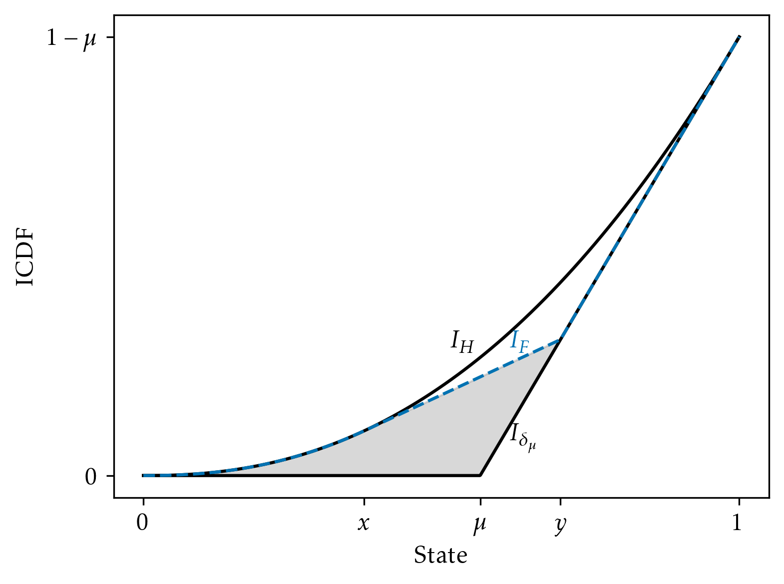
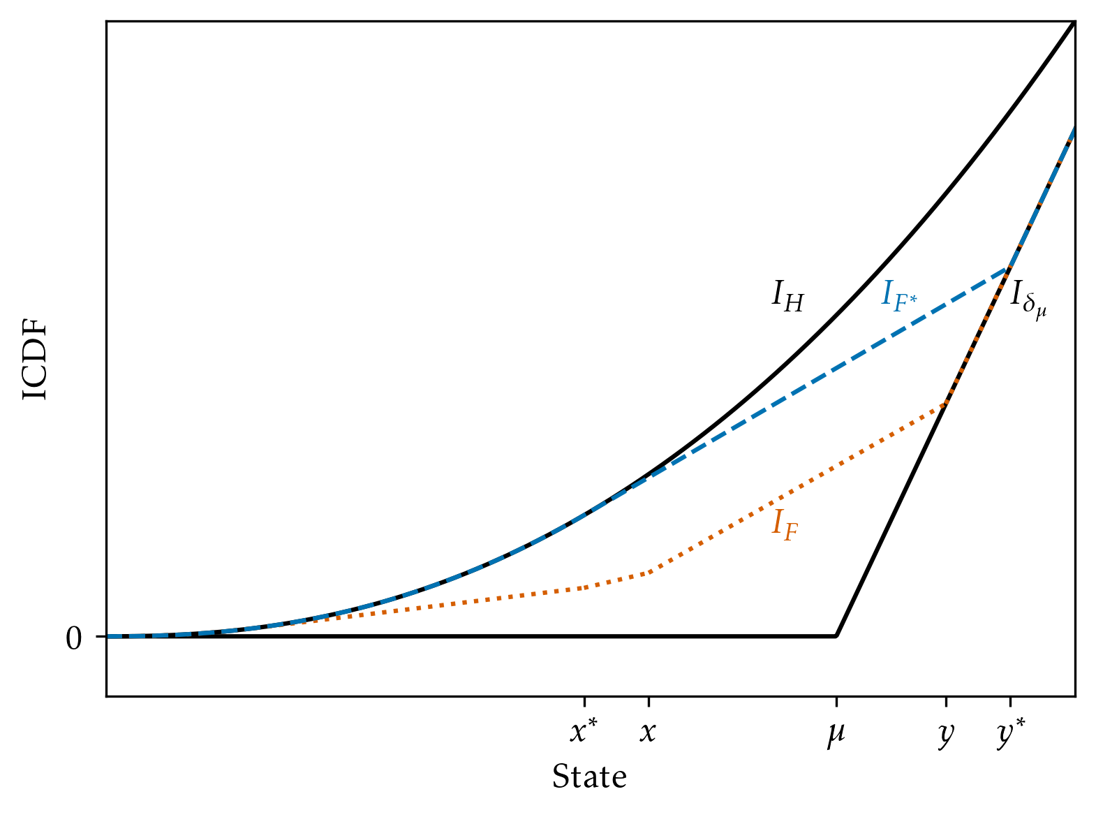
Let $\delta_{\mu}$ be the degenerate (uninformative) experiment, i.e., the Dirac measure on the prior mean $\mu$. Then, we can express $\operatorname*{MPC}(H)$ as the set of CDFs $F$ satisfying $I_{\delta_{\mu}}\leq I_{F}\leq I_{H}$. Figure˜1 depicts the ICDF representation and constraint.

Figure 1: The ICDFs of the prior $H$, the degenerate experiment $\delta_{\mu}$, and an experiment $F$ that pools $H$ above a threshold $x$ to a point $y$, and else coincides with $H$.

Restrictions.

Before the experimenter chooses an experiment, the designer imposes a restriction $\bar{F}\in\operatorname*{MPC}(H)$: given restriction $\bar{F}$, the experimenter must choose an experiment from the set $\operatorname*{MPC}(\bar{F})$ rather than from $\operatorname*{MPC}(H)$. Note, a restriction is an MPS-upper bound on admissible experiments, not an MPS-lower bound: the experimenter can always garble information. We discuss this model of informational restrictions along with real-world analogues at the end of this section. In Figure˜1, if the restriction is $F$, the experimenter can choose among experiments whose ICDFs lie between $I_{F}$ and $I_{\delta_{\mu}}$, as indicated by the shaded area. For example, $F$ is admissible, but $H$ is not.

Incentive-compatibility and optimality.

Given a posterior mean $m$ and outside option $r$, the DM chooses to act ($a=1$) if and only if $m\geq r$. It follows from the experimenter’s state-independent payoffs that the experimenter’s interim expected payoff from inducing a posterior mean $m$ equals $G(m)$. Importantly, this payoff is $S$-shaped (Assumption˜1). The experimenter’s ex-ante payoff from an experiment $F$ equals $\intop\nolimits G(m)\mathop{}\!\mathrm{d}F(m)$.

Given restriction $\bar{F}$, let $\operatorname*{BR}(\bar{F})$ be the set of the experimenter’s best replies:

$$\operatorname*{BR}(\bar{F})=\operatornamewithlimits{argmax}_{F\in\operatorname*{MPC}(\bar{F})}\intop\nolimits G(m)\mathop{}\!\mathrm{d}F(m).$$

An alternative interpretation of $\operatorname*{MPC}(\bar{F})$ is simply the set of all experiments when $\bar{F}$ is the underlying prior distribution of the state. Accordingly, $F\in\operatorname*{BR}(\bar{F})$ means that the experimenter finds $F$ optimal given full delegation and the fictitious prior $\bar{F}$.

We define the set of incentive-compatible experiments as those that are best replies to some restriction.

Definition 1.

An experiment $F\in\operatorname*{MPC}(H)$ is incentive compatible if there exists a restriction $\bar{F}\in\operatorname*{MPC}(H)$ such that $F\in\operatorname*{BR}(\bar{F})$. We denote the set of incentive-compatible experiments by $\mathcal{F}^{\operatorname*{IC}}$.

A useful observation is that an experiment $F$ is incentive compatible if and only if $F\in\operatorname*{BR}(F)$; that is, when $F$ is the imposed restriction, the experimenter finds it optimal not to garble the restriction. To see why, suppose $F\in\operatorname*{BR}(\bar{F})$ for some restriction $\bar{F}$, implying that $F$ is optimal for the experimenter among the admissible experiments $\operatorname*{MPC}(\bar{F})$. Since $F\in\operatorname*{MPC}(\bar{F})$, all mean-preserving contraction of $F$ are admissible too, that is, $\operatorname*{MPC}(F)\subseteq\operatorname*{MPC}(\bar{F})$. Thus, imposing $F$ as a restriction instead of $\bar{F}$ possibly shrinks the set of admissible experiments while $F$ remains admissible. Naturally, $F$ remains optimal among $\operatorname*{MPC}(F)$, implying $F\in\operatorname*{BR}(F)$.

The designer’s utility from an experiment $F$ equals $\intop\nolimits u_{D}(m)\mathop{}\!\mathrm{d}F(m)$. An incentive-compatible experiment is optimal if it maximizes the designer’s utility across the set of incentive-compatible experiments $\mathcal{F}^{\operatorname*{IC}}$. An optimal incentive-compatible experiment exists; see Section˜A.1.

2.1 Examples of Restrictions

We illustrate through several examples how our framework captures various forms of restrictions on real-world information provision. In the examples, we consider the experimenter’s available information and possible communication more explicitly. To do so, we use the language of signals. A signal consists of a measurable space $\mathcal{S}$ and a random variable $\pi\colon[0,1]\times[0,1]\to\mathcal{S}$; here, $\pi(\omega,z)$ represents the signal realization given the state $\omega$ and a uniformly distributed random variable $z$ that is independent of $\omega$. It is apparent how choices of signals and restrictions on them map back to our reduced-form notation in terms of distributions of the posterior means and mean-preserving contractions. For any signal $(\mathcal{S},\pi)$, let $F_{(\mathcal{S},\pi)}$ be the induced distribution of posterior means. Any garbling of $(\mathcal{S},\pi)$ induces a mean-preserving contraction of $F_{(\mathcal{S},\pi)}$.

Restrictions on communication.

Consider a model in which the designer restricts what the experimenter can reveal about the state. Suppose that the designer first chooses a set of signals. Then, the experimenter can choose any signal from or a Blackwell-garbling thereof. With the initial choice of , the designer effectively places an upper bound on what the experimenter can reveal about the state, even if the experimenter can observe the state perfectly. However, the ability to garble any experiment ensures that the experimenter can obfuscate any signal further.

For example, suppose that the state is distributed uniformly on $[0,1]$. A legislator requires a three-category claim structure with $\mathcal{S}=\{i,sg,vg\}$ (innocent, somewhat guilty, and very guilty) and imposes the deterministic map

$$\pi(\omega)=\begin{cases}i,&\text{ if }\omega\in[0,1/3)\\ sg,&\text{ if }\omega\in[1/3,2/3)\\ vg,&\text{ if }\omega\in[2/3,1].\end{cases}$$ (1)

This corresponds to a restriction $\bar{F}=\frac{1}{3}\delta_{1/6}+\frac{1}{3}\delta_{1/2}+\frac{1}{3}\delta_{5/6}$. The prosecutor can however choose to communicate coarser by merging $sg$ and $vg$ into a joint guilty signal $g$. The resulting experiment $F$ would correspond to $F=\frac{1}{3}\delta_{1/6}+\frac{2}{3}\delta_{2/3}$.

Restrictions on measurement.

Consider a model in which the designer restricts what the experimenter can measure about the state. Suppose that the designer can choose to reveal only partial information about the state to the experimenter, that is, the designer chooses a signal $([0,1],\pi)$ in which the signal space coincides with the state space $[0,1]$. The experimenter then chooses an arbitrary signal $(\mathcal{S}^{\prime},\pi^{\prime})$ that defines what the DM will eventually observes. However, the input into the experimenter’s signal is not the realized state $\omega$ but the signal realization that the experimenter receives through the designer’s signal.

For example, a regulator specifies the measurement technology that a producer must use to estimate a product’s safety. Suppose that the underlying state (the product’s safety) $\omega$ is uniformly distributed on $[0,1]$. Then, one restriction is that the measurement technology can only produce binary outcomes $\pi\in\{0,1\}$ (safe or not safe) with $\Pr(\bm{\pi}=1\mid\omega)=\omega$ and $\Pr(\bm{\pi}=0\mid\omega)=1-\omega$. Thus, the regulator’s restriction corresponds to $\bar{F}=\frac{1}{2}\delta_{1/3}+\frac{1}{2}\delta_{2/3}$. The producer can then process these estimated states further. For instance, the producer can hide the test result with probability $1-\alpha$ and truthfully reveal it with probability $\alpha$. This induces the experiment $F=(1-\alpha)\delta_{1/2}+\frac{\alpha}{2}\delta_{1/3}+\frac{\alpha}{2}\delta_{2/3}$.

Attention management.

Consider a sender and receiver with payoffs $u_{S}(m)$ and $u_{R}(m)$ given posterior-mean $m$. The receiver incurs a cost $c(m)$ for “paying attention” to the sender’s information. The receiver may therefore choose to ignore some information, modeled as choosing a mean preserving-contraction $F$ of the sender’s experiment $\bar{F}$. This model can be mapped into our environment by re-interpreting the sender as our designer with $u_{D}=u_{S}$ and the receiver as our experimenter with $G=u_{R}-c$.

Consider an expert, the sender, who writes a research report about a topic that fully reveals the state, $\bar{F}=H$, which is uniformly distributed on $[0,1]$. Then, a journalist, the receiver, decides how much attention to pay to the report. In particular, the journalist chooses to read the report with probability $\alpha$, learning the state $\omega$, and with probability $1-\alpha$, the journalist ignores the report and does not update their belief. The journalist’s experiment is then $F=\alpha H+(1-\alpha)\delta_{1/2}$. The realized attention cost for the journalist is $\alpha\mathbb{E}_{F}[c(\bm{\omega})]+(1-\alpha)c(1/2)$.

Privacy-preserving signals.

Suppose the designer specifies a family $\mathcal{P}$ of events $P$ called privacy sets about which the experimenter’s signal cannot reveal information in the sense of Strack and Yang (2024). Formally, a signal $(\mathcal{S},\pi)$ is privacy preserving given $\mathcal{P}$ if for all $P\in\mathcal{P}$ it holds $\Pr(\bm{\omega}\in P\mid\pi)=\Pr(\bm{\omega}\in P)$ almost surely, and $\mathcal{P}$ is closed with respect to finite intersections. Strack and Yang (2024, Theorem 2) characterize the distributions of posterior means that are induced by privacy-preserving signals. Importantly for us, these distributions are exactly characterized by an MPS-upper bound; that is, given $\mathcal{P}$, there exists a particular cdf $\bar{F}\in\operatorname*{MPC}(H)$ such that an experiment $F$ is privacy preserving if and only if $F\in\operatorname*{MPC}(\bar{F})$. Therefore, in our model, such privacy constraints are captured by imposing $\bar{F}$ as a restriction. Conversely, we show in Section˜6.1 that optimal restrictions can be implemented by a simple class of so-called conditionally privacy-preserving signals.

3 Benchmark: Full Delegation

In this section, we discuss the benchmark in which the designer fully delegates the experiment choice to the experimenter, that is, when $\bar{F}=H$. Hence, there is no restriction in place and the experimenter chooses among all mean-preserving contractions of the prior $H$, $\operatorname*{MPC}(H)$. The results in Kolotilin et al. (2022) imply that upper censorship of the prior is the unique best reply of the experimenter: the experimenter reveals all states below a threshold $x$, and pools all remaining states to an atom $y=\mathbb{E}_{H}[\bm{\omega}\mid\bm{\omega}\geq x]$. The dashed blue experiment $F$ depicted in Figure˜1 is an instance of an upper censorship experiment.

Definition 2.

An experiment $F$ is upper censorship (of the prior $H$) with threshold $x$ and atom $y$ if $F$ coincides with the prior $H$ on the interval $[0,x]$ and assigns mass $1-H(x)$ to the point $y=\mathbb{E}_{H}[\bm{\omega}\mid\bm{\omega}\geq x]$.

We restate the characterization from Kolotilin et al. (2022) of the experimenter’s best reply.

Proposition 1 (Kolotilin et al. (2022)).

There is a unique best reply $F^{\ast}$ to $H$. In particular, $F^{\ast}$ is an upper censorship experiment with a threshold $x^{\ast}$ and an atom $y^{\ast}=\mathbb{E}_{H}[\bm{\omega}\mid\bm{\omega}\geq x^{\ast}]$ satisfying $0<x^{\ast}<r_{0}<y^{\ast}<1$ and

$$G(x^{\ast})+g(y^{\ast})(y^{\ast}-x^{\ast})=G(y^{\ast}).$$ (2)

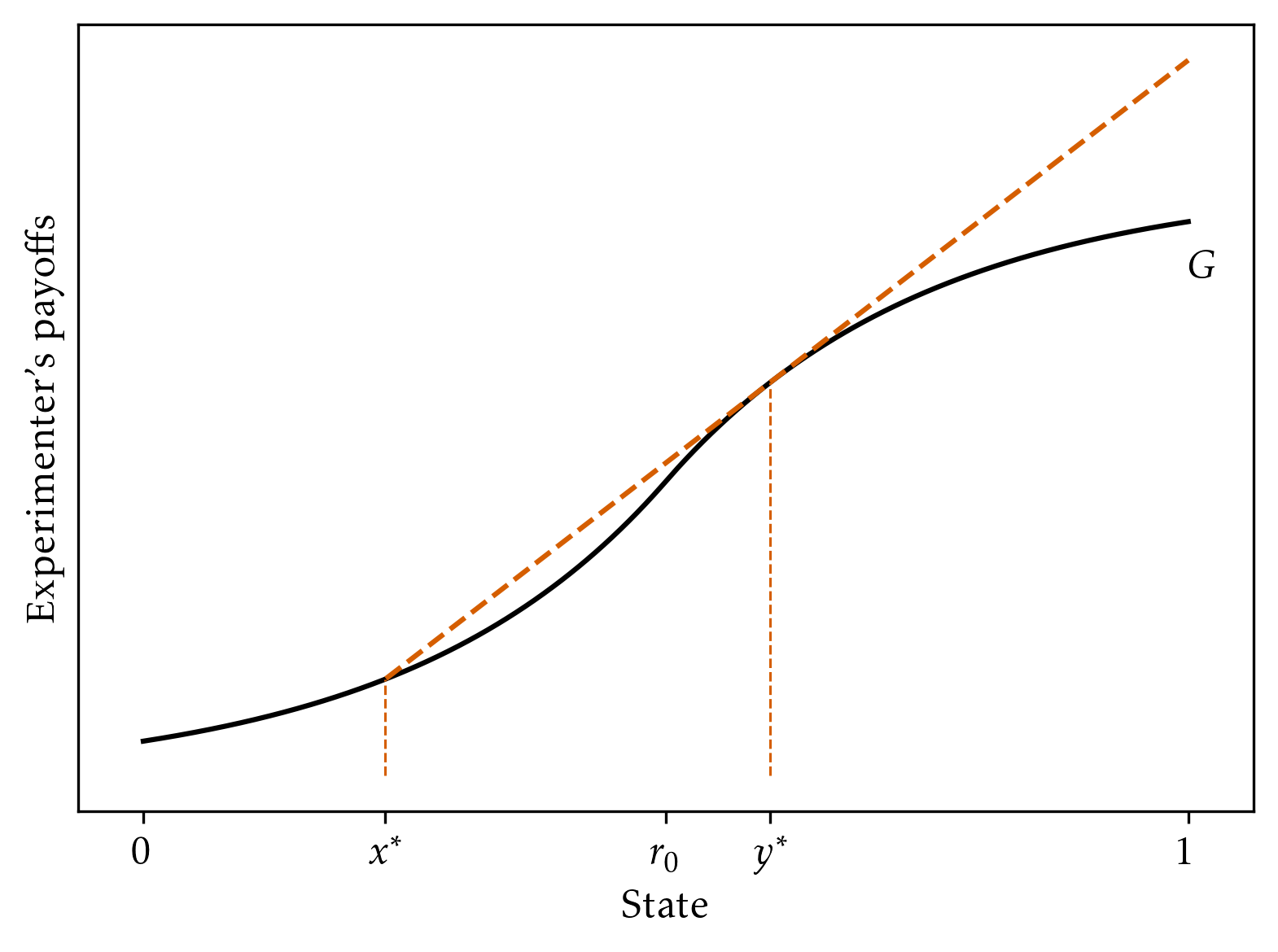
We recall the intuition from Kolotilin et al. (2022). The atom $y^{\ast}$ lies in the concave region of the experimenter’s payoff $G$. Due to this concavity, the experimenter optimally pools some states around $y^{\ast}$ to $y^{\ast}$. As pooling additional states into $y^{\ast}$ raises the probability of the pooling outcome, the experimenter also adds some states from the convex part into the pooling region. Equation˜2 is the first-order condition that characterizes the optimal pooling region, trading off the value of revelation in the convex region against the likelihood of the pooling outcome. Figure˜2 depicts this optimality condition and illustrates the optimal upper censorship experiment.

Figure 2: Equation˜2 defines the optimal upper censorship experiment, illustrated by the red dotted line. The tangent to $G$ at $y^{\ast}$ intersects $G$ at $x^{\ast}$. Since $x^{\ast}<r_{0}$, some states in the convex region of the experimenter’s payoff are also pooled into the high atom $y^{\ast}$.

Importantly, the threshold $x^{\ast}$ is interior: the experimenter reveals a non-trivial interval of states. The interiority of $x^{\ast}$ follows from Assumption˜2. If this assumption fails, the results in Kolotilin et al. (2022) imply that the uninformative experiment $\delta_{\mu}$ is the unique best reply to $H$.

When the designer can pick a restriction, Assumption˜2 remains necessary for information transmission. Trivially, $\delta_{\mu}$ is admissible under all restrictions and imposing a restriction only shrinks the set of experiments from which the experimenter can choose. Thus, if the experimenter’s best reply to the prior $H$ is unique and uninformative—i.e. $\delta_{\mu}=\operatorname*{BR}(H)$—, then $\delta_{\mu}$ is also the unique best reply to all restrictions. For this reason, we maintain Assumption˜2.

The optimal upper censorship experiment provides the relevant benchmark for the designer. The designer can always guarantee the payoff from the optimal censorship experiment by full delegation, not restricting the set of admissible experiments. However, under upper censorship a significant set of states is pooled into a point and, hence, substantial information is lost. We next study which alternative experiments the designer can induce by introducing non-trivial delegation sets.

4 Maximal Incentive-Compatible Experiments

In this section, we first show that it suffices to consider a subset of incentive-compatible experiments that we call maximal. Our first main result characterizes the entire set of maximal incentive-compatible experiments.

4.1 Motivation and Definition

Incentive-compatible experiments represent all experiments that the designer can implement with some delegation set. However, some incentive-compatible experiments are clearly suboptimal. For example, the uninformative experiment $\delta_{\mu}$ is straightforwardly incentive-compatible: when the designer imposes $\delta_{\mu}$ as a restriction, the delegation set contains only the uninformative experiment $\delta_{\mu}$ and the experimenter can only choose $\delta_{\mu}$. However, the designer never finds it optimal to implement $\delta_{\mu}$ since $\delta_{\mu}$ is strictly less informative than the full delegation outcome $F^{\ast}$, and since the designer has strictly convex payoffs.

This observation suggests to refine the candidate set of optimal experiments by considering only those incentive-compatible experiments that are not mean-preserving contractions of other incentive-compatible experiments. We next formalize this refinement and show that it is indeed without loss for optimality.

Definition 3.

An incentive-compatible experiment $F$ is maximal (MIC) if there does not exist an incentive-compatible experiment $\tilde{F}$ of which $F$ is a proper mean-preserving contraction; that is, there does not exist an incentive-compatible experiment $\tilde{F}$ such that $F\in\operatorname*{MPC}(\tilde{F})$ and $\tilde{F}\notin\operatorname*{MPC}(F)$.

Economically, the set of MIC experiments is the relevant boundary of what the designer can implement. An MIC experiment represents a restriction that the experimenter has no incentive to garble, whereas the experimenter would garble every strictly more informative restriction.

The full delegation outcome $F^{\ast}$ is an example of an MIC experiment. To see why, let $F$ be an incentive-compatible experiment of which $F^{\ast}$ is a mean-preserving contraction. On the one hand, the assumption that $F$ is incentive compatible and a mean-preserving spread of $F^{\ast}$ implies that the experimenter weakly prefers $F$ to $F^{\ast}$ when $F$ is given as a restriction. On the other hand, Proposition˜1 asserts that the experimenter strictly prefers $F^{\ast}$ over all other experiments. Hence, the experiments $F$ and $F^{\ast}$ must be identical, implying that $F^{\ast}$ is MIC.

The following lemma justifies restricting attention to MIC experiments.

Lemma 1.

For all incentive-compatible experiments $F$ there exists a maximal incentive-compatible experiment $\hat{F}$ that is a mean-preserving spread of $F$.

Lemma˜1 implies that it is without loss to focus on MIC experiments when searching for restrictions delivering optimal delegation sets. The MIC experiment $\hat{F}$ is incentive compatible. Hence, the experimenter will optimally choose the experiment $\hat{F}$ when the designer’s restriction is $\hat{F}$. Further, since $\hat{F}$ is a mean-preserving spread of $F$, the designer and DM, who have convex posterior-mean payoffs, prefer $\hat{F}$ over $F$.

To gain intuition for the existence argument, suppose $F$ is not MIC. By definition, this means there is an incentive-compatible experiment that is a mean-preserving spread of $F$. If this experiment is also not MIC, there is a further incentive compatible mean-preserving spread, and so on. A compactness argument shows that this reasoning delivers an MIC experiment $\hat{F}$ that is a mean-preserving spread of $F$.

The notion and optimality of MIC experiments highlight how the designer may potentially benefit from imposing a restriction despite having a preference for information. All MIC experiments are incomparable to one another, by definition of maximality. Since MIC experiments are without loss, the designer thus trades-off informativeness about different regions of the state space when choosing among MIC experiments. In particular, since the full delegation outcome $F^{\ast}$ is also an MIC experiment, the candidate set of experiments is incomparable to $F^{\ast}$.

Remark.

The experiment $\hat{F}$ in Lemma˜1 Pareto dominates $F$. As already noted, the DM and the designer with convex payoffs prefer $\hat{F}$ to $F$ since $F\in\operatorname*{MPC}(\hat{F})$. Turning to the experimenter, incentive compatibility of $\hat{F}$ implies that the experimenter finds $\hat{F}$ optimal when $\hat{F}$ is given as a restriction. In particular, since $F\in\operatorname*{MPC}(\hat{F})$, the experimenter prefers $\hat{F}$ to $F$.

4.2 Double Censorship

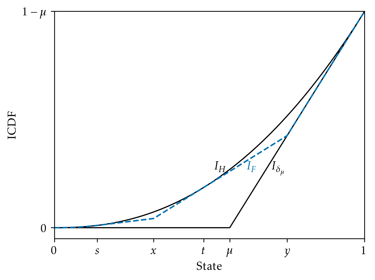
In our main characterization result, we show that all MIC experiments take the form of double censorship experiments. We introduce them formally in the definition below. Intuitively, a double-censorship experiment divides the state space into three intervals: a fully revealing interval, an intermediate pooling interval, and a high pooling interval. Figure˜3 depicts the ICDF of a double-censorship experiment.

Definition 4.

An experiment $F$ is double censorship with thresholds $(s,t)$ and atoms $(x,y)$ if $s\leq t$ and $x=\mathbb{E}_{H}[\bm{\omega}\mid\bm{\omega}\in[s,t]]$ and $y=\mathbb{E}_{H}[\bm{\omega}\mid\bm{\omega}\in[t,1]]$ and

$$\forall m\in[0,1],\quad F(m)=\begin{cases}H(m)\quad&\mbox{if }m\in[0,s),\\ H(s)\quad&\mbox{if }m\in[s,x),\\ H(t)\quad&\mbox{if }m\in[x,y),\\ 1\quad&\mbox{if }m\in[y,1].\end{cases}$$

Each upper censorship experiment, including the full-delegation outcome $F^{\ast}$, is a special double censorship experiment with $s=x=t$, and such that all states below $x$ are fully revealed while all states above $x$ are pooled to $y=\mathbb{E}_{H}[\bm{\omega}\mid\bm{\omega}\in[x,1]]$.

Figure 3: The ICDF of double censorship $F$ with thresholds $(s,t)$ and atoms $(x,y)$.

4.3 Characterization

Our first main result shows that all MIC experiments take the form of double censorship. To do so, we introduce the set $P$, which relates the two atoms of a double censorship experiment to each other through a tangency condition similar to the one in Proposition˜1 and depicted in Figure˜2. We will see that this tangency condition characterizes incentive-compatibility of double censorship experiments. Formally, let

$$P=\{(x,y)\colon 0\leq x\leq r_{0}\leq y\leq 1\mbox{ and }G(x)+g(y)(y-x)=G(y)\}.$$ (3)

Theorem 1.

An experiment $F$ is MIC if and only if $F$ is a double censorship experiment with thresholds $(s,t)$ and atoms $(x,y)$ satisfying

$$(x,y)\in P\quad\mbox{and}\quad s\leq x^{\ast}\leq t\quad\mbox{and}\quad 0<x<y<1,$$

where $x^{\ast}$ denotes the threshold of the upper censorship experiment under full delegation.

Theorem˜1 shows that double censorship experiments are the only candidates for MIC experiments. MIC experiments are characterized by interpretable properties of the thresholds $s$ and $t$, and the atoms $x$ and $y$. The first property, $(x,y)\in P$, characterizes incentive-compatibility for double censorship experiments, as we explain in more detail in the discussion of the proof. The second property, $s\leq x^{\ast}\leq t$, reflects maximality and highlights how a given MIC experiment $F$ compares to the full-delegation outcome $F^{\ast}$. On the one hand, the pooling region $[t,1]$ is contained in the full-delegation pooling region $[x^{\ast},1]$. On the other hand, there is a new pooling region $[s,t]$ vis-à-vis full revelation of states below $x^{\ast}$ under full delegation. Finally, the inequalities $0<x<y<1$ assert that $x$ and $y$ are indeed distinct atoms and imply that $F$ is non-degenerate.

Theorem˜1 shows how each given MIC experiment compares to the full delegation outcome $F^{\ast}$ (itself an MIC experiment). More generally, choosing among MIC experiments entails trading off the experiment’s informational content about different regions of the state space. We can express this trade-off via a total order:

Corollary 1.

For all two MIC double censorship experiments with respective parameters $(s,t,x,y)$ and $(s^{\prime},t^{\prime},x^{\prime},y^{\prime})$, if $y^{\prime}<y$, then $[s^{\prime},t^{\prime}]\subsetneq[s,t]$ and $[t,1]\subsetneq[t^{\prime},1]$ and $x<x^{\prime}$.

Thus, the designer can shrink the upper pooling region $[t,1]$ (an informational gain) only by expanding the lower pooling region $[s,t]$ (an informational loss). This trade-off is driven by the need to maintain the constraint $(x,y)\in P$ that reflects incentive compatibility. Corollary˜1 implies that MIC experiments are a one-parameter family indexed and ordered by the top atom $y$. Given $y$, we can compute $(s,t,x)$ using the condition $(x,y)\in P$ from Theorem˜1 and the definition of $x$ and $y$ as conditional expectations for double censorship experiments.

4.4 Sketch of the Proof

In the following, we outline the proof of Theorem˜1, focusing on the characterization of an arbitrary MIC experiment as a double censorship experiment. In the appendix, we also prove the other direction that all double censorship experiments with the properties in Theorem˜1 are MIC experiments.

First, we characterize incentive-compatible experiments in our environment using the price-theoretic approach of Dworczak and Martini (2019).

Lemma 2.

An experiment $F$ is IC if and only if there exists a convex, continuous function $p\colon[0,1]\to\mathbb{R}$ such that $p\geq G$ and $\operatorname*{supp}F\subseteq\{m\in[0,1]\colon p(m)=G(m)\}$.

Proof of Lemma˜2.

Dworczak and Martini (2019, Corollary 1) provide the following necessary and sufficient condition for an experiment $F$ to be optimal in an unconstrained persuasion problem when the prior is some distribution $\bar{F}$: Given a prior $\bar{F}$ and $F\in\operatorname*{MPC}(\bar{F})$, it holds $F\in\operatorname*{BR}(\bar{F})$ if and only if there exists a convex, continuous function $p\colon[0,1]\to\mathbb{R}$ such that $p\geq G$ and $\operatorname*{supp}F\subseteq\{m\in[0,1]\colon p(m)=G(m)\}$ and $\intop\nolimits p(m)\mathop{}\!\mathrm{d}F(m)=\intop\nolimits p(m)\mathop{}\!\mathrm{d}\bar{F}(m)$.

Our lemma follows from this result and recalling that an experiment $F$ is incentive-compatible if and only if $F$ is a best reply to itself, that is, if $F\in\operatorname*{BR}(F)$. Thus, $F$ would be optimal in the full-delegation problem if $F$ was the prior. Indeed, if $F=\bar{F}$, then the integral condition $\intop\nolimits p(m)\mathop{}\!\mathrm{d}F(m)=\intop\nolimits p(m)\mathop{}\!\mathrm{d}\bar{F}(m)$ trivially holds. ∎

To further characterize incentive-compatible experiments, we combine Lemma˜2 with $S$-shapedness of the experimenter’s payoff.

Lemma 3.

A non-degenerate experiment $F$ is incentive-compatible if and only if there exist $(x,y)\in P$ such that $F$ assigns no mass to the set $(x,y)\cup(y,1]$.

To gain intuition, suppose $F$ is an incentive-compatible experiment. Then, $F$ cannot assign mass to multiple states in the concave part $[r_{0},1]$ of the experimenter’s payoff $G$ since the experimenter would strictly prefer to pool such states. Thus, there is at most one point $y$ in support of $F$ above $r_{0}$. In fact, as discussed in the context of full delegation in Section˜3, the experimenter would also pool some states just below the inflection point $r_{0}$ to shift more probability mass to the pooling outcome. The point $x<r_{0}$ represents the cutoff value where the experimenter finds it optimal to pool no further, as reflected in the condition $G(x)+g(y)(y-x)=G(y)$ that defines the set $P$ (recall (3)). We conclude that $F$ cannot assign mass to $(x,y)\cup(y,1]$. Note, however, that we cannot yet conclude that, as in double censorship, $y$ is obtained by pooling the prior above some threshold, or that $x$ or $y$ are even in the support of $F$.

Lemma˜3 shows that incentive-compatibility is fully characterized by regions of the state space on which an experiment does not assign any mass. Thus, any MIC experiment should reveal as much information as possible while respecting these forbidden regions. We next show how double censorship emerges from combining incentive-compatibility with maximality considerations. To that end, we first prove that the set $P$, which characterizes the forbidden regions, is ordered by set inclusion.

Lemma 4.

If $(x,y)\in P$ and $(x^{\prime},y^{\prime})\in P$, then $[x,y]\subseteq[x^{\prime},y^{\prime}]$ or $[x^{\prime},y^{\prime}]\subseteq[x,y]$.

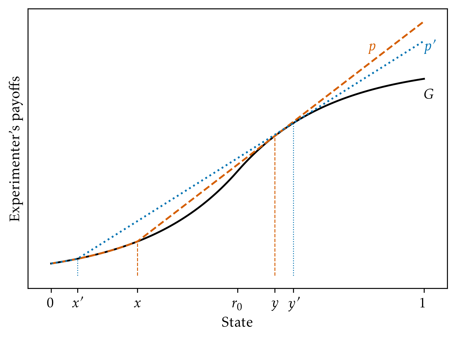
This lemma directly follows from the $S$-shapedness of $G$, as illustrated in Figure˜4. Whenever there is a feasible $(x,y)$-combination, that is, one that satisfies (3), the tangent of the experimenter’s value at $y$ has to intersect the experimenter’s value at $x$. As $y\geq r_{0}$, the point $y$ lies in the concave part of the experimenter’s value. Now, consider a marginal increase in $y$. By concavity, the tangent of the experimenter’s value becomes flatter. Hence, the intersection with the experimenter’s value must occur at a lower value. It follows that the intervals $[x,y]$ defined by the elements of the set $P$ are nested.

Figure 4: The order of the set $P$. For a higher value of $y$, the slope of $y$ is lower, meaning the tangent to $G$ at $y$ intersects $G$ below $r_{0}$ at a lower point $x$.

Next, we derive the remaining properties of the characterization of MIC experiments that result from maximality. Consider an arbitrary MIC experiment $F$. Incentive-compatibility implies, by Lemma˜3, that $F$ does not allocate any mass to $[x,y)\cup(y,1]$, which implies that the ICDF $I_{F}$ of the experiment $F$ is affine on $[x,y]$ and $[y,1]$. Maximality implies then that $F$ is as informative as possible subject to not assigning any mass to the forbidden regions. Moreover, due to Lemma˜4, we only have to distinguish two cases for how any MIC experiment $F$ relates to the full-delegation outcome $F^{\ast}$: the experiment $F$ is such that $[x,y]\subseteq[x^{\ast},y^{\ast}]$ or it is such that $[x^{\ast},y^{\ast}]\subseteq[x,y]$.

First, suppose $[x,y]\subseteq[x^{\ast},y^{\ast}]$. In this case, we show that $F$ must be an MPC of the full-delegation outcome $F^{\ast}$ and therefore not maximal unless $F=F^{\ast}$. We illustrate graphically in Figure˜5(a). As the experiments $F$ and $F^{\ast}$ assign no mass to $[y,1]$ and $[y^{\ast},1]$, respectively, their ICDFs both hit the ICDF of the uninformative experiment at $y$ and $y^{\ast}$, respectively. In particular, since $y^{\ast}\geq y$, we find $I_{F}(y^{\ast})=I_{F^{\ast}}(y^{\ast})$. In this sense, the experiment $F$ pools weakly more states at the top than $F^{\ast}$. Moreover, $I_{F}$ lies weakly below $I_{F^{\ast}}$ on $[0,x^{\ast}]$ since the full-delegation $F^{\ast}$ outcome fully reveals all states in this region. Therefore, $F^{\ast}$ is weakly more informative at the bottom as well. Finally, note that $I_{F^{\ast}}$ is affine on $[x^{\ast},y^{\ast}]$, while $I_{F}$ is convex. Since $I_{F}(x^{\ast})\leq I_{F^{\ast}}(x^{\ast})$ and $I_{F}(y^{\ast})=I_{F^{\ast}}(y^{\ast})$, we obtain $I_{F}(m)\leq I_{F^{\ast}}(m)$ for all $m\in[x^{\ast},y^{\ast}]$. Summarizing, we find that $I_{F}$ lies below $I_{F^{\ast}}$ on all of $[0,1]$, implying that $F$ is an MPC of $F^{\ast}$. The experiment $F^{\ast}$ is incentive-compatible. Thus, for $F$ to be maximal, we must have $F=F^{\ast}$, implying that $F$ is upper censorship, which is a special case of double censorship.

(a) An incentive-compatible experiment $F$ that is an MPC of $F^{\ast}$.

(b) An incentive-compatible experiment $F$ and a double censorship experiment that is an MPS of $F$.

Figure 5: Characterization of MIC experiments. For readability, the horizontal axes are truncated at the top.

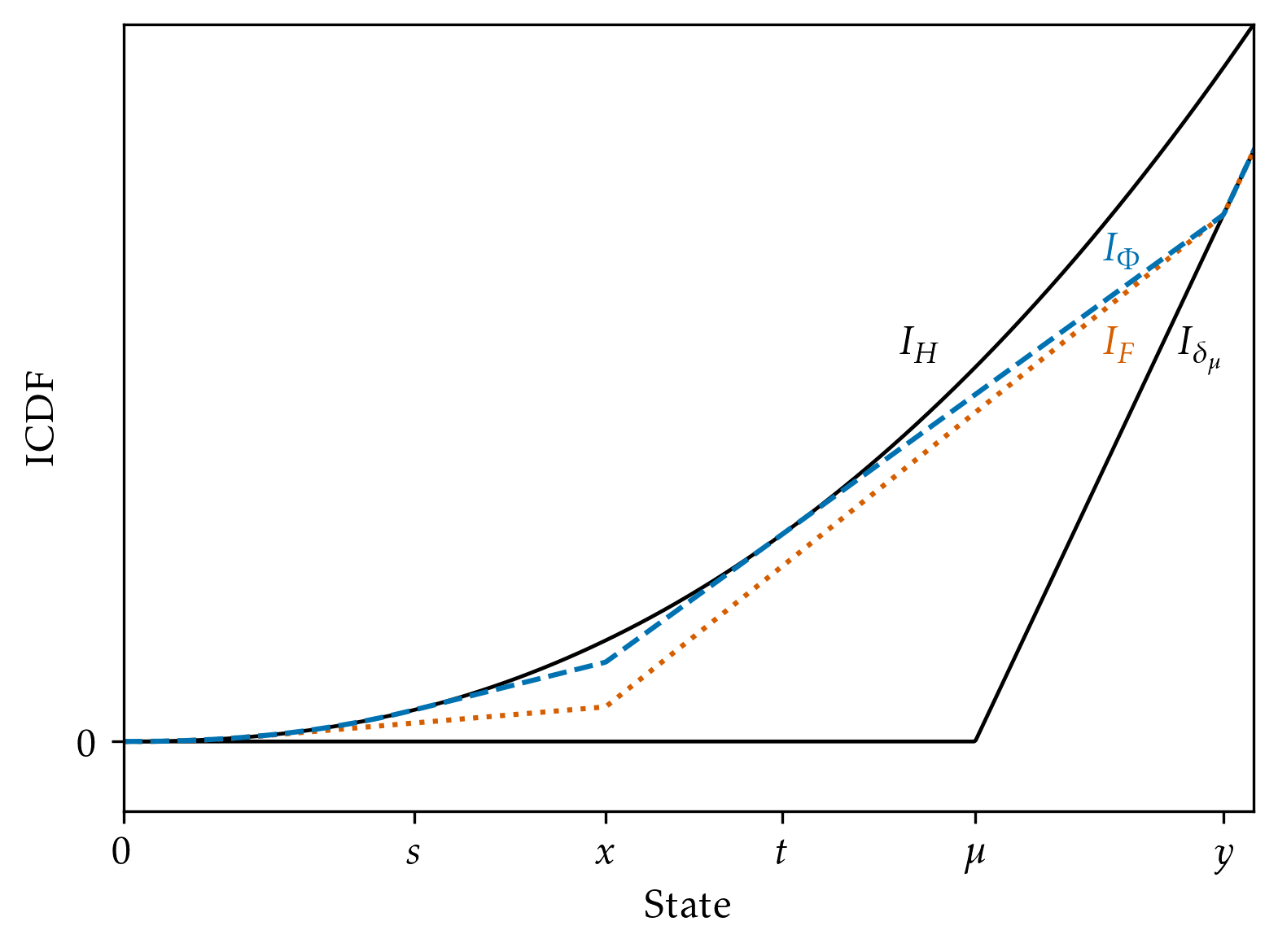
Second, suppose $[x^{\ast},y^{\ast}]\subseteq[x,y]$. We illustrate this case graphically in Figure˜5(b). In this case, $I_{F}$ hits the ICDF of the uninformative experiment at $y\geq y^{\ast}$ and, hence, after $I_{F^{\ast}}$. It follows from incentive-compatibility that $I_{F}$ is affine on $[x,y]$ and coincides with $I_{H}$ at most once on this interval. For the purpose of this sketch, suppose $I_{F}$ lies strictly below $I_{H}$ on $[x,y]$. In this case, we can obtain a new experiment by rotating the affine segment of $I_{F}$ on $[x,y]$ clockwise, while anchoring it $I_{F}(y)$, until it is tangent to $I_{H}$ at some point $t$. Then, we can find a point $s$ such that the tangent to $I_{H}$ at $s$ intersects the new affine segment at $x$. Finally, we let reveal all states below $s$. In the proof, we show that $[x^{\ast},y^{\ast}]\subseteq[x,y]$ guarantees the existence of such points $s$ and $t$. The constructed is incentive-compatible, a mean-preserving spread of $F$, and a double-censorship experiment. Incentive-compatibility follows from Lemma˜3 as does not allocate mass to the set $[x,y)\cup(y,1]$, while $\Phi\in\operatorname*{MPS}(F)$ follows since $I\geq I_{F}$. Hence, for $F$ to be maximal, we must have $F=\Phi$, implying that $F$ is double censorship.

5 Optimal Delegation

5.1 Full delegation is not optimal

We now revisit the designer’s problem that is at the core of our environment. Anticipating the persuasion motive of the experimenter, can the designer gain from restricting the set of experiments available to the experimenter even though the designer has a preference for informative experiments? To answer this, Lemma˜1 implies that it suffices to consider restrictions that are MIC experiments, i.e. the experimenter has no incentive to garble the restriction but would garble any more informative restriction. We now apply our characterization of MIC experiments as double censorship experiments. The following theorem is our second main result.

Theorem 2.

The full delegation outcome $F^{\ast}$ is not optimal.

We prove Theorem˜2 using a local perturbation argument at the full-delegation solution. Recall that the family of MIC experiments is a one-dimensional family parametrized by the atom $y$ in the top pooling interval (Corollary˜1). Moreover, full delegation leads to the upper censorship experiment with $y=y^{\ast}$ and $s=t=x^{\ast}$. Denote by $U_{D}(y)$ the designer’s value from choosing the double censorship experiment with $y$ as restriction. Due to Corollary˜1, $y\geq y^{\ast}$. Hence, we consider the right-derivative of $U_{D}(y)$ and evaluate it at $y=y^{\ast}$. After simplifications, we obtain

$$\mathopen{}\mathclose{{\left(u_{D}^{\prime}(y^{\ast})-\frac{u_{D}(y^{\ast})-u_{D}(x^{\ast})}{y^{\ast}-x^{\ast}}}}\right)(1-H(x^{\ast}))>0,$$ (4)

which is strictly positive since $u_{D}$ is strictly convex and $x^{\ast}<y^{\ast}$.

To interpret this derivative, consider first the following hypothetical scenario: the designer is presented with a binary experiment with support $\{x^{\ast},y^{\ast}\}$ and mean $\mu$, and can costlessly perturb the support subject to the mean constraint. The derivative (4) is precisely the change in the designer’s when increasing $y^{\ast}$ marginally while holding $x^{\ast}$ fixed and adjusting the probability of the realization $y^{\ast}$ to satisfy the mean constraint. The term $u_{D}^{\prime}(y^{\ast})$ reflects the marginal increase in the value of the atom $y^{\ast}$, and the term $\frac{u_{D}(y^{\ast})-u_{D}(x^{\ast})}{y^{\ast}-x^{\ast}}$ reflects the mass that is shifted from $y^{\ast}$ to $x^{\ast}$ to maintain the mean. The designer gains from this perturbation as increasing $y^{\ast}$ while fixing $x^{\ast}$ makes the binary experiment more informative.

In our actual model, the designer cannot freely pick the experiment but must additionally satisfy incentive-compatibility. To achieve this, the designer introduces the double censorship thresholds $s$ and $t$. Since the states in the interval $[s,x^{\ast}]$ are now pooled rather than being revealed as in the full-delegation outcome, there is a cost to the perturbation. Importantly, this cost is of second order since the lower threshold $s$ for a given small perturbation remains close to $x^{\ast}$ and, hence, is an order of magnitude smaller than $y^{\ast}-x^{\ast}$ for small perturbations. Formally, this cost is

$$\intop\nolimits_{[s,x^{\ast}]}(u_{D}(x^{\ast})-u_{D}(m))\mathop{}\!\mathrm{d}H(m)$$ (5)

reflecting the informational loss from pooling states to $x^{\ast}$ instead of revealing them. For $s$ close to $x^{\ast}$, this integral is an order of magnitude smaller than the gain reflected in (4).

Remark.

There exists a solution to the designer’s problem, and it is attained by an incentive-compatible double censorship experiment. Viewed as a best reply to itself, this experiment is a fictitious prior with two atoms. Theorem˜2 does not apply to this fictitious prior since the theorem assumes an absolutely continuous prior.

5.2 A Parametric Example

To illustrate our results, we consider a parametrized example. Suppose that the state is uniformly distributed on the unit interval, that is, $H(\omega)=\omega$, and that the outside option distribution is a $Beta(2,2)$ distribution, that is, $G(r)=3r^{2}-2r^{3}$ and $g(r)=6r(1-r)$ with $r_{0}=1/2$. The designer’s and the DM’s payoffs coincide.

Full-delegation benchmark.

First, we consider the full-delegation benchmark, that is, the persuasion solution. By Proposition˜1, the optimal experiment will be upper censorship (with cutoff $x^{\ast}$ and top atom $y^{\ast}=\mathbb{E}[\omega\mid\omega\geq x^{\ast}]$) and determined through the tangency condition. Due to the uniform assumption, we obtain for the top atom $y^{\ast}=(x^{\ast}+1)/2$ (and equivalently $x^{\ast}=2y^{\ast}-1$). Applying the tangency condition (2) yields the optimal upper censorship experiment:

$$x^{\ast}=\frac{1}{4},\quad y^{\ast}=\frac{5}{8}.$$

MIC experiments.

By Theorem˜1, we can restrict attention to double censorship experiments. With our parametric assumptions, we obtain that for a given top atom $y$, the double-censorship experiment is characterized by

$$x(y)=\frac{3}{2}-2y,\quad t(y)=2y-1,\quad s(y)=4-6y$$

as long as the solution is feasible (i.e., $x(y)\leq x^{\ast}$, $0<x<y<1$, and $s\geq 0$). Thus, we can characterize the set of implementable top atoms as the constraint

$$y\in\mathopen{}\mathclose{{\left[\frac{5}{8},\frac{2}{3}}}\right].$$

Optimal delegation.

For any feasible double-censorship experiment with top atom $y$, the designer’s (and DM’s) ex-ante payoff is

$$U_{D}(y)= \intop\nolimits_{0}^{s(y)}\intop\nolimits_{0}^{\omega}(\omega-r)dG(r)\mathop{}\!\mathrm{d}H(\omega)$$

$$+\mathopen{}\mathclose{{\left(H(t(y))-H(s(y))}}\right)\intop\nolimits_{0}^{x(y)}(x(y)-r)\mathop{}\!\mathrm{d}G(r)$$

$$+(1-H(t(y)))\intop\nolimits_{0}^{y}(y-r)\mathop{}\!\mathrm{d}G(r).$$

Applying the expressions for $s(y),x(y)$ and $t(y)$, we obtain that $U_{D}(y)$ is strictly increasing on the feasible range of $y$. Hence, the optimal restriction is $y^{\operatorname*{opt}}=2/3$ and the corresponding optimal double-censorship experiment is characterized by

$$s^{\operatorname*{opt}}=0,\quad x^{\operatorname*{opt}}=\frac{1}{6},\quad t^{\operatorname*{opt}}=\frac{1}{3},\quad y^{\operatorname*{opt}}=\frac{2}{3}.$$

The optimal delegation of information provision induces simple information provision endogenously: a binary signal whether the state is above or below a threshold of $t^{\operatorname*{opt}}=1/3$ is the optimal experiment.

6 Discussion

This section discusses further implications of maximal incentive-compatibility for $S$-shaped experimenter payoffs, how the MIC perspective extends beyond the $S$‑shaped benchmark, and the connection between our problem and the extreme-point approach in the information design literature.

6.1 Further Implications

We begin with two useful observations about optimal restrictions.

Implementation.

Our characterization of optimal restrictions as MIC experiments reveals that the designer can implement an optimal delegation set with a simple restriction. This restriction is obtained from the prior $H$ by pooling all states in the intermediate pooling region and revealing all other states. The experimenter best replies to this restriction by also pooling states above the upper threshold. The following corollary formalizes this observations.

Corollary 2.

If $F$ is MIC double censorship with parameters $(s,t,x,y)$, then $F$ is a best reply to the restriction $\bar{F}$ that is obtained by pooling $H$ on $[s,t]$ to $x$ and otherwise revealing the state.

In Section˜2.1, we saw how privacy-preserving signals (Strack and Yang (2024)) can be regarded as restrictions in our model. We now use Corollary˜2 to explain how MIC experiments are implementable via conditionally privacy-preserving signals, as defined by Strack and Yang. Given a random variable $\xi\colon[0,1]\to\Xi$ (for some measurable set ) and a family $\mathcal{P}$ of Borel subsets of $[0,1]$, say a signal $(\mathcal{S},\pi)$ is conditionally privacy-preserving if for all $P\in\mathcal{P}$ it holds $\Pr(\bm{\omega}\in P\mid\xi,\pi)=\Pr(\bm{\omega}\in P\mid\xi)$ almost surely.

Now fix any MIC double censorship experiment $F$ with thresholds $s$ and $t$. Let $\xi$ be the binary random variable that reveals whether the state lies in the interval $[s,t]$, i.e. $\xi=\bm{1}_{[s,t]}$. Let $\mathcal{P}$ be the family of all Borel subsets of $[s,t]$. Conditional on $\xi=0$—i.e. $\omega\notin[s,t]$—, the privacy constraint holds trivially, since the probability of the event $\{\omega\in P\}$ equals $0$ for all subsets $P$ of $[s,t]$, irrespective of any additional information. Conversely, if $\xi=1$—i.e. $\omega\in[s,t]$—, the privacy constraint requires any signal to reveal no additional information. Therefore, the conditionally privacy-preserving signals are exactly those signals that are Blackwell-less informative than the signal that reveals $\omega$ whenever $\omega$ is outside $[s,t]$ and, otherwise, only reveals that $\omega$ is in $[s,t]$. Corollary˜2 implies that imposing this signal as a restriction (or, more precisely, its distribution of posterior means) yields the given MIC experiment $F$ as a best reply.

Welfare-optimal delegation.

While we took the extreme stance that designer’s preferences are strictly convex, our key insights extend to a designer who maximizes a weighted sum of the DM’s and the experimenter’s utility (which may lead to non-convex posterior-mean payoffs for the designer).

Given a posterior mean $m$, the DM’s interim expected payoff equals $\intop\nolimits_{0}^{1}\max\{m-r,0\}\mathop{}\!\mathrm{d}G(r)$ for all $m\in[0,1]$. Integrating by parts, the DM’s payoff is given by $I_{G}(m)=\intop\nolimits_{0}^{m}G(r)\mathop{}\!\mathrm{d}r$; in particular, the DM’s payoff is strictly convex. The experimenter’s payoff is $G(m)$, as before. Thus, the designer’s payoff is given by $u_{D}(m)=\lambda I_{G}(m)+(1-\lambda)G(m)$, for some weight $\lambda\in[0,1]$ on the DM’s payoffs.

For such a designer, MIC experiments remain without loss. Indeed, in Section˜4.1 we noted that for every incentive-compatible experiment there exists a Pareto-dominating experiment that is MIC.

Next, the characterization of MIC experiments is unchanged, being entirely independent of the designer’s preferences.

Finally, the designer still finds full delegation suboptimal provided the designer assigns a non-zero weight $\lambda$ to the DM. To see this, recall the derivative (4) that we derived via a perturbation argument:

$$\mathopen{}\mathclose{{\left(u_{D}^{\prime}(y^{\ast})-\frac{u_{D}(y^{\ast})-u_{D}(x^{\ast})}{y^{\ast}-x^{\ast}}}}\right)\mathopen{}\mathclose{{\left(1-H(x^{\ast})}}\right).$$

From the characterization of the full delegation outcome, we know $g(y^{\ast})=\frac{G(y^{\ast})-G(x^{\ast})}{y^{\ast}-x^{\ast}}$, reflecting the optimal size of the full delegation pooling region from the experimenter’s perspective. Thus, the derivative from the perturbation simplifies to:

$$\lambda\mathopen{}\mathclose{{\left(G(y^{\ast})-\frac{I_{G}(y^{\ast})-I_{G}(x^{\ast})}{y^{\ast}-x^{\ast}}}}\right)\mathopen{}\mathclose{{\left(1-H(x^{\ast})}}\right).$$

This derivative is strictly positive since the DM’s payoff $I_{G}$ is strictly convex.

6.2 Profitable Restrictions Beyond S-shaped Persuasion

In this subsection, we investigate whether the designer can benefit from imposing a restriction when the experimenter’s payoff $G$ (i.e. the outside option distribution) is not necessarily $S$-shaped. Equivalently, under which conditions is full delegation suboptimal? We argue that two conditions are important for the profitability of restrictions and we formalize the discussion in Appendix˜B. First, the experimenter has locally strict curvature preferences: $G$ is locally strictly convex or strictly concave, and satisfies a technical smoothness condition. Second, the full delegation outcome admits incomplete full revelation: under full delegation, the experimenter fully reveals a non-trivial interval of states, but does not reveal all states.

We begin with two examples to demonstrate the importance of both conditions. We then describe how to generalize the insights from these examples. In this discussion, the definitions of incentive compatibility and optimality are as in the baseline model.

Uninformed DM.

Suppose the DM has no private information: the outside option distribution $G$ is a step function with step at $r_{0}$. In particular, the DM does not have locally strict preferences, being indifferent between revealing and obfuscating the states within the subintervals below and above $r_{0}$, respectively.

In this example, the experimenter maximizes the probability of drawing a posterior mean above $r_{0}$. If $\mu>r_{0}$, the experimenter can induce the DM to take action with probability one regardless of the restriction by choosing the experiment $\delta_{\mu}$; it is then easy to see that the designer cannot gain by imposing a restriction. If $\mu\leq r_{0}$, then, for an arbitrary restriction $\bar{F}$ and best reply $F$, the largest point in the support of $F$ is at most $r_{0}$. This implies that $F$ is an MPC of the experiment that reveals all states up to a threshold $s$ and pools the rest to $r_{0}$ (i.e. $r_{0}=\mathbb{E}_{H}[\bm{\omega}\mid\bm{\omega}\in[s,1]]$, which is feasible since $\mu\leq r_{0}$). This experiment, in turn, is a best reply to the prior $H$. Thus, full delegation is optimal. Ichihashi (2019, Corollary 1) makes the same observation.

$M$-shaped experimenter preferences.

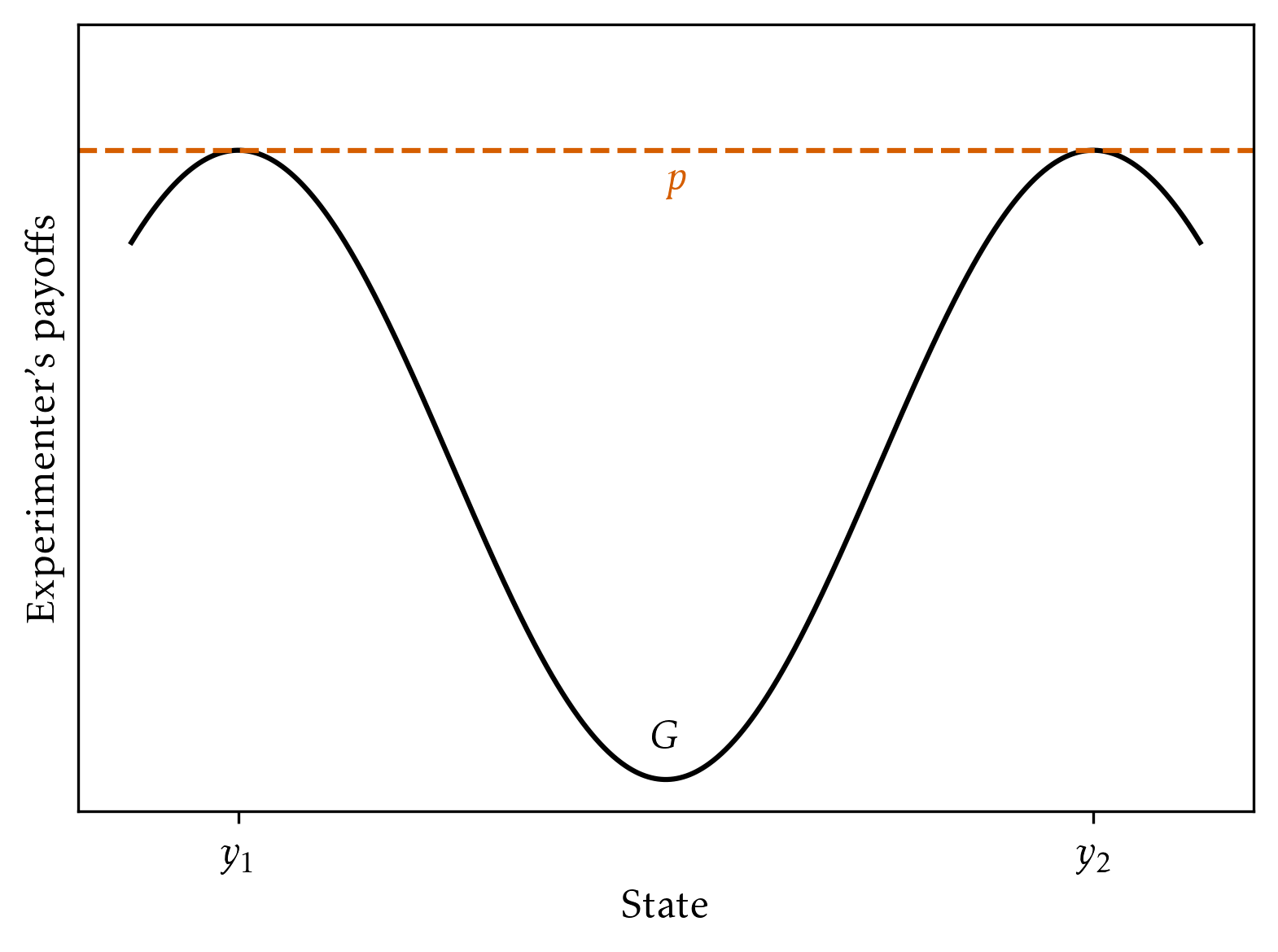
Suppose the experimenter’s payoff $G$ is $M$-shaped as in Figure˜6: concave on an interval of the lowest states, then convex, and finally concave on an interval of the highest states. In this example, $G$ has locally strict preferences. We now discuss incomplete full revelation, which also involves the prior $H$ of the state.

Figure˜6(a) depicts a situation in which the binary experiment $F^{\ast}$ that is supported on the peaks of the $M$ is a valid MPC of $H$. Then, $F^{\ast}$ is also the experimenter’s unique best reply under full delegation (apply Corollary 2 of Dworczak and Martini (2019) with the price function in Figure˜6(a)). The full delegation outcome $F^{\ast}$ does not admit incomplete full revelation since it does not fully reveal the state on any non-trivial interval. Let us argue why no profitable restriction exists. Lemma˜2 implies that an arbitrary incentive-compatible experiment $F$ must be supported between the two peaks, i.e. $\operatorname*{supp}F\subseteq[y_{1},y_{2}]$. Among all such experiments, the binary experiment $F^{\ast}$ with support $\{y_{1},y_{2}\}$ (and mean $\mu$) is the most informative. Thus, full delegation is optimal for the designer.

Conversely, suppose the prior $H$ is such that the full delegation outcome $F^{\ast}$ reveals states in an interval $[x_{1},x_{2}]$ in the valley between the peaks, and pools the remaining states to two points, $y_{1}$ and $y_{2}$, on the left and right slopes, as in Figure˜6(b). In particular, $F^{\ast}$ admits incomplete full revelation, and $F^{\ast}$ roughly looks like a lower censorship experiment and an upper censorship experiment patched together. Following our perturbation argument for upper censorship experiments from the $S$-shaped case, the designer can strictly improve on full delegation by pooling a small interval of states around each of $x_{1}$ and $x_{2}$.

(a) Full delegation is optimal.

(b) Full delegation is suboptimal.

Figure 6: Examples of $M$-shaped delegation of information provision.

General experimenter preferences.

The preceding examples suggest that profitable restrictions exist when the experimenter has locally strict preferences, and the full delegation outcome reveals some but not all states. We formalize these notions and the claim in Appendix˜B. Here, we give an informal description.

First, we formalize locally strict preferences as follows. There is a partition of the state space $[0,1]$ into finitely many intervals on each of which $G$ is either strictly convex or strictly concave, and if $G$ is tangential to a price function at specific points, then $G$ is also tangential to a (possibly distinct) price function at nearby distinct points. With price functions characterizing incentive-compatibility, the key implication is that relevant incentive-compatible experiments can be approximated by distinct incentive-compatible experiments. This condition is violated, for example, if the DM is uninformed—$G$ is a step function—since then the largest point in the support of any incentive-compatible experiment is at the step of $G$.

Second, we conceptualize incomplete full revelation under full delegation by considering the extreme points of $\operatorname*{MPC}(H)$. To that end, we first note that there exists an extreme point of $\operatorname*{MPC}(H)$ that is designer-preferred among the experimenter’s best replies under full delegation. We refer to such an extreme point as a DEF (designer-optimal extreme point under full delegation).

Let us recall the extreme-point characterization as bi-pooling experiments; see Kleiner et al. (2021); Arieli et al. (2023). For each extreme point $F$, there are countably many, disjoint bi-pooling intervals $[x_{1},x_{2}]$, such that $F$ pools $[x_{1},x_{2}]$ to at most two atoms and $I_{F}$ lies strictly below $I_{H}$ on the interior $(x_{1},x_{2})$. Outside the union of the bi-pooling intervals, $I_{F}$ coincides with $I_{H}$. We say a non-degenerate interval $[a,b]$ is fully revealing if $I_{F}$ coincides with $I_{H}$ on $[a,b]$. Note, an extreme point may not admit any fully revealing intervals, such as the binary experiment depicted in Figure˜6(a).

We say that an extreme point $F$ of $\operatorname*{MPC}(H)$ admits incomplete full revelation if $F$ fully reveals the state on non-degenerate intervals to the left and right of some bi-pooling interval, or only to one side of it if the bi-pooling interval admits a single atom and lies at the boundary of the state space. The experiment depicted in Figure˜6(a) does not admit incomplete full revelation since it admits no fully revealing intervals. The experiment depicted in Figure˜6(b) and all non-degenerate upper censorship experiments from the $S$-shaped case admit incomplete full revelation.

Our claim is thus that full delegation is suboptimal if the experimenter has locally strict preferences and there exists a DEF that admits incomplete full revelation. The formal details of the definitions and the proof are in Appendix˜B.

6.3 MIC Experiments as Extreme Points

We establish a link between extreme points of $\operatorname*{MPC}(H)$ and MIC experiments for general experimenter payoffs $G$. The literature has demonstrated how unrestricted persuasion problems are solved via extreme points of $\operatorname*{MPC}(H)$. The contribution of this section is to show that extreme points of $\operatorname*{MPC}(H)$ likewise solve the problem of designing restrictions subject to incentive constraints.

Let $G$ be upper semicontinuous with at most finitely many discontinuities at interior points $y_{1},\ldots,y_{k}\in(0,1)$, and Lipschitz continuous in each interval $(y_{i},y_{i+1})$, with $y_{0}=0$ and $y_{k+1}=1$; this is part (i) of the regularity condition of Dworczak and Martini (2019).

The definitions of incentive-compatibility and maximality are as in the baseline model, and MIC experiments are without loss (see Section˜A.2). Our price-theoretic characterization of incentive-compatibility (Lemma˜2) remains applicable given the regularity assumption on $G$. In contrast, our characterization of MIC experiments as double censorship makes explicit use of $S$-shapedness of $G$ and, hence, does not apply here.

At first sight, the extreme points of $\operatorname*{MPC}(H)$ and MIC experiments may seem unrelated. The extreme point characterization reflects the feasibility constraints of being a mean-preserving contraction of $H$; in particular, the characterization is independent of preferences. In contrast, MIC experiments are precisely characterized by the experimenter’s incentives to garble information. Nevertheless:

Theorem 3.

Every MIC experiment is an extreme point of $\operatorname*{MPC}(H)$.

Since Theorem˜3 shows that MIC experiments are extreme points of the entire set $\operatorname*{MPC}(H)$, the literature’s characterization of the extreme points as bi-pooling experiments applies under the novel MIC constraint.

Our proof leverages the characterization of extreme points as bi-pooling experiments. For a high-level intuition, note that any experiment $F\in\operatorname*{MPC}(H)$ is weakly increasing, and that the ICDF of $F$ lies weakly below the ICDF of the prior $H$. Roughly, the extreme point characterization states that at least one of these two constraints must bind locally. When the monotonicity constraint binds on an interval, $F$ assigns no mass to this interval; when the ICDF constraint binds, $F$ is maximally informative on this interval. Likewise, incentive-compatibility and maximality are characterized by two constraints on the respective experiment. Incentive-compatibility requires that $F$ assigns no mass to certain intervals (Lemma˜2); this is akin to the binding monotonicity constraint. Maximality requires that $F$ is maximally informative otherwise; this is akin to the binding informativeness constraint.

Moreover, leveraging the construction of Arieli et al. (2023) we can show that all MIC experiments are exposed. Thus, they arise as the unique persuasion solutions for a virtual sender; i.e., given MIC $F$ there exists a continuous virtual value

$$v_{F}\colon[0,1]\to\mathbb{R}\quad\mbox{such that}\quad F=\operatornamewithlimits{argmax}_{\tilde{F}\in\operatorname*{MPC}(H)}\intop\nolimits_{0}^{1}v_{F}(m)\mathop{}\!\mathrm{d}\tilde{F}(m).$$

Interestingly, in our context a virtual value can be chosen to capture the tension between the designer’s objective $u_{D}$ and the experimenter’s incentives. Starting from the designer’s strictly convex posterior-mean payoff $u_{D}$, define a convex “designer envelope” $p_{F}:[0,1]\to\mathbb R$ by letting $p_{F}(m)=u_{D}(m)$ for $m$ outside all bi-pooling intervals, and letting $p_{F}$ be affine on each bi-pooling interval. Next, let $p^{\ast}$ be any price function witnessing that $F$ is incentive-compatible for the experimenter in the sense of Lemma˜2. One can then directly check that, for any $\varepsilon>0$, a valid choice for the virtual sender payoff is

$$v_{F}(m)=p_{F}(m)-\varepsilon\mathopen{}\mathclose{{\left(p^{\ast}(m)-G(m)}}\right).$$

Note that the correction term $p^{\ast}-G$ is the experimenter’s incentive-compatibility constraint slackness. Therefore, $v_{F}$ captures the designer’s desire for information (via the convex $p_{F}$, built from $u_{D}$) but discounts the value of posterior means in proportion to the experimenter’s garbling incentives (via the slack $p^{\ast}-G$).

Theorem˜3 and our virtual value construction showcase how the literature’s extreme-point and linear-duality approaches can be combined to solve information design problems under incentive-compatibility and maximality constraints. In Appendix˜C, we show that incentive-compatible bi-pooling experiments are without loss more generally: each incentive-compatible experiment can be represented as a mixture of incentive-compatible bi-pooling experiments. This representation is useful when the designer’s preferences do not justify MIC experiments.

7 Conclusions

We analyze delegated information provision when the party producing information, the experimenter, has persuasion incentives and can always garble any admissible experiment before it reaches a decision maker. The designer cannot impose experiments upon the experimenter, but exerts control only by imposing a Blackwell-upper bound on informativeness.

The main conceptual contribution is to reduce optimal restriction design to the study of maximal incentive-compatible (MIC) experiments. An experiment is incentive compatible if it is self-enforcing: when the designer sets it as the upper bound, the experimenter optimally implements it rather than garbling. It is maximal if no strictly more informative experiment is also incentive compatible. Because the designer values information, we show that it is without loss to compare only MIC experiments.

In the baseline case of $S$-shaped experimenter preferences, MIC experiments are fully characterized as double censorship experiments. These reveal low states, pool an intermediate region to an interior atom, and pool high states to a top atom. Crucially, full delegation produces upper censorship (pooling all sufficiently high states), which is itself an extreme case of double censorship. Yet, we show that the designer always strictly prefers a nontrivial double-censorship restriction to full delegation.

The key takeaway is that profitable restrictions reallocate informativeness across states to discipline persuasion: sacrificing some precision in intermediate states relaxes the experimenter’s incentives to censor high states, yielding a strict gain for the designer.

Appendix A Proofs

A.1 Existence of an Optimal Restriction

Equip $\operatorname*{MPC}(H)$ with the $L^{1}$-norm, making it compact.

Lemma 5.

The set of IC experiments is a compact subset of $\operatorname*{MPC}(H)$. There exists an optimal IC experiment.

Existence can be shown by adapting Lemma 1 of Lipnowski et al. (2020), who consider settings with an abstract state. For the sake of completeness, we give a simple argument for our setting with posterior-mean payoffs. The proof does not use $S$-shapedness, but only upper semicontinuity of the designer’s and the experimenter’s payoffs.

Proof of Lemma˜5.

Existence of an optimal IC experiment follows from Berge’s Maximum Theorem and upper semicontinuity of the designer’s payoffs if we can show that the set of IC experiments is compact. Compactness follows if we can show that $\operatorname*{BR}$ is an upper hemicontinuous, nonempty- and compact-valued correspondence from $\operatorname*{MPC}(H)$ to itself. These properties of $\operatorname*{BR}$ follow from Lemma 17.30 of Aliprantis and Border (2006) and upper semicontinuity of the experimenter’s payoffs if we can show that $\operatorname*{MPC}$ is a continuous, compact-valued correspondence from $\operatorname*{MPC}(H)$ to itself. Compact-valuedness and upper hemicontinuity are straightforward.

As for lower hemicontinuity, let $(\bar{F}_{n})_{n\in\mathbb{N}}$ be a sequence in $\operatorname*{MPC}(H)$ converging to $\bar{F}\in\operatorname*{MPC}(H)$, and let $\Phi\in\operatorname*{MPC}(\bar{F})$. We have to find a subsequence of $({}_{n})_{n\in\mathbb{N}}$ converging to such that ${}_{n}\in\operatorname*{MPC}(\bar{F}_{n})$ for all $n$ in the subsequence. Note, $L^{1}$-convergence of $(\bar{F}_{n})_{n\in\mathbb{N}}$ to $\bar{F}$ implies pointwise convergence of $(I_{\bar{F}_{n}})_{n\in\mathbb{N}}$ to $I_{\bar{F}}$. For all $n$ and $m$, let $\tilde{J}_{n}(m)=\min\{I(m),I_{\bar{F}_{n}}(m)\}$. Since ICDFs are Lipschitz-continuous with constant $1$, the Arzelà–Ascoli Theorem delivers a uniformly convergent subsequence of $(\tilde{J}_{n})_{n}$. By possibly relabeling, let this be the entire sequence. The limit of the sequence $(\tilde{J}_{n})_{n}$ equals $I$ since $I_{\bar{F}_{n}}\to I_{\bar{F}}$ pointwise and since $I\leq I_{\bar{F}}$. Now, for all $n$, let $J_{n}$ be the lower convex hull of $\tilde{J}_{n}$. Let $\varepsilon_{n}=\|\tilde{J}_{n}-I\|_{\infty}$, so that $I-\varepsilon\leq\tilde{J}_{n}\leq I$. Since $I-\varepsilon_{n}$ is convex, and since $J_{n}$ is the lower convex hull of $\tilde{J}_{n}$, we have $I-\varepsilon_{n}\leq J_{n}\leq I$. In particular, $(J_{n})_{n}$ converges uniformly to $I$. Since, for all $n$, the function $J_{n}$ is convex and weakly increasing, it admits a weakly positive, weakly increasing derivative _n; i.e. $J_{n}=I_{{}_{n}}$. Using that $J_{n}\leq I$ and $J_{n}(1)=I(1)$, one may verify ${}_{n}(m)\leq 1$ for all $m\in[0,1]$. In particular, _n is in $\operatorname*{MPC}(H)$. In fact, since $I_{{}_{n}}\leq J_{n}\leq\tilde{J}_{n}\leq I_{\bar{F}_{n}}$, we have ${}_{n}\in\operatorname*{MPC}(\bar{F}_{n})$. Finally, by possibly passing to a further subsequence and invoking Helly’s Selection Theorem, let $({}_{n})_{n}$ converge pointwise to, say, $\tilde{\Phi}$. By Dominated Convergence, the sequence $(I_{{}_{n}})_{n}$ (i.e. the sequence $(J_{n})_{n}$) converges pointwise to $I_{\tilde{\Phi}}$. We have already argued that the sequence $(I_{{}_{n}})_{n}$ (i.e. the sequence $(J_{n})_{n}$) converges pointwise to $I$. Thus, $I=I_{\tilde{\Phi}}$, implying $\Phi=\tilde{\Phi}$ almost everywhere. Thus, $({}_{n})_{n}$ converges pointwise a.e. to and, hence, also with respect to the $L^{1}$-norm. ∎

A.2 Proof of LABEL:{lemma:MIC_wlog}

Consider the auxiliary problem of maximizing $\intop\nolimits\exp(m)\mathop{}\!\mathrm{d}\tilde{F}(m)$ across incentive-compatible experiments $\tilde{F}$ in $\operatorname*{MPC}(H)\cap\operatorname*{MPS}(F)$. Incentive-compatible experiments form a compact subset of $\operatorname*{MPC}(H)$ when $G$ is upper semicontinuous (Lemma˜5). In particular, the constraint set of the auxiliary problem is also compact. Hence, a solution exists. By construction, the solution is incentive-compatible and a mean-preserving spread of $F$. The solution is maximal since $\exp$ is strictly convex, and since any experiment that is a mean-preserving spread of $\tilde{F}$ is also a mean-preserving spread of $F$. ∎

Remark.

Our proof of Lemma˜1 did not use $S$-shapedness of $G$, but only upper semicontinuity of $G$. Here, we sketch an alternative constructive proof that relies on $S$-shapedness and some upcoming lemmata for that case. Given an incentive-compatible experiment $F$, following the proof of the upcoming Lemma˜6, one can find a double censorship experiment $\hat{F}$ that is IC and an MPS of $F$. (Possibly, $\hat{F}$ is unrestricted persuasion, which is also a form of double censorship.) Moreover, the atoms $(\hat{x},\hat{y})$ of $\hat{F}$ satisfy $(\hat{x},\hat{y})\in P$ and $[x^{\ast},y^{\ast}]\subseteq[\hat{x},\hat{y}]$. Now, the upcoming Lemma˜7 implies that $\hat{F}$ is maximal.

A.3 Proof of Lemma˜3

To prove one part of the equivalence, let $F\in\operatorname*{MPC}(H)$ be IC and non-degenerate. Let $p$ be as in Lemma˜2. If $\max\operatorname*{supp}F\leq r_{0}$, then, definitionally, $F$ assigns no mass to $(r_{0},1]$. The proof is complete for $x=y=r_{0}$, since $(r_{0},r_{0})\in P$. In what follows, let $\max\operatorname*{supp}F>r_{0}$. Let $y=\max\operatorname*{supp}F$, so that $p(y)=G(y)$. We find a point $x<r_{0}$ such that $(x,y)\in P$ and such that $F$ assigns no mass to $(x,y)\cup(y,1]$.

Recall that $G$ is strictly concave on $[r_{0},1]$. Since $p$ is convex and $p\geq G$ holds, there exists at most one point in $[r_{0},1]$ at which $p$ and $G$ coincide. Since $y>r_{0}$, this point is $y$. Thus, $\operatorname*{supp}F\cap(r_{0},1]$ contains only $y$. Since $F$ is non-degenerate, the intersection $\operatorname*{supp}F\cap[0,r_{0}]$ is non-empty. Let $\tilde{x}=\max(\operatorname*{supp}F\cap[0,r_{0}])$. In particular, $p(\tilde{x})=G(\tilde{x})$ and $\tilde{x}\leq r_{0}$.

Now, recall $p\geq G$ and $p(y)=G(y)$, so that $p-G$ is minimized at $y$. Since $p$ is convex while $G$ is concave on a neighborhood of $y$, the subdifferential of $p$ at $y$ contains $g(y)$. Since also $p(\tilde{x})=G(\tilde{x})$, we infer $G(\tilde{x})+g(y)(y-\tilde{x})=p(\tilde{x})+g(y)(y-\tilde{x})\geq p(y)=G(y)$, where the last inequality follows by definition of the subdifferential. We also know $G(r_{0})+g(y)(y-r_{0})<G(y)$ since $G$ is strictly concave on $[r_{0},1]$. Thus, $\tilde{x}<r_{0}$ and, by continuity, there exists $x\in[\tilde{x},r_{0})$ such that $G(x)+g(y)(y-x)=G(y)$. That is, $(x,y)\in P$. Since $\tilde{x}=\max(\operatorname*{supp}F\cap[0,r_{0}])\leq x$ and $\operatorname*{supp}F\cap(r_{0},1]=\{y\}$, we conclude that $F$ assigns no mass to $(x,y)\cup(y,1]$.

To prove the other part of the equivalence, let $(x,y)\in P$ and $F\in\operatorname*{MPC}(H)$ be such that $F$ is non-degenerate and assigns no mass to $(x,y)\cup(y,1]$. In view of Lemma˜2, we can show that $F$ is IC by finding a convex function $p$ such that $p\geq G$ and such that $p=G$ holds on $\operatorname*{supp}F$. Let $p(m)=G(m)$ for all $m\in[0,x]$, and $p(m)=G(x)+g(y)(m-x)$ for all $m\in[x,1]$. Note $p(y)=G(y)$ since $(x,y)\in P$. Clearly, $p=G$ holds on $\operatorname*{supp}F$ since $F$ assigns no mass to $(x,y)\cup(y,1]$. We next argue $p\geq G$. On $[r_{0},1]$, the function $G$ is concave whereas $p$ is affine. Since $p(y)=G(y)$, it holds $p\geq G$ on $[r_{0},1]$. On $[x,r_{0}]$ (recall $x\leq r_{0}$ from the definition of $P$), the function $G$ is convex whereas $p$ is affine. Since $p(x)=G(x)$ but $p(r_{0})\geq G(r_{0})$ (as already argued), we find $p\geq G$ on $[x,r_{0}]$. It remains to argue that $p$ is convex. Clearly, $p$ is convex on $[0,x]$. Since $p$ is affine on $[x,1]$ with slope $g(y)$, global convexity follows if we can show $g(y)\geq g(x)$. This inequality, in turn, holds since $p\geq G$ and $p(x)=G(x)$ both hold. ∎

A.4 Proof of LABEL:{lemma:p_order}

For all $(x,y)$ such that $0\leq x\leq r_{0}\leq y\leq 1$, let $\rho(x,y)=G(x)+g(y)(y-x)-G(y)$. By definition of $P$, if $(x,y)\in P$, then $\rho(x,y)=0$. We show that $\rho$ is strictly single-crossing from above in each argument (holding the other fixed). Therefore, if $(x,y)$ and $(x^{\prime},y^{\prime})$ are both in $P$, then $[x,y]$ and $[x^{\prime},y^{\prime}]$ are ordered by set inclusion.

For all $(x,y)$ such that $0\leq x\leq r_{0}\leq y\leq 1$, it holds $\partial\rho(x,y)/\partial y=g^{\prime}(y)\leq 0$, where the inequality holds since $r_{0}\leq y$ and since $G$ is concave on $[r_{0},1]$; further, $g^{\prime}(y)<0$ if $r_{0}<y$. Thus, $\tilde{y}\mapsto\rho(x,\tilde{y})$ (defined on $[r_{0},1]$) is strictly single-crossing from above.

For all $(x,y)$ such that $0\leq x\leq r_{0}\leq y\leq 1$, it holds $\partial\rho(x,y)/\partial x=g(x)-g(y)$. We claim $g(x)<g(y)$ if $\rho(x,y)=0$ and $x<y$, which suffices to establish that $\tilde{x}\mapsto\rho(\tilde{x},y)$ (defined on $[0,r_{0}]$) is strictly single-crossing from above. Towards a contradiction, let $g(x)\geq g(y)$. Since $g$ is strictly quasiconcave, all $r\in(x,y)$ satisfy $g(r)>g(y)$, implying $G(y)-G(x)>g(y)(y-x)$, which contradicts $\rho(x,y)=0$. ∎

A.5 Proof of LABEL:{thm:MIC_characterization}

For reference, we record the ICDF of a double censorship experiment $F$ with thresholds $(s,t)$ and atoms $(x,y)$:

$$\forall m\in[0,1],\quad I_{F}(m)=\begin{cases}I_{H}(m)\quad&\mbox{if }m\in[0,s],\\ I_{H}(s)+H(s)(m-s)\quad&\mbox{if }m\in(s,x],\\ I_{H}(t)+H(t)(m-t)\quad&\mbox{if }m\in(x,y],\\ m-\mu,\quad&\mbox{if }m\in(y,1].\end{cases}$$

In words, $I_{F}$ coincides with $I_{H}$ on $[0,s]$, and is then piecewise affine, being tangent to $I_{H}$ at ($s$ and) $t$, and coincides with $I_{\delta_{\mu}}$ on $[y,1]$.

We separately prove the two parts of the equivalence claimed by Theorem˜1.

Lemma 6.

If $F$ is an MIC experiment, then $F$ is non-degenerate double censorship for a pair of thresholds $(s,t)$ and atoms $(x,y)$ such that $(x,y)\in P$ and $s\leq x^{\ast}\leq t$ and $0<x<y<1$.

Proof of Lemma˜6.

The experiment must be non-degenerate since, otherwise, it is a strict MPC of $F^{\ast}$, contradicting maximality. Hence, we can appeal to Lemma˜3 to find $(x,y)\in P$ such that $F$ assigns no mass to $(x,y)\cup(y,1]$.

We next claim $[x^{\ast},y^{\ast}]\subseteq[x,y]$. By Lemma˜4, it holds $[x^{\ast},y^{\ast}]\subseteq[x,y]$ or $[x,y]\subseteq[x^{\ast},y^{\ast}]$. In the first case, we are done, so let $[x,y]\leq[x^{\ast},y^{\ast}]$. We show that $F$ is an MPC of $F^{\ast}$; by maximality, it follows $F=F^{\ast}$ and, hence, $[x,y]=[x^{\ast},y^{\ast}]$. To show $F$ is an MPC of $F^{\ast}$, we show $I_{F}\leq I_{F^{\ast}}$ on $[0,1]$. Clearly, $I_{F}\leq I_{H}=I_{F^{\ast}}$ on $[0,x^{\ast}]$. Next, we know $I_{F}$ coincides with $I_{\delta_{\mu}}$ on $[y,1]$, whereas $I_{F^{\ast}}$ coincides with $I_{\delta_{\mu}}$ on $[y^{\ast},1]$. Since $y\leq y^{\ast}$, we infer $I_{F}=I_{F^{\ast}}$ on $[y^{\ast},1]$. In summary, $I_{F}\leq I_{F^{\ast}}$ on $[0,x^{\ast}]\cup[y^{\ast},1]$. Finally, since $F^{\ast}$ assigns no mass to $(x^{\ast},y^{\ast})$, the integrated CDF $I_{F^{\ast}}$ is affine on $[x^{\ast},y^{\ast}]$. Since $I_{F}$ is convex and lies below $I_{F^{\ast}}$ at the endpoints of this interval (as already argued), it follows $I_{F}\leq I_{F^{\ast}}$ also on $[x^{\ast},y^{\ast}]$. Thus, $I_{F}\leq I_{F^{\ast}}$ on $[0,1]$.

We next show that $F$ is double censorship. The idea is to construct an MPS $\tilde{F}$ of $F$ that is double censorship and IC. Since $F$ is MIC, it will follow $\tilde{F}=F$.

Our candidate double censorship will use $(x,y)$ as atoms. We thus show next that $(x,y)$ can arise as atoms for some choice of thresholds $(s,t)$. First, since $y^{\ast}=\mathbb{E}_{H}[\bm{\omega}\mid\bm{\omega}\in[x^{\ast},1]]$ and $y^{\ast}\leq y\leq 1$, there exists $t\in[x^{\ast},y]$ such that $y=\mathbb{E}_{H}[\bm{\omega}\mid\bm{\omega}\in[t,1]]$. Note, $t\in[x,y]$ since $x\leq x^{\ast}$. Second, we argue there exists $s\in[0,x^{\ast}]$ such that $x=\mathbb{E}_{H}[\bm{\omega}\mid\bm{\omega}\in[s,t]]$. By construction, it holds $y=\mathbb{E}_{H}[\bm{\omega}\mid\bm{\omega}\in[t,1]]$, which rearranges to $I_{F}(y)=I_{H}(t)+H(t)(y-t)$. The affine map $m\mapsto I_{H}(t)+H(t)(m-t)$ lies above $I_{F}$ at $m=t$ (since $I_{F}(t)\leq I_{H}(t)$) and coincides with $I_{F}$ at $m=y$ (by construction of $t$). Since also $I_{F}$ is affine on $[x,y]$ (since $F$ assigns no mass to $(x,y)$), and since two affine maps on $\mathbb{R}$ either coincide or intersect at most once, we conclude $I_{F}(x)\leq I_{H}(t)+H(t)(x-t)$. Let $\xi=I_{H}(t)+H(t)(x-t)$. In particular, $\xi\geq I_{F}(x)\geq 0$. We also have $\xi\leq I_{H}(x)$ since the affine map $\tilde{t}\mapsto I_{H}(t)+H(t)(\tilde{t}-t)$ is tangent to the convex map $I_{H}$ at $t$. Finally, find $s\in[0,x]$ such that $I_{H}(s)+H(s)(x-t)=\xi$; this is possible since $\xi\in[0,I_{H}(x)]$. Thus, $I_{H}(s)+H(s)(x-t)=I_{H}(t)+H(t)(x-t)$, which rearranges to $x=\mathbb{E}_{H}[\bm{\omega}\mid\bm{\omega}\in[s,t]]$.

Now let be double upper censorship with thresholds $(s,t)$ and atoms $(x,y)$. Notice that is IC; indeed, assigns no mass to the set $(x,y)\cup(y,1]$ (by definition of upper censorship), and it holds $(x,y)\in P$ (as argued at the very beginning of the proof); now invoke Lemma˜3.

We now argue is an MPS of $F$. Clearly, $I=I_{H}\geq I_{F}$ on $[0,s]$, and $I=I_{\delta_{\mu}}=I_{F}$ on $[y,1]$. For $\tilde{t}\in[x,y]$ it holds $I(\tilde{t})=I_{H}(t)+H(t)(\tilde{t}-t)\geq I_{F}(t)$, where the inequality follows from the argument that constructed $s$. Finally, it holds $I\geq I_{F}$ on $[s,x]$ since $I$ is affine on this interval, $I_{F}$ is convex, and since $I\geq I_{F}$ holds at the endpoints of this interval (as already argued). Thus, is an MPS of $F$.

It remains to show $s\leq x^{\ast}\leq t$ and $0<x<y<1$. The inequalities $s\leq x^{\ast}\leq t$ follow from $[x^{\ast},y^{\ast}]\subseteq[x,y]$ and the expressions for $x$, $y$, and $y^{\ast}$ as conditional expectations. From $[x^{\ast},y^{\ast}]\subseteq[x,y]$ and $x^{\ast}<r_{0}<y^{\ast}$, we also obtain $x<y$.

Next, towards a contradiction, let $y=1$. Then also $t=1$ (since $y=\mathbb{E}_{H}[\bm{\omega}\mid\bm{\omega}\in[t,1]]$), meaning $x$ is the largest point in the support of $F$. From $y=1>y^{\ast}$ we also get $x<x^{\ast}$ (Lemma˜4). It now follows easily that $F$ is a proper MPC of $F^{\ast}$; indeed, $I_{F}=I_{\delta_{\mu}}\leq I_{F}^{\ast}$ on $[x,1]$; this inequality is strict on $(x,x^{\ast})$ since $I_{F}$ is affine on this interval whereas $I_{F^{\ast}}$ is strictly convex (it coincides with $I_{H}$); finally, $I_{F}\leq I_{F^{\ast}}\leq I_{H}$ on $[0,x]$. Thus, $F$ is a proper MPC of $F^{\ast}$, contradicting maximality of $F$. Thus, $y<1$.

Finally, towards a contradiction, let $x=0$. This requires $s=t=0$ since $x=\mathbb{E}_{H}[\bm{\omega}\mid\bm{\omega}\in[s,t]]$. It follows that $F$ is degenerate on $y$; contradiction. ∎

Lemma 7.

If $F$ is double censorship for a pair of thresholds $(s,t)$ and atoms $(x,y)$ such that $(x,y)\in P$ and $s\leq x^{\ast}\leq t$ and $0<x<y<1$, then $F$ is MIC.

Proof of Lemma˜7.

Lemma˜3 implies that $F$ is IC. To prove that $F$ is maximal, let be IC and such that $I_{F}\leq I$. We show $I_{F}=I$. Let $\hat{y}=\max\operatorname*{supp}\Phi$.

First, we show $\hat{y}<y$ cannot hold. Indeed, the function $I$ coincides with $m\mapsto m-\mu$ on $[\hat{y},1]$. Meanwhile, $I_{F}$ coincides with $m\mapsto m-\mu$ on $[y,1]$ but has slope of at most $H(t)$ on $[0,y)$. Since $t\leq y<1$, we have $H(t)<1$. Thus, if $\hat{y}<y$, then $I_{F}$ lies strictly above $I$ on $(\hat{y},y)$, contradicting $I_{F}\leq I$.

Thus, let $\hat{y}\geq y$. Since $\hat{y}=\max\operatorname*{supp}\Phi$ and $y>r_{0}$, the IC characterization (Lemma˜3) implies there exists $\hat{x}\leq r_{0}$ such that $(\hat{x},\hat{y})\in P$ and such that assigns no mass to $(\hat{x},\hat{y})\cup(\hat{y},1]$. Since $\hat{y}\geq y$, Lemma˜4 implies $\hat{x}\leq x$.

Since assigns no mass to $(\hat{x},\hat{y})$, and since $[x,y]\subseteq[\hat{x},\hat{y}]$ and $t\in[x,y]$, we conclude that $I$ is affine on $[\hat{x},\hat{y}]$ and this interval contains $t$. Now, since $F$ is double censorship, $I_{F}$ is tangential to $I_{H}$ at $t$. Thus, also $I(t)=I_{H}(t)$ since $I_{F}\leq I\leq I_{H}$. Thus, is affine with slope $H(t)$ on $[\hat{x},\hat{y}]$. Since $F$ is affine $[x,y]$ (a subset of $[\hat{x},\hat{y}]$) and tangential to $I_{H}$ at $t$, it follows that and $F$ coincide on $[x,y]$. From here and the inclusion $[x,y]\subseteq[\hat{x},\hat{y}]$, it readily follows $I_{F}=I=I_{\delta_{\mu}}$ on $[y,1]$.

We also know that $I_{F}$ and $I$ coincide on $[0,s]$ since on this interval $I_{F}=I_{H}\geq I\geq I_{F}$. It now follows $I_{F}=I$ on $[s,x]$ since $I_{F}$ is affine on this interval, $I$ is convex, and since the two coincide at the endpoints (as already argued). Thus, $I_{F}=I$. ∎

Lemmata˜6 and 7 together prove Theorem˜1. ∎

A.6 Proof of LABEL:{cor:MIC_total_order}

Let $(s,t,x,y)$ and $(s^{\prime},t^{\prime},x^{\prime},y^{\prime})$ be the parameters of two MIC experiments such that $y^{\prime}<y$. Since $(x,y)\in P$ and $(x^{\prime},y^{\prime})\in P$ (Theorem˜1), Lemma˜4 implies $x\leq x^{\prime}$; the proof of this lemma delivers $x<x^{\prime}$. Using the expressions for $x$, $x^{\prime}$, $y$, and $y^{\prime}$ as conditional expectations, it also follows $[s^{\prime},t^{\prime}]\subsetneq[s,t]$ and $[t,1]\subsetneq[t^{\prime},1]$ and $x<x^{\prime}$. ∎

A.7 Proof of LABEL:{cor:double_censorship_implementation}

We apply Corollary 1 of Dworczak and Martini (2019) (cited in the proof of Lemma˜2). Let $p$ be the function that coincides with $G$ on $[0,x]$, and coincides with the affine map $m\mapsto G(x)+g(y)(m-x)$ for $m\in(x,1]$. Then, $p$ is convex, weakly above $G$, and coincides with $G$ on $[0,x]$ and $y$; see the proof of Lemma˜3 for this argument. Moreover, $\operatorname*{supp}F\subseteq\{m\in[0,1]\colon p(m)=G(m)\}$ since $F$ is double censorship with parameters $(s,t,x,y)$. Finally, it holds $\intop\nolimits p\mathop{}\!\mathrm{d}F=\intop\nolimits p\mathop{}\!\mathrm{d}\bar{F}$. Indeed, we have $F=\bar{F}=H$ on $[0,s]$. Conditioned on the interval $[s,t]$, both $F$ and $\bar{F}$ are degenerate on $x$. Finally, on the interval $[t,1]$, the function $p$ is affine and $F$ is obtained by pooling $\bar{F}$. Thus, $\intop\nolimits p\mathop{}\!\mathrm{d}F=\intop\nolimits p\mathop{}\!\mathrm{d}\bar{F}$. By Corollary 1 of Dworczak and Martini (2019), the experiment $F$ is a best reply to $\bar{F}$. ∎

A.8 Proof of LABEL:{thm:profitable_restriction}

The idea of the proof is to consider MIC double censorship, as parametrized by $(s,t,x,y)$, such that $y$ is close to the full delegation atom $y^{\ast}$; in this case, also $s$, $t$, and $x$ are all close to $x^{\ast}$. We evaluate the designer’s first-order gain from this perturbation and show that it is strictly positive.

Lemma˜3 implies that a tuple $(s,t,x,y)$ with $0\leq s\leq x\leq t\leq y<1$ and $x\leq r_{0}\leq y$ represents an IC double censorship if

$$G(x)+g(y)(y-x)-G(y) =0,$$ (6a)

$$\intop\nolimits_{[t,1]}(\omega-y)\mathop{}\!\mathrm{d}H(\omega) =0,$$ (6b)

$$\intop\nolimits_{[s,t]}(\omega-x)\mathop{}\!\mathrm{d}H(\omega) =0,$$ (6c)

all hold. (In fact, in this case the experiment is MIC.) We know that one such tuple is $(s,t,x,y)=(x^{\ast},x^{\ast},x^{\ast},y^{\ast})$, where $x^{\ast}$ is the threshold and $y^{\ast}$ is the atom under full delegation. We next argue that for all $y$ sufficiently close to $y^{\ast}$ there exist $(s,t,x)$ satisfying the above.

Since $G$ is strictly concave on a neighborhood of $y^{\ast}$ but strictly convex on a neighborhood of $x^{\ast}$, for all $y>y^{\ast}$ sufficiently close to $y^{\ast}$ there exists $\hat{x}(y)<x^{\ast}$ such that $G(\hat{x}(y))+g(y)(y-\hat{x}(y))=G(\hat{x}(y))$, i.e. (6a) holds. Moreover, $\hat{x}(y)\to x^{\ast}$ as $y\to y^{\ast}$. Next, using $y^{\ast}<1$, it is easy to see (using, e.g., the Intermediate Value Theorem) that for all $y$ sufficiently close to $y^{\ast}$ there exists $\hat{t}(y)\in[0,y)$ solving (6b). Using the Inverse Function Theorem, on a neighborhood of $y^{\ast}$ the function $\hat{t}$ has the derivative

$$\frac{\partial\hat{t}(y)}{\partial y}=\frac{1-H(\hat{t}(y))}{(y-\hat{t}(y))h(\hat{t}(y))}>0.$$

For later reference, for $y>y^{\ast}$, equation (6b) requires $\hat{t}(y)>x^{\ast}$. Finally, using also $0<x^{\ast}<y^{\ast}<1$, it is easy to see that for all $y$ sufficiently close to $y^{\ast}$ there exists $\hat{s}(y)\in(0,\hat{x}(y))$ such that $(\hat{s}(y),\hat{t}(y),\hat{x}(y),y)$ satisfies (6c).

Thus, for some $\varepsilon>0$ and all $y\in(y^{\ast},y^{\ast}+\varepsilon]$, the tuple $(\hat{s}(y),\hat{t}(y),\hat{x}(y),y)$ defines an MIC double censorship experiment. We show that for $y$ sufficiently close to $y^{\ast}$ the designer is strictly better off than under unrestricted persuasion. Note, for $y\searrow y^{\ast}$, we have $(\hat{s}(y),\hat{t}(y),\hat{x}(y))\to(x^{\ast},x^{\ast},x^{\ast})$ since, following the above arguments, there is a unique solution for eqs.˜6a, 6b and 6c that involves $y^{\ast}$, and $(x^{\ast},x^{\ast},x^{\ast},y^{\ast})$ is a solution.

The designer’s utility from $(\hat{s}(y),\hat{t}(y),\hat{x}(y),y)$, denoted $U_{D}(y)$, is given by

$$U_{D}(y)=\intop\nolimits_{[0,\hat{s}(y)]}u_{D}(\omega)\mathop{}\!\mathrm{d}H(\omega)+u_{D}(\hat{x}(y))(H(\hat{t}(y))-H(\hat{s}(y)))+u_{D}(y)(1-H(\hat{t}(y))).$$

The expected utility from $(x^{\ast},x^{\ast},x^{\ast},y^{\ast})$ is given by

$$U_{D}(y^{\ast})=\intop\nolimits_{[0,x^{\ast}]}u_{D}(\omega)\mathop{}\!\mathrm{d}H(\omega)+u_{D}(y^{\ast})(1-H(x^{\ast})),$$

which also obtains as the limit as $y\to y^{\ast}$ from above. Thus,

$$U_{D}(y)-U_{D}(y^{\ast})$$

$$= (u_{D}(y)-u_{D}(y^{\ast}))(1-H(x^{\ast}))+(u_{D}(y)-u_{D}(\hat{x}(y)))(H(x^{\ast})-H(\hat{t}(y)))$$ (7)

$$+\intop\nolimits_{[\hat{s}(y),x^{\ast}]}(u_{D}(\hat{x}(y))-u_{D}(\omega))\mathop{}\!\mathrm{d}H(\omega).$$ (8)

Dividing by $y-y^{\ast}$ and taking $y\to y^{\ast}$, the sum of the two terms in (7) converges to

$$u_{D}^{\prime}(y^{\ast})(1-H(x^{\ast}))-(u_{D}(y^{\ast})-u_{D}(x^{\ast}))h(x^{\ast})\mathopen{}\mathclose{{\left.\frac{\partial\hat{t}(y)}{\partial y}}}\right|_{y=y^{\ast}}$$

$$= \mathopen{}\mathclose{{\left(u_{D}^{\prime}(y^{\ast})-\frac{u_{D}(y^{\ast})-u_{D}(x^{\ast})}{y^{\ast}-x^{\ast}}}}\right)(1-H(x^{\ast}))>0,$$

where the strict inequality follows from strict convexity of $u_{D}$ and since $y^{\ast}>x^{\ast}$ holds. Thus, to show $U_{D}(y)>U_{D}(y^{\ast})$ for $y$ sufficiently close to $y^{\ast}$, it suffices to show that the integral in (8) admits a vanishing lower bound when normalized by $y-y^{\ast}$. Find $L>0$ such that $|u_{D}^{\prime}|\leq L$. Using this bound and the choice of $\hat{s}(y)$ in (6c), we have

$$\frac{1}{y-y^{\ast}}\intop\nolimits_{[\hat{s}(y),x^{\ast}]}(u_{D}(\hat{x}(y))-u_{D}(\omega))\mathop{}\!\mathrm{d}H(\omega)\geq \frac{-L}{y-y^{\ast}}\mathopen{}\mathclose{{\left|\intop\nolimits_{[\hat{s}(y),x^{\ast}]}(\hat{x}(y))-\omega)\mathop{}\!\mathrm{d}H(\omega)}}\right|$$

$$= \frac{-L}{y-y^{\ast}}\mathopen{}\mathclose{{\left|\intop\nolimits_{[x^{\ast},\hat{t}(y)]}(\hat{x}(y))-\omega)\mathop{}\!\mathrm{d}H(\omega)}}\right|$$

$$\geq \frac{-L}{y-y^{\ast}}\mathopen{}\mathclose{{\left|(\hat{x}(y)-x^{\ast})\mathopen{}\mathclose{{\left(H(\hat{t}(y))-H(x^{\ast})}}\right)}}\right|.$$

The lower bound vanishes since $\hat{t}(y)$ is differentiable at $y=y^{\ast}$ and $\hat{t}(y^{\ast})=x^{\ast}$, and since $\hat{x}(y)\to x^{\ast}$ as $y\to y^{\ast}$. ∎

A.9 Proof of LABEL:{thm:general_extreme_points}

Let $F$ be MIC. In view of Kleiner et al. (2021, Theorem 2), to show that $F$ is an extreme point of $\operatorname*{MPC}(H)$, we have to show that, for every open subinterval $(a,b)$ on which the ICDF of $F$ lies strictly below the ICDF of $H$, the support of $F$ has at most two points in $(a,b)$. To leverage that $F$ is maximal, we consider perturbations on such subintervals. We shall leverage the IC characterization, Lemma˜2, to argue that the perturbations are IC.

For later reference, also by Lemma˜2, there exists a continuous, convex function $p\colon[0,1]\to\mathbb{R}$ such that $p\geq G$ and $\operatorname*{supp}F\subseteq\{m\in[0,1]\colon p(m)=G(m)\}$.

Let $[a,b]$ be a subinterval of $[0,1]$ such that $I_{F}(m)<I_{H}(m)$ for all $m\in(a,b)$.

Let $m\in(\operatorname*{supp}F)\cap(a,b)$. We claim that there is a neighborhood $O$ of $m$ such that $(\operatorname*{supp}F)\cap O=\{m\}$. Towards a contradiction, suppose not. Then, there is a sequence $(m_{n})_{n\in\mathbb{N}}$ in $((\operatorname*{supp}F)\setminus\{m\})\cap(a,b)$ converging to $m$. By possibly passing to a subsequence, let the sequence be strictly monotone. Assume the sequence is strictly increasing, the case where it is strictly decreasing being similar. Find $n$ sufficiently large such that the line segment between $(m_{n},I_{F}(m_{n}))$ and $(m,I_{F}(m))$ does not intersect $I_{H}$ on the interval $[m_{n},m]$; such $n$ exits since $I_{F}$ lies strictly below $I_{H}$ on $(a,b)$ and since ICDFs are $1$-Lipschitz. Consider the function that coincides with $I_{F}$ below $m_{n}$ and above $m$, and that coincides with the chosen line segment on $[m_{n},m]$. This function is weakly increasing and convex, coincides with $I_{H}$ at $0$ and $1$, and lies below $I_{H}$. Thus, its derivative $\tilde{F}$ is an experiment. Since $m_{n}$ and $m$ are in the support of $F$, and since $I_{\tilde{F}}$ and $I_{F}$ coincide outside $[m_{n},m]$, it holds $\operatorname*{supp}\tilde{F}\subseteq\operatorname*{supp}F\subseteq\{m^{\prime}\in[0,1]\colon p(m^{\prime})=G(m^{\prime})\}$. In particular, Lemma˜2 implies that $\tilde{F}$ is IC. Finally, $\tilde{F}$ is an MPS of $F$ since $I_{F}$ is convex on $[m_{n},m]$ while $I_{\tilde{F}}$ is affine on this interval and coincides with $I_{F}$ at $m_{n}$ and $m$. Since $F$ is maximal, we infer $F=\tilde{F}$. In particular, $I_{F}$ is affine on $[m_{n},m]$, meaning $F$ assigns no mass to the open interval $(m_{n},m)$. However, by strict monotonicity, $m_{n+1}\in(m_{n},m)$, contradicting $m_{n+1}\in\operatorname*{supp}F$.

We now claim that for all closed subintervals $[c,d]$ of $(a,b)$ the intersection $(\operatorname*{supp}F)\cap[c,d]$ is finite. Indeed, for all $m\in(\operatorname*{supp}F)\cap[c,d]$, let $O_{m}$ be as in the previous paragraph, i.e. $(\operatorname*{supp}F)\cap O_{m}=\{m\}$. This yields an open cover of the compact set $(\operatorname*{supp}F)\cap[c,d]$. Now find a finite subcover to conclude that $(\operatorname*{supp}F)\cap[c,d]$ is finite.

Let $[c,d]\subseteq(a,b)$ be arbitrary. We claim $(\operatorname*{supp}F)\cap[c,d]$ contains at most two points. Towards a contradiction, suppose not. Since $(\operatorname*{supp}F)\cap[c,d]$ is finite, there exist three consecutive points $x,y,z$ in $(\operatorname*{supp}F)\cap[c,d]$; by “consecutive” we mean that there is no other point in $\operatorname*{supp}F$ between $x$ and $y$, nor between $y$ and $z$. In particular, $I_{F}$ is affine between $x$ and $y$; call the slope $\alpha$. Also, $I_{F}$ is affine between $y$ and $z$; call the slope $\beta$. Since $y$ is in the support of $F$, it holds $\alpha<\beta$. Consider the function $\tilde{J}$ obtained from $I_{F}$ by slightly raising $\alpha$ by $\varepsilon_{\alpha}>0$ while decreasing $\beta$ by $\varepsilon_{\beta}>0$, holding fixed $I_{F}$ at $x$ and at $z$. (Thus, $I_{F}$ is shifted up at $y$.) Finally, let $\tilde{J}$ coincide with $I_{F}$ outside $[x,z]$. For $\varepsilon_{\alpha}$ and $\varepsilon_{\beta}$ sufficiently small, the function $\tilde{J}$ is convex since $\alpha<\beta$. Moreover, since $I_{F}$ lies strictly below $I_{H}$ on $(a,b)$, and since $I_{F}$ is affine on each of $[x,y]$ and $[y,z]$, for $\varepsilon_{\alpha}$ and $\varepsilon_{\beta}$ sufficiently small also $\tilde{J}$ lies below $I_{H}$ on $[x,y]$ (and thus on all of $[0,1]$). Thus, the derivative of $\tilde{J}$, call it $\tilde{F}$, is an experiment. By construction $\tilde{F}$ is a proper MPS of $F$. Finally, since $\operatorname*{supp}\tilde{F}\subseteq\operatorname*{supp}F\subseteq\{m\in[0,1]\colon p(m)=G(m)\}$, Lemma˜2 implies that $\tilde{F}$ is IC; contradiction to maximality of $F$.

Since in the previous paragraph $[c,d]\subseteq(a,b)$ was arbitrary, the intersection $(\operatorname*{supp}F)\cap(a,b)$ contains at most two points. Since $[a,b]$ was an arbitrary interval such that $I_{F}<I_{H}$ on $(a,b)$, Theorem 2 of Kleiner et al. (2021) implies that $F$ is an extreme point of $\operatorname*{MPC}(H)$. ∎

Appendix B Profitable Restrictions Beyond S-shaped Persuasion

In this appendix, we provide the definition of locally strict curvature preferences and incomplete full revelation that we alluded to in Section˜6.2. Then, we prove that these conditions are sufficient for the existence of profitable restrictions when the designer has strict preferences for information, and under some smoothness assumptions on $H$, $G$, and $u_{D}$.

B.1 Definitions

B.1.1 Locally strict curvature preferences

We first introduce an auxiliary definition. Let $T=(x_{1},y_{1},y_{2},x_{2})\in(0,1)^{4}$ be such that $x_{1}<y_{1}\leq y_{2}<x_{2}$. Let $p\colon[x_{1},x_{2}]\to\mathbb{R}$ be a function. Say $T$ is supported by $p$ if $p$ is continuous and convex, lies weakly above $G$ on $[x_{1},x_{2}]$, and coincides with $G$ at each point in $\{x_{1},y_{1},y_{2},x_{2}\}$. The tuple $T$ can be supported by a price function if $T$ is supported by at least one function $p$. In this definition, $y_{1}$ and $y_{2}$ should be thought of the atoms in a bi-pooling interval $[x_{1},x_{2}]$ of an extreme point (possibly, $y_{1}=y_{2}$).

Definition 5.

The experimenter has locally strict curvature preferences if the following hold.

(I) The state space $[0,1]$ can be partitioned into a finite number of intervals such that, on each interval, $G$ is either strictly convex or strictly concave. Let $\mathcal{I}_{\operatorname*{cvx}}$ and $\mathcal{I}_{\operatorname*{ccv}}$, respectively, be the union of intervals on which $G$ is strictly convex and strictly concave, respectively.

(II) For all $T=(x_{1},y_{1},y_{2},x_{2})$ such that $x_{1},x_{2}\in\mathcal{I}_{\operatorname*{cvx}}$ and $y_{1},y_{2}\in\mathcal{I}_{\operatorname*{ccv}}$ and $0<x_{1}<y_{1}\leq y_{2}<x_{2}<1$, if $T$ can be supported by an affine function, then there exists a continuous function $\tilde{T}=(\tilde{x}_{1},\tilde{y}_{1},\tilde{y}_{2},\tilde{x}_{2})\colon[0,1]\to(0,1)^{4}$ such that:

• it holds $\tilde{T}(0)=T$ and $\tilde{x}_{1}(r)\leq x_{1}$ and $\tilde{x}_{2}(r)\geq x_{2}$ for all $r\in(0,1]$;

• $\tilde{y}_{1}$ and $\tilde{y}_{2}$ are continuously differentiable, and at $r=0$ their derivatives are non-zero; further, $\tilde{x}_{1}$ and $\tilde{x}_{2}$ are differentiable at $r=0$;

• for all $r\in(0,1]$, the tuple $\tilde{T}(r)$ can be supported by a price function.

In plain words, Definition˜5 says that if some tuple can be supported by an affine price function, then there are nearby tuples that “smoothly approximate” the given one and that can also be supported by price functions. Figures˜7 and 8 depict such approximations schematically. In both figures, there is an affine function $p$ (dashed blue) that coincides with $G$ at $x_{1}$, $y_{1}$, $y_{2}$, and $x_{2}$, and otherwise lies above $G$. Further, $p$ and $G$ are tangential at $y_{1}$ and $y_{2}$, where $G$ is concave. The points $y_{1}$ and $y_{2}$ are distinct in Figure˜7; they coincide in Figure˜8. As alluded to earlier, $y_{1}$ and $y_{2}$ should be thought of the atoms in a bi-pooling interval $[x_{1},x_{2}]$ of an extreme point (possibly, $y_{1}=y_{2}$). The affine function $p$ is a price function (restricted to the interval $[x_{1},x_{2}]$) verifying that this extreme point is a best reply of the experimenter to the prior.

The dotted orange line depicts a price function $\tilde{p}$ that touches $G$ at nearby but distinct points $\tilde{x}_{1}$, $\tilde{y}_{1}$, $\tilde{y}_{2}$, and $\tilde{x}_{2}$. The points $\tilde{y}_{1}$ and $\tilde{y}_{2}$ are distinct in Figure˜7; they coincide in Figure˜8. A substantive assumption in Figure˜7 is that the kinked part of $\tilde{p}$ between $\tilde{y}_{1}$ and $\tilde{y}_{2}$ lies above $G$; likewise, in Figure˜8 the kinked part of $\tilde{p}$ between $\tilde{y}_{1}$ and $\tilde{x}_{2}$ lies above $G$. As a further substantive assumption, one can choose $(\tilde{x}_{1},\tilde{y}_{1},\tilde{y}_{2},\tilde{x}_{2})$ arbitrarily close to $(x_{1},y_{1},y_{2},x_{2})$ to meet the differentiability assumptions of Definition˜5. We shall use the price function $\tilde{p}$ to construct other IC experiments whose support contains $\tilde{x}_{1}$, $\tilde{y}_{1}$, $\tilde{y}_{2}$, and $\tilde{x}_{2}$; the fact that $\tilde{p}$ coincides with $G$ at these points allows to verify IC.

Figure 7: Two tuples and supporting price functions (colored dashed and dotted). The experimenter’s payoff $G$ is shown in black. The points $y_{1}$ and $y_{2}$ lie on two distinct intervals on which $G$ is concave.

Figure 8: Two tuples and supporting price functions (colored dashed and dotted). The experimenter’s payoff $G$ is shown in black. Both tuples admit a single point that lies in an interval where $G$ is concave.

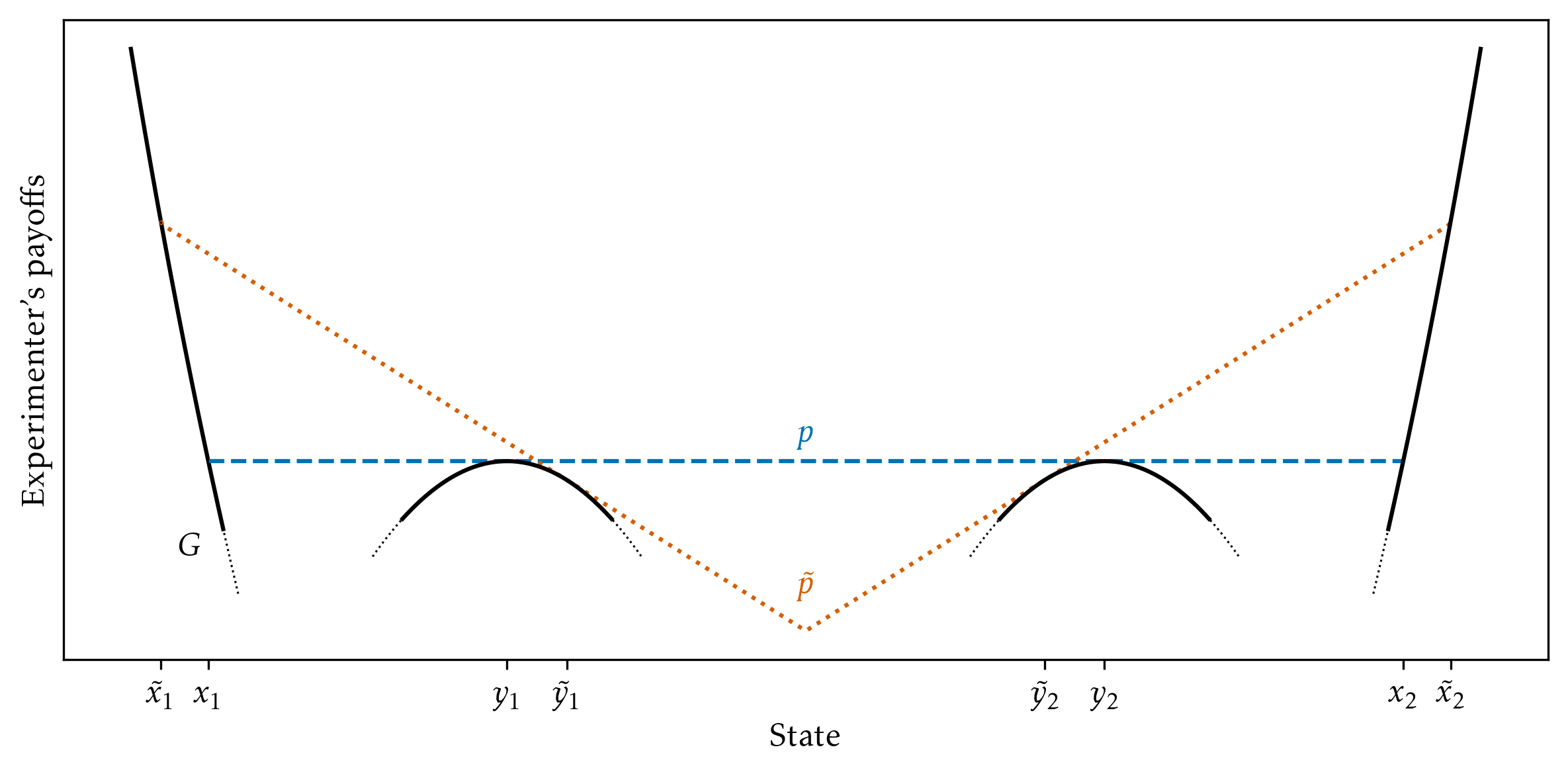
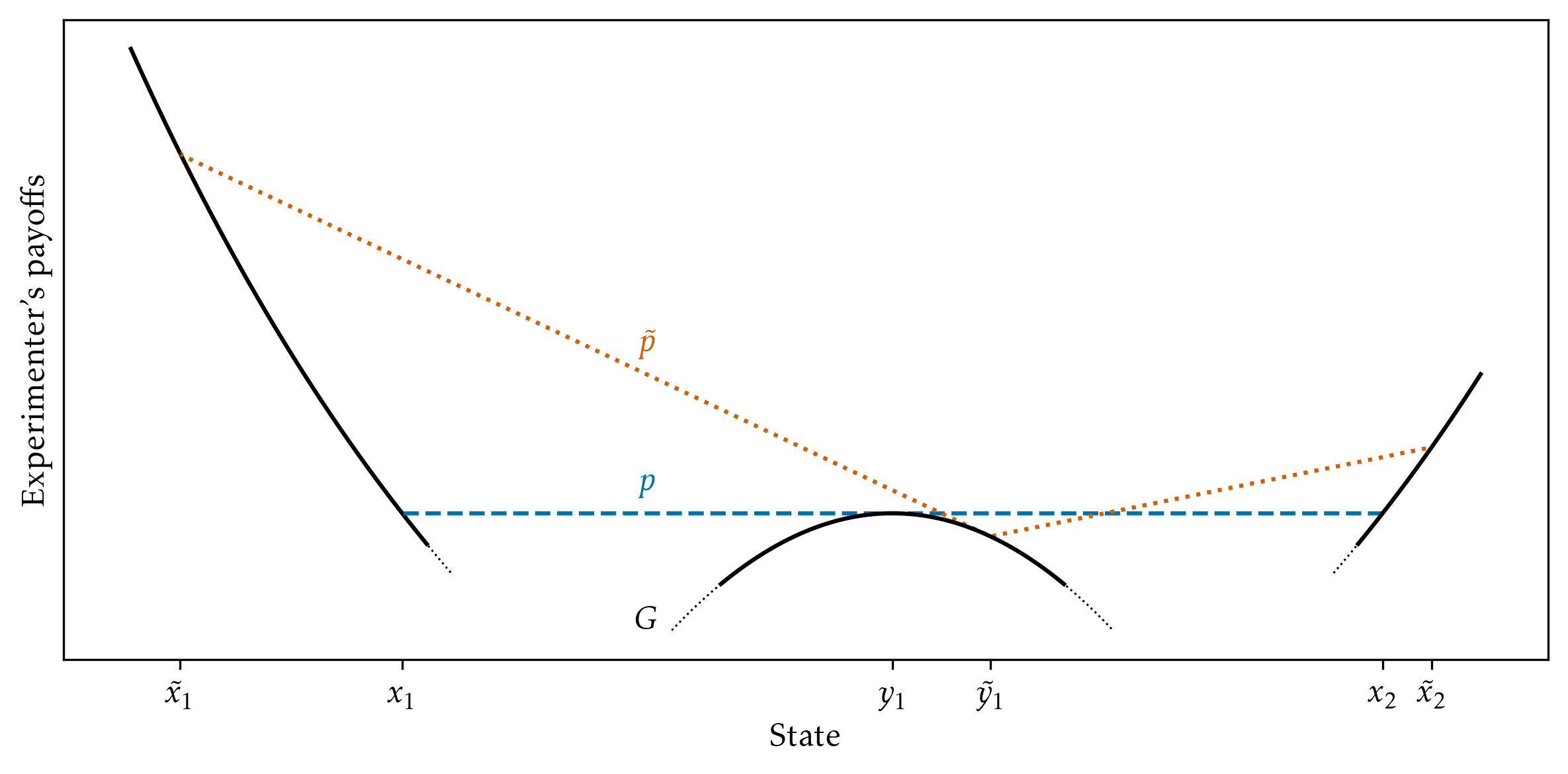
B.1.2 Incomplete full revelation

Incomplete full revelation concerns the extreme points of $\operatorname*{MPC}(H)$. Recall, for each extreme point $F$, there are countably many, disjoint bi-pooling intervals $[x_{1},x_{2}]$, such that $F$ pools $[x_{1},x_{2}]$ to at most two atoms and $I_{F}$ lies strictly below $I_{H}$ on the interior $(x_{1},x_{2})$. Outside the union of the bi-pooling intervals, $I_{F}$ coincides with $I_{H}$. A non-trivial interval $[a,b]$ is fully revealing if $I_{F}$ coincides with $I_{H}$ on $[a,b]$.

Note carefully that full revelation intervals are non-trivial by definition. An extreme point need not admit any full revelation intervals.

Definition 6.

An extreme point $F$ of $\operatorname*{MPC}(H)$ admits incomplete full revelation if there is a non-degenerate bi-pooling interval $[x_{1},x_{2}]$ of $F$ and $\delta>0$ satisfying at least one of the following:

1. $F$ admits two atoms on $(x_{1},x_{2})$, both $[x_{1}-\delta,x_{1}]$ and $[x_{2},x_{2}+\delta]$ are full revelation intervals, and $0<x_{1}<x_{2}<1$ holds.

2. $F$ admits exactly one atom on $(x_{1},x_{2})$, and at least one of the following holds:

   1. Both $[x_{1}-\delta,x_{1}]$ and $[x_{2},x_{2}+\delta]$ are full revelation intervals, and $0<x_{1}<x_{2}<1$ holds.

   2. $[x_{1}-\delta,x_{1}]$ is a full revelation interval, and $0<x_{1}<x_{2}=1$ holds.

   3. $[x_{2},x_{2}+\delta]$ is a full revelation interval, and $0=x_{1}<x_{2}<1$ holds.

In words, $F$ fully reveals the state on non-degenerate intervals to the left and right of a bi-pooling interval (cases (1) and (2a)). Cases (2b) and (2c) are as (2a), except that one neighboring interval is the boundary of the state space.

B.2 Profitable Restrictions

Say full delegation is not optimal if there does not exist optimal $F\in\operatorname*{BR}(H)$.

There exists an extreme point of $\operatorname*{MPC}(H)$ that is designer-preferred among $\operatorname*{BR}(H)$. We refer to such an extreme point as a DEF (designer-optimal extreme point under full delegation). We provide sufficient conditions such that a given DEF is not an optimal IC experiment; accordingly, full delegation is not optimal.

Theorem 4.

Let the designer’s payoff $u_{D}$ be continuously differentiable and strictly convex, let the experimenter’s payoff $u_{E}$ be continuously differentiable, and let the prior $H$ admit a strictly positive density. If the experimenter has locally strict curvature preferences and there exists a DEF with incomplete full revelation, then full delegation is not optimal.

Proof of Theorem˜4.

Let $F$ be a DEF with incomplete full information. Let $\delta>0$ and $[x_{1},x_{2}]$ be as in the definition of incomplete full information. Let $y_{1}$ and $y_{2}$ be the atoms in $[x_{1},x_{2}]$ (possibly $y_{1}=y_{2}$).

Find a price function $p$ as in Corollary 1 of Dworczak and Martini (2019), i.e. $p$ is convex and continuous, and it holds $p\geq G$, $\operatorname*{supp}F\subseteq\{m\in[0,1]\colon p(m)=G(m)\}$ and $\intop\nolimits p\mathop{}\!\mathrm{d}F=\intop\nolimits p\mathop{}\!\mathrm{d}H$. Since $[x_{1},x_{2}]$ is bi-pooling, Corollary 3 of Arieli et al. (2023) tells us that $p$ is affine on $[x_{1},x_{2}]$.

We distinguish the cases of Definition˜6 concerning the form of $[x_{1},x_{2}]$. In all cases, the proof strategy is to use Definition˜5 to find a price function $\tilde{p}$ that touches $G$ close to points at which $p$ equals $G$. Using the price-theoretic characterization of IC, we obtain a particular IC experiment $\tilde{F}$ whose support is close to the support of $F$. For the particularly constructed experiment, we show the designer is strictly better off than under $F$, which completes the proof.

Case 1. $F$ admits two atoms, $y_{1}<y_{2}$, on $(x_{1},x_{2})$, both $[x_{1}-\delta,x_{1}]$ and $[x_{2},x_{2}+\delta]$ are full revelation intervals, and $0<x_{1}<x_{2}<1$ holds.

Since $p$ is affine on $[x_{1},x_{2}]$ and $y_{1},y_{2}\in(x_{1},x_{2})$, both $y_{1}$ and $y_{2}$ must be in the interior of $\mathcal{I}_{\operatorname*{ccv}}$ (in view of Definition˜5). Also, since $I_{F}=I_{H}$ on $[x_{1}-\delta,x_{1}]\cup[x_{2},x_{2}+\delta]$, the functions $p$ and $G$ agree on this set; in particular, $G$ is convex on this set. Thus, $[x_{1}-\delta,x_{1}]\cup[x_{2},x_{2}+\delta]\subseteq\mathcal{I}_{\operatorname*{cvx}}$. Consequently, the tuple $(x_{1},y_{1},y_{2},x_{2})$ meets the hypothesis of Definition˜5. Let $\tilde{T}=(\tilde{x}_{1},\tilde{y}_{1},\tilde{y}_{2},\tilde{x}_{2})$ be as in Definition˜5; for all $r\in(0,1]$, let $\tilde{p}(\cdot,r)$ be a supporting price function.

Throughout, we take $r$ sufficiently close to $0$ such that $\tilde{x}_{1}(r)\in[x_{1}-\delta,x]$ and $\tilde{x}_{2}(r)\in[x_{2},x_{2}+\delta]$, which is possible by continuity of $\tilde{T}$.

The function $\tilde{p}(\cdot,r)$ obtained from Definition˜5 has domain $[\tilde{x}_{1}(r),\tilde{x}_{2}(r)]$. We extend to $[0,1]$ by setting $\tilde{p}(m,r)=p(m)$ for all $m\notin[\tilde{x}_{1}(r),\tilde{x}_{2}(r)]$. The resulting function clearly lies above $G$. One may verify that $\tilde{p}(\cdot,r)$ is convex by observing that $\tilde{p}(\cdot,r)$ lies above $G$ on $[\tilde{x}_{1}(r),\tilde{x}_{2}(r)]$, while $\tilde{x}_{1}(r)$ and $\tilde{x}_{2}(r)$, respectively, lie in the intervals $[x_{1}-\delta,x_{1}]$ and $[x_{2},x_{2}+\delta]$, respectively, on which $p$ coincides with $G$.

We claim $\tilde{y}_{1}^{\prime}(0)>0$ and $\tilde{y}_{2}^{\prime}(0)<0$. Indeed, for small $r$ we have $\tilde{y}_{1}(r),\tilde{y}_{2}(r)\in\mathcal{I}_{\operatorname*{ccv}}$ since $y_{1}$ and $y_{2}$ are in the interior of $\mathcal{I}_{\operatorname*{ccv}}$. The points $(y_{1},G(y_{1}))$ and $(y_{2},G(y_{2}))$ in $\mathbb{R}^{2}$ lie on the graph of an affine function with slope $g(y_{1})=g(y_{2})$. Thus, for $\tilde{T}(r)$ to be supported by a convex price function, concavity of $G$ around $y_{1}$ and $y_{2}$ requires $\tilde{y}_{1}(r)\geq y_{1}$ and $\tilde{y}_{2}(r)\leq y_{2}$ for sufficiently small $r$. Since $\tilde{y}_{1}$ and $\tilde{y}_{2}$ are assumed to be continuously differentiable with non-zero derivatives at $r=0$, we conclude $\tilde{y}_{1}^{\prime}(0)>0$ and $\tilde{y}_{2}^{\prime}(0)<0$.

Figure˜7 schematically depicts the assumed and derived properties of $p$ and $\tilde{p}(\cdot,r)$ for some fixed $r$.

Let $q$ be the constant slope of $I_{F}$ on $(y_{1},y_{2})$, i.e. $q=F(y_{1})$. Since $[x_{1},x_{2}]$ is bi-pooling with atoms $y_{1}$ and $y_{2}$, both $i\in\{1,2\}$ satisfy

$$I_{H}(x_{i})+H(x_{i})(y_{i}-x_{i})=I_{F}(y_{i})+q(y_{i}-y_{i}),$$

where the right side of course simply equals $I_{F}(y_{i})$. The function $t\mapsto I_{H}(t)+H(t)(y_{i}-t)$ has a non-zero derivative at $t=x_{i}$. Therefore, for sufficiently small $r$ the Inverse Function Theorem yields $\tilde{t}_{i}(r)$ such that

$$I_{H}(\tilde{t}_{i}(r))+H(\tilde{t}_{i}(r))(\tilde{y}_{i}(r)-\tilde{t}_{i})=I_{F}(y_{i})+q(\tilde{y}_{i}(r)-y_{i}),$$ (9)

Moreover, $\tilde{t}_{i}(r)\to x_{i}$ as $r\to 0$, and $\tilde{t}_{i}(r)$ is differentiable with respect to $r$, with

$$\tilde{t}_{i}^{\prime}(0)=\tilde{y}_{i}^{\prime}(0)\frac{q-H(x_{i})}{h(x_{i})(y_{i}-x_{i})}.$$

We have $\tilde{t}_{1}^{\prime}(0)>0$ and $\tilde{t}_{2}^{\prime}(0)<0$ since $\tilde{y}_{1}^{\prime}(0)>0$ and $\tilde{y}_{2}^{\prime}(0)<0$ and $x_{1}<y_{1}$ and $y_{2}<x_{2}$. Finally, note that since $I_{F}$ is affine on $[y_{1},y_{2}]$, the right side of (9) simply equals $I_{F}(\tilde{y}_{i}(r))$, for all $r$.

Using $(\tilde{t}_{1}(r),\tilde{x}_{1}(r),\tilde{t}_{2}(r),\tilde{x}_{2}(r))\to(x_{1},x_{1},x_{2},x_{2})$ as $r\to 0$, an application of the Intermediate Value Theorem shows that for $r$ sufficiently small there exist $\tilde{s}_{1}(r)\leq\tilde{x}_{1}(r)$ and $\tilde{s}_{2}(r)\geq\tilde{x}_{2}(r)$ such that

$$\intop\nolimits_{[\tilde{s}_{1}(r),\tilde{t}_{1}(r)]}(\tilde{x}_{1}(r)-\omega)\mathop{}\!\mathrm{d}H(\omega)=\intop\nolimits_{[\tilde{t}_{2}(r),\tilde{s}_{2}(r)]}(\tilde{x}_{2}(r)-\omega)\mathop{}\!\mathrm{d}H(\omega)=0,$$ (10)

i.e. $\tilde{x}_{1}(r)$ is the expectation with respect to $H$ conditional on $[\tilde{s}_{1},\tilde{t}_{2}(r)]$, and likewise for $\tilde{x}_{2}(r)$. We have $\tilde{s}_{1}(r)\to x_{1}$ and $\tilde{s}_{2}(r)\to x_{2}$ as $r\to 0$. The equations (10) imply

$$\forall i\in\{1,2\},\quad I_{H}(\tilde{s}_{i}(r))+H(\tilde{s}_{i}(r))(\tilde{x}_{i}(r)-\tilde{s}_{i}(r))=I_{H}(\tilde{t}_{i}(r))+H(\tilde{t}_{i}(r))(\tilde{x}_{i}(r)-\tilde{t}_{i}(r)).$$

In what follows, fix $r$ sufficiently small such that $\tilde{s}_{1}(r),\tilde{t}_{1}(r),\tilde{t}_{2}(r)$, and $\tilde{s}_{2}(r)$ are well-defined, and $x_{1}-\delta<\tilde{s}_{1}(r)<\tilde{x}_{1}(r)<\tilde{t}_{1}(r)<\tilde{y}_{1}(r)<\tilde{y}_{2}(r)<\tilde{t}_{2}(r)<\tilde{x}_{2}(r)<\tilde{s}_{2}(r)<x_{2}+\delta$.

We define an experiment $\tilde{F}_{r}$ via its integrated CDF, $I_{\tilde{F}_{r}}$. For all $m\in[0,1]$, let

$$I_{\tilde{F}_{r}}(m)=\begin{cases}I_{F}(m)\quad&\mbox{if }m\notin[\tilde{s}_{1}(r),\tilde{s}_{2}(r)],\\ I_{H}(\tilde{s}_{1}(r))+H(\tilde{s}_{1}(r))(m-\tilde{s}_{1}(r))\quad&\mbox{if }m\in[\tilde{s}_{1}(r),\tilde{x}_{1}(r)],\\ I_{H}(\tilde{t}_{1}(r))+H(\tilde{t}_{1}(r))(m-\tilde{t}_{1}(r))\quad&\mbox{if }m\in(\tilde{x}_{1}(r),\tilde{y}_{1}(r)],\\ I_{F}(m)\quad&\mbox{if }m\in(\tilde{y}_{1}(r),\tilde{y}_{2}(r)],\\ I_{H}(\tilde{t}_{2}(r))+H(\tilde{t}_{2}(r))(m-\tilde{t}_{2}(r))\quad&\mbox{if }m\in(\tilde{y}_{2}(r),\tilde{x}_{2}(r)],\\ I_{H}(\tilde{s}_{2}(r))+H(\tilde{s}_{2}(r))(m-\tilde{s}_{2}(r))\quad&\mbox{if }m\in(\tilde{x}_{2}(r),\tilde{s}_{2}(r)].\end{cases}$$

The choice of $(\tilde{s}_{1}(r),\tilde{t}_{1}(r),\tilde{t}_{2}(r),\tilde{s}_{2}(r))$ in (9) and (10) ensures that $\tilde{F}_{r}$ is an experiment, where we recall that $I_{F}$ is affine on $(y_{1},y_{2})$ and given by the right side of (9). Lemma˜2 implies that $\tilde{F}_{r}$ is IC since $\operatorname*{supp}\tilde{F}_{r}\subseteq\{m\in[0,1]\colon\tilde{p}(m,r)=G(m)\}$.

We show that the designer strictly prefers $\tilde{F}_{r}$ to $F$ for $r$ sufficiently small. The designer’s utility from $\tilde{F}_{r}$ is given by

$$\intop\nolimits_{x_{1}-\delta}^{\tilde{s}_{1}(r)}u_{D}(\omega)\mathop{}\!\mathrm{d}H(\omega)+(H(\tilde{t}_{1}(r))-H(\tilde{s}_{1}(r)))u_{D}(\tilde{x}_{1}(r))+(q-H(\tilde{t}_{1}(r)))u_{D}(\tilde{y}_{1}(r))$$ (11)

$$+(H(\tilde{t}_{2}(r))-q)u_{D}(\tilde{y}_{2}(r))+(H(\tilde{s}_{2}(r))-H(\tilde{t}_{2}(r)))u_{D}(\tilde{x}_{2}(r))+\intop\nolimits_{\tilde{s}_{2}(r)}^{x_{2}+\delta}u_{D}(\omega)\mathop{}\!\mathrm{d}H(\omega)$$ (12)

$$+\intop\nolimits_{[0,1]\setminus[x_{1}-\delta,x_{2}+\delta]}u_{D}(m)\mathop{}\!\mathrm{d}F(m).$$

The designer’s utility from $F$ is given by

$$\intop\nolimits_{x_{1}-\delta}^{x_{1}}u_{D}(\omega)\mathop{}\!\mathrm{d}H(\omega)+(q-H(x_{1}))u_{D}(y_{1})$$ (13)

$$+(H(x_{2})-q)u_{D}(y_{2})+\intop\nolimits_{x_{2}}^{x_{2}+\delta}u_{D}(\omega)\mathop{}\!\mathrm{d}H(\omega)$$ (14)

$$+\intop\nolimits_{[0,1]\setminus[x_{1}-\delta,x_{2}+\delta]}u_{D}(m)\mathop{}\!\mathrm{d}F(m).$$

We claim that for $r$ sufficiently small, the sum in (11) is strictly larger than the sum in (13), and the sum in (12) is strictly larger than the sum in (14). The arguments are similar, so we show only the former. Dividing by $r$, the difference between (11) and (13) is

$$\frac{(u_{D}(\tilde{y}_{1}(r))-u_{D}(y_{1}))}{r}(q-H(x_{1}))+(u_{D}(y_{1})-u_{D}(\tilde{x}_{1}(r)))\frac{(H(x_{1})-H(\tilde{t}_{1}(r)))}{r}$$ (15)

$$+\frac{1}{r}\intop\nolimits_{[\tilde{s}_{1}(r),x_{1}]}(u_{D}(\tilde{x}_{1}(r))-u_{D}(\omega))\mathop{}\!\mathrm{d}H(\omega)$$ (16)

As $r\to 0$, the sum of the two terms in (15) converges to

$$\tilde{y}_{1}^{\prime}(0)\mathopen{}\mathclose{{\left(u_{D}^{\prime}(y_{1})(q-H(x_{1}))-(u_{D}(y_{1})-u_{D}(x_{1}))h(x_{1})\tilde{t}_{1}^{\prime}(0)}}\right)$$

$$= \tilde{y}_{1}^{\prime}(0)\mathopen{}\mathclose{{\left(u_{D}^{\prime}(y_{1})-\frac{u_{D}(y_{1})-u_{D}(x_{1})}{y_{1}-x_{1}}}}\right)(q-H(x_{1})).$$

This limit is strictly positive since $u_{D}$ is strictly convex and since $\tilde{y}_{1}^{\prime}(0)>0$ holds. Turning to the integral in (16), find $L>0$ such that $|u_{D}^{\prime}|\leq L$, which is possible since $u_{D}$ is continuously differentiable. Using the choice of $\tilde{s}_{1}(r)$ as per (10), and since $x_{1}\leq\tilde{t}_{1}(r)$ holds, we have

$$\frac{1}{r}\intop\nolimits_{[\tilde{s}_{1}(r),x_{1}]}(u_{D}(\tilde{x}_{1}(r))-u_{D}(\omega))\mathop{}\!\mathrm{d}H(\omega) \geq\frac{-L}{r}\mathopen{}\mathclose{{\left|\intop\nolimits_{[\tilde{s}_{1}(r),x_{1}]}(\tilde{x}_{1}(r)-\omega)\mathop{}\!\mathrm{d}H(\omega)}}\right|$$

$$=\frac{-L}{r}\mathopen{}\mathclose{{\left|\intop\nolimits_{[x_{1},\tilde{t}_{1}(r)]}(\tilde{x}_{1}(r)-\omega)\mathop{}\!\mathrm{d}H(\omega)}}\right|$$

$$\geq\frac{-L}{r}\mathopen{}\mathclose{{\left|\tilde{x}_{1}(r)-x_{1}}}\right|\mathopen{}\mathclose{{\left(H(\tilde{t}_{1}(r))-H(x_{1})}}\right).$$

This lower bound vanishes as $r\to 0$ since $\tilde{x}_{1}(r)\to x_{1}$ and $\tilde{t}_{1}(r)\to x_{1}$ as $r\to 0$, and since $\tilde{t}_{1}(r)$ is differentiable at $r=0$. Therefore, the sum of (15) and (16) is strictly positive for $r$ sufficiently close to $0$.

Case 2. $F$ admits exactly one atom $y_{1}$ on $(x_{1},x_{2})$, both $[x_{1}-\delta,x_{1}]$ and $[x_{2},x_{2}+\delta]$ are full revelation intervals, and $0<x_{1}<x_{2}<1$ holds.

Similarly to the previous case, we have $y_{1}\in\operatorname*{int}\mathcal{I}_{\operatorname*{ccv}}$, and $[x_{1}-\delta,x_{1}]\cup[x_{2},x_{2}+\delta]\subseteq\mathcal{I}_{\operatorname*{cvx}}$. Thus, the tuple $(x_{1},y_{1},y_{1},x_{2})$ meets the hypothesis of Definition˜5. Let $\tilde{T}=(\tilde{x}_{1},\tilde{y}_{1},\tilde{y}_{2},\tilde{x}_{2})$ be as postulated by Definition˜5. For all $r\in(0,1]$, let $\tilde{p}(\cdot,r)$ be a supporting price function. The component $\tilde{y}_{2}(r)$ shall be irrelevant for our argument.

Recall that $\tilde{y}_{1}$ is continuously differentiable with non-zero derivative at $r=0$. Without loss, let $\tilde{y}_{1}^{\prime}(0)>0$, the other case being similar.

Throughout, take $r$ sufficiently small such that $\tilde{y}_{1}(r)>y_{1}$ and $\tilde{x}_{1}(r)\in[x_{1}-\delta,x_{1}]$ and $\tilde{x}_{2}(r)\in[x_{2},x_{2}+\delta]$, where we recall that $\tilde{x}_{1}(r)\leq x_{1}$ and $\tilde{x}_{2}(r)\geq x_{2}$ follow directly from Definition˜5.

Figure˜8 schematically depicts the assumed and derived properties of $p$ and $\tilde{p}(\cdot,r)$ for some fixed $r$.

As in the proof for the previous case, we extend $\tilde{p}(\cdot,r)$ to $[0,1]$ by setting $\tilde{p}(m,r)=p(m)$ for all $m\notin[\tilde{x}_{1}(r),\tilde{x}_{2}(r)]$. The resulting function is continuous, convex, and lies above $G$.

Also similar to the previous case, we proceed by constructing three thresholds $\tilde{s}_{1}(r),\tilde{t}_{1}(r),\tilde{s}_{2}(r)$. (The reader is invited to think of the fourth threshold $\tilde{t}_{2}(r)$ from the previous case as being fixed to $x_{2}$.) Note, it holds

$$I_{H}(x_{1})+H(x_{1})(y_{1}-x_{1})=I_{H}(x_{2})+H(x_{2})(y_{1}-x_{2}),$$

and the function $t\mapsto I_{H}(t)+H(t)(y_{1}-t)$ has a strictly positive derivative at $x_{1}$. Therefore, an application of the Inverse Function Theorem shows that for $r$ sufficiently small there exists $\tilde{t}_{1}(r)$ such that

$$I_{H}(\tilde{t}_{1}(r))+H(\tilde{t}_{1}(r))(\tilde{y}_{1}(r)-\tilde{t}_{1}(r)) =I_{H}(x_{2})+H(x_{2})(\tilde{y}_{1}(r)-x_{2})$$

$$\Leftrightarrow\quad\intop\nolimits_{[\tilde{t}_{1}(r),x_{2}]}(\tilde{y}_{1}(r)-\omega)\mathop{}\!\mathrm{d}H(\omega) =0.$$

Moreover, $\tilde{t}_{1}(r)\to x_{1}$ as $r\to 0$, and $\tilde{t}_{1}(r)$ is differentiable with respect to $r$, with

$$\tilde{t}_{1}^{\prime}(0)=\tilde{y}_{1}^{\prime}(0)\frac{H(x_{2})-H(x_{1})}{h(x_{1})(y_{1}-x_{1})}.$$

Note $\tilde{t}_{1}^{\prime}(0)>0$ since $\tilde{y}_{1}^{\prime}(0)>0$ and $x_{1}<y_{1}<x_{2}$.

Using $(\tilde{x}_{1}(r),\tilde{t}_{1}(r),\tilde{x}_{2}(r))\to(x_{1},x_{1},x_{2})$ as $r\to 0$ and $\tilde{x}_{1}(r)\leq x_{1}<\tilde{t}_{1}(r)$ and $x_{2}\leq\tilde{x}_{2}(r)$, an application of the Intermediate Value Theorem shows that for $r$ sufficiently small there exist $\tilde{s}_{1}(r)$ and $\tilde{s}_{2}(r)$ such that

$$\intop\nolimits_{[\tilde{s}_{1}(r),\tilde{t}_{1}(r)]}(\tilde{x}_{1}(r)-\omega)\mathop{}\!\mathrm{d}H(\omega)\intop\nolimits_{[x_{2},\tilde{s}_{2}(r)]}(\tilde{x}_{2}(r)-\omega)\mathop{}\!\mathrm{d}H(\omega)=0.$$ (17)

We have $\tilde{s}_{1}(r)\leq\tilde{x}_{1}(r)$ and $\tilde{x}_{2}(r)\leq\tilde{s}_{2}(r)$. Moreover, $\tilde{s}_{1}(r)\to x_{1}$ and $\tilde{s}_{2}(r)\to x_{2}$ as $r\to 0$. The equations (17) are equivalent to

$$I_{H}(\tilde{s}_{1}(r))+H(\tilde{s}_{1}(r))(\tilde{x}_{1}(r)-\tilde{s}_{1}(r)) =I_{H}(\tilde{t}_{1}(r))+H(\tilde{t}_{1}(r))(\tilde{x}_{1}(r)-\tilde{t}_{1}(r)),$$

$$I_{H}(x_{2})+H(x_{2})(\tilde{x}_{2}(r)-x_{2}) =I_{H}(\tilde{s}_{2}(r))+H(\tilde{s}_{2}(r))(\tilde{x}_{1}(r)-\tilde{s}_{2}(r))$$

Define the experiment $\tilde{F}_{r}$ via its integrated CDF as follows:

$$\forall m\in[0,1]\quad I_{\tilde{F}_{r}}(m)=\begin{cases}I_{F}(m)\quad&\mbox{if }m\notin[\tilde{s}_{1}(r),\tilde{s}_{2}(r)],\\ I_{H}(\tilde{s}_{1}(r))+H(\tilde{s}_{1}(r))(m-\tilde{s}_{1}(r))\quad&\mbox{if }m\in[\tilde{s}_{1}(r),\tilde{x}_{1}(r)],\\ I_{H}(\tilde{t}_{1}(r))+H(\tilde{t}_{1}(r))(m-\tilde{t}_{1}(r))\quad&\mbox{if }m\in(\tilde{x}_{1}(r),\tilde{y}_{1}(r)],\\ I_{H}(x_{2})+H(x_{2})(m-x_{2})\quad&\mbox{if }m\in(\tilde{y}_{1}(r),\tilde{x}_{2}(r)],\\ I_{H}(\tilde{s}_{2}(r))+H(\tilde{s}_{2}(r))(m-\tilde{s}_{2}(r))\quad&\mbox{if }m\in(\tilde{x}_{2}(r),\tilde{s}_{2}(r)].\end{cases}$$

The choice of $\tilde{t}_{1}(r)$, $\tilde{s}_{1}(r)$, and $\tilde{s}_{2}(r)$ ensure that $\tilde{F}_{r}$ is an experiment. Lemma˜2 implies that $\tilde{F}_{r}$ is IC since $\operatorname*{supp}\tilde{F}_{r}\subseteq\{m\in[0,1]\colon\tilde{p}(m,r)=G(m)\}$. We show the designer is strictly better off under $\tilde{F}_{r}$ than $F$ for $r$ sufficiently small.

The designer’s utility from $\tilde{F}_{r}$, denoted $U_{D}(\tilde{F}_{r})$, is given by

$$U_{D}(\tilde{F}_{r})=(H(\tilde{t}_{1}(r))-H(\tilde{s}_{1}(r)))u_{D}(\tilde{x}_{1}(r))+(H(x_{2})-H(\tilde{t}_{1}(r)))u_{D}(\tilde{y}_{1}(r))$$

$$+(H(\tilde{s}_{2}(r))-H(x_{2}))u_{D}(\tilde{x}_{2}(r))+\intop\nolimits_{[0,1]\setminus[\tilde{s}_{1}(r),\tilde{s}_{2}(r)]}u_{D}(m)\mathop{}\!\mathrm{d}F(m)$$

The designer’s utility from $F$, denoted $U_{D}(F)$, is given by

$$U_{D}(F)=(H(x_{2})-H(x_{1}))u_{D}(y_{1})+\intop\nolimits_{[\tilde{s}_{1}(r),x_{1}]}u_{D}(\omega)\mathop{}\!\mathrm{d}H(\omega)$$

$$+\intop\nolimits_{[x_{2},\tilde{s}_{2}(r)]}u_{D}(\omega)\mathop{}\!\mathrm{d}H(\omega)+\intop\nolimits_{[0,1]\setminus[\tilde{s}_{1}(r),\tilde{s}_{2}(r)]}u_{D}(m)\mathop{}\!\mathrm{d}F(m).$$

The difference $\frac{1}{r}(U_{D}(\tilde{F}_{r})-U_{D}(F))$ equals

$$(H(x_{2})-H(x_{1}))\frac{u_{D}(\tilde{y}_{1}(r))-u_{D}(y_{1})}{r}+\frac{(H(x_{1})-H(\tilde{t}_{1}(r)))}{r}(u_{D}(\tilde{y}_{1}(r))-u_{D}(\tilde{x}_{1}(r)))$$ (18)

$$+\frac{1}{r}\intop\nolimits_{[\tilde{s}_{1}(r),x_{1}]}(u_{D}(\tilde{x}_{1}(r))-u_{D}(\omega))\mathop{}\!\mathrm{d}H(\omega)$$ (19)

$$+\frac{1}{r}\intop\nolimits_{[x_{2},\tilde{s}_{2}(r)]}(u_{D}(\tilde{x}_{2}(r))-u_{D}(\omega))\mathop{}\!\mathrm{d}H(\omega).$$ (20)

We argue that, as $r\to 0$, the sum in (18) converges to a strictly positive term, whereas both (19) and (20) admit vanishing lower bounds.

The limit of (18) as $r\to 0$ equals

$$\mathopen{}\mathclose{{\left(H(x_{2})-H(x_{1})}}\right)\tilde{y}_{1}^{\prime}(0)\mathopen{}\mathclose{{\left(u_{D}^{\prime}(y_{1})-\frac{u_{D}(y_{1})-u_{D}(x_{1})}{y_{1}-x_{1}}}}\right).$$

This limit is strictly positive since $u_{D}$ is strictly convex and $\tilde{y}_{1}^{\prime}(0)>0$.

Now consider (19). Find $L>0$ such that $|u_{D}^{\prime}|\leq L$. Using the choice of $\tilde{s}_{1}(r)$ in (17) and $x_{1}\leq\tilde{t}_{1}(r)$, we have

$$\frac{1}{r}\intop\nolimits_{[\tilde{s}_{1}(r),x_{1}]}(u_{D}(\tilde{x}_{1}(r))-u_{D}(\omega))\mathop{}\!\mathrm{d}H(\omega)\geq \frac{-L}{r}\mathopen{}\mathclose{{\left|\intop\nolimits_{[\tilde{s}_{1}(r),x_{1}]}(\tilde{x}_{1}(r)-\omega)\mathop{}\!\mathrm{d}H(\omega)}}\right|$$

$$= \frac{-L}{r}\mathopen{}\mathclose{{\left|\intop\nolimits_{[x_{1},\tilde{t}_{1}(r)]}(\tilde{x}_{1}(r)-\omega)\mathop{}\!\mathrm{d}H(\omega)}}\right|$$

$$\geq \frac{-L}{r}\mathopen{}\mathclose{{\left|(\tilde{x}_{1}(r)-x_{1})(H(\tilde{t}_{1}(r))-H(x_{1}))}}\right|.$$

The ratio $\frac{1}{r}(\tilde{x}_{1}(r)-x_{1})$ converges to $\tilde{x}_{1}^{\prime}(0)$ as $r\to 0$ (since $\tilde{x}_{1}$ is differentiable at $r=0$, by Definition˜5). Meanwhile, $H(\tilde{t}_{1}(r))-H(x_{1})$ vanishes as $r\to 0$. Thus, (19) admits a vanishing lower bound.

Now consider (20). Using the choice of $\tilde{s}_{2}(r)$ in (17), we have

$$\frac{1}{r}\intop\nolimits_{[x_{2},\tilde{s}_{2}]}(u_{D}(\tilde{x}_{2}(r))-u_{D}(\omega))\mathop{}\!\mathrm{d}H(\omega)\geq \frac{-L}{r}\mathopen{}\mathclose{{\left|\intop\nolimits_{[x_{2},\tilde{s}_{2}(r)]}(\tilde{x}_{2}(r)-\omega)\mathop{}\!\mathrm{d}H(\omega)}}\right|$$

$$= \frac{-L}{r}\mathopen{}\mathclose{{\left|(x_{2}-\tilde{x}_{2}(r))(H(\tilde{s}_{2}(r))-H(x_{2}))}}\right|.$$

The ratio $\frac{1}{r}(x_{2}-\tilde{x}_{2}(r))$ converges to $\tilde{x}_{2}^{\prime}(0)$ as $r\to 0$ (Definition˜5), while $H(\tilde{s}_{2}(r))-H(x_{2})$ vanishes as $r\to 0$. Thus, (20) admits a vanishing lower bound.

Case 3. $F$ admits exactly one atom $y_{1}$ on $(x_{1},x_{2})$, the interval $[x_{1}-\delta,x_{1}]$ is a full revelation interval, and $0<x_{1}<x_{2}=1$ holds.

The proof is similar to the proof of Theorem˜2, and hence we shall be brief. Abbreviate $y=y_{1}$ and $x=x_{1}$. As before, $y\in\operatorname*{int}\mathcal{I}_{\operatorname*{ccv}}$, and $[x-\delta,x]\subseteq\mathcal{I}_{\operatorname*{cvx}}$. In this case, the price $p$ is affine on $[x,1]$; in particular, $G(x)+g(y)(y-x)=G(y)$. For $\tilde{y}$ converging to $y$ from above, consider the affine function $t\mapsto G(\tilde{y})+g(\tilde{y})(t-\tilde{y})$. For $\tilde{y}$ close to $y$, this affine function intersects $G$ at a point $\tilde{x}$ in $[x-\delta,x]$ since $y\in\operatorname*{int}\mathcal{I}_{\operatorname*{ccv}}$, and $[x-\delta,x]\subseteq\mathcal{I}_{\operatorname*{cvx}}$. Consider the function $\tilde{p}$ that coincides with $p$ up to $\tilde{x}$, then equals the affine function up to $\tilde{y}$, and finally continues with a sufficiently steep slope such that $\tilde{p}$ is convex and lies above $G$ on $[\tilde{y},1]$. The function $\tilde{p}$ is convex and lies above $G$ on all of $[0,1]$. Now find $\tilde{t}$ such that $\tilde{y}=\mathbb{E}_{H}[\bm{\omega}\mid\bm{\omega}\in[\tilde{y},1]]$ and $\tilde{x}=\mathbb{E}_{H}[\bm{\omega}\mid\bm{\omega}\in[\tilde{s},\tilde{t}]$, which is possible for $\tilde{y}$ sufficiently close to $y$. Finally, let $\tilde{F}$ be the experiment that coincides with $F$ up to $\tilde{s}$, then pools $H$ on $[\tilde{s},\tilde{t}]$ to $\tilde{x}$, and pools $H$ on $[\tilde{t},1]$ to $\tilde{y}$. For $\tilde{y}$ sufficiently close to $y$, the point $\tilde{s}$ is in $[x-\delta,x]$, implying that $\tilde{F}$ is supported on points $m$ such that $\tilde{p}(m)=G(m)$. In particular $\tilde{F}$ is IC. A calculation similar to the one in the proof of Theorem˜2 shows that the designer is strictly better off under $\tilde{F}$ than under $F$.

Case 4. $F$ admits exactly one atom $y_{1}$ on $(x_{1},x_{2})$, the interval $[x_{2},x_{2}+\delta]$ is a full revelation interval, and $0=x_{1}<x_{2}<1$ holds. Analogous to the previous case. ∎

Appendix C Extreme Point Representation

In this appendix, we provide a general extreme point representation of IC experiments. Let $G$ satisfy part (i) of the regularity condition of Dworczak and Martini (2019), as in Section˜6.3; in particular, Lemma˜2 applies.

Let $\nu$ be a Borel probability measure on $\operatorname*{MPC}(H)$, where $\operatorname*{MPC}(H)$ has the $L^{1}$-norm. Let $F\in\operatorname*{MPC}(H)$. Say $\nu$ represents $F$ if $V(F)=\intop\nolimits V(\Phi)\mathop{}\!\mathrm{d}\nu(\Phi)$ holds for all continuous linear functionals $V\colon\operatorname*{MPC}(H)\to\mathbb{R}$. Say $\nu$ is supported on a measurable set $\mathcal{F}\subseteq\operatorname*{MPC}(H)$ if $\nu(\mathcal{F})=1$.

The set of incentive-compatible extreme points of $\operatorname*{MPC}(H)$ is measurable since IC experiments form a closed set (see Section˜A.1) while the extreme points form a $G_{\delta}$-set (Aliprantis and Border (2006, Lemma 7.63)).

Theorem 5.

For all IC experiments $F$ there exists a Borel probability measure $\nu$ that represents $F$ and is supported on the set of incentive-compatible extreme points of $\operatorname*{MPC}(H)$.

The content of Theorem˜5 is that the extreme points can be chosen to be IC, and that they are extreme points of the entire set $\operatorname*{MPC}(H)$.

Theorem˜5 does not imply that the set of IC experiments is convex. Indeed, it is not generally convex: for $S$-shaped preferences of the experimenter, IC experiments can have at most one atom in the concave part of $G$ (Lemma˜3), implying that a proper mixture of two distinct double censorship experiments is not IC.

Proof of Theorem˜5.

Let $F$ be IC. By Lemma˜2, there exists a continuous, convex function $p\colon[0,1]\to\mathbb{R}$ such that $p\geq G$ and $\operatorname*{supp}F\subseteq\{m\in[0,1]\colon p(m)=G(m)\}$. By Choquet’s Representation Theorem (e.g. Phelps (2002) or Kleiner et al. (2021, Proposition 1)), there exists a measure $\nu$ that represents $F$ and is supported on the extreme points of $\operatorname*{MPC}(H)$.

We argue that $\nu$-almost all are IC. We use Lemma˜2. Let $K=\{m\in[0,1]\colon p(m)=G(m)\}$ and $O=[0,1]\setminus K$. The set $K$ is closed and $O$ is open (in $[0,1]$) since $p-G\geq 0$ holds and since $p-G$ is lower semicontinuous.

Let $\gamma$ be a continuous function such that $\gamma(m)>0$ for all $m\in O$ and $\gamma(m)=0$ for all $m\in K$; e.g., let $\gamma(m)=\min_{m^{\prime}\in K}|m-m^{\prime}|$, where the minimum is well-defined and continuous by closedness of $K$ and Berge’s Maximum Theorem. Thus, the linear functional $\Phi\mapsto\intop\nolimits\gamma(m)\mathop{}\!\mathrm{d}\Phi(m)$ is continuous. Since $\nu$ represents $F$ and $\operatorname*{supp}F\subseteq\{m\in[0,1]\colon p(m)=G(m)\}=K$, we have $0=\intop\nolimits\intop\nolimits_{O}\gamma(m)\mathop{}\!\mathrm{d}\Phi(m)\mathop{}\!\mathrm{d}\nu(\Phi)$. Since $\gamma$ is strictly positive on $O$, it follows that $\nu$-almost all assign mass $0$ to the set $O$. Since $[0,1]\setminus O=K=\{m\in[0,1]\colon p(m)=G(m)\}$ and since $K$ is closed, it follows that $\nu$-almost all satisfy $\operatorname*{supp}\Phi\subseteq\{m\in[0,1]\colon p(m)=G(m)\}$. Invoking Lemma˜2 with the price function $p$, it follows that $\nu$-almost all are IC. ∎