TacLoc: Global Tactile Localization on Objects
from a Registration Perspective

Abstract

Pose estimation is essential for robotic manipulation, particularly when visual perception is occluded during gripper-object interactions. Existing tactile-based methods generally rely on tactile simulation or pre-trained models, which limits their generalizability and efficiency. In this study, we propose TacLoc, a novel tactile localization framework that formulates the problem as a one-shot point cloud registration task. TacLoc introduces a graph-theoretic partial-to-full registration method, leveraging dense point clouds and surface normals from tactile sensing for efficient and accurate pose estimation. Without requiring rendered data or pre-trained models, TacLoc achieves improved performance through normal-guided graph pruning and a hypothesis-and-verification pipeline. TacLoc is evaluated extensively on the YCB dataset. We further demonstrate TacLoc on real-world objects across two different visual-tactile sensors.

I Introduction

Global pose estimation is fundamental to robotic autonomy. For mobile robots, global localization methods enable pose estimation from scratch on a known map [35]. For robotic manipulators, global pose estimation involves determining the pose of the object relative to the robot base, which is critical for ensuring the success of subsequent manipulation tasks. When the end effector is in contact with an object, the object pose can be decomposed as:

$$\mathbf{T}_{\text{base}}^{\text{obj}}=\mathbf{T}_{\text{base}}^{\text{ee}}\cdot\mathbf{T}_{\text{ee}}^{\text{obj}}$$ (1)

where $\mathbf{T}_{\text{base}}^{\text{obj}}\in\mathrm{SE}(3)$ denotes the object pose in the robot base frame, $\mathbf{T}_{\text{base}}^{\text{ee}}$ is the end-effector pose in the base frame, readily available through forward kinematics of the manipulator, and $\mathbf{T}_{\text{ee}}^{\text{obj}}$ represents the object pose expressed in the end-effector frame. Since $\mathbf{T}_{\text{base}}^{\text{ee}}$ is known, the core problem reduces to estimating $\mathbf{T}_{\text{ee}}^{\text{obj}}$ from sensory measurements at the end effector.

During manipulation, however, the interactions between the end effector and the object easily occlude visual perception, making tactile sensing an increasingly popular modality for contact-based pose estimation. Tactile-based global localization thus focuses on estimating $\mathbf{T}_{\text{ee}}^{\text{obj}}$ from the first touch. Existing studies [25, 30, 3] typically involve rendering tactile data onto the object model and computing the similarity with real sensing, which essentially serves as a tactile measurement model for estimating the pose distribution. This distribution is then incorporated into a Monte Carlo localization (MCL) framework [30] or used for precise matching [3]. However, these methods rely on well-trained networks for codebook building [30] and rendering [3], which limits their generalization to different types of tactile sensors or new objects. The efficiency of similarity computation is influenced by the discretization resolution of the $\mathfrak{se}(3)$ space. Furthermore, sequential-based estimation might fail if the finger loses contact with the object.

Figure 1: Real-world demonstration using TacLoc. A GelSight Mini sensor touches a textureless 3D-printed object (left), producing a tactile image that is converted into a dense point cloud and registered to a prior CAD model (right). The zoomed view shows the tactile point cloud (blue) aligned on the CAD model (red).

One-shot global localization enables direct pose estimation on a given map without sequential filtering in the mobile robotics community [9, 23], i.e., aligning partial measurements to the full map via global matching, without the similarity comparison. Inspired by this, we aim to answer the question: Is it feasible to achieve one-shot global localization for contact-based tactile sensing? If so, how can it be done? Compared to field-level matching for mobile robots, there are two practical challenges for in-hand tactile-based localization: 1) the tactile sensing is fundamentally different from the object model (CAD); 2) deviations between as-designed models and as-is objects introduce challenges in pose estimation. In this study, we propose a novel registration method for global tactile localization, named TacLoc, to mitigate the impact of the above challenges. Overall, the novelties and contributions can be summarized as follows:

• We explore the feasibility of tactile pose estimation from a point cloud registration perspective, different from relying on rendering or pre-trained models as in existing methods.

• We design a graph-theoretic partial-to-full registration method for global tactile localization. This reduces the number of edges and computation time by approximately $52\%$ and $93\%$, respectively.

• TacLoc is successfully deployed on three different visual-tactile sensors: DIGIT, GelSight, and Daimon. We conduct in-depth analyses on simulated YCB datasets and test TacLoc on 5 real-world household objects, achieving a success rate of 33/50.

II Related Work

We first discuss the related work on tactile-based localization. Following this, we review recent trends in point cloud registration.

II-A Tactile Pose Estimation

Visual-tactile sensors typically provide 2D images on fingers [37, 17]. Early work [20] performed 3 degrees of freedom (DoF) pose estimation by utilizing visual keypoints and applying RANSAC for correspondence estimation, following a typical image matching pipeline. 2D occupancy grid map has also been a basic representation for tactile localization [26].

Robotic manipulation tasks are generally conducted in $\mathrm{SE}(3)$ space, requiring 6 DoF object pose estimation relative to the end effector. Image-to-3D conversion is achieved by recovering depth maps from tactile images [37]. In the robotics community, MCL has emerged as a powerful Bayesian framework for pose estimation at the back end. Petrovskaya and Khatib [25] incorporated MCL for global tactile localization, demonstrating its applicability on five common objects. Specifically, the object model provides expected contact geometries for building an analytical measurement model, i.e., predicting what the object surface should feel like under various touch configurations. Suresh et al.  [30] leveraged a measurement model based on a tactile code network learned from tactile simulation. This model is adapted from LiDAR place recognition [15]. In the work by Bauza et al.  [3], 2D contact shapes are rendered via simulation and compared with real tactile images to compute the pose distribution. Ota et al.  [24] further enhanced particle filtering with an active action-planning strategy, enabling the robot to minimize observation time while efficiently identifying and localizing the peg part in assembly tasks.

The key aspect of the above works is to render or simulate tactile sensing given the object. Subsequently, the rendered images are fed into convolutional neural networks (CNN) [4, 3] or point cloud networks [30] for similarity computation. In this study, the proposed TacLoc achieves tactile pose estimation through one-shot global registration, offering a different perspective compared to existing studies.

Recent advances have also introduced multimodal fusion, where visual inputs provide an initial pose, and tactile sensing refines this estimate while complementing the shape of the object [19, 18]. While multiple sensors offer richer measurements, it falls outside the scope of our study.

II-B Global Point Cloud Registration

Global registration estimates the relative pose between measured point clouds and a given model. It is typically classified into correspondence-free and correspondence-based approaches [35]. Correspondence-free methods are applicable in pseudo-2D settings, such as the branch-and-bound (BnB) approach in [2]. Extending these methods to full 3D scenarios significantly increases computational complexity. For correspondence-based methods, a critical component is the use of local descriptors, like Fast Point Feature Histograms (FPFH) [29], to build correspondences. While learning-based descriptors [1, 27] have shown strong performance, they require large-scale training data and face generalization challenges across different modalities and environments. These challenges are further exacerbated in tactile sensing due to the lack of a well-labeled dataset.

The initial correspondence set derived from descriptors often contains many outliers due to noise or repetitive structures, making effective outlier rejection crucial for accurate transformation estimation. Traditional methods, such as Random Sample Consensus (RANSAC)[11], rely on consensus maximization, but their performance degrades significantly under high outlier ratios. Recent graph-theoretic pruning approaches construct a compatibility graph, where nodes represent correspondences and edges encode mutual consistency. Lusk et al. [22] identified the maximum clique for outlier rejection, while Yang et al.  [34] relaxed the maximum clique to maximal cliques, allowing broader exploration of local consensus for more accurate pose hypotheses. Qiao et al.  [28] relaxed the compatibility graph and proposed a distrust-and-verify scheme to select the best hypotheses. This scheme leveraged both sparse features and dense point clouds for the pose verification.

The proposed TacLoc is inspired by existing studies on global registration [22, 34, 28]. We extract FPFH descriptors from tactile-reconstructed point clouds and design a robust backend for outlier rejection. Specifically, considering the nature of tactile sensing, we introduce a normal-guided graph pruning strategy that enforces sparsity and accelerates the clique search process. The designed pipeline does not require additional training data.

III Problem Formulation

The global localization of mobile robots [35] involves estimating the most probable pose $\mathbf{x}\in\mathrm{SE}(3)$, given observations $\mathbf{z}$ and a known map $\mathbf{m}$. This estimation is typically formulated within the framework of Bayesian inference as follows:

$${\rm p}(\mathbf{x|z,m})\propto\underbrace{{\rm p}(\mathbf{z|x,m})}_{\text{observation}}\cdot\underbrace{{\rm p}(\mathbf{x|m})}_{\text{prior}}$$ (2)

For in-hand tactile localization, $\mathbf{z}$ represents tactile images captured by the sensor, while $\mathbf{m}$ corresponds to the object model that the robot interacts with. For the prior distribution, a common approach involves employing recursive Bayesian filtering [30]. Other approaches [3, 8] avoid explicit priors by assuming a uniform distribution over the entire $\mathrm{SE}(3)$ pose space, thus performing exhaustive search. Regarding the measurement model, it can be formulated based on geometric residuals [25] or derived from place recognition results [30].

Different from the methods above, we model the global localization problem as a one-shot localization problem, without the sequential Bayesian inference. Moreover, we formulate a tactile registration pipeline for one-shot pose estimation, guided by a hypothesis-and-verification scheme, which proceeds as follows:

$${\rm p}(\mathbf{x|z,m}) =\int\underbrace{{\rm p}(\mathbf{x|\boldsymbol{\theta},z,m})}_{\text{verification}}\cdot\underbrace{{\rm p}(\boldsymbol{\theta}|\mathbf{z,m})}_{\text{hypothesis}}\,{\rm d}\boldsymbol{\theta}$$

$$\approx\frac{1}{\sum_{k=1}^{K}w_{k}}\cdot\sum_{k=1}^{K}w_{k}\cdot{\rm p}(\boldsymbol{\theta}_{k})$$ (3)

in which we approximate the posterior via $K$ candidate poses $\{\boldsymbol{\theta}_{k}\}_{k=1}^{K}$ and its corresponding weight term $w_{k}$, i.e., the multiple hypotheses and their confidences. More specifically, the term $\boldsymbol{\theta}_{k}$ is a transformation matrix ${\mathbf{T}}_{k}\in\mathrm{SE}(3)$ in practice; the weight term is estimated in the verification phase. In the proposed TacLoc, the candidate with the maximum likelihood is selected as the final result. More details of the TacLoc are presented in the following section.

IV Methodology

Figure 2: Overview of the TacLoc pipeline for one-shot global tactile localization. The process starts with feature extraction to establish initial correspondences. A compatibility graph is constructed based on distance and normal consistency, and maximal cliques are identified for pose hypothesis generation. Finally, a hypothesis-and-verification approach is applied to refine the pose estimation, achieving partial-to-full tactile localization. It is worth noting that a CAD model is indispensable as a prior map and end-effector poses are required to build submaps during sliding touch.

We introduce TacLoc by following the pose estimation pipeline, which encompasses both front-end processing and back-end estimation. The front end begins with the raw data obtained from the sensor, while the back end concludes with the pose estimation relative to the object frame.

IV-A From Raw Data to Initial Correspondence

For visual-tactile sensors, raw images are initially processed to recover the height map $\mathbf{H}$ and gradient maps $\nabla\mathbf{H}=(\mathbf{G}_{x},\mathbf{G}_{y})$ of the contacted surface. These maps are subsequently converted into point clouds with associated normals to facilitate pose estimation. The method of recovering height maps varies depending on the tactile sensor in use. For instance, the high-resolution DIGIT sensor[17] directly recovers the height map using a fully convolutional residual network[16], and gradient maps are derived via partial differentiation of the height map. In contrast, the GelSight Mini (shown in Figure 1) estimates gradient angle maps $[\tan^{-1}(\mathbf{G}_{x}),\tan^{-1}(\mathbf{G}_{y})]$ using a fully connected neural network that processes five-dimensional features: RGB illumination and XY coordinates. The height map is then computed by solving a Laplacian equation using the discrete cosine transform (DCT) [37]:

$$\Delta\mathbf{H}=\frac{\partial^{2}\mathbf{H}}{\partial x^{2}}+\frac{\partial^{2}\mathbf{H}}{\partial y^{2}}=\frac{\partial{\mathbf{G}}_{x}}{\partial x}+\frac{\partial{\mathbf{G}_{y}}}{\partial y}$$ (4)

in which $\Delta$ is the Laplacian operator. Generally, the height recovery involves learned regressors provided by the SDK.

The points and their associated normals are derived element-wise using the height map and gradient maps. Given end-effector poses (e.g., obtained through forward kinematics from the manipulator), a point cloud submap can be constructed from a sequence of measurements. Alternatively, a single-shot measurement can also be utilized for one-shot pose estimation. To ensure computational efficiency during pose estimation, voxel grid downsampling is applied to the point clouds. Keypoints are then detected using the Intrinsic Shape Signatures (ISS) [38] algorithm and are encoded using FPFH [29] for each keypoint (depicted in Figure 3). Finally, initial correspondences are established by performing Manhattan distance matching in the feature space.

One might argue that learning-based keypoint and descriptor extraction could be a better choice. While we agree that data-driven approaches can improve front-end performance, there are two key considerations: first, there is a lack of publicly available datasets to support learning-based tactile perception, when compared to the extensive datasets available for mobile robots; second, one key contribution of this study is the implementation of the hypothesis-and-verification scheme. We will demonstrate that ISS and FPFH are simple yet effective within this framework.

Figure 3: For each frame captured by the tactile sensor, we first convert it into a point cloud with normals. Then we construct a submap representing either a sliding touch or multi-time retouch by integrating end-effector poses. This submap is then processed using our front-end preprocessing pipeline. Best viewed zoomed in and in color.

IV-B Multiple Pose Hypotheses Generation

We first perform graph-theoretic pruning to refine the initial correspondences. Following this, we solve for maximal cliques within the pruned graph to generate multiple pose hypotheses.

IV-B1 Pairwise Consistency

Given two corresponded feature points, the feature points from the target and source point clouds are denoted as $\mathcal{P}^{\text{tar}}=\{\mathbf{p}_{i}^{\text{tar}}\in\mathbb{R}^{3}\}$ and $\mathcal{P}^{\text{src}}=\{\mathbf{p}_{i}^{\text{src}}\in\mathbb{R}^{3}\}$, respectively. The associated surface normals are denoted as $\mathcal{N}^{\text{tar}}=\{\mathbf{n}_{i}^{\text{tar}}\in\mathbb{R}^{3}\}$ and $\mathcal{N}^{\text{src}}=\{\mathbf{n}_{i}^{\text{src}}\in\mathbb{R}^{3}\}$, respectively. We assume that the interacted object is a rigid body, meaning that its shape and structure remain unchanged during the manipulation. Consequently, the two correspondences are considered pairwise consistent if they satisfy the following three conditions.

Distance Consistency. We set the Euclidean difference between two feature points to remain within bounds $\delta_{d}$ :

$$\left|\lVert\mathbf{p}_{i}^{\text{src}}-{\mathbf{p}}_{j}^{\text{src}}\rVert-\lVert{\mathbf{p}}_{i}^{\text{tar}}-{\mathbf{p}}_{j}^{\text{tar}}\rVert\right|<\delta_{d}$$ (5)

Normal Consistency. Visual-tactile sensing is naturally dense, enabling much more precise surface normal estimation compared to other measurement modalities. We also propose that the absolute angular difference between consistent correspondences lies within a limited range:

$$\left|\angle({\mathbf{n}}_{i}^{\text{src}},{\mathbf{n}}_{j}^{\text{src}})-\angle({\mathbf{n}}_{i}^{\text{tar}},{\mathbf{n}}_{j}^{\text{tar}})\right|<\delta_{\alpha}$$ (6)

Injective Consistency. Each source point can map to at most one target point, and each target point can also map to at most one source point:

$$\forall\,(i,j),\,i\neq j,\quad\mathbf{p}_{i}^{\text{src}}\neq\mathbf{p}_{j}^{\text{src}}\land\mathbf{p}_{i}^{\text{tar}}\neq\mathbf{p}_{j}^{\text{tar}}$$ (7)

IV-B2 Maximal Cliques

A compatibility graph is constructed based on these consistency check criteria above, where nodes represent individual correspondences and edges encode pairwise geometric consistency. Then, maximal cliques are extracted and ranked by size using a modified Bron–Kerbosch algorithm [6]. The graph operations and clique extraction are implemented using the NetworkX library [12]. A fixed number of top cliques are selected for the following pose estimation and verification. Figure 4 shows a case study of the candidate extraction pipeline.

The sparse point clouds reconstructed by range sensing (e.g., laser scanners and radar) often lack sufficient density for consistent normal estimation. In contrast, the dense point clouds obtained from tactile sensors enable robust and accurate normal vector computation. This differs from the distance-only consistency check used in prior methods, such as [28]. It is worth mentioning that 3DMAC [34] also incorporates normal consistency for graph pruning through a condition $|\sin\angle({\mathbf{n}}_{i}^{\text{src}},{\mathbf{n}}_{j}^{\text{src}})-\sin\angle({\mathbf{n}}_{i}^{\text{tar}},{\mathbf{n}}_{j}^{\text{tar}})|<t_{\alpha}$. Our approach differs fundamentally and has superiority in time cost. Specifically, while 3DMAC performs post-hoc normal consistency checks, our method conducts preemptive verification, thus ensuring graph sparsity and reducing the complexity of clique extraction.

(a) Initial Corr.

(b) Graph Constr.

(c) Clique 1

(d) Clique 2

Figure 4: Visualization of candidate extraction pipeline with a minimal example (best viewed in color). (a) Three points in the source point cloud (blue) and three points in the target point cloud (orange), connected by six initial correspondences (gray lines). (b) The correspondences form an undirected graph $G$, with nodes $V=\{\xi_{1,1},\xi_{1,2},\xi_{2,1},\xi_{2,2},\xi_{2,3},\xi_{3,3}\}$ and edges $E=\{\{\xi_{1,1},\xi_{2,2}\},\{\xi_{1,1},\xi_{3,3}\},\{\xi_{1,2},\xi_{2,1}\},\{\xi_{2,2},\xi_{3,3}\}$, constructed via pairwise consistency checks. (c) The first maximal clique $C_{1}=\{\xi_{1,1},\xi_{2,2},\xi_{3,3}\}$. (d) The second maximal clique $C_{2}=\{\xi_{1,2},\xi_{2,1}\}$.

IV-B3 Pose Estimation

For each selected clique, we estimate its transformation ${\mathbf{T}}_{k}=({\mathbf{R}}_{k},{\mathbf{t}}_{k})$ by minimizing both point-to-point and normal-to-normal residuals. The rotation component is estimated as:

$$\footnotesize\quad{\mathbf{R}}_{k}=\arg\min_{{\mathbf{R}}_{k}}\sum_{(i,j)\in C_{k}}\left(\lVert{\mathbf{q}}_{j}^{\prime}-{\mathbf{R}}_{k}{\mathbf{p}}_{i}^{\prime}\rVert^{2}+\alpha\cdot\arccos^{2}\langle{\mathbf{m}}_{j},{\mathbf{R}}_{k}{\mathbf{n}}_{i}\rangle\right)$$ (8)

where ${\mathbf{p}}_{i}^{\prime}$ and ${\mathbf{q}}_{j}^{\prime}$ represent centered points from the source and target clouds, respectively; ${\mathbf{n}}_{i}$ and ${\mathbf{m}}_{j}$ denote their corresponding normals. The term $\alpha$ balances the weight between distance and normal differences; while we observe that the balancing effect is not significant because the two differences are very close. For small angular deviations, where $\cos\langle{\mathbf{m}}_{j},{\mathbf{R}}_{k}{\mathbf{n}}_{i}\rangle\approx 1$, we utilize the approximation $\arccos^{2}\langle{\mathbf{m}}_{j},{\mathbf{R}}_{k}{\mathbf{n}}_{i}\rangle\approx\lVert{\mathbf{m}}_{j}-{\mathbf{R}}_{k}{\mathbf{n}}_{i}\rVert^{2}$, based on chordal distance scaling [10]. This formulation yields a closed-form solution for Equation 8 using the Kabsch Algorithm [14]. Please refer to the cited references for further details.

The translation component is then estimated following [21]:

$${\mathbf{t}}_{k}=\arg\min_{{\mathbf{t}}_{k}}\sum_{(i,j)\in C_{k}}\lVert{\mathbf{t}}_{k}-({\mathbf{q}}_{j}-{\mathbf{R}}_{k}{\mathbf{p}}_{i})\rVert^{2}$$ (9)

Finally, we generate $K$ pose candidates based on the pruned correspondences, which are obtained from the maximal cliques used for multiple hypotheses generation.

IV-C Pose Verification and Refinement

We utilize a point-to-plane loss function for geometric verification and refinement. This function, which is based on spatial proximity rather than feature descriptors, is expressed as follows:

$$\mathcal{L}({\delta{\mathbf{R}}_{k}},\delta{\mathbf{t}}_{k})=\sum_{i}\left\langle\delta{{\mathbf{R}}_{k}\hat{\mathbf{p}}}_{i}^{\text{src}}-\tilde{\mathbf{q}}_{i}+\delta{\mathbf{t}}_{k},\tilde{\mathbf{m}}_{i}\right\rangle^{2}$$ (10)

where $\hat{\mathbf{p}}_{i}^{\text{src}}={\mathbf{R}}_{k}{\mathbf{p}}_{i}^{\text{src}}+{\mathbf{t}}_{k}$, $\tilde{\mathbf{q}}_{i}$ denotes the closest point to the transformed source point $\hat{\mathbf{p}}_{i}^{\text{src}}$ in the downsampled target cloud, and $\tilde{\mathbf{m}}_{i}$ represents the associated normal of $\tilde{\mathbf{q}}_{i}$. The refined solution ${\mathbf{T}}_{k}^{*}=(\delta{\mathbf{R}}_{k}^{*}{\mathbf{R}}_{k},\delta{\mathbf{R}}_{k}^{*}{\mathbf{t}}_{k}+\delta{\mathbf{t}}_{k}^{*})$ is regarded as the hypothesis $\boldsymbol{\theta}_{k}$ for clique $C_{k}$. And the weight is granted by $w_{k}=\exp[-\mathcal{L}(\delta{\mathbf{R}}_{k}^{*},\delta{\mathbf{t}}_{k}^{*})]$. The transformations achieving lower residual errors receive higher weights, with the highest-scoring estimate selected as the final pose $\mathbf{T}^{*}$, which corresponds to the transformation $\mathbf{T}_{\text{ee}}^{\text{obj}}$ in Equation (1).

It is worth mentioning the generation of target features and points (also referred to as the map in the field of simultaneous localization and mapping (SLAM)). In this study, we sample points based on the CAD model of the objects. Although the modalities of tactile sensing and CAD differ, the sampled points are close to the recovered tactile submaps. This similarity makes one-shot tactile localization feasible. We will validate and evaluate TacLoc in the following section.

V Experiments

We first present the setup and results, analyze robustness and efficiency, and conclude with real-world demonstrations.

TABLE I: Key Parameters of TacLoc for YCB-Reg

Module	Parameters	Value
Feature Extraction	Voxel size	$1\text{mm}$
	Radii	$5\text{mm}$
Corr. Pruning	Distance threshold/bound $\delta_{d}$	$6\text{mm}$
	Angular threshold/bound $\delta_{\alpha}$	$30^{\circ}$
Pose Estimation	Number of pose candidates $K$	$300$
	Weight balance $\alpha$	$1$

V-A Set Up and Baselines

V-A1 Datasets

Inspired by the benchmark in [30], we select a subset of ten objects from the Yale-CMU-Berkeley (YCB) dataset [7]. Using the high-fidelity simulator TACTO [32], we simulate sliding motions of 10 cm across the surface of each object using the DIGIT sensor [17]. The resulting submaps are generated under a noise-free motion model. Each object is touched ten times, with random starting points, resulting in a total of one hundred motion sequences. We refer to this dataset as the YCB-Reg dataset. The key parameters of TacLoc are shown in Table I. In addition to the simulation, we also conduct real-world evaluation on real-world objects. The introduction of real-world tests is presented in Section V-F.

Figure 5: Selected samples from the YCB-Reg benchmark. From left to right are ten objects from the YCB dataset [7]. Gray semi-transparent objects represent the target models, while green point clouds correspond to tactile-based point clouds using the pre-processing approach in Section IV-A. Zoomed views of these sliding samples are also presented at the bottom.

TABLE II: Performance Comparison on Tactile Registration

Front-end	Back-end	RE ($\mathrm{\SIUnitSymbolDegree}$)	TE ($\mathrm{mm}$)	Time ($\sec$)
FPFH	RANSAC	128.62	99.94	1.66
FPFH	TEASER++	19.89	8.46	13.04
FPFH	3DMAC	19.07	9.54	2.06
FPFH	TacLoc	0.94	0.69	1.40
SpinNet	RANSAC	118.63	55.89	$0.05^{\star}$
SpinNet	TacLoc	130.37	28.50	$0.92^{\star}$
DIP	RANSAC	137.91	66.49	$0.09^{\star}$
DIP	TacLoc	158.17	58.74	$1.14^{\star}$

• $\star$ Time measurements exclude feature extraction.

V-A2 Baseline Methods

We compare TacLoc against state-of-the-art registration methods at both the front end and back end. Specifically, the front-end comparisons involve two advanced learning-based descriptors: SpinNet [1] and DIP [27]. The back-end comparisons include three outlier pruning approaches: RANSAC [11], TEASER++[33], and 3D MAC[34]. For front-end baselines, we use the open-source implementations, while for the back-end baselines, exhaustive parameter tuning is performed by varying the inlier thresholds.

V-B Quantitative Results and Analyses

(a) Varying Rotation Threshold

(b) Varying Translation Threshold

Figure 6: Recall rate evaluated on the YCB-Reg using the FPFH descriptor for different back-end approaches under varying criterion of successful registration. The results demonstrate that the proposed TacLoc consistently achieves better performance across all tested conditions.

The quantitative results on the YCB-Reg benchmark are presented in Table II. With the FPFH front end, TacLoc outperforms other methods across RE and TE. This superior performance can be attributed to two key factors: First, the normal consistency-aided graph effectively maintains graph sparsity while preserving the geometric consistency within each clique, thereby improving the efficiency of clique extraction. Second, the point-to-plane approach, which unifies verification and refinement into a single equation, enhances both rotational and translational accuracy. Additionally, we vary the thresholds for the criterion of successful registration, and present the recall rate in Figure 6. The results align consistently with those shown in Table II. We observe that TacLoc does not achieve perfect registration in all cases. From the failure cases, we select two representative examples as case studies, shown in Figure 7.

(a) Adjustable Wrench

(b) Sugar Box

Figure 7: Failure case studies on YCB-Reg benchmark. In each subfigure, the left shows the ground truth while the right displays the misalignment. TacLoc fails in (a) due to the extremely low inlier ratio; the failure in (b) is caused by repetitive patterns in symmetric objects.

V-C Parameter Sensitivity Analysis

In addition to the comparisons above, we conduct an in-depth analysis of the proposed TacLoc. Specifically, we evaluate our algorithm on multiple sliding sequences with varying sliding lengths and noise levels in the end-effector pose. For each combination of sliding length and noise level, five sequences are collected using the same procedure as employed in the YCB-Reg benchmark.

We first assume a noise-free end-effector pose condition while varying the sliding length on objects. Figure 8(a) presents the median pose error across all five sequences, along with the error range (shaded region). The results demonstrate that the pose error reduces rapidly as the sliding length increases, aligning with the findings reported in MidasTouch [30]. Then we vary the pose noise level and sliding length simultaneously. Figure 8(b) reports the median translation error, normalized by the object’s diagonal length. Intuitively, longer sliding sequences and more accurate end-effector poses lead to more precise results. The results highlight the robustness of TacLoc under conditions with significant noise. On the other hand, the method remains vulnerable to failure when exposed to extreme noise levels.

(a) Scissors

(b) Power Drill

Figure 8: Parameter analysis on two YCB-Reg objects. A longer sliding length enhances the performance of tactile localization, aligning with human intuition. Additionally, the accuracy of the end-effector pose is critical: a more precise end-effector pose results in a more consistent submap, thereby improving the performance of TacLoc.

V-D Efficacy of Normal-guided Pruning

(a) Graph sparsification with varying $\delta_{\alpha}$

(b) Scattered points

Figure 9: Experimental results demonstrate the efficacy of normal-guided pruning. (a) Graph density, number of cliques, and computation time decrease as $\delta_{\alpha}$ varies; (b) The number of edges and computation time exhibit an approximately polynomial relationship. When $\delta_{\alpha}$ is $30^{\circ}$ or $180^{\circ}$, the average number of edges and computation times are $7,473.82$ edges with $0.20\text{s}$ and $15,476.75$ edges with $2.87\text{s}$, respectively.

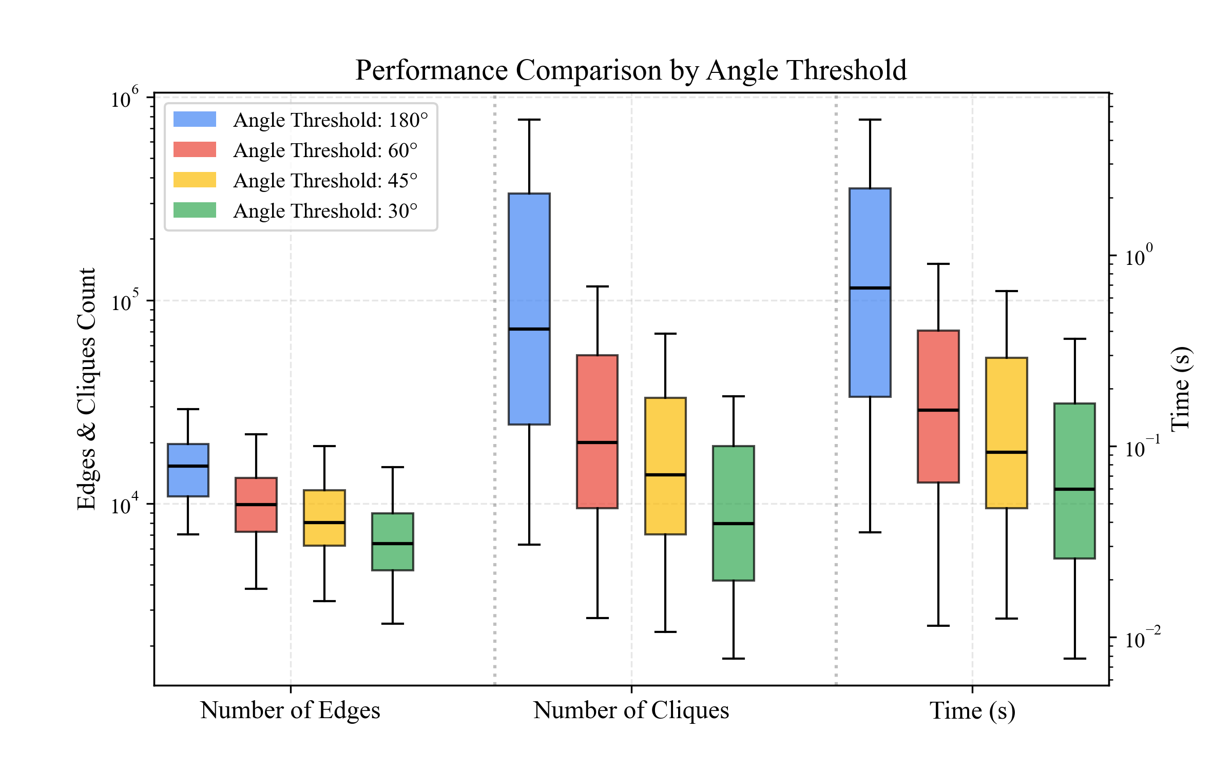
To validate the efficiency improvements achieved through normal-guided pruning, we adjust the normal consistency threshold $\delta_{\alpha}$ across four different values ranging from $180^{\circ}$ to $30^{\circ}$. For each threshold setting, we conduct 100 registration trials on the YCB-Reg dataset while maintaining identical front-end processing pipeline that consistently selected the same 500 correspondences to construct the consistency graph. As shown in Figure 9(a), tightening $\delta_{\alpha}$ consistently resulted in significant reductions in both edge density and the number of maximal cliques, leading to a pronounced decrease in computation time.

We further visualize the data distributions for $\delta_{\alpha}=180^{\circ}$ and $\delta_{\alpha}=30^{\circ}$ in Figure 9(b). Theoretically, maximal clique search has an exponential worst-case complexity of $O(3^{n/3})$ with respect to the number of graph nodes [31]. On the other hand, after applying normal-guided pruning, our results demonstrate an approximately polynomial relationship between the number of edges and computational cost. These findings indicate that normal-guided pruning effectively reduces the computational complexity of maximal clique search, thereby improving the efficiency of tactile localization.

V-E Computational Efficiency Analysis

We conduct a detailed per-stage computational profile to analyze the computational efficiency of TacLoc. All timing experiments were performed under CPU-serialized conditions on a portable computing device equipped with an Intel processor and 32GB of RAM. Figure 11 provides a statistical breakdown of time consumption across the different stages of TacLoc, revealing that FPFH-based initial correspondence and transformation verification are the most time-intensive stages.

In addition, we evaluate the efficiency and effectiveness of the method under varying $\delta_{d}$ and $\delta_{\alpha}$ in the consistency check. Theoretically, larger threshold values result in denser graph constructions, leading to longer computation times, while an increased number of incorrect correspondences introduces larger estimation errors. This analysis aligns with the conclusions drawn from Figure 10.

(a) $\delta_{d}$

(b) $\delta_{\alpha}$

Figure 10: Rotation error and time cost with varying thresholds $\delta_{d}$ and $\delta_{\alpha}$.

Figure 11: Per-stage computational profile. FPFH-based initial data association and transformation verification are the most time-intensive stages.

Figure 12: (a) TacLoc is deployed on two real-world sensors beyond the DIGIT used in YCB simulation, despite these sensors having different characteristics. The right side shows the visual-tactile images obtained from the sensors. (b) Evaluation on five real-world objects using the GelSight Mini. We perform sliding touches on the objects 50 times, and the proposed TacLoc achieves a success rate of 33/50. Note that the red object is used for the single-touch demonstration shown in Figure 1. The right side displays the successful cases, where the yellow points represent the submaps.

V-F Evaluation on Real-world Objects

To validate the generalization beyond simulation, we conduct exploratory tests on household objects using the GelSight Mini sensor. As shown in Figure 12, we deploy TacLoc on a knife, spoon, fork, tangram, and phone case. ICP [5] or NormalFlow [13] is used to obtain end-effector poses (forward kinematics is optional if a robot arm is used). Obtaining ground truth for tactile localization in the real world is challenging, so we consider the method to achieve successful localization if it produces visually plausible registrations. The overall success rate is 33/50 for the sliding touches on these five objects. We observe a higher success rate when the contact regions contain sufficient geometric features, with particularly clear alignments on objects exhibiting distinctive curvatures.

One might ask how partial or incorrect CAD models impact performance. When touching missing or incorrect parts, deviations between the actual tactile sensing and the designed CAD models will lead to incorrect correspondences and localization failures. Therefore, accurate CAD models are critical for tactile pose estimation. On the other hand, the proposed TacLoc could achieve tactile localization, though manufacturing defects exist in Figure 12.

Until now, we have tested DIGIT [17] in simulation and GelSight [37] on real-world objects. Additionally, we explore deploying TacLoc using a new Daimon sensor (Figure 12). We carefully tune the sensing component (like the scale) to obtain point clouds and successfully deploy TacLoc to achieve global tactile localization. These sensors exhibit different resolution characteristics, confirming the fundamental compatibility of proposed method across various sensing technologies. Notably, we observe that varying noise profiles and spatial resolutions can influence correspondence density, suggesting that sensor-specific tuning could further enhance performance.

VI Conclusion

In this study, we design a normal-aided graph pruning-based point cloud registration method for global tactile localization. We analyze and evaluate the proposed method in both simulation and real-world experiments. We consider two promising directions for future work. First, the fusion of tactile data from multiple tactile measurements [36] could be explored to enhance the accuracy and robustness of pose estimation through collaborative perception. Second, investigating strategies for active tactile exploration [24] could enable robots to interact with specific object regions while refining pose estimation.

References

- [1] (2021) Spinnet: learning a general surface descriptor for 3d point cloud registration. In Proceedings of the IEEE/CVF conference on computer vision and pattern recognition, pp. 11753–11762. Cited by: §II-B, §V-A2.
- [2] (2024) 3d-bbs: global localization for 3d point cloud scan matching using branch-and-bound algorithm. In 2024 IEEE International Conference on Robotics and Automation (ICRA), pp. 1796–1802. Cited by: §II-B.
- [3] (2023) Tac2pose: tactile object pose estimation from the first touch. The International Journal of Robotics Research 42 (13), pp. 1185–1209. Cited by: §I, §II-A, §II-A, §III.
- [4] (2019) Tactile mapping and localization from high-resolution tactile imprints. In 2019 International Conference on Robotics and Automation (ICRA), pp. 3811–3817. Cited by: §II-A.
- [5] (1992) Method for registration of 3-d shapes. In Sensor fusion IV: control paradigms and data structures, Vol. 1611, pp. 586–606. Cited by: §V-F.
- [6] (1973) Algorithm 457: finding all cliques of an undirected graph. Communications of the ACM 16 (9), pp. 575–577. Cited by: §IV-B2.
- [7] (2017) Yale-cmu-berkeley dataset for robotic manipulation research. The International Journal of Robotics Research 36 (3), pp. 261–268. Cited by: Figure 5, §V-A1.
- [8] (2024) Tactile-augmented radiance fields. In Proceedings of the IEEE/CVF Conference on Computer Vision and Pattern Recognition, pp. 26529–26539. Cited by: §III.
- [9] (2017) Segmatch: segment based place recognition in 3d point clouds. In 2017 IEEE international conference on robotics and automation (ICRA), pp. 5266–5272. Cited by: §I.
- [10] (2019) Rotation averaging with the chordal distance: global minimizers and strong duality. IEEE Transactions on Pattern Analysis and Machine Intelligence 43 (1), pp. 256–268. Cited by: §IV-B3.
- [11] (1981) Random sample consensus: a paradigm for model fitting with applications to image analysis and automated cartography. Communications of the ACM 24 (6), pp. 381–395. Cited by: §II-B, §V-A2.
- [12] (2008) Exploring network structure, dynamics, and function using networkx. Technical report Los Alamos National Laboratory (LANL), Los Alamos, NM (United States). Cited by: §IV-B2.
- [13] (2024) NormalFlow: fast, robust, and accurate contact-based object 6dof pose tracking with vision-based tactile sensors. IEEE Robotics and Automation Letters. Cited by: §V-F.
- [14] (1978) A discussion of the solution for the best rotation to relate two sets of vectors. Foundations of Crystallography 34 (5), pp. 827–828. Cited by: §IV-B3.
- [15] (2021) Minkloc3d: point cloud based large-scale place recognition. In Proceedings of the IEEE/CVF winter conference on applications of computer vision, pp. 1790–1799. Cited by: §II-A.
- [16] (2016) Deeper depth prediction with fully convolutional residual networks. In 2016 Fourth international conference on 3D vision (3DV), pp. 239–248. Cited by: §IV-A.
- [17] (2020) Digit: a novel design for a low-cost compact high-resolution tactile sensor with application to in-hand manipulation. IEEE Robotics and Automation Letters 5 (3), pp. 3838–3845. Cited by: §II-A, §IV-A, §V-A1, §V-F.
- [18] (2025) ViTaSCOPE: Visuo-tactile Implicit Representation for In-hand Pose and Extrinsic Contact Estimation. In Robotics: Science and Systems 2025, (en). Cited by: §II-A.
- [19] (2023) Vihope: visuotactile in-hand object 6d pose estimation with shape completion. IEEE Robotics and Automation Letters 8 (11), pp. 6963–6970. Cited by: §II-A.
- [20] (2014) Localization and manipulation of small parts using gelsight tactile sensing. In 2014 IEEE/RSJ International Conference on Intelligent Robots and Systems, pp. 3988–3993. Cited by: §II-A.
- [21] (2018) Efficient global point cloud registration by matching rotation invariant features through translation search. In Proceedings of the European Conference on Computer Vision (ECCV), pp. 448–463. Cited by: §IV-B3.
- [22] (2021) Clipper: a graph-theoretic framework for robust data association. In 2021 IEEE International Conference on Robotics and Automation (ICRA), pp. 13828–13834. Cited by: §II-B, §II-B.
- [23] (2024) TripletLoc: one-shot global localization using semantic triplet in urban environments. IEEE Robotics and Automation Letters. Cited by: §I.
- [24] (2023) Tactile-filter: interactive tactile perception for part mating. arXiv preprint arXiv:2303.06034. Cited by: §II-A, §VI.
- [25] (2011) Global localization of objects via touch. IEEE Transactions on Robotics 27 (3), pp. 569–585. Cited by: §I, §II-A, §III.
- [26] (2011) Object mapping, recognition, and localization from tactile geometry. In 2011 IEEE International Conference on Robotics and Automation, pp. 5942–5948. Cited by: §II-A.
- [27] (2021) Distinctive 3d local deep descriptors. In 2020 25th International conference on pattern recognition (ICPR), pp. 5720–5727. Cited by: §II-B, §V-A2.
- [28] (2024) G3reg: pyramid graph-based global registration using gaussian ellipsoid model. IEEE Transactions on Automation Science and Engineering 22, pp. 3416–3432. Cited by: §II-B, §II-B, §IV-B2.
- [29] (2009) Fast point feature histograms (fpfh) for 3d registration. In 2009 IEEE international conference on robotics and automation, pp. 3212–3217. Cited by: §II-B, §IV-A.
- [30] (2023) Midastouch: monte-carlo inference over distributions across sliding touch. In Conference on Robot Learning, pp. 319–331. Cited by: §I, §II-A, §II-A, §III, §V-A1, §V-C.
- [31] (2006) The worst-case time complexity for generating all maximal cliques and computational experiments. Theoretical computer science 363 (1), pp. 28–42. Cited by: §V-D.
- [32] (2022) Tacto: a fast, flexible, and open-source simulator for high-resolution vision-based tactile sensors. IEEE Robotics and Automation Letters 7 (2), pp. 3930–3937. Cited by: §V-A1.
- [33] (2020) Teaser: fast and certifiable point cloud registration. IEEE Transactions on Robotics 37 (2), pp. 314–333. Cited by: §V-A2.
- [34] (2024) Mac: maximal cliques for 3d registration. IEEE Transactions on Pattern Analysis and Machine Intelligence. Cited by: §II-B, §II-B, §IV-B2, §V-A2.
- [35] (2024) A survey on global lidar localization: challenges, advances and open problems. International Journal of Computer Vision 132 (8), pp. 3139–3171. Cited by: §I, §II-B, §III.
- [36] (2025) Multi-tactile sensor calibration via motion constraints with tactile measurements. The International Journal of Robotics Research 44 (7), pp. 1217–1230. Cited by: §VI.
- [37] (2017) Gelsight: high-resolution robot tactile sensors for estimating geometry and force. Sensors 17 (12), pp. 2762. Cited by: §II-A, §II-A, §IV-A, §V-F.
- [38] (2009) Intrinsic shape signatures: a shape descriptor for 3d object recognition. In 2009 IEEE 12th international conference on computer vision workshops, ICCV Workshops, pp. 689–696. Cited by: §IV-A.