One Token, Two Fates: A Unified Framework via Vision Token Manipulation Against MLLMs Hallucination

Abstract

Current training-free methods tackle MLLM hallucination with separate strategies: either enhancing visual signals or suppressing text inertia. However, these separate methods are insufficient due to critical trade-offs: simply enhancing vision often fails against strong language prior, while suppressing language can introduce extra image-irrelevant noise. Moreover, we find their naive combination is also ineffective, necessitating a unified framework. We propose such a framework by focusing on the core asset: the vision token. Our design leverages two key insights: (1) augmented images offer complementary visual semantics, and (2) removing vision tokens (information-gap) isolates hallucination tendencies more precisely than distorting images (modality-gap). Based on these, our framework uses vision tokens in two distinct ways, both operating on latent representations: our Synergistic Visual Calibration (SVC) module incorporates augmented tokens to strengthen visual representations, while our Causal Representation Calibration (CRC) module uses pruned tokens to create latent-space negative samples for correcting internal model biases. By harmonizing these two roles, our framework effectively restores the vision-language balance, significantly reducing object hallucinations, improving POPE accuracy by an average of 2% absolute on LLaVA-1.5 across multiple benchmarks with only a 1.06x inference latency overhead.

1 Introduction

Figure 1: Disjoint Paradigms vs. Our Unified Latent Calibration. (a) Prior work includes Visual Attention Enhancement [27] and (b) Textual Decoding Refinement at final logits [20]. Naively combining these disjoint paradigms (a)+(b) degrades performance, highlighting conflicting signals. (c) Our Unified Latent Calibration is a unified system operating entirely at the representation level, using the vision token as a single source for both SVC and CRC, achieving superior and synergistic results.

Figure 2: Our Three Core Findings. (F1) Diagnosing the Imbalance: Inverse Correlation. Visual attention decays sharply as generation proceeds, while hallucination frequency surges where visual grounding is weakest. (F2) Enabling Enhancement: Semantic Complementarity. Original and augmented image attentions show complementary focus (e.g., on ’Camera’); their synergy enables enhanced visual grounding. (F3) Enabling Calibration: Superiority of Information-Gap. Latent-space token removal (information-gap) generates stable, grounded hallucinations, proving more suitable for bias probing than unstable, noisy pixel-level masking (modality-gap).

Multimodal learning, Large Language Models (LLMs) and Multimodal Large Language Models (MLLMs) represent significant progress in artificial intelligence, showing powerful capabilities in understanding and reasoning about the world [26, 2, 46, 9, 6, 3]. The vision token is the key bridge connecting image signals and text signals in these models, making it a central focus of study [29, 12, 40]. However, the reliability of MLLMs is undermined by a critical flaw: hallucination [25, 20, 15], which refers to the fact that MLLMs generate fluent text that contradicts the visual evidence, posing a major barrier to realistic use.

At its core, as commonly discussed in prior works [27, 31, 33], MLLM hallucination stems from a fundamental imbalance: the visual signal progressively weakens during outputting, while the model’s strong internal language prior takes over. Our analysis confirms this imbalance (Figure 2(F1)), showing that visual attention decays sharply as text generation, precisely when hallucinations are most likely to appear, posing a core problem: visual signals gradually weaken over time compared to language signals.

Existing training-free strategies try to fix this imbalance using disjoint approaches, as depicted in Figure 1. Some focus on Visual Attention Enhancement (Fig. 1(a)) by boosting attention weights to amplify the visual signal [27, 41, 36]. Others apply Textual Decoding Refinement (Fig. 1(b)), using negative samples for contrastive decoding at the final output logits to suppress text inertia [20, 43, 44, 11]. But why is unification necessary? We contend these separate methods face a critical trade-off:

• Why enhancing vision alone falls short: Simply boosting the visual signal (e.g., strengthening attention) often isn’t enough to ensure accuracy. The language model component has strong ingrained tendencies (text inertia) [23] that can still dominate the text generation, especially as the influence of the image naturally weakens over longer outputs (F1). As confirmed by prior studies [18, 20], this language inertia is a persistent and inevitable challenge.

• Why suppressing language alone has drawbacks: Methods focusing only on correcting the language model’s text inertia often rely on creating negative examples by distorting the input image (modality-gap) [20, 5]. Our analysis (F3) shows these distorted images create unreliable contents, results are unstable and unrelated to the visual detail, bringing extra noise. Relying on noisy signals for correction means the answers can become unpredictable.

Therefore, MLLM hallucination reflects a systemic imbalance requiring a holistic solution.

However, designing such a unified framework is a non-trivial challenge. A simple, “patchwork” combination of these disjoint methods is not a principled solution. As we empirically demonstrate in Figure 1, naively combining an attention enhancement method (PAI [27]) with a decoding refinement method (VCD [20]) actually performs no improvement. This happens because the two methods aren’t designed to work together. One boosts visual details from the original image at the attention stage, while the other suppresses signals at the logit level using a negative sample. Furthermore, their calibration timings are different: one intervenes during the layer-level processing, while the other applies a post-correction at the final output stage.

So How to achieve true, synergistic unification? Recognizing this obstacle, we argue a framework must operate cohesively at the same level. We turned our focus towards the nexus of the vision-language interaction: the vision token. Could manipulating this core asset directly offer a path to a unified latent representation calibration?

By systematically investigating the vision token’s potential, we uncovered other two foundational Findings (Figure 2) that reveal the key mechanisms for restoring balance and directly enable our unified design:

• (F2) Semantic Complementarity: We discovered that augmented vision tokens offer complementary semantics, providing a crucial base to build a richer visual anchor for enhancement, as similarly explored in [14, 8, 40].

• (F3) Information-Gap for Negative Sampling: We demonstrated that an information-gap (by removing tokens in latent space) yields a superior, in-distribution probe for isolating bias, compared to noisy modality-gap based image-level-distorting methods.

These findings reveal that the vision token possesses the potential to serve two distinct roles simultaneously, which corresponds to two fates. Based on this, we propose the first unified, training-free framework that operates at the intermediate representation level (Figure 1(c)). It derives all calibration signals from the vision token:

• For enhancement, our Synergistic Visual Calibration (SVC) module (based on F2) uses augmented tokens to inject a comprehensive visual context, counteracting visual fading (F1).

• For suppression, our Causal Representation Calibration (CRC) module (based on F3) uses pruned tokens to craft “latent-space negative samples” for precisely purifying model internal biases.

By addressing both sides of the vision-language imbalance through this principled manipulation of vision tokens, our contributions can be summarized as:

1. We reframe hallucination mitigation as a vision-language balance problem, highlighting the limitations of disjointed approaches and demonstrating the failure of naive combination. This reframing is grounded in our systematic analysis of vision tokens, which reveals their dual potential for both enhancement and calibration.

2. We propose the first unified latent calibration framework that harmonizes enhancement and suppression by leveraging the dual potential of vision tokens, operating entirely on intermediate representations.

3. We introduce SVC and CRC as novel, efficient modules instantiating this unified method for targeted enhancement and precise suppression.

Our framework demonstrates superior performance and efficiency across diverse benchmarks, validating our unified, vision-token-centric approach.

2 Methodology

This section details our proposed unified framework for mitigating MLLM hallucinations by restoring the vision-language balance. We first establish the necessary notation in Sec. 2.1. Then, we present the overall architecture of our unified framework in Sec. 2.2. Finally, we elaborate on the two core modules: the Synergistic Visual Calibration (SVC) module in Sec. 2.3, which leverages semantic complementarity (F2) to counteract visual fading (F1), and the Causal Representation Calibration (CRC) module in Sec. 2.4, which employs the information-gap principle (F3) for precise bias suppression.

Figure 3: Overview of our unified framework. The model processes an original input stream (orange path) and a parallel hallucination-probe stream (purple path) derived from pruned vision tokens. Our Synergistic Visual Calibration (SVC) module injects complementary visual context from augmented images into a critical middle layer ($L_{c}$) to counteract visual fading. Simultaneously, the Causal Representation Calibration (CRC) module uses the differential representations between the two streams to purify hidden states in shallow layers ($1\dots L_{c}$), suppressing linguistic priors.

Figure 4: Illustration of the Causal Representation Calibration (CRC) mechanism. By subtracting the hallucinated representation ($\mathbf{H}_{\text{neg}}$) from the original ($\mathbf{H}_{\text{org}}$), we obtain a differential vector ($\Delta\mathbf{H}$). Averaging these vectors across multiple negative samples yields a stable hallucination direction ($\mathbf{v}_{\text{crc}}$). The final calibration modifies the original representation away from this direction to produce a purified output ($\mathbf{H}_{\text{pos}}$).

2.1 Preliminaries

We consider a standard MLLM parameterized by $\theta$ that autoregressively generates a response $\mathbf{y}=\{y_{1},\ldots,y_{L_{y}}\}$ given an image $I$ and query $T$. The image is encoded into vision tokens $\mathbf{V}\in\mathbb{R}^{N_{v}\times d}$, and the query into text tokens $\mathbf{Q}\in\mathbb{R}^{N_{q}\times d}$. These form the initial context $\mathbf{X}_{\text{context}}=[\mathbf{V};\mathbf{Q}]$ for the $L$-layer Transformer decoder $\mathcal{D}$.

At generation step $t$, the decoder processes the input embeddings $\mathbf{H}_{t}^{(0)}$ (derived from $\mathbf{X}_{\text{context}}$ and previous tokens $\mathbf{y}_{<t}$) layer by layer. The output hidden states from any intermediate layer $l\in[1,L]$ are denoted as:

$$\mathbf{H}_{t}^{(l)}=\mathcal{D}^{(1\dots l)}(\mathbf{H}_{t}^{(0)}),$$ (1)

which are crucial for our intervention modules. The probability distribution for the next token $y_{t}$ is obtained via a softmax over the logits function $f_{\theta}$:

$$y_{t}\sim p_{\theta}(y_{t}|I,T,\mathbf{y}_{<t})=\text{softmax}(f_{\theta}(I,T,\mathbf{y}_{<t})).$$ (2)

This proceeds iteratively until meeting stopping criterion.

2.2 Overview

Our unified, training-free framework (Figure 3) restores the vision-language balance by repurposing vision tokens for two complementary roles. To address visual fading, our Synergistic Visual Calibration (SVC) module injects an enriched visual context (from original and augmented images) into a critical middle layer via attention. To counteract text inertia, our Causal Representation Calibration (CRC) module intervenes in shallow layers. It crafts latent-level negative samples via token pruning to distill a stable hallucination direction vector, which is then subtracted from the main computational stream to purify the hidden states. For efficiency, SVC intervenes at a single layer (e.g., layer 16 [39, 19, 4]), while CRC applies its calibration from the initial layers up to targeted layer. All operations are performed directly on the intermediate representation, bypassing decoding, thereby maximizing inference efficiency.

2.3 Synergistic Visual Calibration (SVC)

To counteract the visual fading phenomenon (F1), we introduce the SVC module, motivated by our finding on semantic complementarity (F2) and prior works [40, 14, 8, 47].

Synergistic Visual Context Construction.

Given an image $I$, we create an augmented version $I_{\text{aug}}$ by applying random horizontal flipping, Gaussian blur with radius 5, and salt-and-pepper noise (intensity = 0.2). Both are processed to obtain their vision token, $\mathbf{V},\mathbf{V}_{\text{aug}}\in\mathbb{R}^{N_{v}\times d}$. We concatenate them to form a synergistic visual memory bank:

$$\mathbf{V}_{\text{syn}}=[\mathbf{V};\mathbf{V}_{\text{aug}}]\in\mathbb{R}^{2N_{v}\times d}.$$ (3)

Parameter-Free Visual Injection.

SVC intervenes at a single, pre-defined middle layer $L_{c}$. At generation step $t$, we intercept the hidden state sequence $\mathbf{H}_{t}^{(L_{c}-1)}$ from the preceding layer, which serves as the Query. The set $\mathbf{V}_{\text{syn}}$ serves as both Key and Value. A visual context sequence $\mathbf{C}_{t}$ is computed via scaled dot-product attention:

$$\mathbf{C}_{t}=\text{softmax}\left(\frac{\mathbf{H}_{t}^{(L_{c}-1)}(\mathbf{V}_{\text{syn}})^{T}}{\sqrt{d}}\right)\mathbf{V}_{\text{syn}}.$$ (4)

As implemented, the resulting context $\mathbf{C}_{t}$ is integrated via interpolation, blending it with the original hidden state:

$$\mathbf{H}^{\prime(L_{c})}_{t}=(1-\lambda_{s})\cdot\mathbf{H}^{(L_{c})}_{t}+\lambda_{s}\cdot\mathbf{C}_{t},$$ (5)

where $\lambda_{s}$ is a hyperparameter controlling the interpolation ratio. This updated hidden state $\mathbf{H}^{\prime(L_{c})}_{t}$ proceeds to the next layer, re-engaging the model with a richer visual context.

2.4 Causal Representation Calibration (CRC)

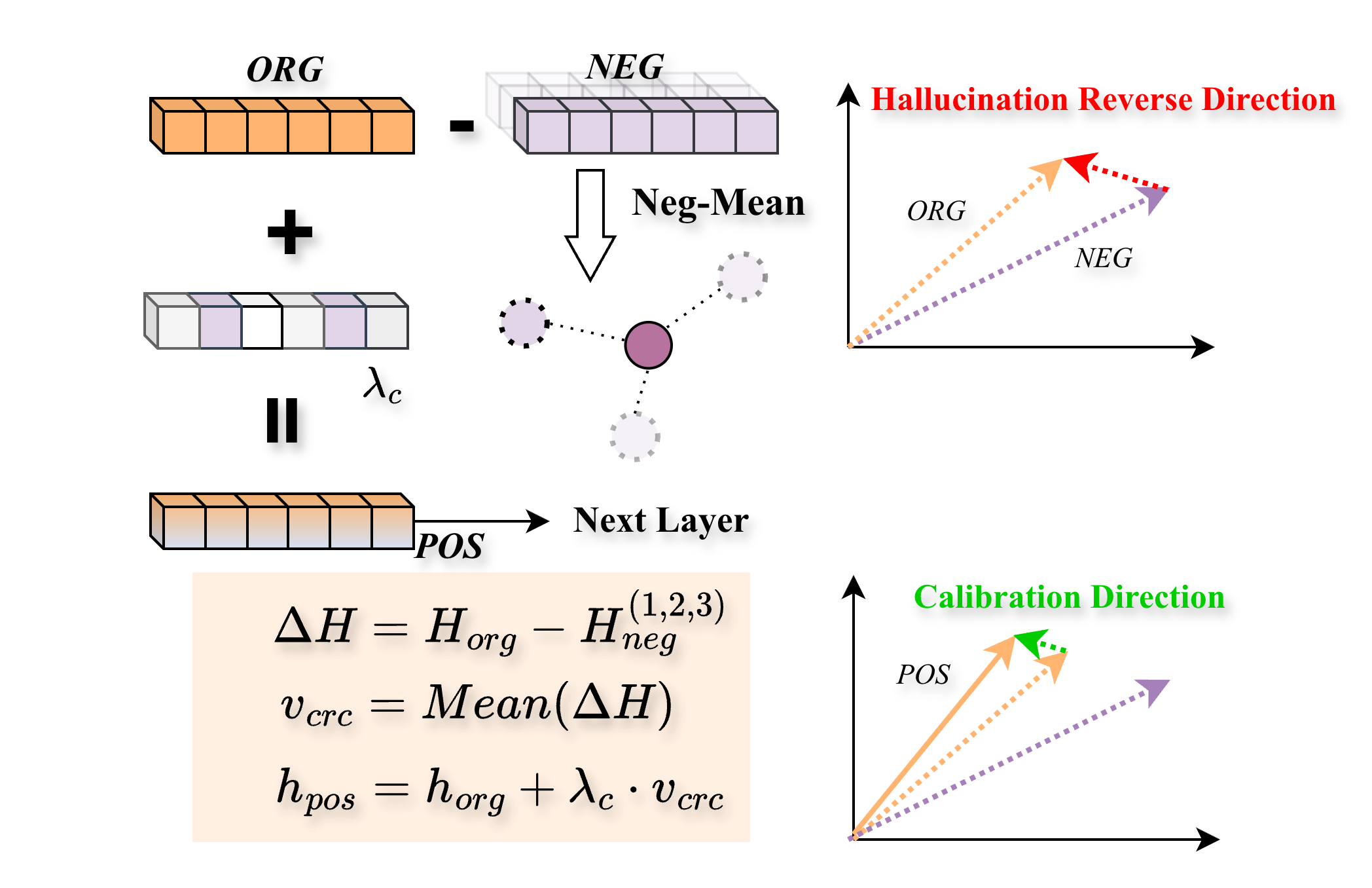
Distinct from prior methods operating on output logits, CRC intervenes on intermediate representations to neutralize the “hallucination direction”, visualized in Figure 4.

Probing for the Hallucination Direction.

To isolate intrinsic biases, We craft “latent space negative samples” based on our information-gap principle (F3). Given the original vision token sequence $\mathbf{V}\in\mathbb{R}^{N_{v}\times d}$, we generate $K$ negative samples, $\{\mathbf{V}_{\text{neg}}^{(k)}\}_{k=1}^{K}$, by randomly pruning $\mathbf{V}$ to retain only $N_{h}=5$ tokens.

At the first step $t=0$, we run parallel forward passes through the layers for the original and negative samples:

$$\mathbf{H}_{0,\text{org}}^{(l)} =\mathcal{D}^{(1\dots l)}(\,[\mathbf{V};\mathbf{Q}]\,),$$ (6)

$$\mathbf{H}_{0,\text{neg}}^{(l,k)} =\mathcal{D}^{(1\dots l)}(\,[\mathbf{V}_{\text{neg}}^{(k)};\mathbf{Q}]\,).$$ (7)

The difference, $\Delta\mathbf{H}^{(l,k)}=\mathbf{H}_{0,\text{org}}^{(l)}-\mathbf{H}_{0,\text{neg}}^{(l,k)}$, captures the representational shift. We compute the stable hallucination vector $\mathbf{v}_{\text{crc}}^{(l)}$ by averaging this difference:

$$\mathbf{v}_{\text{crc}}^{(l)}=\frac{1}{K}\sum_{k=1}^{K}\Delta\mathbf{H}^{(l,k)}.$$ (8)

This vector $\mathbf{v}_{\text{crc}}^{(l)}$ acts as our representation probe cache and is re-used for all subsequent processing steps.

Causal Calibration.

At each generation step $t>0$, we perform calibration by adjusting the current hidden state. This operation is performed in normalized space to preserve representation stability. First, the original state and the calibration vector are normalized:

$$\mathbf{h}_{\text{norm}}=\frac{\mathbf{H}_{t,\text{org}}^{(l)}}{||\mathbf{H}_{t,\text{org}}^{(l)}||_{2}},\quad\mathbf{v}_{\text{norm}}=\frac{\mathbf{v}_{\text{crc}}^{(l)}}{||\mathbf{v}_{\text{crc}}^{(l)}||_{2}}.$$ (9)

Next, a new unnormalized vector $\mathbf{h}_{\text{crc}}$ is computed by linearly combining the normalized vectors:

$$\mathbf{h}_{\text{crc}}=\mathbf{h}_{\text{norm}}+\lambda_{c}\cdot\mathbf{v}_{\text{norm}}.$$ (10)

Finally, the corrected hidden state $\mathbf{H}_{t,\text{pos}}^{(l)}$ is obtained by re-normalizing this vector and scaling it back to the original magnitude of $\mathbf{H}_{t,\text{org}}^{(l)}$:

$$\mathbf{H}_{t,\text{pos}}^{(l)}=\frac{\mathbf{h}_{\text{crc}}}{||\mathbf{h}_{\text{crc}}||_{2}}\cdot||\mathbf{H}_{t,\text{org}}^{(l)}||_{2},$$ (11)

where $\lambda_{c}$ is a hyperparameter. This calibrated representation proceeds to the next layer. This process is repeated for all layers $l=1,\dots,L_{c}$.

Figure 5: The simplified Structural Causal Model (SCM) for MLLM hallucination. We posit that hallucination arises from a spurious causal path from the model’s intrinsic bias ($B$) to its latent representation ($H^{(l)}$), which confounds the true visual path from the image ($V$).

Theoretical Justification.

Our Causal Representation Calibration (CRC) is grounded in Structural Causal Models (SCM). We model hallucination (Figure 5) as arising from a spurious causal path where intrinsic bias ($B$) confounds the true visual path ($V\to H_{t}^{(l)}$). This bias includes inherent noise and linguistic priors. Our essential negative sample, derived from a degraded visual input $V_{\text{neg}}$, acts as an in-distribution causal probe by retaining the original image’s structural properties.

The core theoretical insight is that our differential vector $\mathbf{v}_{\text{crc}}$ isolates the causal effect of the missing visual information. Following a commonly adopted local linear approximation supported by [16, 30, 13, 45], we estimate the hidden states decompose as:

$$\mathbf{H}_{t,\text{org}}^{(l)} \approx\mathcal{E}(V)+\mathcal{E}_{\text{shared}}(Q,B)$$ (12)

$$\mathbf{H}_{t,\text{neg}}^{(l)} \approx\mathcal{E}(V_{\text{neg}})+\mathcal{E}_{\text{shared}}(Q,B)$$ (13)

where $\mathcal{E}(\cdot)$ is the causal effect function. Subtracting these cancels the shared query ($Q$) and bias ($B$) effects. Thus, our representation probe captures the pure visual difference:

$$\mathbf{v}_{\text{crc}}^{(l)}\approx\mathcal{E}(V-V_{\text{neg}}),$$ (14)

which represents the pure signal lost due to degradation. The calibration step Eq.(10) uses this to perform a counterfactual adjustment, towards visual truth representation.

Summary.  Eq.(14) provides a principled way to estimate the pure visual signal to cancel shared effects of the text prior and internal bias.

3 Experiments

Benchmark	Method	LLaVA-1.5		MiniGPT-4		Shikra		InstructBLIP
		Avg. Accuracy $\uparrow$	Avg. F1 $\uparrow$	Avg. Accuracy $\uparrow$	Avg. F1 $\uparrow$	Avg. Accuracy $\uparrow$	Avg. F1 $\uparrow$	Avg. Accuracy $\uparrow$	Avg. F1 $\uparrow$
MSCOCO	Vanilla	84.79	85.61	76.76	76.82	81.32	82.01	84.36	84.64
	VCD [CVPR’24]	84.80	85.65	76.01	76.28	81.34	82.25	84.81	85.28
	PAI [ECCV’24]	85.85	86.08	75.64	77.57	81.30	80.81	83.98	84.02
	VISTA [ICML’25]	86.15	86.29	76.06	76.80	82.44	82.47	84.87	84.95
	ONLY [ICCV’25]	86.03	86.22	76.98	77.62	82.75	82.85	84.90	85.01
highlightcolor	Ours	86.79	87.04	76.78	77.29	83.84	83.58	84.59	84.97
AOKVQA	Vanilla	77.23	80.62	72.80	72.99	78.67	80.03	78.92	81.51
	VCD [CVPR’24]	76.29	79.99	71.27	71.93	78.52	80.24	78.95	81.52
	PAI [ECCV’24]	78.65	79.82	73.20	73.22	79.97	81.07	79.04	81.77
	VISTA [ICML’25]	81.23	81.65	71.82	72.34	80.12	81.24	80.09	82.30
	ONLY [ICCV’25]	80.55	82.24	72.54	72.56	81.64	81.78	80.76	82.58
highlightcolor	Ours	82.23	83.82	73.13	73.69	81.87	82.18	80.24	82.48
GQA	Vanilla	78.76	80.79	70.81	73.08	78.59	79.70	77.31	79.08
	VCD [CVPR’24]	79.36	80.92	70.60	72.98	78.89	79.96	77.11	78.98
	PAI [ECCV’24]	79.80	81.12	71.12	73.20	79.23	80.16	77.56	79.18
	VISTA [ICML’25]	80.89	82.37	71.13	73.19	79.59	80.20	78.01	80.34
	ONLY [ICCV’25]	80.44	82.17	71.99	73.89	80.28	81.02	77.98	80.32
highlightcolor	Ours	81.54	83.38	71.40	73.37	81.24	81.44	78.11	80.29

Table 1: Evaluation results on POPE benchmark across four MLLMs. Results show averaged accuracy and F1 scores in % computed across random, popular, and adversarial object splits. Best and second best results are bolded and underlined, respectively.

Max Tokens	Method	LLaVA-1.5		MiniGPT-4		Shikra		InstructBLIP
		$\text{CHAIR}_{\text{Sen}}\downarrow$	$\text{CHAIR}_{\text{Ins}}\downarrow$	$\text{CHAIR}_{\text{Sen}}\downarrow$	$\text{CHAIR}_{\text{Ins}}\downarrow$	$\text{CHAIR}_{\text{Sen}}\downarrow$	$\text{CHAIR}_{\text{Ins}}\downarrow$	$\text{CHAIR}_{\text{Sen}}\downarrow$	$\text{CHAIR}_{\text{Ins}}\downarrow$
64 tokens	Vanilla	25.4	8.9	25.0	9.4	25.4	8.8	26.8	9.2
	VCD [CVPR’24]	24.1	7.9	25.4	9.4	23.2	8.1	26.8	9.3
	VISTA [ICML’25]	21.4	8.1	22.2	8.2	19.5	6.7	24.4	8.8
	ONLY [ICCV’25]	19.2	7.5	24.5	9.3	21.4	7.5	25.7	9.0
highlightcolor	Ours	18.1	8.4	23.8	8.3	16.7	5.9	24.2	7.9
128 tokens	Vanilla	48.9	14.9	36.4	11.3	56.8	15.6	43.2	12.4
	VCD [CVPR’24]	47.4	12.9	35.4	10.8	49.4	13.4	42.1	12.3
	VISTA [ICML’25]	38.6	11.7	31.2	10.2	36.4	10.8	36.2	10.4
	ONLY [ICCV’25]	42.2	12.4	33.9	10.6	38.2	11.4	40.2	11.6
highlightcolor	Ours	36.8	11.7	30.6	9.9	33.4	9.9	39.4	11.5

Table 2: CHAIR hallucination evaluation results. We compare our method to state-of-the-art training-free methods. Maximum new token is set to 64 and 128. Best and second best results are bolded and underlined, respectively.

Figure 6:   MMHal-Bench Evaluation across four MLLMs. Our method (Ours, orange line) consistently achieves superior performance across all eight categories, demonstrated by the larger area covered in the radar plots compared to Vanilla, PAI, and VISTA.  

In this section, we validate our framework across multiple MLLM architectures and four popular benchmarks. We first present the experimental configuration (Sec. 3.1), followed by an extensive evaluation on hallucination (Sec. 3.2) and general comprehensive benchmarks (Sec. 3.3), and finally we quantify the computational cost (Sec. 3.4).

3.1 Experimental Setup

Model Architectures.

We mainly evaluate our unified framework on four representative MLLMs with distinct architectural designs include: LLaVA-1.5 [26] and Shikra [6], which employ linear projections for visual-textual alignment, and MiniGPT-4 [46] and InstructBLIP [9], which utilize a Q-Former for cross-modal interaction.

Implementation Details.

We employ the following configuration across all experiments unless stated otherwise. For our Synergistic Visual Calibration (SVC) module, the intervention layer is set to $L_{c}=16$ for all models, and the scaling factor $\lambda_{s}$ is set to 0.06. For our Causal Representation Calibration (CRC) module, the pruning retains $N_{h}=5$ vision tokens, the number of negative samples is $K=3$ for balance of effectiveness and efficiency, and the calibration strength $\lambda_{c}$ is set to 0.1 by default.

3.2 Results on Object Hallucination Benchmarks

We first evaluate our framework on the two widely adopted benchmarks that assess object hallucination: POPE [22] and CHAIR [32]. We compare our method against several recent strong training-free based baselines, including VCD [20], PAI [27], VISTA [23], ONLY [37].

POPE Evaluation. The POPE benchmark [22] assesses object hallucination via yes/no questions (e.g., “Is there a [object] in the image?”) across three splits of increasing difficulty. As shown in Table 1, our method consistently outperforms prior work: on the challenging GQA split, it achieves 81.54% accuracy with LLaVA-1.5 and 78.11% with InstructBLIP, demonstrating strong generalizability across architectures (linear projector vs. Q-Former) and datasets (COCO [24], AOKVQA [34], GQA [17]).

CHAIR Evaluation. CHAIR [32] measures hallucinated objects in open-ended captions via instance-level ($\text{CHAIR}_{I}$) and sentence-level ($\text{CHAIR}_{S}$) scores (lower is better). Table 2 shows our approach achieves the best $\text{CHAIR}_{I}$ scores: 18.1 (LLaVA-1.5) and 16.7 (Shikra) at 64 tokens, and 30.6 (MiniGPT-4) and 33.4 (Shikra) at 128 tokens, confirming that our latent-level calibration effectively suppresses ungrounded object generation.

Method	LLaVA-1.5		InstructBlip
	$\text{Perception}_{\text{sum}}$	$\text{Cognition}_{\text{sum}}$	$\text{Perception}_{\text{sum}}$	$\text{Cognition}_{\text{sum}}$
Vanilla	1444.23	323.14	1181.15	233.71
VCD	1445.13	324.25	1182.34	234.95
VISTA	1450.54	329.08	1189.23	236.25
highlightcolor Ours	1456.28	332.86	1192.76	240.83

Table 3: Evaluation on MME benchmark (Perception and Cognition scores). Our method (Ours) consistently achieves state-of-the-art performance across all tested models, demonstrating robust general capabilities.

Method	Latency (ms/token)	Throughput (token/ms)	Memory Cost (MB)
Greedy	30.3 (×1.00)	0.033 (×1.00)	14257
ICD	33.03 (×1.09)	0.030 (×0.91)	14263
VCD	72.72 (×2.4)	0.014 (×0.42)	14984
VISTA	33.35 (×1.1)	0.030 (×0.91)	15024
highlightcolor Ours	32.1 (×1.06)	0.031 (×0.94)	14924

Table 4: Comparison of overhead among different methods (with best results bolded). Latency is measured in milliseconds per token. Throughput is calculated as tokens per millisecond. Memory cost is the peak GPU memory usage in megabytes.

3.3 Results on Comprehensive Benchmarks

A critical aspect of our framework is its ability to suppress hallucinations without harming the model’s general perception and reasoning abilities. We validate this on MMHal-Bench and MME.

MMHal-Bench Evaluation. MMHal-Bench [35] assesses hallucination via 96 image-question pairs across eight categories (e.g., colors, counting), focusing on complex visual reasoning. Responses are scored by GPT-4 [1]. As shown in Figure 6, our method outperforms Vanilla, PAI [27], and VISTA [23] across all categories on multiple MLLMs, with notable gains in ATTR, and ENV, indicating better use of true visual signals.

MME Evaluation. On MME [42], which evaluates 14 perception and cognition abilities, our framework improves general performance and hallucination mitigation. On LLaVA-1.5, we achieve Perception: 1456.28 and Cognition: 332.86, surpassing Vanilla, VCD, and VISTA; similar gains are seen on InstructBLIP (Perception: 1192.76, Cognition: 240.83). confirming our method enhances MLLM capabilities by better balancing vision and language.

3.4 Computational Overhead

Our framework is highly efficient, which is highly crucial for a training-free style method. As shown in Table 4, it incurs only a 1.06× latency increase over Greedy and faster than VISTA (33.35 ms/token) and VCD (72.72 ms/token). It also uses less peak GPU memory (14,924 MB) than VISTA (15,024 MB) and VCD (14,984 MB). Thus, this proves our method achieves strong hallucination mitigation with minimal computational overhead.

4 Discussions

We now analyze our framework’s components and design choices through ablation studies and visualizations. All discussions are based on experiments conducted on LLaVA-1.5 using POPE benchmarks unless otherwise specified.

4.1 Ablation Study

Method Configuration	COCO		AOKVQA
	Acc $\uparrow$	F1 $\uparrow$	Acc $\uparrow$	F1 $\uparrow$
Vanilla LLaVA-1.5	84.79	85.61	77.23	80.62
+ SVC ($V_{\text{ori}}$ only)	85.04	85.68	79.03	80.96
+ SVC ($V_{\text{syn}}$, Ours)	85.55	86.04	79.43	81.73
+ CRC (Masked Image neg.)	84.77	85.72	79.15	81.34
+ CRC (Pruned Token neg., Ours)	86.11	86.39	81.65	81.98
highlightcolor Ours (SVC + CRC)	86.79	87.04	82.23	83.82

Table 5: Ablation study on LLaVA-1.5 (POPE benchmark in %) evaluating our SVC variants (visual context) and CRC variants (negative sampling strategy). Best results are bolded.

Table 5 shows the results of our ablation study. Both our key modules, SVC (using $V_{\text{syn}}$) and CRC (using pruned tokens), improve performance individually over the Vanilla baseline. Notably, the full model integrating both SVC and CRC achieves the best scores across all metrics. This confirms that our two modules are effective and work synergistically, validating our unified design.

4.2 Why SVC works

Figure 7: Visualizing SVC’s effect with TAM [21]. For the token ’bulldog’, Vanilla LLaVA shows diffuse attention. $V_{\text{ori}}$ and $V_{\text{aug}}$ alone show different, complementary focus. ($+SVC(\text{Ours})$) integrates these cues, creating a accurate focus on the bulldog.

To understand SVC, we use Token Activation Mapping (TAM) [21] to visualize where the model attends (Figure 7). Focusing on the token ‘bulldog’ in a case with unchanged output, we find the Vanilla model exhibits diffuse attention. Using only the original ($V_{\text{ori}}$) or augmented ($V_{\text{aug}}$) image yields distinct, complementary attention patterns (F2). Our full SVC, which fuses both, produces a sharper, more focused map on the bulldog, demonstrating that our SVC leverages complementary visual cues to better ground attention on original image-relevant details.

4.3 Why CRC works

Figure 8: t-SNE visualization of hidden states. Our pruned-token negative samples (Our_Neg1/2/3) consistently cluster near the original (Ori_IMG) representations, suggesting an in-distribution probe. In contrast, Masked_IMG representations are divergent, indicating a noisy, out-of-distribution perturbation.

CRC’s effectiveness relies on our information-gap principle (F3): latent-space pruning is a better negative sampling strategy than pixel-level masking. We verify this using t-SNE visualizations [28] of hidden states (Figure 8). Across all four MLLMs, a clear pattern emerges: our pruned-token negative samples (Our_Neg1/2/3) produce representations that cluster close to the original image’s representations (Ori_IMG). This suggests our method is an in-distribution probe. In contrast, masked image (Masked_IMG) representations are often in completely different, distant clusters, suggesting a noisy, out-of-distribution perturbation. This indicates that our CRC method uses a cleaner, more relevant signal to isolate bias, enabling a more precise calibration.

4.4 Analysis over Hyperparameters

Figure 9: Hyperparameter Analysis. (a) POPE Accuracy vs. Latency for different $K$ in CRC. We choose $K=3$ (red star) as the best balance of performance and speed. (b) Heatmap for SVC ($\lambda_{s}$) and CRC ($\lambda_{c}$) strength. Performance is robust, with an optimal region around $\lambda_{s}=0.06$ and $\lambda_{c}=0.10$.

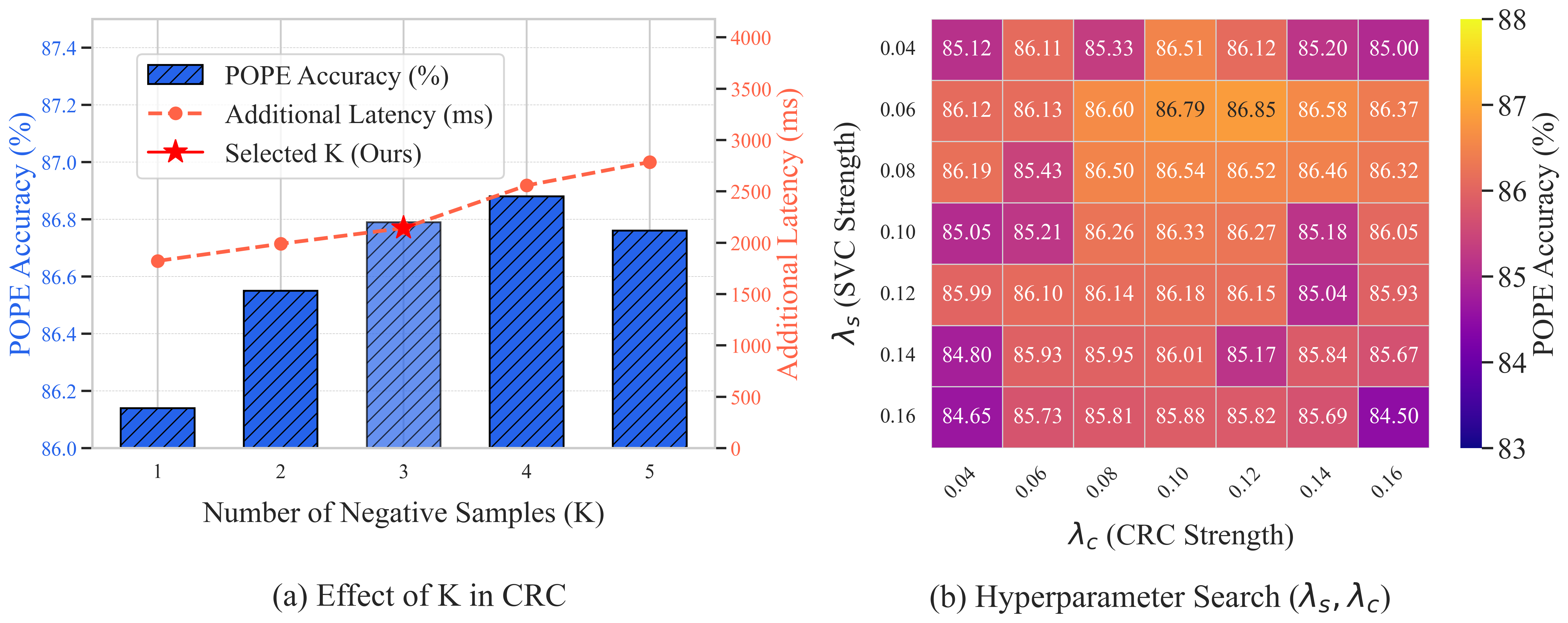
Choice of K. $K$ impacts both accuracy and speed. As shown in Figure 9(a), performance peaks at $K=3$. While more samples add some stability, they also add extra latency. We thus select $K=3$ as the best trade-off.

Calibration Strengths $\lambda_{s}$ and $\lambda_{c}$. The heatmap in Figure 9(b) shows our grid search results. Performance is stable across a wide range of values, confirming our method is not overly sensitive to these hyperparameters. We selected $\lambda_{s}=0.06$ and $\lambda_{c}=0.10$ as our default, as this region provides relatively strong results.

Choice of $N_{h}$. Unlike model pruning to accelerate decoding speed [7, 10, 38], our goal is to reduce visual grounding to induce a measurable hallucination signal. Our study (Figure 10) shows LLaVA-1.5’s POPE accuracy is remarkably robust to random pruning, remaining stable even at $N_{h}=50$ (from 576). A noticeable decline begins only below $N_{h}=20$, with a sharp drop at $N_{h}=5$. This confirms $N_{h}\geq 20$ provides too much visual information, failing to trigger the bias we aim to probe. The sharp drop at $N_{h}=5$ indicates this is an effective operating point to force reliance on internal biases, so we select $N_{h}=5$ as our default.

Figure 10: Effect of the number of retained vision tokens ($N_{h}$) on POPE Accuracy (LLaVA-1.5, COCO). The red star indicates our chosen value $N_{h}=5$. Accuracy drops sharply only when fewer than 20 tokens are retained.

5 Related Work

Existing training-free methods for mitigating hallucination in MLLMs fall into two categories: vision enhancement and text inertia suppression. The former boosts visual signals during generation: e.g., [27] amplifies image token attention; [15] applies an over-trust penalty with retrospection allocation; [36] uses an attention register to retain focus on relevant tokens; [47] re-injects visual tokens via FFN at the middle trigger layer. However, these attention-centric approaches often overlook the LLM’s strong text inertia, leading to visual neglect despite enhanced attention. The latter category employs contrastive decoding to counter linguistic biases: [20] uses logits from a degraded image for calibration; [37] amplifies key text based on a text-vision entropy ratio; [43] generates a synthetic image from an initial response for contrastive refinement. Yet these methods rely on negative samples from an image-level modality gap, which, as shown in our analysis (Figure 8, Table 5), introduces noise and yields unstable, out-of-distribution outputs.

In contrast, our framework observes this core challenge, unifies enhancement and suppression by treating vision tokens as the core cross-modal bridge. It jointly addresses vision-language imbalance through diverse visual cues (via SVC) and an information-gap–based negative sampling strategy (via CRC), grounded in the MLLM’s architectural principles and achieve superior performance.

6 Conclusion

In this work, we tackle MLLM hallucination by challenging the disjointed paradigm of training-free solutions, proposing a unified framework that repurposes vision tokens for dual complementary roles: enhancement and suppression. Leveraging systematic analyses of visual fading, semantic complementarity and latent negative sampling, our framework integrates two synergistic modules Synergistic Visual Calibration for robust visual grounding and Causal Representation Calibration for bias purification. Extensive experiments confirm our approach achieves SOTA MLLM hallucination mitigation with excellent inference efficiency.

7 Acknowledgement

This work was supported by National Natural Science Foundation of China Project (62536005, 62192783, 624B2063, 62506162) and Jiangsu Science and Technology Project (BF2025061, BG2024031, BK20251241).

References

- [1] (2023) Gpt-4 technical report. arXiv preprint arXiv:2303.08774. Cited by: §3.3.
- [2] (2023) Qwen-vl: a versatile vision-language model for understanding, localization, text reading, and beyond. arXiv preprint arXiv:2308.12966. Cited by: §1.
- [3] (2026) Recent advances and future perspectives in multidisciplinary research on osteosarcoma. Holistic Integrative Oncology 5 (1), pp. 1. Cited by: §1.
- [4] (2025) Rethinking visual layer selection in multimodal llms. arXiv preprint arXiv:2504.21447. Cited by: §2.2.
- [5] (2025) Ict: image-object cross-level trusted intervention for mitigating object hallucination in large vision-language models. In Proceedings of the Computer Vision and Pattern Recognition Conference, pp. 4209–4221. Cited by: 2nd item.
- [6] (2023) Shikra: unleashing multimodal llm’s referential dialogue magic. arXiv preprint arXiv:2306.15195. Cited by: §1, §3.1.
- [7] (2024) An image is worth 1/2 tokens after layer 2: plug-and-play inference acceleration for large vision-language models. In European Conference on Computer Vision, pp. 19–35. Cited by: §4.
- [8] (2025) Vision-language models can’t see the obvious. arXiv preprint arXiv:2507.04741. Cited by: 1st item, §2.3.
- [9] (2023) Instructblip: towards general-purpose vision-language models with instruction tuning. Advances in neural information processing systems 36, pp. 49250–49267. Cited by: §1, §3.1.
- [10] (2025) Vispruner: decoding discontinuous cross-modal dynamics for efficient multimodal llms. arXiv preprint arXiv:2510.17205. Cited by: §4.
- [11] (2025) Grounding language with vision: a conditional mutual information calibrated decoding strategy for reducing hallucinations in lvlms. arXiv preprint arXiv:2505.19678. Cited by: §1.
- [12] (2025) Hidden in plain sight: vlms overlook their visual representations. arXiv preprint arXiv:2506.08008. Cited by: §1.
- [13] (2025) Textual steering vectors can improve visual understanding in multimodal large language models. arXiv preprint arXiv:2505.14071. Cited by: §2.4.
- [14] (2025) Seeing more with less: human-like representations in vision models. In Proceedings of the Computer Vision and Pattern Recognition Conference, pp. 4408–4417. Cited by: 1st item, §2.3.
- [15] (2024) Opera: alleviating hallucination in multi-modal large language models via over-trust penalty and retrospection-allocation. In Proceedings of the IEEE/CVF Conference on Computer Vision and Pattern Recognition, pp. 13418–13427. Cited by: §1, §5.
- [16] (2025) Deciphering cross-modal alignment in large vision-language models via modality integration rate. In Proceedings of the IEEE/CVF International Conference on Computer Vision, pp. 218–227. Cited by: §2.4.
- [17] (2019) Gqa: a new dataset for real-world visual reasoning and compositional question answering. In Proceedings of the IEEE/CVF conference on computer vision and pattern recognition, pp. 6700–6709. Cited by: §3.2.
- [18] Self-introspective decoding: alleviating hallucinations for large vision-language models. In The Thirteenth International Conference on Learning Representations, Cited by: 1st item.
- [19] (2025) What’s in the image? a deep-dive into the vision of vision language models. In Proceedings of the Computer Vision and Pattern Recognition Conference, pp. 14549–14558. Cited by: §2.2.
- [20] (2024) Mitigating object hallucinations in large vision-language models through visual contrastive decoding. In Proceedings of the IEEE/CVF Conference on Computer Vision and Pattern Recognition, pp. 13872–13882. Cited by: Figure 1, Figure 1, 1st item, 2nd item, §1, §1, §1, §3.2, §5.
- [21] (2025) Token activation map to visually explain multimodal llms. arXiv preprint arXiv:2506.23270. Cited by: Figure 7, Figure 7, §4.
- [22] (2023) Evaluating object hallucination in large vision-language models. arXiv preprint arXiv:2305.10355. Cited by: §3.2, §3.2.
- [23] The hidden life of tokens: reducing hallucination of large vision-language models via visual information steering. In Forty-second International Conference on Machine Learning, Cited by: 1st item, §3.2, §3.3.
- [24] (2014) Microsoft coco: common objects in context. In European conference on computer vision, pp. 740–755. Cited by: §3.2.
- [25] (2024) A survey on hallucination in large vision-language models. arXiv preprint arXiv:2402.00253. Cited by: §1.
- [26] (2024) Improved baselines with visual instruction tuning. In Proceedings of the IEEE/CVF conference on computer vision and pattern recognition, pp. 26296–26306. Cited by: §1, §3.1.
- [27] (2024) Paying more attention to image: a training-free method for alleviating hallucination in lvlms. In European Conference on Computer Vision, pp. 125–140. Cited by: Figure 1, Figure 1, §1, §1, §1, §3.2, §3.3, §5.
- [28] (2008) Visualizing data using t-sne. Journal of machine learning research 9 (Nov), pp. 2579–2605. Cited by: §4.
- [29] Towards interpreting visual information processing in vision-language models. In The Thirteenth International Conference on Learning Representations, Cited by: §1.
- [30] (2025) GrAInS: gradient-based attribution for inference-time steering of llms and vlms. arXiv preprint arXiv:2507.18043. Cited by: §2.4.
- [31] (2025) HalLoc: token-level localization of hallucinations for vision language models. In Proceedings of the Computer Vision and Pattern Recognition Conference, pp. 29893–29903. Cited by: §1.
- [32] (2018) Object hallucination in image captioning. arXiv preprint arXiv:1809.02156. Cited by: §3.2, §3.2.
- [33] (2024) Mitigating object hallucination in mllms via data-augmented phrase-level alignment. arXiv preprint arXiv:2405.18654. Cited by: §1.
- [34] (2022) A-okvqa: a benchmark for visual question answering using world knowledge. In European conference on computer vision, pp. 146–162. Cited by: §3.2.
- [35] (2023) Aligning large multimodal models with factually augmented rlhf. arXiv preprint arXiv:2309.14525. Cited by: §3.3.
- [36] (2025) Seeing far and clearly: mitigating hallucinations in mllms with attention causal decoding. In Proceedings of the Computer Vision and Pattern Recognition Conference, pp. 26147–26159. Cited by: §1, §5.
- [37] (2025) ONLY: one-layer intervention sufficiently mitigates hallucinations in large vision-language models. arXiv preprint arXiv:2507.00898. Cited by: §3.2, §5.
- [38] (2025) SparseMM: head sparsity emerges from visual concept responses in mllms. arXiv preprint arXiv:2506.05344. Cited by: §4.
- [39] (2025) Towards understanding how knowledge evolves in large vision-language models. In Proceedings of the Computer Vision and Pattern Recognition Conference, pp. 29858–29868. Cited by: §2.2.
- [40] (2025) Demystifying the visual quality paradox in multimodal large language models. arXiv preprint arXiv:2506.15645. Cited by: 1st item, §1, §2.3.
- [41] (2025) ClearSight: visual signal enhancement for object hallucination mitigation in multimodal large language models. In Proceedings of the Computer Vision and Pattern Recognition Conference, pp. 14625–14634. Cited by: §1.
- [42] (2024) A survey on multimodal large language models. National Science Review 11 (12). Cited by: §3.3.
- [43] Self-correcting decoding with generative feedback for mitigating hallucinations in large vision-language models. In The Thirteenth International Conference on Learning Representations, Cited by: §1, §5.
- [44] (2025) Cross-image contrastive decoding: precise, lossless suppression of language priors in large vision-language models. arXiv preprint arXiv:2505.10634. Cited by: §1.
- [45] Mitigating modality prior-induced hallucinations in multimodal large language models via deciphering attention causality. In The Thirteenth International Conference on Learning Representations, Cited by: §2.4.
- [46] (2023) Minigpt-4: enhancing vision-language understanding with advanced large language models. arXiv preprint arXiv:2304.10592. Cited by: §1, §3.1.
- [47] Look twice before you answer: memory-space visual retracing for hallucination mitigation in multimodal large language models. In Forty-second International Conference on Machine Learning, Cited by: §2.3, §5.