NS-VLA: Towards Neuro-Symbolic Vision-Language-Action Models

Abstract

Vision-Language-Action (VLA) models are formulated to ground instructions in visual context and generate action sequences for robotic manipulation. Despite recent progress, VLA models still face challenges in learning related and reusable primitives, reducing reliance on large-scale data and complex architectures, and enabling exploration beyond demonstrations. To address these challenges, we propose a novel Neuro-Symbolic Vision-Language-Action (NS-VLA) framework via online reinforcement learning (RL). It introduces a symbolic encoder to embed vision and language features and extract structured primitives, utilizes a symbolic solver for data-efficient action sequencing, and leverages online RL to optimize generation via expansive exploration. Experiments on robotic manipulation benchmarks demonstrate that NS-VLA outperforms previous methods in both one-shot training and data-perturbed settings, while simultaneously exhibiting superior zero-shot generalizability, high data efficiency, and an expanded exploration space. Our code is available at https://github.com/Zuzuzzy/NS-VLA.

 Homepage     GitHub     Model     Dataset

1 Introduction

Vision-Language-Action (VLA) models define a paradigm (Zitkovich et al., 2023) that takes a natural-language instruction and current visual observations as input and outputs actions that enable embodied agents to complete the task. Early works connect pretrained vision–language backbones to continuous control by employing denoising diffusion (Chi et al., 2023), or by using flow matching (Black et al., 2024a).

With the progress of multimodal LLMs, many VLA methods now fine-tune multimodal backbones to predict action sequences (Kim et al., 2024). While recent works have begun to address the challenges of long-horizon behavior, parallel breakthroughs in applying reinforcement learning (RL) to LLMs (Luo et al., 2025c) have simultaneously pushed VLA models to transcend offline datasets, enabling active exploration beyond static demonstrations (Luo et al., 2025a).

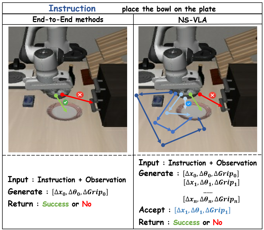
Figure 1: An example of the NS-VLA pipeline to execute instruction-conditioned manipulation by orchestrating symbolic primitives and sparse action chunks.

Figure 2: Success rate comparison under three training settings: (i) training on full demonstrations and testing on LIBERO, (ii) 1-shot training (one demonstration per task) and testing on LIBERO, and (iii) training on full demonstrations and testing on LIBERO-Plus. While most baselines achieve high SR with full-demo training, their performance drops sharply under low-data training and generalization tasks. In contrast, NS-VLA maintains a consistently high success rate with minimal performance degradation.

However, current VLA methods largely inherit the modeling and optimization of multimodal LLMs, which poses three major challenges: (i) Lack of structural awareness in end-to-end methods. Robotic manipulation is organized into reusable primitives shared across short and long-horizon tasks. However, end-to-end VLA methods rely on VLMs to directly generate action sequences without capturing internal connections, resulting in poor generalization capabilities. (ii) Heavy reliance on large-scale data and complex architectures. While pre-trained VLMs help generate actions, their success largely depends on complex models and massive demonstrations, but generating demonstrations for every task is impractical. (iii) Limited interaction with explorable environments. Although existing methods based on Supervised Fine-Tuning achieve high trajectory precision, they are limited to imitating expert trajectories, which restricts the model’s ability to explore the environment.

These considerations motivate us to propose a novel neuro-symbolic Vision-Language-Action (NS-VLA) framework, as shown in Figure 1, for structure-aware, efficient, and exploratory manipulation. First, we introduce a symbolic encoder to extract a structured primitive plan from inputs, which allows the model to capture relationships and shared structures across different tasks. Moreover, we propose a grounded symbolic solver for data-efficient action sequencing, thereby reducing reliance on complex architectures by generating actions through logical reasoning rather than direct regression. Furthermore, we implement an online RL objective that enables autonomous online environment exploration, jointly optimizing primitive classification and action generation via trajectory-task coupled reward design.

We perform extensive experiments on robotic benchmarks to assess learning capability and robustness to perturbations. As shown in Figure 2, the results demonstrate that NS-VLA outperforms previous methods across these challenging settings, while exhibiting higher data efficiency and an expanded exploration space. Our approach adopts a neuro-symbolic workflow (Wu et al., 2023) that captures the correlations between primitives, maintaining high efficiency with a lightweight structure. This work lays a foundation for building the next generation of neuro-symbolic embodied agents.

2 Related work

Neuro-Symbolic Methods for LLMs. Neuro-symbolic learning combines neural pattern recognition with symbolic reasoning to improve compositionality, interpretability, and verifiability (Mao et al., 2019; Gupta et al., 2019; Tian et al., 2022). In the context of LLMs, neuro-symbolic methods have developed along two directions. One line augments LLMs with external tools such as retrievers, calculators, code execution, planners, and specialized models to mitigate limitations in up-to-date knowledge, precise computation, and systematic reasoning (Pan et al., 2023; Luo et al., 2025b). Another line maps natural language to symbolic problem specifications and delegates inference to external solvers (Xu et al., 2025), often within self-improving loops that generate, verify, and refine reasoning trajectories. In this paper, we present a neuro-symbolic VLA framework that brings these principles into robotic manipulation.

VLA Models and RL for VLA Models. Recent VLA models commonly adopt large pretrained vision–language backbones and represent robot actions as discrete tokens, enabling end-to-end policy learning from visual observations and natural-language instructions (Ahn et al., 2022; Team et al., 2024; Liu et al., 2024; Li et al., 2025c; Song et al., 2025; O’Neill et al., 2024). OpenVLA (Kim et al., 2024) demonstrates the effectiveness of this paradigm by directly mapping multimodal inputs to low-level control actions. Recent works apply RL-based post-training to VLA models, leveraging verifiable or learned rewards to improve long-horizon decision-making and action consistency, thereby expanding the exploration space (Lu et al., 2025; Ye et al., 2025a; Li et al., 2025a, b; Gao et al., 2025).

Instruction clause	Primitive ops
place white mug on left plate	pickplace_on
place yellow-white mug on right plate	pickplace_on
place chocolate pudding right of plate	pickplace_rel
put yellow-white mug in microwave	pickplace_in
close microwave	close
turn on stove	turn_on
put alphabet soup in basket	pickplace_in
put book in caddy back compartment	pickplace_in

(a) Clause-to-primitive conversion examples.

(b) Primitive distribution.

Figure 3: (a) Examples of converting LIBERO instruction clauses into primitives and (b) the primitive distribution.

3 Preliminaries

Definition 1: Neuro. Neuro denotes differentiable components that map continuous observations to representations and actions. In NS-VLA, a pretrained VLM encodes $(x,o_{t}=\{I_{t},S_{t}\})$ into token features, which are consumed by learned modules for primitive inference and control(d’Avila Garcez and Lamb, 2020).

Definition 2: Symbolic. Symbolic denotes discrete primitives and structured constraints. We use a primitive set $\mathcal{U}$ and an episode-level plan $p=(u^{(1)},\ldots,u^{(M)})$, and track execution with a plan pointer $m_{t}$ under a monotone constraint to stabilize switching.

Problem Statement. In the VLA setting, given an instruction $x$ and observations ${o_{t}}$, the goal is to generate a sequence of continuous actions that accomplishes the task.

Figure 4: Overview of the NS-VLA framework: an RL-optimized neuro-symbolic policy for Robotic manipulation, where the agent hierarchically orchestrates visual grounding, symbolic primitive inference, and continuous action chunking.

4 Method: NS-VLA

In this section, we present NS-VLA, which consists of three tightly coupled components: (i) a neuro-symbolic encoding module that grounds language and perception into discrete primitives and compact state representations, (ii) a lightweight symbolic solver that translates the inferred primitives into efficient, real-time action generation, and (iii) an online reinforcement learning policy that refines the trainable modules in situ to improve task success under partial observability and sparse rewards.

4.1 Neuro-Symbolic Encoding and Embedding

As shown in Figure 4, NS-VLA follows the neuro-symbolic paradigm of PAL (Gao et al., 2023) and adapts it to VLA.

4.1.1 Neuro-Symbolic Encoder

Let $\mathcal{D}={(\tau_{i},x_{i},o_{i})}$ be a dataset of demonstrations, where $\tau_{i}$ denotes the $i$-th trajectory. Given an instruction $x$ and the current observation $o_{t}$, a pretrained VLM encoder is then applied to extract token-level features, which serve as the shared representation for planning and primitive inference:

$$\psi_{t}=\mathrm{Enc}_{\mathrm{VLM}}(o_{t},x)\in\mathbb{R}^{N\times d_{\psi}}.$$ (1)

Plan generation. At the beginning of an episode, the VLM produces a sequence of structured primitives as plan conditioned on the instruction and initial observation.

$$p=(u^{(1)},\ldots,u^{(M)}),\qquad u^{(m)}\in\mathcal{U},$$ (2)

Specifically, each primitive is a neuro-symbol that specifies what to manipulate and how to manipulate(Bacon et al., 2017; Vezhnevets et al., 2017). The plan is kept fixed throughout the episode to preserve temporal consistency.We model execution progress via a plan pointer $m_{t}\in\{1,\ldots,M\}$ and impose a monotone constraint:

$$m_{t}\in\{m_{t-1},\,\min(m_{t-1}+1,M)\}.$$ (3)

4.1.2 Symbolic Classifier

Given the encoded tokens $\psi_{t}$, we predict which primitive in the VLM plan is currently being executed. We first parameterize the symbolic classifier as an MLP $g_{\phi}$ that maps pooled VLM features to a distribution over plan primitives. Then, we pool tokens $\bar{\psi}_{t}=\mathrm{Pool}(\psi_{t})\in\mathbb{R}^{d_{\psi}}$ and compute:

$$p_{\phi}(u\mid\psi_{t})=\mathrm{softmax}\!\big(g_{\phi}(\bar{\psi}_{t})\big),\quad u\in\mathcal{U}.$$ (4)

Plan-constrained inference. Instead of selecting primitives freely, the decision is restricted to plan indices consistent with the monotone pointer prior. Let $\mathcal{K}(m_{t-1})$ denote the admissible index set; the resulting masked distribution over plan indices is

$$\mathcal{K}(m_{t-1}) =\{m_{t-1},\min(m_{t-1}+1,M)\},$$ (5)

$$\pi_{\phi}(k\mid\psi_{t},m_{t-1}) \propto p_{\phi}\!\left(u^{(k)}\mid\psi_{t}\right)\cdot\mathbf{1}\!\left[k\in\mathcal{K}(m_{t-1})\right].$$ (6)

The next plan pointer is obtained by maximizing the masked index distribution. The executed primitive is set to $\hat{u}_{t}=u^{(\hat{m}_{t})}$, and the pointer is updated as $m_{t}\leftarrow\hat{m}_{t}$. If the plan $p$ contains repeated primitives, ties are broken by preferring advancement, stabilizing segment boundaries.

$$\hat{m}_{t}=\operatorname*{argmax}_{k\in\mathcal{K}(m_{t-1})}\pi_{\phi}(k\mid\psi_{t},m_{t-1}).$$ (7)

Segment-end window supervision. The classifier is optimized with a transition-focused objective. For each demonstration segment of primitive $u_{k}$ ending at time $\tau_{k}^{\mathrm{end}}$, a short window $\mathcal{W}_{k}=\{\tau_{k}^{\mathrm{end}}-w,\ldots,\tau_{k}^{\mathrm{end}}\}$ is defined, and the weighted cross-entropy loss is minimized:

$$\mathcal{L}_{\mathrm{cls}}(\phi)=-\sum_{k}\sum_{t\in\mathcal{W}_{k}}\alpha_{u_{k}}\log p_{\phi}(u_{k}\mid\psi_{t}),$$ (8)

where $\alpha_{u_{k}}$ compensates for class imbalance. This supervision emphasizes boundary frames, sharpening transitions while down-weighting ambiguous intermediate states.

Proposition 4.1.

The plan-constrained update makes $m_{t}$ monotone with step size $\leq 1$, stabilizing segmentation and reducing flicker; deterministic tie-breaking yields a unique segmentation under repeats.

Proof.

We provide quantitative experimental results in Section 5.4 and qualitative proofs in Appendix B.1. ∎

4.2 Symbolic Solver

The symbolic solver translates the structured neuro-symbol $\hat{u}_{t}$ into continuous actions. To ensure real-time performance, we design a architecture that sparsifies visual inputs and generates actions in temporal chunks.

4.2.1 Visual Token Sparsification

Standard VLM encoders output a dense sequence of tokens $\psi_{t}=\{\psi_{t,i}\}_{i=1}^{N}$, which introduces computational redundancy(Ryoo et al., 2021; Rao et al., 2021; Bolya et al., 2022). We propose a query-driven(Jaegle et al., 2021) attention layer to retain only the visual patches relevant to the current neuro-symbol.

Query-conditioned filtration. The predicted primitive is embedded by separately encoding its object and operation components and then composing them into a query vector: $\mathbf{q}_{t}=\mathrm{Embed}(\hat{u}_{t})$. We then compute relevance scores:

$$\alpha_{t,i}=\frac{\mathbf{q}_{t}^{\top}W_{k}\mathbf{z}_{t,i}}{\sqrt{d_{z}}},i=1,\ldots,N.$$ (9)

Soft Top-$K$ during training. During training, we use a differentiable relaxation of Top-$K$ gating(Xie et al., 2020; Plötz and Roth, 2018). Let $\tau_{t,K}$ denote the $K$-th largest value of $\{\alpha_{t,i}\}_{i=1}^{N}$ (stop-gradient for stability), and define a soft gate

$$g_{t,i}=\sigma\!\left(\frac{\alpha_{t,i}-\tau_{t,K}}{\tau}\right)\in(0,1),i=1,\ldots,N,$$ (10)

where $\tau$ is a temperature. At inference time, we use the hard Top-$K$ set $\mathcal{I}_{t}=\mathrm{TopK}(\{\alpha_{t,i}\}_{i=1}^{N},K)$.

Sparse feature fusion. We normalize weights and aggregate selected tokens into a compact context vector:

$$w_{t,i}=\frac{\exp(\alpha_{t,i})\,g_{t,i}}{\sum_{j=1}^{N}\exp(\alpha_{t,j})\,g_{t,j}}.$$ (11)

$$\mathbf{c}_{t}=\sum_{i=1}^{N}w_{t,i}\,W_{v}\mathbf{z}_{t,i}.$$ (12)

where in inference $g_{t,i}=\mathbf{1}[i\in\mathcal{I}_{t}]$. This reduces the visual representation from $N$ tokens to a single vector $\mathbf{c}_{t}$.

4.2.2 Action Generator

A recurrent solver is replaced with a causal Transformer that maps sparse visual context and neuro-symbolic state to continuous robot actions. At each step, the solver token is formed by concatenating the sparse visual summary, the primitive embedding, and the proprioceptive state, $e_{t}=[\mathbf{c}_{t};\ \mathrm{Embed}(\hat{u}_{t});\ S_{t}]$. The model then outputs an open-loop action chunk(Zhao et al., 2023) of length $H$:

$$\mathbf{A}_{t}=(a_{t},\dots,a_{t+H-1})=\mathrm{Head}\!\left(\mathrm{Transformer}_{\theta}(e_{0:t})_{t}\right).$$ (13)

Proposition 4.2.

The solver improves online efficiency by query-conditioned Top-$K$ token sparsification and $H$-step chunked action generation, reducing visual redundancy and stabilizing real-time control.

Proof.

We provide quantitative experimental results in Section 5.5 and qualitative proofs in Appendix B.1. ∎

4.3 Online Reinforcement Learning Optimization

We formulate the online phase as a partially observable Markov decision process (POMDP) and optimize a history-dependent hierarchical policy over neuro-symbols and chunked actions(Kaelbling et al., 1998). Let

$$\Theta\triangleq\{\phi,\theta\}$$ (14)

denote the learnable parameters. To mitigate drift, the pretrained VLM encoder and plan generator are frozen, while lightweight modules are updated with KL regularization to a behavior-cloning reference policy(Schulman et al., 2017; Ng et al., 1999; Wiewiora, 2003).

4.3.1 RL Formulation

We model the problem as a POMDP $(\mathcal{S},\mathcal{A},\mathcal{O},\mathcal{T},\Omega,R,\gamma)$. At time $t$, the agent receives an observation $o_{t}\in\mathcal{O}$ and maintains a history $\mathcal{H}_{t}=(x,o_{0:t},a_{0:t-1})$. We use the VLM encoder to compute $\psi_{t}$ (Eq. 1) and the causal Transformer to summarize history. The hierarchical policy is

$$\pi_{\Theta}(u_{t},\mathbf{A}_{t}\mid\mathcal{H}_{t})=p_{\phi}(u_{t}\mid\psi_{t},m_{t-1})\cdot\pi_{\theta}(\mathbf{A}_{t}\mid e_{0:t}).$$ (15)

4.3.2 Primitive-Segmented Reward

Segmentation. Let $(\hat{m}_{t},\hat{u}_{t})$ be the plan-constrained prediction in Eq. 7. The segment index is defined as $\sigma_{t}=\hat{m}_{t}$, and a boundary is detected when the index changes, i.e., $b_{t}=\mathbf{1}[\sigma_{t}\neq\sigma_{t-1}]$.

Segment milestone reward. A segment-completion reward is assigned as $r_{t}^{\mathrm{seg}}=b_{t}$.

Within-segment progress shaping. For reward shaping, a compact latent is extracted using a frozen encoder(Fei et al., 2025a), $\ell_{t}=E_{\mathrm{w}}(o_{t})$.

For each segment index $\sigma$, we maintain $C$ reference prototypes $\{\mu_{\sigma,c}\}_{c=1}^{C}$ constructed from successful segments (Appendix C). We define a segment-conditioned potential

$$\Phi_{t}\triangleq-\min_{c}\|\ell_{t}-\mu_{\sigma_{t},c}\|_{2},$$ (16)

and a progress reward by potential difference:

$$r_{t}^{\mathrm{prog}}=\gamma\Phi_{t+1}-\Phi_{t},r_{t}=r_{t}^{\mathrm{task}}+\lambda_{\mathrm{seg}}r_{t}^{\mathrm{seg}}+\lambda_{\mathrm{prog}}r_{t}^{\mathrm{prog}}.$$ (17)

Here $r_{t}^{\mathrm{task}}$ is the sparse task signal. Prototypes are treated as constants within each policy update.

4.3.3 Group-Relative Optimization Strategy

We optimize parameters using GRPO(Shao et al., 2024) with group-normalized advantages. For each instruction, we collect a group of $G$ rollouts and compute

$$A_{i}=\frac{R_{i}-\mathrm{Mean}(\{R_{j}\})}{\mathrm{Std}(\{R_{j}\})+\epsilon}.$$ (18)

To prevent policy collapse during online optimization, we penalize deviation from a behavior-cloning reference policy $\pi_{\mathrm{BC}}$, which serves as a stable behavioral prior:

$$\mathcal{J}_{\text{GRPO}}(\Theta)=\frac{1}{G}\sum_{i=1}^{G}\Big[r_{i}(\Theta)A_{i}-\beta\mathrm{D_{KL}}\big(\pi_{\Theta}\|\pi_{\text{BC}}\big)\Big],$$ (19)

where $r_{i}(\Theta)$ is the standard trajectory-level importance ratio. The KL term constrains policy updates to remain close to the reference policy, improving stability under sparse rewards(Schulman et al., 2015; Wu et al., 2019; Fujimoto and Gu, 2021; Ouyang et al., 2022). Full pseudocode and training details are provided in Appendix C.

Proposition 4.3.

With fixed prototypes per update, the within-segment progress term is potential-based shaping on a segment-augmented process and preserves optimal policies; KL anchoring limits drift from the behavior-cloning reference, stabilizing online updates under sparse rewards.

Proof.

We provide quantitative experimental results in Section 5.6 and qualitative proofs in Appendix B.1. ∎

Table 1: Main results on LIBERO benchmarks. Blocks reports Success Rate (SR%) and the average number of steps to success (Steps) on different task subsets.

Evaluation on the LIBERO benchmark
Method	Params	Spatial	Object	Goal	Long	Avg.
# Trained on LIBERO under the one-trajectory-per-task (1-shot) training regime
ACT (Zhao et al., 2023)	–	8.0(–)	15.8(–)	5.4(–)	0.0(–)	7.3(–)
DP (Han et al., 2024)	–	19.8(–)	28.4(–)	20(–)	0.8(–)	17.2(–)
BAKU (Haldar et al., 2024)	–	42.2(–)	65.0(–)	30.3(–)	4.6(–)	35.5(–)
OpenVLA (Kim et al., 2024)	7B	47.4(↓37.3)	46.0(↓42.4)	44.3(↓34.9)	4.9(↓48.8)	35.7(↓40.8)
$\pi 0$ (Black et al., 2024b)	3B	48.6(↓48.2)	47.2(↓51.6)	33.2(↓62.6)	20.4(↓64.8)	37.4(↓56.8)
SEIL (Ye et al., 2025b)	–	53.2(–)	82.0(–)	49.2(–)	14.6(–)	49.7(–)
OpenVLA-OFT (Kim et al., 2025)	7B	63.6(↓34.0)	54.9(↓43.5)	59.6(↓38.3)	17.3(↓77.2)	48.9(↓48.2)
UniVLA (Bu et al., 2025)	7B	70.7(↓25.8)	59.6(↓37.2)	65.4(↓30.2)	24.5(↓67.5)	55.1(↓40.1)
EVOLVE-VLA (Bai et al., 2025)	7B	73.4(↓22.0)	70.0(↓27.4)	64.7(↓31.1)	37.1(↓57.3)	61.3(↓34.5)
VLA-Adapter (Wang et al., 2025)	0.5B	80.6(↓19.0)	71.6(↓28.0)	69.8(↓28.7)	39.2(↓57.2)	65.3(↓33.2)
NS-VLA (ours)	2B	85.7(↓13.8)	75.3(↓24.3)	70.7(↓27.8)	45.2(↓51.6)	69.1(↓29.5)
Evaluation on the LIBERO-Plus benchmark
# Trained on the full LIBERO dataset
OpenVLA (Kim et al., 2024)	7B	19.4(↓65.3)	14.0(↓74.4)	15.1(↓64.1)	14.3(↓39.4)	15.6(↓60.9)
WorldVLA (Cen et al., 2025)	7B	32.5(↓55.1)	28.6(67.6)	31.8(↓51.6)	8.2(↓51.8)	25.0(↓56.8)
NORA (Hung et al., 2025)	3B	47.6(↓44.6)	34.4(↓61)	38.8(↓50.6)	36.3(↓38.3)	39.0(↓48.9)
UniVLA (Bu et al., 2025)	7B	55.5(↓41.0)	36.7(↓60.1)	40.7(↓54.9)	39.9(↓52.1)	42.9(↓52.3)
VLA-Adapter (Wang et al., 2025)	0.5B	84.7(↓14.9)	46.3(↓53.3)	54.5(↓43.7)	51.4(↓45.0)	58.9(↓39.6)
$\pi 0$ (Black et al., 2024b)	3B	60.7(↓36.1)	61.4(↓37.4)	44.9(↓50.9)	48.4(↓36.8)	53.6(↓40.6)
$\pi 0$-Fast (Pertsch et al., 2025)	3B	74.4(↓22.0)	72.7(↓24.1)	57.5(↓31.1)	43.4(↓16.8)	61.6(↓23.9)
RIPT-VLA (Tan et al., 2025)	7B	85.8(↓9.8)	64.3(↓34.1)	58.0(↓34.7)	67.5(↓18.2)	68.4(↓25.2)
OpenVLA-OFT (Kim et al., 2025)	7B	84.0(↓13.6)	66.5(↓31.9)	63.0(↓34.9)	66.4(↓28.1)	69.6(↓27.5)
NS-VLA (ours)	2B	88.1(↓11.4)	79.0(↓20.6)	70.2(↓28.5)	80.3(↓17.0)	79.4(↓19.2)

5 Experiments

This section presents the experimental setup, results, and analysis. We answer the following research questions (RQs): RQ1: Does NS-VLA outperform other VLA methods? RQ2: Does the main component of NS-VLA work, and how is its comparative analysis? RQ3-5: How are data efficiency, generalizability, and exploration space of NS-VLA?

Method	LIBERO AVG. SR(%)$\uparrow$
NS-VLA	98.6
w/o P.C.	79.7
w/o V.E.	90.1
w/o A.G.	85.2
w/o R.L.	91.6
-no Traj.Reward	94.6
-no Task.Reward	92.8

(a)

(b)

(c)

(d)

Figure 5: (a) Ablation study of NS-VLA. (b) Robustness analysis under environmental perturbations. (c) Attention heatmap visualization validating the Vision Extractor. (d) Comparative training curves against the GRPO.

5.1 Experimental Setup

Datasets. All experiments are conducted on three robot datasets in a low-resource setting: LIBERO (Liu et al., 2023), LIBERO-Plus (Fei et al., 2025b), and CALVIN (Mees et al., 2022). We additionally annotate datasets with primitives. Details of the annotation are provided in Appendix D.

Baselines. We mainly compare our method with OpenVLA (Kim et al., 2024), $\pi 0$ (Black et al., 2024b), OpenVLA-OFT (Kim et al., 2025), UniVLA (Bu et al., 2025), and VLA-Adapter (Wang et al., 2025) with the same low-resource setting. More baseline details are provided in Appendix E.

Evaluation Metrics. In line with prior studies, we use Success Rate (SR) as the evaluation metric for LIBERO and LIBERO-Plus. For CALVIN, we report the 5-task success rate and average sequence length, which measure the probability of consecutively completing five tasks and the average number of tasks successfully completed in a row.

Implementation Details. Following LIBERO-Plus, we conduct 1-shot experiments on LIBERO, utilizing only one demonstration per task as the training set to evaluate the success rates of all baselines. Furthermore, we employ the full LIBERO demonstrations for training and evaluate success rates across all tasks in LIBERO-Plus.

5.2 Main Results (RQ1)

As shown in Table 1, we compare NS-VLA with baselines in different settings. In addition, we have two key observations regarding data utilization and model generalization.

Data Efficiency in One-Shot Settings. When trained with only a single demonstration trajectory selected per task from LIBERO, NS-VLA not only consistently achieves the highest success rates across all tasks but also exhibits the minimal performance degradation compared to its counterpart trained on the full demonstration(Finn et al., 2017; Zhao et al., 2024). This minimal drop in success rate highlights the data efficiency of NS-VLA, demonstrating its capability to capture correlations in different tasks from scarce data to maintain robust performance, whereas baseline methods suffer significant deterioration.

Robustness Against Environmental Perturbations. We further assess the resilience of the models by evaluating policies trained on the full LIBERO dataset on the challenging LIBERO-Plus benchmark, which introduces rigorous perturbations including variations in lighting, texture, and spatial layout. In this highly dynamic setting, NS-VLA not only sustains the highest success rates among all baselines but also incurs the minimum average performance decay relative to the standard testing environment(Bodnar et al., 2019). This superior stability suggests that NS-VLA successfully captures the invariant associations between task primitives and scene contexts, enabling precise task completion even in the presence of significant visual and spatial disturbances.

Model	LIBERO
	Success Rate (%)	Primitive Accuracy (%)
Qwen3-VL-8B	98.9	95.5
Qwen3-VL-4B	98.8	94.3
Qwen3-VL-2B	98.6	94.1

(a)

(b)

Figure 6: Efficiency Analysis. (a) Impact of pretrained VLM parameter sizes on Success Rate(%) and Primitive Accuracy(%). (b) Impact of varying training data on the model’s learning curves.

5.3 Ablation Study and Comparative Analysis (RQ2)

As shown in Figures 5, we conduct an ablation study and comparative analysis on NS-VLA.

Ablation Study. We remove four components of NS-VLA: primitive classifier (P.C.), vision extractor (V.E.), action generator (A.G.) and reinforcement learning (R.L.), to assess their individual contributions. As shown in Figure 5(a), removing any module leads to performance degradation.

Structural Robustness via Primitive Decomposition. As shown in Figure 5(b), ablating either the Primitive Classifier or the Action Generator results in a marked performance decline under the diverse environmental perturbations of LIBERO-Plus(Fei et al., 2025b). This empirical evidence underscores two critical insights: (i) the Primitive Classifier is pivotal for high-quality generation, as it grounds continuous control by identifying the active atomic operation state; and (ii) the Action Generator, functioning as a symbolic solver, exhibits robustness against distribution shifts compared to unstructured end-to-end decoding, effectively mitigating error accumulation in dynamic environments.

Method	Calvin ABC$\rightarrow$D
	5-Task SR$\uparrow$	Avg. Length$\uparrow$
OpenVLA	43.5	3.27
UniVLA	56.5	3.80
OpenVLA-OFT	66.5	4.10
VLA-Adapter	80.0	4.50
NS-VLA (Ours)	91.2	4.72

(a)

(b)

Figure 7: Generalizability Analysis. (a) Zero-shot generalization performance on CALVIN ABC$\to$D split. (b) Performance comparison against baselines on LIBERO-Plus under perturbations.

(a)

(b)

Figure 8: Exploration Analysis. (a) Comparative case study of trajectory generation: End-to-End VLA methods vs. NS-VLA. (b) Visualization of exploration space coverage across different VLA paradigms.

Efficacy of Task-Relevant Visual Grounding. Referring to Figures 5(a) and (c), the Vision Extractor plays a crucial role in attention mechanisms. By dynamically attending to visual regions strictly relevant to the current primitive’s arguments, this module effectively filters out background distractions and visual noise. This component also significantly enhances the model’s resilience to visual perturbations, ensuring that control signals remain conditioned on salient task features rather than spurious correlations.

Optimization Stability with $\mathcal{J}_{\text{GRPO}}$. Figure 5(d) compares different reinforcement learning strategies. The proposed soft-constrained objective $\mathcal{J}_{\text{GRPO}}$ outperforms the GRPO baseline, achieving higher success rates with fewer training iterations. This confirms that incorporating the trust-region constraint within the group-relative optimization framework facilitates more stable convergence and produces stronger VLA action generation capabilities, establishing $\mathcal{J}_{\text{GRPO}}$ as a favorable choice for training VLA agents.

5.4 Analysis of NS-VLA’s Data Efficiency (RQ3)

As shown in Figure 6(a) and (b), NS-VLA maintains high success rates across varying backbone sizes, indicating effective neuro-symbolic disentanglement. Moreover, comparing one-shot against full-demonstration training, NS-VLA exhibits accelerated convergence with minimal performance degradation. This confirms the symbolic plan prior serves as a strong inductive bias, significantly reducing data and annotation costs while preserving core capabilities.

5.5 Analysis of NS-VLA’s Generalizability (RQ4)

As shown in Figure 7(a) and (b), we assess zero-shot generalizability of NS-VLA on the CALVIN ABC$\to$D and the 7-dimensional perturbation suite of LIBERO-Plus. On CALVIN, NS-VLA surpasses the state-of-the-art by boosting the 5-chain success rate by 11.2% and achieving a significantly longer average sequence length. Furthermore, under the environmental perturbations of LIBERO-Plus, our model sustains an average success rate markedly superior to baselines across all metrics. These results confirm that NS-VLA effectively internalizes intrinsic task associations and robustly maps this structural knowledge to zero-shot scenarios, demonstrating exceptional generalizability.

5.6 Analysis of NS-VLA’s Exploration Space (RQ5)

As shown in Figure 8(a), we compare the exploration boundaries of NS-VLA’s online RL against Diffusion, Flow Matching, and End-to-End VLA methods. The results quantitatively indicate that the Online RL enables significantly broader action coverage than the comparative methods, achieving active and extensive environmental exploration.

Case Study Analysis. As shown in Figure 8(b), we present a comparative trajectory generation study between end-to-end methods and NS-VLA. While end-to-end approaches typically infer and execute a single deterministic trajectory without intermediate verification, NS-VLA explores a distribution of potential candidate trajectories to identify and execute the optimal path. This mechanism not only ensures superior exploration quality but also facilitates robust generalization in data-scarce regimes by explicitly filtering out suboptimal behaviors before interaction.

6 Conclusion

In this paper, we introduced NS-VLA, a novel neuro-symbolic Vision-Language-Action framework trained via online reinforcement learning. By integrating a symbolic encoding scheme with a data-efficient solver and online RL-based exploration, our approach effectively addresses the limitations of existing VLA models in learning reusable primitives and handling data scarcity. Extensive experiments on robotic manipulation benchmarks demonstrate that NS-VLA outperforms previous methods in both one-shot training and data-perturbed settings, while simultaneously exhibiting superior zero-shot generalizability, high data efficiency, and an expanded exploration space. These results highlight the promise of combining neuro-symbolic reasoning with reinforcement learning to build more robust, efficient, and generalizable embodied agents. We believe this framework, which shifts VLA toward structured reasoning, establishes a new standard for data-efficient robotic learning.

7 Impact Statement

This work introduces NS-VLA, a novel neuro-symbolic framework for robotic manipulation via online reinforcement learning. While effective, it still faces limitations in the manual definition of action primitives and the scalability of sim-to-real transfer. To address these challenges, we outline four future directions: (1) refining primitive granularity via automatic discovery, (2) evolving the architecture for tighter neuro-symbolic integration, (3) scaling validation to diverse real-world environments, and (4) enabling lifelong learning with human-interactive correction, as detailed in Section H. This work poses no immediate ethical concerns, as it currently relies on standard simulation benchmarks. However, as the field moves toward physical deployment, strict safety protocols must be established to ensure safe human-robot interaction. We aim to advance general-purpose robotic technology with positive societal impacts.

Appendix

Appendix A Prompt used in NS-VLA

Figure 9 shows the system prompt used to elicit structured primitive plans from the VLM. Given the language instruction and the current observation, the model is instructed to output only a JSON array of steps, where each step specifies an operation (op) and its arguments (args). This strict output contract enables reliable parsing into the symbolic plan representation $p=(u^{(1)},\ldots,u^{(M)})$. By explicitly forbidding extra fields and free-form text, the prompt reduces formatting variance and improves the stability of downstream decoding.

Figure 9: Prompt template used for structured plan generation in NS-VLA.

Appendix B Proof

B.1 Proof of Proposition 4.1

We prove that the plan-constrained pointer update produces a monotone execution trace that advances by at most one index per decision step. This implies a stable left-to-right plan traversal and eliminates backward switching, which is the main source of temporal flickering.

Setup and notation.

Let the instruction-conditioned plan be $\mathbf{p}(x)=\{u^{(1)},\ldots,u^{(M)}\}$. The plan pointer at decision step $t$ is $m_{t}\in\{1,\ldots,M\}$. Given $m_{t-1}$, define the admissible index set

$$\mathcal{K}(m_{t-1})=\big\{m_{t-1},\,\min(m_{t-1}+1,M)\big\}.$$ (20)

The masked index policy (Eq. 6) is

$$\pi_{\phi}(k\mid\psi_{t},m_{t-1})=\frac{p_{\phi}(u^{(k)}\mid\psi_{t})\,\mathbf{1}[k\in\mathcal{K}(m_{t-1})]}{\sum_{j\in\mathcal{K}(m_{t-1})}p_{\phi}(u^{(j)}\mid\psi_{t})}.$$ (21)

The constrained decoding rule (Eq. 7) selects

$$\hat{m}_{t}\in\arg\max_{k\in\mathcal{K}(m_{t-1})}\pi_{\phi}(k\mid\psi_{t},m_{t-1}),\qquad m_{t}\leftarrow\hat{m}_{t}.$$ (22)

Lemma 1: Support of the masked policy.

For any $t$ and any $m_{t-1}$, $\pi_{\phi}(\cdot\mid\psi_{t},m_{t-1})$ assigns zero probability to indices outside $\mathcal{K}(m_{t-1})$.

$$\forall k\notin\mathcal{K}(m_{t-1}),\quad\pi_{\phi}(k\mid\psi_{t},m_{t-1})=0.$$ (23)

Proof. By Eq. 21, the numerator contains $\mathbf{1}[k\in\mathcal{K}(m_{t-1})]$, hence it is zero for $k\notin\mathcal{K}(m_{t-1})$. The denominator is strictly positive since it sums nonnegative terms and $\mathcal{K}(m_{t-1})$ is nonempty. ∎

Lemma 2: One-step admissibility of decoding.

The decoded index must lie in the admissible set:

$$\hat{m}_{t}\in\mathcal{K}(m_{t-1})=\{m_{t-1},\min(m_{t-1}+1,M)\}.$$ (24)

Proof. Eq. 22 maximizes $\pi_{\phi}(\cdot\mid\psi_{t},m_{t-1})$ over $k\in\mathcal{K}(m_{t-1})$, so $\hat{m}_{t}\in\mathcal{K}(m_{t-1})$ holds by construction. ∎

Lemma 3: Invariance of the pointer range.

Assume $m_{t-1}\in\{1,\ldots,M\}$. Then $m_{t}\in\{1,\ldots,M\}$.

Proof. By Lemma 2, $m_{t}\in\mathcal{K}(m_{t-1})$. From Eq. 20, both elements of $\mathcal{K}(m_{t-1})$ lie in $\{1,\ldots,M\}$. ∎

Main claim: monotonicity and at-most-one advance.

From Lemma 2 and the explicit form of $\mathcal{K}(m_{t-1})$,

$$m_{t}\in\{m_{t-1},\,\min(m_{t-1}+1,M)\}\quad\Longrightarrow\quad m_{t}\geq m_{t-1}\ \ \text{and}\ \ m_{t}-m_{t-1}\in\{0,1\}.$$ (25)

Thus $\{m_{t}\}$ is non-decreasing and advances by at most one per decision step. In particular, backward switching $m_{t}<m_{t-1}$ is impossible, which removes oscillations between earlier and later primitives.

Induction over time.

Let $m_{0}\in\{1,\ldots,M\}$. By Lemma 3, $m_{1}\in\{1,\ldots,M\}$. Repeating the same argument yields $m_{t}\in\{1,\ldots,M\}$ for all $t$, while Eq. 25 holds at every step, proving the proposition.

Remark on repeated primitives and deterministic trace.

If $u^{(i)}=u^{(j)}$ for $i\neq j$, multiple maximizers may exist. With a deterministic tie-breaking rule, such as preferring the larger index when scores are equal, $\hat{m}_{t}$ becomes unique. Therefore the boundary indicator $b_{t}=\mathbf{1}[m_{t}\neq m_{t-1}]$ and the induced segmentation are reproducible, which is useful for segment-level accounting and consistent reward assignment.

∎

B.2 Proof of Proposition 4.2

We formalize efficiency gains from two orthogonal reductions: token count reduction through query-conditioned sparsification, and decision count reduction through chunked action generation.

Setup.

Let $N$ be the number of VLM tokens per step, and $K\ll N$ be the selected token budget. Let $H$ be the chunk horizon and $T$ be the number of low-level environment steps in an episode. We analyze computation at the granularity of one decision step, then lift it to an episode.

Part I: Token sparsification reduces solver-side complexity.

Relevance scoring (Eq. 9) computes scores $\{\alpha_{t,i}\}_{i=1}^{N}$. Assume token dimension is $d$ and the scoring uses a constant number of query vectors. Then the scoring pass costs

$$C_{\mathrm{score}}(N)=O(Nd).$$ (26)

After Top-$K$ selection, the solver consumes only $\tilde{\mathbf{Z}}_{t}$ with $|\tilde{\mathbf{Z}}_{t}|=K$. Consider a generic solver block that performs cross-attention between a constant number of queries and the token set. Its cost scales linearly in the token count:

$$C_{\mathrm{attn}}(n)=O(nd).$$ (27)

Hence, replacing $N$ by $K$ yields a reduction factor of approximately $N/K$ for solver-side attention. If the solver has $L$ such blocks, the per-decision compute is

$$C_{\mathrm{dense}}=L\,C_{\mathrm{attn}}(N)=O(LNd),\qquad C_{\mathrm{sparse}}=C_{\mathrm{score}}(N)+L\,C_{\mathrm{attn}}(K)=O(Nd+LKd).$$ (28)

When $K\ll N$ and $L$ is not tiny, $C_{\mathrm{sparse}}$ is substantially smaller than $C_{\mathrm{dense}}$. The key point is that after sparsification, all deeper solver layers depend on $K$ rather than $N$.

Part II: Chunking reduces the number of decisions.

The solver emits an open-loop chunk of length $H$ per decision (Eq. 13). An episode with $T$ low-level steps requires only

$$T_{H}=\left\lceil\frac{T}{H}\right\rceil$$ (29)

high-level solver invocations, instead of $T$. Thus chunking reduces the number of expensive forward passes by a factor close to $H$.

Episode-level bound.

Combining Eq. 28 and Eq. 29, the episode compute satisfies

$$\text{Cost}_{\mathrm{sparse+chunk}}=T_{H}\cdot O(Nd+LKd),\qquad\text{Cost}_{\mathrm{dense+step}}=T\cdot O(LNd).$$ (30)

Therefore, sparsification reduces per-decision token dependence from $N$ to $K$, and chunking reduces decision count from $T$ to $T_{H}$. Together they improve inference throughput and reduce latency under long-horizon tasks.

∎

B.3 Proof of Proposition 4.3

This proof has two parts. First, we show that the dense within-segment progress reward can be written as potential-based shaping on an augmented process, which preserves optimal policies on that process. Second, we show that KL anchoring bounds the deviation between the updated policy and the reference policy, and therefore limits trajectory drift.

Potential-based shaping preserves optimal policies.

Augmented Markov process. Let the environment state be $s_{t}$. Let $\sigma_{t}$ denote the segment index used by the agent at time $t$, such as $\sigma_{t}=\hat{m}_{t}$. Define the augmented state

$$\tilde{s}_{t}=(s_{t},\sigma_{t}).$$ (31)

Given a fixed plan and fixed tie-breaking, the pointer update is deterministic given the agent history, so $\sigma_{t}$ can be treated as part of the augmented dynamics for the purpose of reward shaping. Within one policy update, we hold any prototype statistics used inside $\Phi$ fixed, so the potential is stationary during that update.

Potential function and shaping term. Let $\Phi:\tilde{\mathcal{S}}\rightarrow\mathbb{R}$ be bounded, and define a shaping reward

$$F(\tilde{s}_{t},\tilde{s}_{t+1})=\gamma\Phi(\tilde{s}_{t+1})-\Phi(\tilde{s}_{t}).$$ (32)

The shaped reward is $r^{\prime}_{t}=r_{t}+F(\tilde{s}_{t},\tilde{s}_{t+1})$. Your progress reward $r_{t}^{\mathrm{prog}}$ matches Eq. 32 by definition in the method section.

Value shift identity. For any history-dependent policy $\pi$, define values on the augmented process:

$$V^{\pi}(\tilde{s})=\mathbb{E}_{\pi}\!\left[\sum_{t\geq 0}\gamma^{t}r_{t}\mid\tilde{s}_{0}=\tilde{s}\right],\quad V^{\prime\pi}(\tilde{s})=\mathbb{E}_{\pi}\!\left[\sum_{t\geq 0}\gamma^{t}r^{\prime}_{t}\mid\tilde{s}_{0}=\tilde{s}\right].$$ (33)

Then

$$V^{\prime\pi}(\tilde{s}) =\mathbb{E}_{\pi}\!\left[\sum_{t\geq 0}\gamma^{t}\big(r_{t}+\gamma\Phi(\tilde{s}_{t+1})-\Phi(\tilde{s}_{t})\big)\right]$$

$$=V^{\pi}(\tilde{s})+\mathbb{E}_{\pi}\!\left[\sum_{t\geq 0}\gamma^{t+1}\Phi(\tilde{s}_{t+1})-\sum_{t\geq 0}\gamma^{t}\Phi(\tilde{s}_{t})\right]$$

$$=V^{\pi}(\tilde{s})-\Phi(\tilde{s})+\lim_{T\to\infty}\gamma^{T+1}\mathbb{E}_{\pi}\!\left[\Phi(\tilde{s}_{T+1})\right].$$ (34)

Since $\Phi$ is bounded and $\gamma\in(0,1)$, the limit term vanishes, hence

$$V^{\prime\pi}(\tilde{s})=V^{\pi}(\tilde{s})-\Phi(\tilde{s}).$$ (35)

Similarly for action values,

$$Q^{\prime\pi}(\tilde{s},a)=Q^{\pi}(\tilde{s},a)-\Phi(\tilde{s}).$$ (36)

The shift is independent of $a$, therefore the greedy action set is unchanged:

$$\arg\max_{a}Q^{\prime\pi}(\tilde{s},a)=\arg\max_{a}Q^{\pi}(\tilde{s},a),\qquad\forall\tilde{s}.$$ (37)

Thus potential-based shaping preserves optimal policies on the augmented process.

Remark on partial observability. If the environment is partially observable, one may treat the policy state as the full history $\mathcal{H}_{t}$. Then the same derivation applies by defining $\Phi$ on the information state $(\mathcal{H}_{t},\sigma_{t})$, as long as $\Phi$ is held fixed during a policy update.

KL anchoring bounds policy and trajectory drift.

Step-wise distribution bound. For any conditioning variable $c$ and two distributions $P,Q$, Pinsker’s inequality gives

$$\mathrm{TV}(P,Q)\leq\sqrt{\tfrac{1}{2}\mathrm{KL}(P\|Q)}.$$ (38)

Applying Eq. 38 to $P=\pi_{\Theta}(\cdot\mid c)$ and $Q=\pi_{\Theta_{\mathrm{ref}}}(\cdot\mid c)$ yields a direct conversion from the KL penalty to a total-variation bound.

From policy drift to return drift. Assume rewards are bounded: $|r_{t}|\leq R_{\max}$. Then for any policy, $|Q^{\pi}(\tilde{s},a)|\leq\frac{R_{\max}}{1-\gamma}$ and $|A^{\pi}(\tilde{s},a)|\leq\frac{2R_{\max}}{1-\gamma}$. Using the performance difference lemma on the augmented process,

$$J(\pi)-J(\pi_{\mathrm{ref}})=\frac{1}{1-\gamma}\,\mathbb{E}_{\tilde{s}\sim d_{\pi}}\,\mathbb{E}_{a\sim\pi(\cdot\mid\tilde{s})}\!\left[A^{\pi_{\mathrm{ref}}}(\tilde{s},a)\right],$$ (39)

where $d_{\pi}$ is the discounted state occupancy. Combining with Eq. 38 yields

$$|J(\pi)-J(\pi_{\mathrm{ref}})|\leq\frac{2R_{\max}}{(1-\gamma)^{2}}\,\mathbb{E}_{\tilde{s}\sim d_{\pi}}\sqrt{\tfrac{1}{2}\mathrm{KL}\!\left(\pi(\cdot\mid\tilde{s})\,\|\,\pi_{\mathrm{ref}}(\cdot\mid\tilde{s})\right)}.$$ (40)

Therefore, a KL penalty controls step-wise policy deviation and upper-bounds the induced drift in expected return and trajectory distribution. This is the formal sense in which KL anchoring stabilizes optimization in sparse-reward regimes.

∎

Appendix C Reinforcement Learning Algorithm Details

This appendix provides pseudocode for the online RL stage (Sec. 4.3) and practical strategies used to stabilize and scale optimization with chunked control and neuro-symbolic primitives. For clarity, we distinguish decision steps (indexed by $t$) from environment steps(Sutton et al., 1999): each decision outputs one $H$-step action chunk that is executed open-loop. Thus, the rollout buffer stores chunk-level tuples, while the environment transitions internally for $H$ low-level steps between two decision points.

Algorithm 1 NS-VLA for Online Optimization

0: Instruction-conditioned environment sampler $\mathcal{E}$; pretrained VLM encoder $\mathrm{Enc}_{\mathrm{VLM}}$ (frozen); episode-level plan generator producing $p=(u^{(1)},\dots,u^{(M)})$ (frozen); frozen shaping encoder $E_{\mathrm{w}}$; per-primitive prototype set $\{\mu_{\sigma,c}\}$ (refreshed periodically; treated as constant within an update); primitive classifier $p_{\phi}(u\mid\psi_{t})$ with plan-constrained inference (Eq. 7); solver policy $\pi_{\theta}(\mathbf{A}_{t}\mid\hat{u}_{t},\mathbf{c}_{t},S_{t})$; behavior-cloning reference policy $\pi_{\mathrm{BC}}$ (frozen); chunk horizon $H$; group size $G$; discount $\gamma$; KL weight $\beta$; step size $\alpha$; reward weights $\lambda_{\mathrm{seg}},\lambda_{\mathrm{prog}}$.

1: Initialize $\Theta\leftarrow\{\phi,\theta\}$ using lightweight supervised pretraining (Appendix C.2)

2: Set $\Theta_{\text{old}}\leftarrow\Theta$

3: Initialize per-primitive successful-segment buffers $\{\mathcal{B}_{\sigma}\}_{\sigma=1}^{M}$ and prototypes $\{\mu_{\sigma,c}\}$

4: for iteration $=1,2,\dots$ do

5:  (Optional) Refresh prototypes $\{\mu_{\sigma,c}\}$ from buffers $\{\mathcal{B}_{\sigma}\}$ (e.g., every $U$ iterations)

6:  Sample an instruction $x$ and initialize environment $\mathcal{E}(\cdot\,;x)$

7:  for $i=1$ to $G$ do

8:   Reset env; observe initial $o_{0}=\{I_{0},S_{0}\}$; set plan pointer $m_{0}\leftarrow 1$

9:   Generate episode plan $p\leftarrow(u^{(1)},\dots,u^{(M)})$ using the frozen plan generator (Sec. 4.1.1)

10:   Initialize trajectory buffer $\tau_{i}\leftarrow\emptyset$

11:   while not terminal do

12:    Observe $o_{t}=\{I_{t},S_{t}\}$ and compute tokens $\psi_{t}=\mathrm{Enc}_{\mathrm{VLM}}(o_{t},x)$ (Eq. 1)

13:    Infer $\hat{m}_{t}$ via Eq. 7 and set $\hat{u}_{t}=u^{(\hat{m}_{t})}$

14:    Compute boundary indicator $b_{t}\leftarrow\mathbf{1}[\hat{m}_{t}\neq m_{t-1}]$

15:    Sparsify visual tokens conditioned on $\hat{u}_{t}$ and obtain $\mathbf{c}_{t}$ (Eqs. 9–12)

16:    Compute shaping latent $\ell_{t}\leftarrow E_{\mathrm{w}}(o_{t})$

17:    Compute potential $\Phi_{t}\leftarrow-\min_{c}\|\ell_{t}-\mu_{\hat{m}_{t},c}\|_{2}$ (Eq. 16)

18:    Sample an action chunk $\mathbf{A}_{t}\sim\pi_{\theta_{\text{old}}}(\cdot\mid\hat{u}_{t},\mathbf{c}_{t},S_{t})$ (Eq. 13)

19:    (Optional) Record $\log\pi_{\theta_{\text{old}}}(\mathbf{A}_{t}\mid\hat{u}_{t},\mathbf{c}_{t},S_{t})$ for importance weighting

20:    Execute $\mathbf{A}_{t}$ open-loop for $H$ env steps; receive sparse task feedback $r_{t}^{\mathrm{task}}$

21:    Observe next boundary observation $o_{t+1}$ and compute $\ell_{t+1}\leftarrow E_{\mathrm{w}}(o_{t+1})$, $\Phi_{t+1}$

22:    Set segment reward $r_{t}^{\mathrm{seg}}\leftarrow b_{t}$

23:    Compute shaped reward $r_{t}\leftarrow r_{t}^{\mathrm{task}}+\lambda_{\mathrm{seg}}r_{t}^{\mathrm{seg}}+\lambda_{\mathrm{prog}}(\gamma\Phi_{t+1}-\Phi_{t})$ (Eq. 17)

24:    Append $(\psi_{t},\hat{m}_{t},\hat{u}_{t},\mathbf{c}_{t},S_{t},\mathbf{A}_{t},r_{t},b_{t},\ell_{t})$ to $\tau_{i}$

25:    Update pointer $m_{t}\leftarrow\hat{m}_{t}$

26:   end while

27:   Compute trajectory return $R_{i}\leftarrow\sum_{t}\gamma^{t}r_{t}$

28:   Update successful-segment buffers from $\tau_{i}$

29:   Parse $\tau_{i}$ into primitive segments using boundary indicators $b_{t}$

30:   for all segments with index $\sigma$ and end time $t_{e}$ do

31:    Compute segment summary $\bar{\ell}_{\sigma}\leftarrow\mathrm{Mean}(\{\ell_{t}\ \text{in segment}\})$

32:    if $b_{t_{e}}=1$ and $r_{t_{e}}^{\mathrm{task}}>0$ then

33:     Insert $\bar{\ell}_{\sigma}$ into buffer $\mathcal{B}_{\sigma}$ (with FIFO cap)

34:    end if

35:   end for

36:  end for

37:  Compute group advantages $\{A_{i}\}_{i=1}^{G}$ using Eq. 18

38:  Policy update (maximize Eq. 19)

39:  for $i=1$ to $G$ do

40:   Compute $\log\pi_{\Theta}(\tau_{i})$ and $\log\pi_{\Theta_{\text{old}}}(\tau_{i})$ under the joint policy (Eq. 15)

41:   Compute importance ratio $r_{i}(\Theta)=\exp\!\big(\log\pi_{\Theta}(\tau_{i})-\log\pi_{\Theta_{\text{old}}}(\tau_{i})\big)$

42:   Estimate KL penalty $\mathrm{D_{KL}}(\pi_{\Theta}\|\pi_{\mathrm{BC}})$ along $\tau_{i}$ (averaged over chunk decisions)

43:  end for

44:  Gradient ascent:

45:    $\Theta\leftarrow\Theta+\alpha\nabla_{\Theta}\left(\frac{1}{G}\sum_{i=1}^{G}\big[r_{i}(\Theta)A_{i}-\beta\,\mathrm{D_{KL}}(\pi_{\Theta}\|\pi_{\mathrm{BC}})\big]\right)$

46:  Update old policy snapshot $\Theta_{\text{old}}\leftarrow\Theta$

47: end for

C.1 Additional Implementation Details and Stabilization Tricks

Chunk-level time indexing.

All quantities in Alg. 1 (rewards, advantages, ratios) are defined at decision steps $t$ (chunk boundaries). Each decision executes $H$ low-level actions open-loop; sparse task feedback $r_{t}^{\mathrm{task}}$ can be aggregated over those $H$ steps (e.g., sum or final-step signal), consistent with Eq. 17.

Computing the KL penalty.

The KL term in Eq. 19 is evaluated at the same granularity as policy decisions. In practice, we compute $\mathrm{D_{KL}}(\pi_{\Theta}(\cdot\mid\cdot)\,\|\,\pi_{\mathrm{BC}}(\cdot\mid\cdot))$ for the chunk distribution conditioned on $(\hat{u}_{t},\mathbf{c}_{t},S_{t})$ and average it over decision steps within a rollout. This ensures the regularizer directly constrains drift in the chunked controller that dominates long-horizon behavior.

Prototype refresh and buffer management.

Each primitive $\sigma$ maintains a buffer $\mathcal{B}_{\sigma}$ of segment summaries $\bar{\ell}_{\sigma}$ computed from successful segments. Prototypes $\{\mu_{\sigma,c}\}_{c=1}^{C}$ are refreshed every $U$ iterations (or when buffers exceed a minimum size) by clustering or subsampling from $\mathcal{B}_{\sigma}$. Within a policy update, prototypes are treated as constants (stop-gradient), matching the shaping analysis in Appendix B.3.

Boundary extraction and segment parsing.

Segments are recovered by scanning boundary indicators $b_{t}$ in the chunk-level trajectory buffer. This produces contiguous blocks with constant inferred index $\hat{m}_{t}$. Because the pointer is monotone (Prop. 4.1), segments are naturally ordered and cannot interleave, simplifying prototype bookkeeping and segment-level reward assignment.

Advantage normalization and numerical stability.

Group-relative advantages (Eq. 18) are computed per instruction from returns $\{R_{i}\}_{i=1}^{G}$. We use $\epsilon$ for numerical stability and clip extreme normalized advantages if needed. Gradient clipping is typically helpful when rollouts are long or when chunk distributions are high-variance.

What is updated online.

To prevent representation drift, the VLM encoder and plan generator remain frozen throughout online learning. Only lightweight modules (classifier, sparsification layers, and the chunked action generator) are updated, and KL anchoring keeps their updates close to the behavior prior. This separation is particularly important in sparse-reward regimes, where unconstrained representation changes can destabilize both primitive inference and control.

Early termination and absorbing terminals.

For episodic tasks, the terminal transition can be treated as absorbing with $\Phi=0$ to ensure the shaping term remains well-defined. If termination occurs inside a chunk, we truncate execution and compute the final reward using the last observed boundary state, consistent with the chunk-level formulation.

Compute and memory footprint.

Token sparsification reduces controller-side dependence on $N$ by conditioning control on a fixed-dimensional context vector (derived from Top-$K$ tokens). Chunked control reduces the number of forward passes from $T$ to $\lceil T/H\rceil$ for an episode of $T$ low-level steps. The rollout buffer stores chunk-level tuples, which further reduces memory relative to per-step storage.

C.2 Detailed Training Strategies

Stage I: lightweight supervised pretraining.

A minimal supervised initialization provides a strong behavior prior before online exploration.

• Primitive supervision for the classifier. The MLP classifier $p_{\phi}(u\mid\psi_{t})$ is trained using segment-end window supervision (Eq. 8), which sharpens transitions while avoiding ambiguous mid-segment frames.

• BC warm-start for the solver. The action generator is initialized by behavior cloning on chunked actions, i.e., predicting $\mathbf{A}_{t}=(a_{t},\dots,a_{t+H-1})$ from $(\hat{u}_{t},\mathbf{c}_{t},S_{t})$.

Stage II: online NS-VLA optimization.

Parameters $\Theta=\{\phi,\theta\}$ are optimized online using the GRPO objective (Eq. 19).

• Group sampling and normalization. For each instruction $x$, a group of $G$ rollouts is collected under $\pi_{\Theta_{\text{old}}}$ and normalized group advantages are computed (Eq. 18).

• KL anchoring to stabilize exploration. A frozen reference policy $\pi_{\mathrm{BC}}$ is used, penalizing $\mathrm{D_{KL}}(\pi_{\Theta}\|\pi_{\mathrm{BC}})$ to prevent collapse.

• Monotonic plan constraint during rollouts. Primitive inference enforces $\hat{m}_{t}\in\{m_{t-1},m_{t-1}+1\}$ via Eq. 7, reducing temporal flickering.

• Primitive-segmented rewards. A segment milestone reward $r_{t}^{\mathrm{seg}}=b_{t}$ is added, together with within-segment progress shaping via $\gamma\Phi_{t+1}-\Phi_{t}$ (Eq. 17); $\Phi_{t}$ uses per-primitive prototypes refreshed from successful segments.

• Chunked control for stability and efficiency. $H$-step open-loop chunks are executed (Eq. 13), shortening the effective decision horizon.

Implementation notes.

Adam/AdamW with gradient clipping is used for stability (especially with long trajectories). Prototypes are refreshed periodically to reduce non-stationarity; within each update, prototypes are treated as constants (stop-gradient), matching the shaping argument in Appendix B.3.

Appendix D Dataset Details

We conduct experiments on three widely-used benchmarks for Vision-Language-Action (VLA) learning, covering both single-task and multi-task robotic manipulation settings, as well as zero-shot and long-horizon generalization scenarios:

• LIBERO (Liu et al., 2023): A large-scale benchmark for language-conditioned robotic manipulation, consisting of diverse tabletop tasks in simulation. LIBERO is organized into multiple task suites with increasing difficulty, requiring agents to ground natural language instructions into continuous control actions. Tasks span object relocation, tool use, and multi-object interactions, emphasizing compositional generalization across language and visual variations.

• LIBERO-PLUS (Fei et al., 2025b): An extended evaluation benchmark built upon LIBERO, designed to assess generalization beyond the training distribution. LIBERO-PLUS introduces novel task combinations, unseen object instances, and language paraphrases. Following prior work, we use LIBERO-PLUS exclusively for evaluation and do not include its tasks during training, enabling a rigorous assessment of zero-shot and out-of-distribution generalization.

• CALVIN (Mees et al., 2022): A long-horizon language-conditioned manipulation benchmark featuring a fixed set of primitive skills composed into complex task sequences. CALVIN evaluates an agent’s ability to execute multi-step instructions over extended horizons, requiring temporal reasoning, memory, and robust visuomotor control. Performance is measured by success rates over chained subtasks under varying initial states and language instructions.

To ensure consistency across experimental settings and maintain manageable training and evaluation workloads, we follow standard protocols provided by each benchmark. For LIBERO and CALVIN, we use the official training splits and evaluation procedures. All reported results are averaged over multiple random seeds to reduce variance and ensure fair comparison.

Appendix E Baseline Details

To contextualize the performance of NS-VLA, we compare against representative prior methods covering (i) extreme low-data imitation learning (trained with one trajectory per task), and (ii) generalization evaluation on LIBERO-Plus. Below we briefly summarize each baseline in chronological order.

ACT (Zhao et al., 2023) is an imitation learning approach that models temporally-extended behaviors via action chunking. It uses a transformer to predict a short horizon of future actions conditioned on current observations, enabling stable long-horizon execution with reduced compounding errors.

BAKU (Haldar et al., 2024) is an efficient transformer architecture for multi-task policy learning. It combines modality-specific encoders with a shared observation trunk and an action head that predicts chunked actions, and is designed to leverage limited demonstrations effectively in multi-task settings.

OpenVLA (Kim et al., 2024) is an open-source generalist vision-language-action model pretrained on large-scale real-robot demonstrations. It serves as a strong foundation model baseline and supports adaptation to downstream manipulation tasks via finetuning.

DP (Han et al., 2024) is a diffusion-based imitation learning baseline that learns a conditional generative model over action trajectories. By iteratively denoising action sequences conditioned on observations, it captures multimodal behaviors and provides strong performance in visuomotor control.

$\pi_{0}$ (Black et al., 2024b) is a vision-language-action foundation model that targets general robot control. It models action generation with a flow-based formulation and demonstrates strong generalization across diverse tasks and settings.

$\pi_{0}$-Fast (Pertsch et al., 2025) is a speed-optimized variant built to reduce inference latency while retaining strong task performance, making it a practical baseline for time-sensitive robotic control.

OpenVLA-OFT (Kim et al., 2025) proposes an optimized finetuning recipe for OpenVLA, focusing on improving downstream adaptation efficiency and success rates. We include it as a stronger finetuning baseline compared to standard finetuning recipes.

NORA (Hung et al., 2025) is a compact open-sourced generalist VLA model that emphasizes efficiency. It is designed to reduce computational overhead while maintaining strong embodied task performance, and is evaluated under the same LIBERO-Plus protocol.

UniVLA (Bu et al., 2025) targets cross-embodiment generalization by learning task-centric latent actions from videos. It derives transferable action representations via a latent action model, enabling policy deployment across different embodiments through latent action decoding.

RIPT-VLA (Tan et al., 2025) is an interactive post-training method that fine-tunes pretrained VLAs using sparse binary success feedback. It improves low-data adaptation by leveraging reinforcement-learning-style rollouts and is particularly effective in one-demo or few-demo regimes.

WorldVLA (Cen et al., 2025) is a recent generalist VLA baseline aimed at improving robustness and open-world generalization.

VLA-Adapter (Wang et al., 2025) introduces an adapter-based paradigm to bridge vision-language representations to actions with reduced reliance on large VLM backbones and extensive robotic pretraining. It emphasizes parameter efficiency and fast downstream adaptation.

SEIL (Ye et al., 2025b) is a few-shot imitation learning framework that self-evolves through simulator interaction: it collects successful rollouts as additional demonstrations and iteratively refines the policy. It further improves data diversity via model-level (EMA collaboration) and environment-level (state perturbation) augmentations, and uses a selector to filter informative trajectories.

EVOLVE-VLA (Bai et al., 2025) enables test-time adaptation of VLAs using environment interaction. It replaces oracle rewards with learned progress estimation and stabilizes learning via accumulative feedback and progressive horizon extension, improving robustness under distribution shift.

Appendix F Implementation Details

Benchmarks and protocols.

We follow the official simulation environments and evaluation protocols for LIBERO (Liu et al., 2023), LIBERO-Plus (Fei et al., 2025b), and CALVIN (Mees et al., 2022). Unless otherwise specified, all reported numbers are averaged over $3$ random seeds with fixed dataset subsampling (for 1-shot) and fixed evaluation initialization seeds. For LIBERO, we report Success Rate (SR) over $50$ evaluation episodes per task. For LIBERO-Plus, we report Success Rate (SR) over $1$ evaluation episode per task. For CALVIN, we report the standard $5$-task success rate and average chain length under the ABC$\rightarrow$D split.

Observations and action space.

At each step, the observation is $o_{t}=\{I_{t},S_{t}\}$, where $I_{t}$ is the RGB image and $S_{t}$ is the proprioceptive state vector. We resize RGB inputs to $224\times 224$ and normalize by ImageNet statistics. Proprioception $S_{t}$ includes end-effector pose/velocity and gripper state (following the benchmark defaults), and is standardized with mean/variance computed from the training split. Actions are continuous end-effector controls (benchmark default) and are normalized/clipped to $[-1,1]$ for learning stability. We execute actions in open-loop chunks of length $H$ (Eq. 13); unless noted otherwise, we use $H=8$.

Backbone VLM and plan generator.

We use Qwen3-VL as the VLM backbone (2B/4B/8B in Fig. 6(a)). Given $(x,I_{0})$, the plan generator decodes a structured plan $p=(u^{(1)},\ldots,u^{(M)})$ (Eq. 2) once per episode. We cap the maximum plan length at $M_{\max}=6$ primitives and truncate longer outputs; shorter plans are padded with a special <pad> primitive (masked during execution). During the online RL stage, both the VLM encoder $\mathrm{Enc}_{\mathrm{VLM}}$ and the plan generator are frozen.

Primitive vocabulary and annotation.

We use a fixed primitive set $\mathcal{U}$ shared across datasets (e.g., pick, place_on, place_in, open, close, turn_on, push_to, place_rel, etc.). Demonstrations are annotated into primitive segments using our offline processing pipeline, and these segment boundaries are used to train the classifier with the segment-end window loss (Eq. 8).

Symbolic classifier architecture and training.

The classifier $g_{\phi}$ is a lightweight 2-layer MLP with hidden size $1024$ and GELU activations. We pool VLM tokens by mean pooling, $\bar{\psi}_{t}=\mathrm{Pool}(\psi_{t})$, and apply LayerNorm before the MLP. For the segment-end supervision window (Eq. 8), we use a short window of size $w=3$, i.e., $\mathcal{W}_{k}=\{\tau_{k}^{\mathrm{end}}-3,\ldots,\tau_{k}^{\mathrm{end}}\}$. Class-balancing weights $\alpha_{u}$ are set inversely proportional to the empirical class frequency. We train the classifier with a standard optimizer and gradient clipping, and select the checkpoint with the best validation primitive accuracy.

Token sparsification configuration.

For query-driven filtration (Sec. 4.2.1), the primitive embedding $\mathrm{Embed}(\hat{u}_{t})$ is implemented by composing learned embeddings for the operation and argument types, followed by a projection to match $d_{z}$. We use Top-$K$ token selection with $K=32$ at inference. During training, we use the soft Top-$K$ gate (Eq. 10) with a low temperature and stop-gradient thresholding for $\tau_{t,K}$, as described in Sec. 4.2.1.

Action generator (solver) architecture and BC warm-start.

The solver is a compact causal Transformer with $L=4$ layers, model width $d=512$, and $8$ attention heads (MLP ratio $4$). The per-step solver input token is $e_{t}=[\mathbf{c}_{t};\mathrm{Embed}(\hat{u}_{t});S_{t}]$, projected to the model width $d$. The output head predicts an $H$-step action chunk $\mathbf{A}_{t}=(a_{t},\ldots,a_{t+H-1})$ (Eq. 13). We warm-start $\theta$ via behavior cloning on chunked actions using an $\ell_{2}$ loss on normalized actions, with standard optimization settings tuned on a held-out validation split.

Online RL (NS-GRPO) configuration.

Online fine-tuning uses the GRPO objective (Eq. 19) while freezing the backbone encoder and plan generator. We use a high discount factor and collect a small group of rollouts per instruction to compute group-normalized advantages (Eq. 18). A KL penalty to a frozen behavior-cloning reference policy stabilizes updates (Eq. 19). Both $\phi$ and $\theta$ are optimized with standard settings and gradient clipping; the overall schedule is selected based on validation performance.

Primitive-segmented shaping details.

We combine the sparse task reward with (i) a segment milestone reward and (ii) within-segment progress shaping via the potential difference in Eq. 17. The shaping encoder $E_{\mathrm{w}}$ is frozen and outputs a compact latent $\ell_{t}\in\mathbb{R}^{d_{\ell}}$. For each segment index $\sigma$, we maintain a small set of prototypes computed from successful segments. We store segment summaries in per-primitive FIFO buffers and periodically refresh prototypes (e.g., via $k$-means with $k=C$). Within each policy update, prototypes are treated as constants (stop-gradient), consistent with Proposition 4.3.

Low-resource (1-shot) setting.

For LIBERO 1-shot training, we uniformly sample one demonstration trajectory per task and use only these trajectories for all supervised initialization (classifier, solver BC, and plan head if applicable). We then apply the same online RL procedure on the corresponding instruction set. For full-data training, we use the complete LIBERO training demonstrations. For LIBERO-Plus, we do not train on LIBERO-Plus tasks and only evaluate trained policies, following the benchmark’s intended out-of-distribution protocol.

Appendix G Error Analysis

We analyze the failure cases of NS-VLA on the challenging LIBERO-Plus benchmark and categorize them into three main types. These errors reflect the challenges in maintaining high-level temporal consistency, grounding visual semantics under perturbation, and executing precise continuous control in long-horizon manipulation tasks.

Incorrect Primitive Transition In this category, the primitive classifier fails to predict the correct next sub-goal, leading to a violation of the task’s logical structure. For instance, the agent might attempt to transition to a place primitive before successfully completing the pick operation. These errors typically arise in tasks with ambiguous instruction boundaries or when the visual state change (e.g., object grasped) is subtle, causing the monotonic plan prior to trigger a premature or incorrect transition. Improvements in the state-dependency of the symbolic transition rules could help mitigate this issue.

Visual Grounding Failure This is the most common error type, where NS-VLA correctly identifies the current primitive (e.g., pick_red_mug) but fails to spatially attend to the correct target object. These errors are particularly prevalent in the LIBERO-Plus evaluation, where strong environmental perturbations (lighting, texture) distract the Vision Extractor. Consequently, the solver may generate actions directed toward background noise or distractor objects rather than the task-relevant entity. Enhancing the robustness of the token sparsification mechanism against distribution shifts would be crucial for reducing this type of error.

Execution Instability In some cases, NS-VLA successfully plans the correct primitive and grounds the correct object, but the generated continuous action sequence results in physical failure. Common examples include gripper slippage during lifting or imprecise coordinates during the final placement phase. These errors often stem from the inherent difficulty of mapping sparse token features to high-precision continuous control, or from occasional discontinuities at the boundaries of action chunks. Addressing these issues through finer-grained action decoding or incorporating physics-aware penalties in the RL reward function could significantly enhance execution accuracy.

Appendix H Future Directions

The NS-VLA framework offers several promising directions for future research and development. These directions aim to enhance the model’s adaptability, refine its structural reasoning, and validate its robustness across broader physical scenarios.

Refining Primitive Granularity and Automatic Discovery. One promising direction is to move beyond manually defined action primitives toward automatic primitive discovery. While NS-VLA currently relies on a fixed set of atomic actions (e.g., pick, place), future work could explore unsupervised or semi-supervised methods to learn hierarchical primitive structures directly from demonstration data. By dynamically adjusting the granularity of these primitives—ranging from low-level motion impulses to high-level semantic skills—the framework could better handle tasks requiring varying degrees of precision and temporal abstraction.

Architectural Evolution of Neuro-Symbolic Integration. To further tighten the coupling between reasoning and control, future research could focus on improving the neuro-symbolic network architecture. Instead of a unidirectional flow from planner to policy, we envision a bi-directional feedback mechanism where the continuous control policy can inform and correct the symbolic planner in real-time. Additionally, integrating Graph Neural Networks (GNNs) to explicitly model the changing spatial relationships between objects could provide a richer state representation, thereby enhancing the planner’s ability to deduce complex manipulation sequences in cluttered environments.

Scaling to Diverse Real-World Environments. While current validations focus on standard simulation benchmarks like LIBERO and CALVIN, expanding evaluation to diverse real-world settings is crucial. Future iterations should aim to bridge the sim-to-real gap by validating NS-VLA on physical robot platforms with heterogeneous embodiments. This involves collecting and training on larger-scale, multi-robot datasets to ensure that the learned symbolic priors and visual representations are robust to the noise, lighting variations, and physical dynamics inherent in the real world.

Lifelong Learning and Human-Interactive Correction. NS-VLA has significant potential for lifelong learning scenarios where the agent continuously acquires new skills after deployment. Future work could integrate human-in-the-loop mechanisms, allowing users to correct the agent’s symbolic plan or intervene during execution failures. By leveraging these interactive corrections as feedback signals for Reinforcement Learning, NS-VLA could progressively expand its repertoire of skills and adapt to user-specific preferences without catastrophic forgetting, paving the way for truly adaptive general-purpose robots.

References

M. Ahn, A. Brohan, N. Brown, Y. Chebotar, O. Cortes, B. David, C. Finn, C. Fu, K. Gopalakrishnan, K. Hausman, et al. (2022)Do as i can, not as i say: grounding language in robotic affordances.
arXiv preprint arXiv:2204.01691.
Cited by: §2.
P. Bacon, J. Harb, and D. Precup (2017)The option-critic architecture.
In Proceedings of the AAAI conference on artificial intelligence,
Vol. 31.
Cited by: §4.1.1.
Z. Bai, C. Gao, and M. Z. Shou (2025)EVOLVE-vla: test-time training from environment feedback for vision-language-action models.
arXiv preprint arXiv:2512.14666.
Cited by: Appendix E,