Deep Learning Search for Gravitational Waves from Compact Binary Coalescence

Abstract

Gravitational-wave searches rely on a combination of methods, including matched filtering, coherent analyses, and more recent machine-learning–based pipelines. For compact binary coalescences — where signals originate from the relativistic dynamics of compact objects — matched filtering remains a central element, but its computational cost will increase substantially with the data volumes and parameter-space coverage required by next-generation interferometers such as the Einstein Telescope. Developing complementary strategies that reduce computational load while preserving detection performance is therefore essential. We investigate a hybrid approach that combines matched-filtering concepts with Convolutional Neural Networks, enabling efficient signal searches without relying on the usual $\chi^{2}$ rejection test. Using simulated data sets that include injected signals in Gaussian noise, transient noise, and physical effects not represented in template bank — such as eccentricity, precession and higher-order modes — we show that the method achieves a detection efficiency comparable to a standard matched-filtering search while offering a more resource-efficient pipeline. These results indicate that deep-learning–assisted searches can support sustainable gravitational-wave data analysis in future detector eras.

I Introduction

Gravitational Wave (GW) astronomy began with the first detection, GW150914 [5] produced by a binary black hole (BBH) system. Since then, the field has grown considerably, with more that 200 GW detections [6, 7, 8, 9, 41] up to the first part of the fourth data acquisition campaign (O4a), and many more expected from the final analysis of the most recent run, O4. The scientific discoveries emerging from this research field are exciting. Events such as GW170817 [42], the first binary neutron star (BNS) signal ever detected, and GW190521 [43], a signal from an intermediate-mass black hole, have opened the door to multi-messenger astronomy with GWs and deepened our understanding of the possible astrophysical origins of massive black holes [44] that are incompatible with classical stellar formation scenarios.

The LIGO-Virgo-Kagra (LVK) collaboration has led the way in this rapidly evolving area of research. These detections have been made possible thanks to the extensive effort of the LVK collaboration in mantaining and enhancing the sensitivity of the Interferometers: LIGO [1] in the USA, Virgo [10] in Italy and Kagra in Japan [11]. Looking ahead, another interferometer is planned to be build in India [40] and several observatories targeting different frequency bands are under development. These include the space-based LISA mission [21, 15], the Einstein Telescope [2] in Europe and the Cosmic Explorer [22] in the US. Alongside the technical and technological advancements driven by the hardware side, a significant effort in detecting GW signals is carried by data analysis techniques. The vast majority of detected events are compact-binary-coalescence, including the aforementioned BBH and BNS, as well as mixed systems such as neutron star-black hole (NSBH) binaries. These signals are identified by constructing a bank of theoretical waveforms, the template bank, derived from the solutions of the Einstein Equations, and applying matched-filtering against the data recorded by the detectors. Several pipelines implement this approach, including GstLAL [51, 68, 23, 73], PyCBC [19], MBTA [14] and SPIIR [31]. In addiction to these modelled searched, unmodelled searches are also conducted by indentifying correlated excess of energy across detectors, as done in the coherentWaveBurst pipeline [37, 36].

In this context, several machine learning approaches to Gravitational Wave detection have been investigated [48, 53, 71]. These efforts have yielded a number of promising and efficient techniques; however, the level of efficiency achieved by traditional CBC pipelines across the full parameter space is yet to be matched [69], due to the inherent complexity of the problem. In this work, we explore an alternative solution for detecting CBC GW signals by leveraging the matched-filtering output time series, following an approach similar to that proposed in [49] and implemented in [76]. Specifically, we consider a mono-dimensional template bank to compute the matched-filtering and apply a simple Residual Network trained to distinguish signal from noise. This network exploits a features-rich representation of potential GW signals, constructed from the matched-filtering time series. In this proof-of-concept study, several dataset — comprising simulated signals and noise — are analyzed and compared against results from a classical matched-filtering search. The proposed method achieves competitive performance while potentially offering a substantial reduction in computational cost. In Section II we describe the matched-filtering technique used to detect GW signals, along with the usual statistical rejection test applied to the candidates to remove spurious transient noise. In Section III, we define the Time-Template signal-to-noise-ratio (SNR) Map (TT-SNR Map) as the observable obtained by stacking the SNR time series from the matched-filtering output of a template bank. A description of the template bank, along with the construction procedure, is also provided. In Section IV we briefly introduce the fundamental elements of the Residual Network algorithm implemented in this study. In Section V we present the first Simulation campaign, which considers only Gaussian Noise and Binary-Neutron Star system waveforms. In Section VI we enlarge the parameters space to include Binary-Black Holes systems and introduce transient noise artifacts (also known as glitches) in the data to test the robustness of the network against non-Gaussian noise. We also compare with the standard detection significance with the network output. In Section VII we include spinning signals, to assess the network’s robustness to recognize more physically complex waveforms. In Section VIII we expand the analysis by including signals with precession, eccentricity and high-order modes. Also, extreme spin-case scenario and superimposed signals are taken into account. Finally, in Section IX we summarize the conclusions and discuss possible extensions and future applications of this study.

II Matched-filtering searches

Detecting GW signals is challenging. The signals we aim to detect are usually orders of magnitude weaker than the noise level in the interferometer’s strain data. For this reason, we rely on the matched-filtering technique, which allows us to probe deep into the noise floor by providing an observable measure of the loudness of a signal buried in noise [30]. Let us define the interferometer’s data strain time series $s(t)$. Matched-filtering involves correlating this quantity with a set of precomputed templates $h(t)$, — obtained from solving the Einstein field equations for binary systems in General Relativity using mathematical models known as approximants — and weighting the correlation by the detector’s noise power spectral density $S_{n}(f)$. This procedure yields a SNR time series, $\rho(t)$, which quantifies the fraction of power of the potential GW signal with respect to the ground-noise. The $\rho(t)$ is defined as

$$\rho(t)=\frac{(s|h)(t)}{\sqrt{(h|h)(t=0)}}$$ (1)

Where $(s|h)(t)$ is the real part of the noise-weighted inner product

$$(s|h)(t)=4\mathcal{R}\int_{0}^{\infty}\frac{\tilde{s}(f)\tilde{h}^{*}(f)}{S_{n}(f)}e^{2i\pi ft}df$$ (2)

Here, $\tilde{s}(f)$ and $\tilde{h}(f)$ denote the Fourier-transform of the data strain $s(t)$ and the template signal $h(t)$. This expression correlates the data with the template at a fixed reference phase. Since the coalescence phase of the signal is unknown, it is common to compute instead the complex matched-filter

$$z(t)=\frac{4\int_{0}^{\infty}\frac{\tilde{s}\tilde{h}^{*}}{S_{n}(f)}e^{2i\pi ft}df}{\sqrt{(h|h)}}$$ (3)

whose real and imaginary parts correspond to correlations with templates $90$ deg out of phase. Then, the phase-independent detection statistic is obtained from the modulus of Eq. 3,

$$\rho(t)=|z(t)|$$ (4)

The classical CBC search consists of computing Eq. 4 for a set of templates organized into a template bank. A maximum of $\rho(t)$ is then selected within a given time window and across the entire template bank; if this value exceeds a predefined threshold, the event is flagged as a candidate detection. In purely Gaussian noise, and assuming that all signal parameters except the amplitude are known, matched filtering is proven to be the optimal detection statistic. In practice, since these parameters are not known a priori, the resulting filter is only approximately optimal [30].

The matched-filtering based searches require template banks that cover well enough the parameter space we are considering. In fact, the Eq. 2 can be read as a scalar-product, that tells us how similar the template $h$ and the signal $s$ are. It follows that if they differ too much it corresponds to a significant reduction of the SNR. The choice of the template bank then is a fundamental step in CBC searches. Constructing such a bank — especially in high dimensional parameter spaces involving, for example, masses and spins — can be challenging. Several algorithm have been developed for this purpose, including purely geometric approaches such as pycbc_geom_aligned_bank [28, 17], stochastic-geometric hybrid methods [66], and even fully stochastic approach [34].

In practice, however, searches must contend with noise that is not purely Gaussian. If transient noise (glitches) affects the data stream, the matched-filtering can produce SNR up values similar to those obtained by genuine signals, making the detection of real astrophysical source challenging [16]. For this reason, LVK search pipelines developed techniques to face this challenge. While some pipelines (such as MBTA, GstLAL and SPIIR), following [51], exploit an observable known as the autocorrelation function to penalize glitch-like trigger behavior by reducing the statistical significance of the corresponding events, in this study we focus on a technique that suppresses glitch-induced SNR by applying a statistical discriminator: the $\chi^{2}$ test (or its reduced form $\chi^{2}_{\mathrm{r}}$), originally proposed in [12] and defined as

$$\chi^{2}_{\mathrm{r}}=\frac{\chi^{2}}{(2N_{b})-2}$$ (5)

Where $N_{b}$ is the number of frequency sub-bands used in the test. In this study, $N_{b}$ has be posed to be equal to 4. Even though this is not the optimal choice — the number of sub-bands is a function of template [4] — we decide to fix it for practical reasons. The idea behind this is to build a statistics which indicates if the filter output is consistent with the expected signal in the frequency interval of interest. The $\chi^{2}$ time-frequency discriminator has proven to be an effective method in reducing the impact of transient noise on $\rho(t)$ by implementing the so-called reweighted-SNR $\rho_{\mathrm{rw}}$, following the procedure introduced in [74]

$$\rho(t)_{\mathrm{rw}}=\frac{\rho(t)}{\Big[\frac{(1+\chi^{2}_{\mathrm{r}})^{2}}{2}\Big]^{\frac{1}{6}}}$$ (6)

This new quantity is then used as an effective statistics to discriminate genuine astrophysical signal from spurious noise. By applying possible several cuts, first of all selecting all the triggers above a minimal threshold $\rho_{\mathrm{thr}}$, a distribution of signal and noise is obtained. Usually then, this statistics is used to define the False Alarm Rate (FAR), that is the rate at which noise produces a candidate ranked equal or above the one we are considering.

We remark that this technique is not the solely one proposed as SNR modeling for glitch-rejection test. Other possibilities explored are the auto-$\chi^{2}$ test in [50], where the SNR time-series of the data is compared to the time series expected from a real signal, and the bank-veto in [27]. In addition, a possible unified approach to $\chi^{2}$-test is explored in [20].

The use of $\chi^{2}$-test is fundamental to reject efficiently spurious noise. On the other side, if the template we are considering for this time-frequency discriminator does not perfectly match with the signal present in the data, the resulting $\rho(t)_{\mathrm{rw}}$ will also be impacted, resulting in a down-ranking that can lead to a sub-optimal detection, or even missing the signal if the statistics is pushed below the threshold. This means that a bank that covers well enough the parameter space and the calibration of the $\chi^{2}$-test is required. In this study, we explore the possibility of detecting GW signals using a reduced template bank and avoiding explicit rejection-test discriminators by adopting a deep-learning approach that autonomously provides a rejection criterion through learning the characteristic features of signal and noise present in the data.

III The Time-Template SNR Map

Classical searches involves hundred of thousands or even millions of templates [72], along with the calibration of the $\chi^{2}$-test, the procedure to obtain candidate triggers is computationally demanding. In this work, we build a small template bank and apply the matched-filtering process that produces an SNR time series $\rho(t)$ for each template in the template bank. Hence we investigate the possibility of identifying a candidate event by simultaneously analyzing the $\rho(t)$ values across the entire template bank within a time window of few seconds avoiding the computation of the $\chi^{2}$.

The matched-filtering search is the correlation between the template and the stretch of data analyzed. We expect that the SNR time series will have a different profile for each template we are considering, incapsulating both the physical parameter of the signal and the merging time of the signal. to illustrate this, let us consider a signal characterized by a reference chirp mass $M_{\mathrm{c}}^{\mathrm{ref}}$, where the chirp mass is defined as,

$$M_{\mathrm{c}}=\frac{(m_{1}\cdot m_{2})^{\frac{3}{5}}}{(m_{1}+m_{2})^{\frac{1}{5}}}$$ (7)

where $m_{1}$ and $m_{2}$ are the component masses, measured in Solar masses $M_{\odot}$. Systems with chirp masses larger or smaller than $M_{\mathrm{c}}^{\mathrm{ref}}$ evolve through the inspiral at different rates and therefore reach merger at earlier or later times, respectively [3]. Consequently, the matched-filter SNR time series is expected to exhibit systematic variations in its temporal profile as a function of the template chirp mass. By analyzing simultaneously the $\rho(t)$ of the whole bank, then we are able to measure the presence of a signal in the data given the figure of merit of such distribution (see Appendix A for a pictorial representation of this phenomenon). In addition, we expect glitches to have a completely different structure in this correlation, avoiding, in principle, the use of the $\chi^{2}$-test.

To do so, we construct a Time-Template SNR map (TT-SNR Map), obtained by stacking the $\rho(t)$ time series from all template in the bank. If a signal is present in the data, then the TT-SNR Map exhibits characteristic structures that can be recognized by machine-learning algorithm, such as a Convolutional Neural Network (CNN) [54]. We expect that even if templates are not optimal — i.e. they can significantly differ from the signal — this would not impact significantly the TT-SNR Map, and the CNN would be able to learn such behavior.

To fulfill this, we construct a one-dimensional template bank targeting equal-mass binary system, including both BNS and BBH. The parameter space is defined in term of chirp mass $M_{\mathrm{c}}$, in this way we are able to detect signals produced by several systems. A key metric characterizing the template bank is the Fitting Factor [56]. The GW parameter space is continuous, whereas the template bank must be constructed from a finite and discrete set of points. This discretization introduces a mismatch, as the templates in the bank typically do not match the signal exactly. The resulting loss in SNR is quantified by the Fitting Factor, which measures the fractional loss in SNR due to the bank’s sparsity. In this work we choose a minimum SNR loss of $3\%$.

The template placement algorithm determines the optimal chirp mass spacing between adjacent templates by ensuring that the match between them is equal to the minimum required match, here set to 0.97. It considers symmetric binaries systems ($m_{1}=m_{2}$) and iteratively computes the spacing in chirp mass between a reference template, and a candidate template. The masses spans from $m_{1,2}\in[1-50]M_{\odot}$, consequently the chirp mass is $M_{\mathrm{c}}\in[0.87-43.53]M_{\odot}$. The match is computed using the detector power spectral density (PSD), here modeled by aLIGOZeroDetHighPower [70] that is an ideal design sensitivity of Advanced LIGO. To compute the match between adjacent templates, the waveforms are generated using the approximant SEOBNRv5_ROM [61]. Applying this procedure results in a one-dimensional template bank consisting in 5,442 templates.

Figure 1: Examples of the TT-SNR-Map obtained by piling up the $\rho(t)$ after the normalization procedure. The left picture corresponds to Gaussian Noise solely, on the center to an injected signal and on the right the TT-SNR Map resulting from an injected signal with a glitch superimposed.

In this study, to construct the TT-SNR Maps, we inject a GW signal into 80-second-long data segments using SEOBNRv4_opt [55] approximant in Gaussian noise colored by aLIGOZeroDetHighPower power spectral density. The data are then matched-filtered against the one-dimensional template bank generated with SEOBNRv4_ROM [60] model, using a frequency range $\Delta f\in[40-1024]\mathrm{Hz}$ with the same PSD used to color the Gaussian noise and construct the bank. The software used for injecting signals and compute the matched-filtering is PyCBC [52]. We can then build the TT-SNR Map in this way: once the $\rho(t)$ time series is computed for each template we extract a 4-second time window centered on the injection time. This produces an NxM matrix, where N is the number of template in the bank while M is the number of time samples in the window, i.e. $4\times 2048$. In this way each column of the matrix corresponds to a different time sample of the SNR time series, and each row corresponds to a different template. Since CNN training is sensitive to input image dimension, we compress the TT-SNR Map into a $512\times 256$ greyscale image. To standardize the representation, the SNR is mapped to the unit interval by applying a logaritmic normalization procedure. By selecting as normalization bounds the values $[b_{\mathrm{min}}=0.1-b_{\mathrm{max}}=100]$ we then compute $\bar{\rho}(t)=\frac{log(\rho(t))-log(b_{\mathrm{\min}})}{log(b_{\mathrm{max}})-log(b_{\mathrm{\min}})}$ and cut $\bar{\rho}(t)$ to the range $[0.1-100]$. In the resulting greyscale image, high-SNR values appears as brighter pixels, while low-SNR corresponds to darker shades of gray. Examples of these TT-SNR Maps are shown in Fig. 1.

The core idea is that the CNN can learn the feature-rich representation provided by the TT-SNR Map to distinguish between noise and injected signals. This reframes the classical GW triggering problem as an image recognition task, where CNNs are known to perform well. The images, labelled as "noise" or "signal" whether a signal is present or not in the data, are used to train a CNN to classify each input into the two classes by assigning a score $r\in[0,1]$ (or CNN-output), where values near $0$ correspond to noise-like classifications and values close to $1$ indicate the presence of a signal. In this work we considered different dataset with varying noise properties and signal parameters, resulting in four different simulation studies. In general, the dataset is split such that the $70\%$ is used for training, while the remaining $30\%$ is equally divided between validation and test sets.

IV Residual Network Algorithm

The idea of applying automated learning algorithms inspired by the human brain has its root Rosenblatt’s perceptron model [64]. The original idea was to mimic the chemical activity of a biological neuron using a simple function that becomes activated in response to a given input. Modern Convolutional Neural Networks are build upon this fundamental concept. Their typical architecture consists of multiple layers of interconnected neurons. The learning process is in general based on minimizing a loss function that quantifies the model’s performance on a given training dataset. By adjusting the model’s internal parameters — using the back-propagation algorithm to minimize the loss [67] — the network can learn complex relationships within the data. This allows the model to generate predictions that are consistent with the expected outputs for a given task. The Convolutional Networks is an algorithm based on the convolutional layer that applies convolution to the input data [39]. This process requires the application of filters known as kernels that are responsible to learn complex patterns from images.

In this work, we adopt a specific architecture known as Residual Network (ResNet) [29]. This model is explicitly designed for images recognition tasks and has been optimized for such purposes through the Residual Block. ResNet introduces the concept of Residual Blocks, whose key idea is to let the network learn residual corrections rather than complete transformations. The key feature of the Residual Block is that the input passes through several convolutional layers where it is processed, and the result is then added back to the original input by a shortcut connection and a summation block. The shortcut connection adds the block’s input directly to its output, allowing the network to learn residual corrections rather than full transformations. This identity shortcuts stabilizes the training process and improves convergence, by relieving the vanishing-gradient problem, making ResNet a state-of-the-art architecture in deep learning for image recognition. In our case, this flexible model is trained specifically to distinguish the TT-SNR Map generated from noise and those containing signal. The structure of the network used in this work is depicted in Fig. 2.

Figure 2: EasyResNet architecture. A convolutional stem (Conv2D-BN-ReLU) processes the input and feeds three residual blocks (ResBlock1-3). The final feature maps are reduced by global average pooling (GAP) to a feature vector, regularized with dropout, and passed to a fully connected (FC) layer for classification. Arrows indicate data flow; numbers below the blocks denote channel counts (and, where shown, spatial dimensions)

Figure 3: Residual block. The lower arrow represents the input passing through a sequence of convolutions and normalizations. The upper one carries the identity. The green $\oplus$ denotes element-wise addition. Arrow directions indicate data flow through the layers (Conv2D-BN-ReLU-Conv2D-BN-Conv2D in this example).

The input consists in the TT-SNR Map: the $512\times 256$ greyscale image described in Sec III. It first passes through a convolutional layer with 8 filters and kernel size $(3\times 3)$ and a stride of $2$ (i.e. the step size of the convolution). This produces a $256\times 128\times 8$ output tensor, which is then normalized using Batch Normalization (BN) [32] and activated with a Rectifier Linear Unit (ReLU) [38]. Next, the data passes through three sequential Residual Blocks, which progressively extract higher-level features (see Fig. 3). After these blocks, a Global Average Pooling (GAP) [46] layer aggregates the most relevant informations by averaging each feature map into a single value, producing a feature vector. This vector is then passed to a fully connected (FC) layer that outputs a classification score for the input image. To mitigate overfitting, a dropout layer with a dropout rate of $p=0.3$ is applied between GAP and FC layers, randomly setting the chosen fraction of the input to zero during the training. The network is relatively lightweight, consisting of approximately 20,000 trainable parameters and it is optimized using Adam algorithm for $20$ epochs. Adam adaptively adjusts learning rates based on estimates of the first and second moments of the gradients of the loss function [35].

V Simulation 1

As first dataset, we considered the idealized case of purely Gaussian noise with synthetic BNS signals injected in the data. As injection we refer to the sum between the pure noise data and the waveform obtained by a set of template parameters modelled by an approximant. This dataset contains 15,000 images for each class, and the train-validation-test split follows the procedure described above. The injected signals were generated by sampling the component masses uniformly ($\mathcal{U}$) in the interval $m_{1,2}\in\mathcal{U}[1.4-3]M_{\odot}$. No spins were assigned to the components. The distance distribution of the sources follows a power-law probability density distribution $\sim d^{2}$ with distance drawn from the range $d\in[50-1000]$ Mpc.

The metric used to assess the performance of the network is the Cumulative Density Function (CDF) for the population $t$-noise (t=n) or injection (t=s)-defined as

$$\mathrm{CDF}_{\mathrm{t}}=\frac{1}{\mathrm{N}_{\mathrm{t}}}\sum_{i}^{\mathrm{N}_{\mathrm{t}}}\theta(r_{i}-\hat{r})$$ (8)

Here, $\mathrm{N}_{\mathrm{t}}$ is the number of samples in the test dataset for the population $t$, $\theta$ denotes the Heaviside step function, and $r_{i}$ is the rank (or score) assigned by the network to the i-th sample. This score $r_{i}$ is compared to a fixed threshold $\hat{r}$; the CDF thus quantifies the fraction of events in population $t$ with scores above the threshold. In other words, it characterizes the score distribution of each population as function of $r$. A well-trained network is expected to assign scores $r\sim 0$ to noise-labeled images and $r\sim 1$ to injection-labeled TT-SNR map.

(a) Distribution of injected signals for $\rho_{\mathrm{opt}}$ - distance Mpc - CNN output

(b) CDFs for Noise - Signal population

Figure 4: Results for purely Gaussian Noise and BNS injections.

Figure 4 shows the results of the test dataset classification performed by the EasyResNet. On top (Fig. 4(a)) we see for the signal population the correlation between the score, on the colorbar, the distance, in Mpc, and the $\rho_{\mathrm{opt}}$ — that is expected since closer signal are louder and so easier to detect. On bottom (Fig. 4(b)) the CDF shows that the network fails to completely separate the two populations, furthermore, for lower values ($r<0.4$) the populations overlap significantly. This degeneracy is expected, as distant injections —or equivalently, signals with low optimal SNR $\rho_{\mathrm{opt}}$— cannot be reliably distinguished from the noise distribution: the TT-SNR Maps are constructed exploiting the signal-to-noise-ratio time series, it follows that the farther the signal are, the fainter the signal will be, and consequently the Map will fade to Gaussian noise.

To compare the performance of the CNN with respect to the $\rho(t)$ statistics, we collected the maximum value of the SNR time series ($\rho$) in the time interval considered to construct the TT-SNR Maps for each data (4s). Then we used the Receiver Operating Characteristic Curve (ROC) as metric. This curve is obtained by considering the False Alarm Probability FAP and the True Alarm Probability TAP as function of a varying classification threshold. The FAP and TAP are defined as

$$\mathrm{FAP}=\mathrm{CDF}_{\mathrm{n}}=\frac{1}{N_{\mathrm{n}}}\sum_{i}^{N_{\mathrm{n}}}\theta(k_{i}-\hat{k})$$ (9)

$$\mathrm{TAP}=\mathrm{CDF}_{\mathrm{s}}=\frac{1}{N_{\mathrm{s}}}\sum_{i}^{N_{\mathrm{s}}}\theta(k_{i}-\hat{k})$$ (10)

Here $\mathrm{N}_{\mathrm{n}}$ ($\mathrm{N}_{\mathrm{s}}$) are the total numbed of noise (signal) in the test dataset. The variable $k$ denotes the statistics under consideration-either the matched-filter maximum $\rho^{\mathrm{max}}$ or the CNN-output score $r$. The threshold $\hat{k}$ is varied to generate the ROC curve, which expresses the TAP as function of the FAP. Results are reported in Fig. 5.

Figure 5: Receiver Operating Characteristic Curve considering injections in pure Gaussian noise.

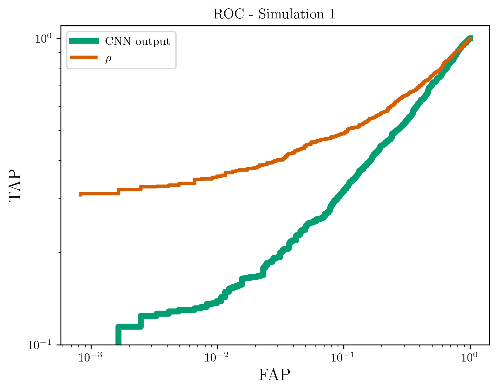
We see that the CNN statistics is less efficient in recovering signals with respect to the classical statistics $\rho$. This result is not surprising, since the Residual Network sees only an undersampled representation of the SNR time series: we recall we compressed the image into a $512\times 256$ picture which impacts the representation of the TT-SNR Map. The advantage of using such algorithms appears if we instead consider also glitches that affect the data stream, that is the case of the following sections.

VI Simulation 2

The second simulation considered in this work includes a dataset contaminated by non-Gaussian noise, which affects both the noise and injections classes. The dataset consists in 20,000 TT-SNR Maps per class, divided in training-validation and test as previously described. In this case, the injected signals include both BNS and BBH systems. The component masses for BNS and BBH injections were drawn from two different distributions. For the BNS systems, we retained a uniform distribution for the component masses as before. For BBH systems, the primary mass $m_{1}$ was sampled from an astrophysical motivated distribution [45], modeled as a power law with slope $\alpha=3.5$ and a Gaussian peak centered at $34M_{\odot}$. The secondary mass $m_{2}$ was computed via the mass ratio $q=m_{2}/m_{1}$, where $q\sim\mathcal{U}[0.15,1]$ and the final sampling followed the transformation $q=q^{0.5}$ to favor asymmetric systems. The allowed range for the primary mass was $m_{1}\in[3-200]M_{\odot}$. Both BNS and BBH signals amplitude were scaled according to the chirp-distance, defined as

$$d_{\mathrm{chirp}}=\Big(\frac{1.22}{M_{\mathrm{c}}}\Big)^{\frac{5}{6}}\cdot d$$ (11)

With $d$ is distributed according to a second-order power law, as in the previous case. This scaling accounts for the fact that the observable amplitude of a gravitational-wave signal depends on the chirp mass $M_{\mathrm{c}}$, making $d_{\mathrm{chirp}}$ a more appropriate parameter for distance-scaling when comparing signals of different masses [13]. In this simulation, we injected sine-Gaussian glitches randomly into 30$\%$ of data segments — on both injections and noise labelled — to emulate the non-Gaussian transient noise, since it is known that the matched-filtering response to such transients can extend significantly beyond the glitch time itself (see [18]). A sine-Gaussian in time domain can be written as

$$g(t)=Ae^{\big(\frac{(t-t_{0})^{2}}{\tau^{2}}\big)}cos(2\pi f_{0}t+\phi_{0})$$ (12)

In this expression, $A$ identifies the amplitude and $\tau=\frac{Q}{2\pi f_{0}}$ the duration of the pulse, where $Q$ is the dimensionless quality factor. The parameters $f_{0}$ and $t_{0}$ specify the central frequency and central time of the sine-Gaussian, respectively, while $\phi_{0}$ is the phase at $t=0$. We injected the sine-Gaussian glitches uniformly in a time window $\Delta t\in[-63,0.5]$s, taking the nominal injection time of the binary system at $t=0$. This simulates the possible effect of the glitches even when they occur well before the actual signal. The remaining sine-Gaussian parameters were sampled from uniform distributions $\mathcal{U}$, with the corresponding ranges listed in Table 1

Table 1: Parameter ranges used for the injected sine-Gaussian signals.

Parameter	Value range
Amplitude $A$	$[1\text{–}9]\times 10^{-22}$
Central frequency $f_{0}$	$[20,\,2048]~\mathrm{Hz}$
Quality factor $Q$	$[3,\,400]$
Initial phase $\phi_{0}$	$[0,\,6]$

In this simulation, we compared the CNN-assigned score $r$ with a effective statistic that incorporates the $\chi^{2}$-test as is commonly done similarly in the PyCBC pipeline to suppress glitch-induced SNR. The standard procedure involves computing the $\chi^{2}$ distribution over a specified number of frequency bins $N_{b}$, according to Eq. 5; in this case, we use $N_{b}=4$. The reweighed statistics obtained is the $\rho_{\mathrm{rw}}$ as described in Eq. 6.

We then identify the the maximum value $\rho_{\mathrm{rw}}^{\mathrm{max}}$ within the 4-seconds time window and compare it to the score $r$ for the corresponding TT-SNR Map. To evaluate and compare the classification performance of the CNN and the traditional effective statistics, we use the ROC also in this case.

We expect that the reweighted statistics $\rho_{\mathrm{rw}}^{\mathrm{max}}$, which incorporates the $\chi^{2}_{\mathrm{r}}$ test, will be significantly more effective in separating noise from signal than the raw matched-filter maximum $\rho^{\mathrm{max}}$. We then compare the ROC curves obtained using $\rho_{\mathrm{rw}}^{\mathrm{max}}$ and the CNN-output $r$ statistics to quantify the network’s ability to distinguish between glitches and true signals relative to the classical approach. Results are reported in Fig. 6(b)

(a) Simulation 2: Distribution of injected signals for $\rho_{\mathrm{opt}}$ - chirp distance $d_{\mathrm{chirp}}$ [Mpc] - CNN output

(b) Simulation 2: ROC curves for $\rho_{\mathrm{rw}}^{\mathrm{max}}$, $r$ and $\rho^{\mathrm{max}}$ statistics.

Figure 6: Results for BBH and BNS signals injected in Gaussian noise polluted with sine-Gaussian glitches.

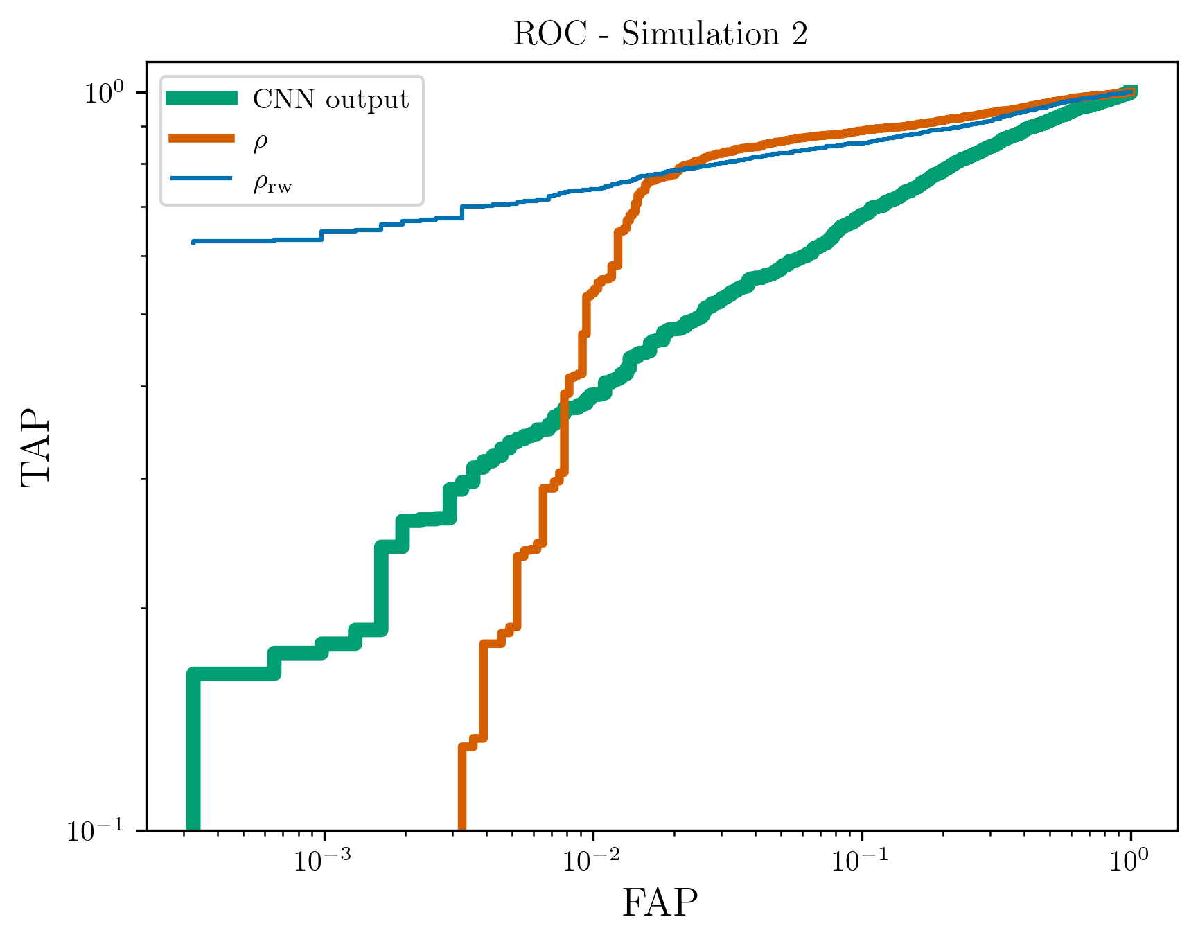
In the results we observe that the CNN output outperforms the raw matched-filter statistic $\rho$ statistics for low false alarm probabilities. However, the reweighted statistic $\rho_{\mathrm{rw}}^{\mathrm{max}}$ remains the most effective overall. Furthermore, we see that the network fails to assign high score to nearby signal (Fig. 6(a)), a behavior can suggests underfitting issues, since relatively few samples fall in that specific interval.

VII Simulation 3

In this study, we included additional physical information in the injected signals that is not represented in the template bank. Specifically, spin effects were incorporated by assigning aligned-spin components drawn from uniform distributions. For neutron stars, we used a conservative spin range of $\chi^{1,2}_{z,NS}\in\mathcal{U}[-0.5,0.5]$, while for black holes we adopted $\chi^{1,2}_{z,BH}\in\mathcal{U}[-0.9,0.9]$, reflecting the typically higher spin magnitudes of BH [65]. As in the previous studies, the dataset was divided into training-validation-test in a $70-15-15$ split. However, the total dataset size was significantly larger, consisting in 40,000 TT-SNR Maps per class for both noise and injection samples. The relatively smallness of the network allowed a training time around $\sim 140$ minutes. The performance comparison followed the same procedure as in the previous section, and is represented in Fig. 7(b).

(a) Simulation 3: Distribution of injected signals for $\rho_{\mathrm{opt}}$ - chirp distance $d_{\mathrm{chirp}}$ [Mpc] - CNN output

(b) Simulation 3: ROC curves for $\rho_{\mathrm{rw}}^{\mathrm{max}}$, $r$ and $\rho^{\mathrm{max}}$ statistics.

Figure 7: Results for BBH and BNS signals encoding spin parameters and injected in Gaussian noise polluted with sine-Gaussian glitches.

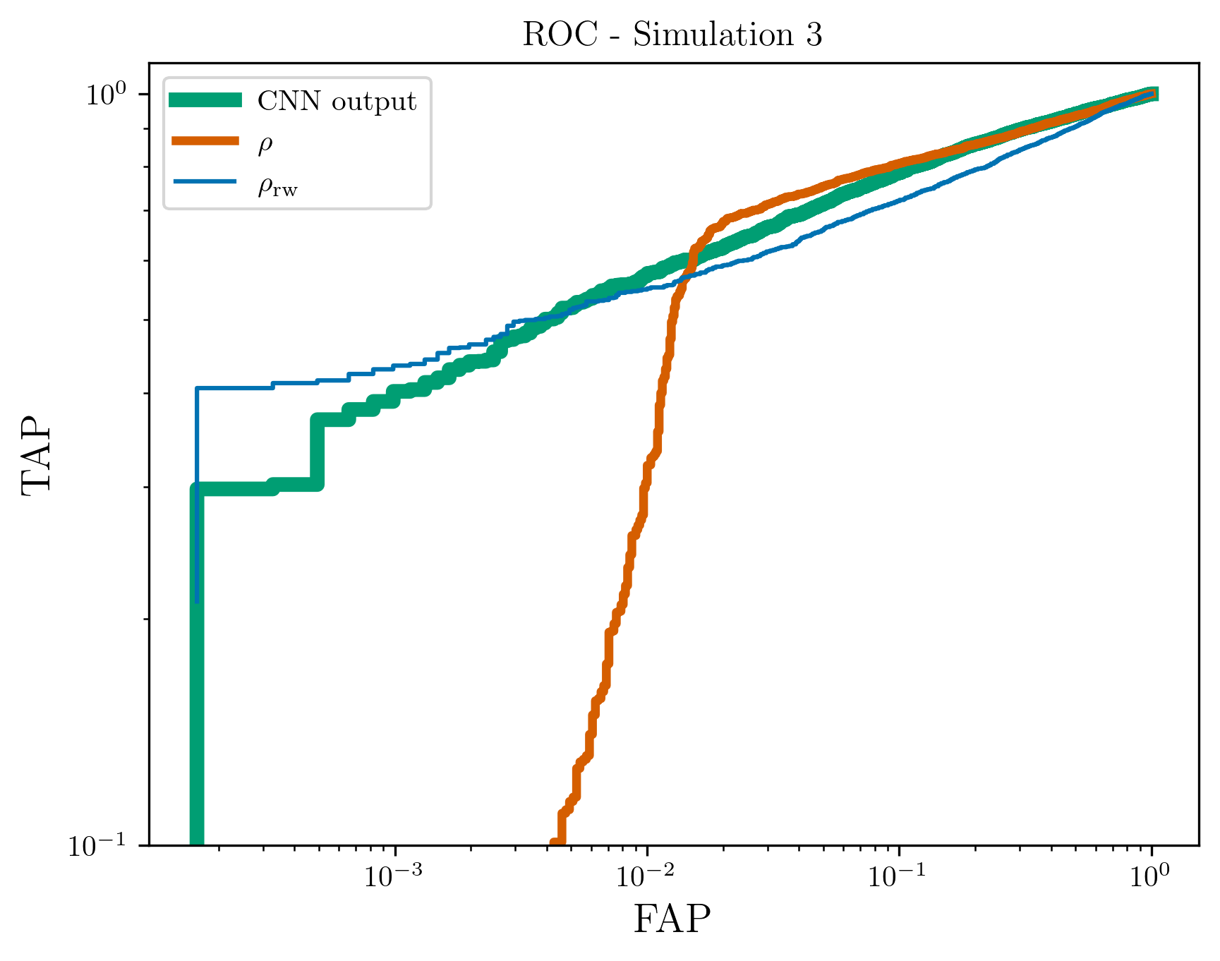
In this case the physical effect of spin-absence from the template bank causes the $\chi^{2}$-test to down-rank the SNR associated with the true injections. In contrast, EasyResNet is not affected by this mismatch and achieves performance comparable to that of the matched-filtering search, even in presence of spin. Regarding the chirp-distance distribution (Fig. 7(a)), we see that the issue affecting the nearby (and loudest) signals is no more present. Since here we used twice the amount of data, it is reasonable to assert that the network has learned well enough to generalize the shape of the signal in the whole distance range.

VIII Simulation 4

In this final simulation, we extend the investigation of the capability of the TT-SNR MAP to encode physical information that goes beyond the physics explicitly included in the template bank used to construct the map itself. In particular, we expect this representation to capture not only the presence of a signal, but also the specific physical effect characterizing the injected waveform. Moreover, motivated by the encouraging results obtained in the previous section, we anticipate that a network trained on these TT-SNR MAP will achieve performance comparable to — or potentially exceeding — that of the classical $\rho_{\mathrm{rw}}$ method. To this end, we considered five different families of signal injections, each characterized by a different physical effect or scenario that the TT-SNR MAP is expected to represent and that the network is trained to distinguish. In this study we deliberately focus on isolating the impact of individual physical effects rather than reproducing their expected astrophysical distributions. Consequently, we adopt non-physical distributions for these effects, which nevertheless suffice for the exploratory nature of this analysis. Finally, to assess whether the network is capable of detecting signals that include physical features not represented in the template bank, we inject signals at relatively small distances, resulting in optimal signal-to-noise ratios significantly higher than in the previous cases. This choice allows us to restrict the analysis to scenarios in which the presence of a signal is unambiguous, thereby isolating the network’s ability to recognize signals with additional physical content rather than its sensitivity near the detection threshold.

First, we consider an extreme version of the scenario described in Simulation 3 campaign, restricting the spin configurations to purely align or anti-align cases with respect to the orbital angular momentum. Specifically, we adopt extremal spin values for the BNS ($\chi^{z}_{1,2}=\pm 0.5$) and for the BBH ($\chi^{z}_{1,2}=\pm 1$) population. The mass distributions of injected signals are identical to those used in the Simulation 3 campaign.

The second family of simulations consists of superimposed signal injections. This scenario is of particular interest in the context of the future 3G detectors such as Einstein Telescope [2] and Cosmic Explorer [22] . Owing to their increased sensitivity and extended low-frequency coverage, these instruments are expected to observe a high rate of loud signals, which will likely overlap in the detector strain data. Analyzing such data streams poses significant challenges, and the method explored here may provide a valuable approach in this direction [63]. In this study, we consider only BNS signals with component masses and spins drawn from uniform distributions: $m_{1,2}\sim\mathcal{U}(1.4,3)M_{\odot}$; $\chi^{z}_{1,2}\sim\mathcal{U}(-0.5,0.5)$. For simplicity, we inject only two signals per realization, separated by a short temporal delay uniformly distributed in the interval $[-0.02,0.02]$ s. The second injection is constructed to have component masses close to the first signal, in order to mimic the most challenging case of highly similar overlapping events. Specifically, the masses of the second signal are defined as $m^{\prime}_{1,2}=m_{1,2}+\mathcal{U}(-0.02,0.02)M_{\odot}$. A representative example of such superimposed injections is shown in Fig. 8(a) and Fig. 8(b).

(a) BNS non-spinning ($1.4-1.4\,M_{\odot}$) superimposed signals. The TT-SNR MAP clearly encodes the presence of two signals that are closely separated in time and nearly identical in parameter space. An interference-like pattern emerges from the superposition of the signal representations produced by the template-based SNR time series, highlighting the TT-SNR MAP’s ability to capture overlapping events.

(b) BNS non-spinning ($1.4-1.4\,M_{\odot}$) superimposed signals, zoomed view around the merging time.

Figure 8: TT-SNR-map resulting from injected BNS non-spinning superimposed signals

The following injection campaign incorporates the presence of high-order modes (HMs) [75] in the injected signals (see Fig. 9). This case is particularly relevant because high-order modes encode a more accurate description of the gravitational waveform, arising from additional contributions in the spherical-harmonic decomposition of the solution to the Einstein Equations. To maximize the impact of HMs on the observed waveform, all the signals are injected with an inclination angle $\iota=\frac{\pi}{2}$, corresponding to an edge-on orientation of the binary system. In this campaign, we consider non-spinning BNS and BBH system, with component masses drawn from the same uniform and power-law distributions adopted for the two populations in the previous simulations. The waveforms are generated using the SEOBNRv4HM approximant [59].

Figure 9: Example of a BNS ($1.4-1.4M_{\odot}$) waveform including higher-order modes, injected with inclination $\iota=\frac{\pi}{2}$. The TT-SNR MAP shows a clear modification of the central region, where the sharp rectangular features typically present in the standard representation are smoothed out by the contribution of higher-order modes. A similar structure is also visible at lower amplitudes, repeating regularly at later times.

The fourth family of injections investigated the impact of spin-induced precession on the TT-SNR MAP. Precessing signals are of particular interest because they encode rich information about the properties of the compact binaries, including the orbital geometry and characteristic length scales of the system [24, 25]. Moreover, precession provides key insight into the spin distribution of BBH population, thereby constraining their possible formation channels [33, 47]. In this campaign, we considered a population of signals equally divided among BNS, neutron-star black-hole (NSBH) and BBH systems. The mass distributions for the BNS and BBH populations follow those adopted in the previous simulations. For the NSBH systems, the component masses are distributed as $m_{1}\sim\mathrm{U}(1.4,3)M_{\odot}$ and $m_{2}\sim\mathrm{U}(10,25)M_{\odot}$. For all the three populations, the spin components are configured to induce strong precession by drawing the in-plane components from uniform distributions, $\chi^{x}_{1,2},\chi^{y}_{1,2}\sim\mathrm{U}(0.4,0.5)$, while setting the aligned component to zero, $\chi^{z}_{1,2}=0$. As in the previous injection families, the inclination angle is fixed to $\iota=\frac{\pi}{2}$ to enhance the precessional effects. Only the dominant quadrupole mode $(\ell,m)=(2,2)$ is retained in this analysis. The approximant used is SEOBNRv5PHM [62]. An example of precessing signal in this configuration is shown in Fig. 10.

Figure 10: TT-SNR MAP of precessing NSBH system ($1.4-25M_{\odot}$) injected with inclination $\iota=\frac{\pi}{2}$. The effect of spin-induced precession manifests as a modulation of the TT-SNR MAP structure, producing beam-like features radiating from the center of the map. These patterns reflect the time-dependent orbital-plane precession imprinted on the signal morphology.

The final injection campaign explores the impact of orbital eccentricity on the TT-SNR MAP representation. Eccentric gravitational-wave signals are of particular interest because they provide valuable clues about the formation channels of compact binaries, especially in dynamical environments such as globular clusters or galactic nuclei, where binaries may retain significant eccentricity when entering the detector sensitivity band [57, 58].

This study considers non-spinning BNS and BBH signals. For the two populations, the orbital eccentricity is drawn from uniform distributions with relatively high values, chosen to enhance the imprint of eccentricity on the waveform morphology: $e_{\mathrm{BNS}}\sim\mathcal{U}(0.4,0.6)$ and $e_{\mathrm{BBH}}\sim\mathcal{U}(0.3,0.5)$. Such values are intentionally higher than those expected for the majority of astrophysical sources detectable by current instruments, but they are well suited for this exploratory study aimed at testing the network’s sensitivity to eccentric features that are not encoded in the template bank. Waveforms are generated using SEOBNRv5E_td approximant [26]. A representative example of an eccentric injection from this campaign is shown in see Fig. 11.

Figure 11: Representative example illustrating the effect of eccentricity in the TT-SNR MAP. Here it is shown a $1.4-6M_{\odot}$ non spinning system with $e=0.3$, chosen outside the injection families for illustrative purposes. The imprint of eccentricity is clearly visible as a repeating structure beneath the main TT-SNR MAP pattern, appearing twice and introducing distinctive features associated with the non-circular orbital dynamics.

For all injection families, $30\%$ of the signals are contaminated with sine-Gaussian glitches. Each family also consists in $8,000$ injections, resulting in a total of $40,000$ TT-SNR MAP images labelled as injection. Following the same methodology adopted in the previous simulation campaigns, we construct a balanced dataset by including an additional $40,000$ noise-labelled TT-SNR MAPs, generated from Gaussian noise and contaminated with the same ratio of sine-Gaussian glitches at the same relative rate. The full dataset is then split into training, validation and test subsets using the same proportions adopted for the previous populations $(70\%-15\%-15\%)$. The trained network is subsequently evaluated compared again classical detection statistics through the ROC curves. Owing to the network’s rapid convergence and strong learning capability, the number of training epochs is reduced to five, beyond which no statistically significant performance improvements are observed. The corresponding results are shown in 12.

Figure 12: Results of the ROC curves for the 5 families injected signals campaign encoding physics not included in the template bank used to construct the TT-SNR Map. The signals are injected in Gaussian noise polluted with sine-Gaussian glitches.

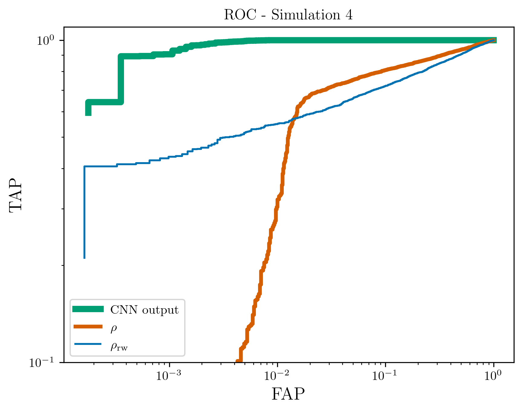
In this study-case, the network exhibits an improved capability to discriminate between noise and signal with respect to the previous simulation campaigns. The ROC curves obtained with the ResNet architecture consistently lie above those associated with both the $\rho$ and $\rho_{\mathrm{rw}}$ statistics, indicating a systematic gain in detection performance. This behavior is not unexpected, as the injected signals are placed at relatively small distances, leading to TT-SNR MAPs that clearly encode the presence of signal and its associated physical features. Moreover, the increase in performance can be partially attributed to the larger size of the training dataset, which is twice that used in the S-3 campaign. The absolute number of training samples is a well-known factor affecting the stability and generalization capability of deep neural networks, and its increase contributes to the robust behavior observed in this case.

IX Conclusions

In this proof-of-concept study, we trained and tested a Convolutional Neural Network (EasyResNet) on TT-SNR Maps constructed from matched-filtering SNR time series. Four successive simulation campaigns were performed. The first used injections drawn from a well-defined parameter space embedded in purely Gaussian noise. The second introduced sine-Gaussian glitches into the background and extended the injections to include BBH systems. The third and fourth incorporated physical effects — aligned component spins, high-order-modes, precession, eccentricity and overlapping signals — not represented at all in the template bank, in order to test network’s robustness relative to a matched filtering analysis.

EasyResNet consistently learned the TT-SNR-Map patterns associated with the true signals and distinguished them from noise. This advantage was most pronounced when the injected signals contained physical parameters not covered by the bank, a regime in which the classical matched-filter ranking is degraded. An advantage of this method is that the $\chi^{2}$ veto is not needed to be computed for rejecting the glitches, since the network can learn automatically how signals and spurious noise behave in the TT-SNR-Map. This comes with fast inference — $\sim 3$ ms per image using only off-the-shelf CPUs without particular optimizations — making the method attractive for low-latency applications.

Since in this work the search is performed solely in terms of the chirp mass $M_{\mathrm{c}}$, the resulting template bank is consistently reduced in size. Further studies are therefore required to confirm the detection sensitivity of the network relative to state-of-the-art CBC search pipelines that exploit full-sized template bank. If confirmed, this approach could offer a viable alternative for third-generation detectors such as the Einstein Telescope: a TT-SNR-Map-based analysis combined with a trained Network could produce triggers using a significantly reduced template bank.

In this work, these results were obtained using standard CPU resources, without exploiting GPU-based parallelization for network training. This limitation necessitated the adoption of under-sampled TT-SNR-map representations, which negatively impacted the network’s capabilities and overall performance. Access to greater computational resources in future studies is expected to enable more efficient architectures, as the algorithm would be able to exploit the full information content of the SNR time series rather than a down-sampled representation.

Future work will focus on enlarging EasyResNet to exploit deeper architectures and benchmarking against production-level LVK search pipelines to quantify gains in detection efficiency and computational cost.

Appendix A Correlation between the templates

The matched-filtering analysis consists in correlating the detector’s output $s(t)$ with the templates $h(t)$, listed in the template bank, and weighting the correlation by the detector’s noise power spectral density $S_{n}(f)$. The output of the matched-filtering is the signal-to-noise-ratio time series $\rho(t)$, and this quantity shows a peak in correspondence to the merging time if the template and the signal are similar enough. The $\rho(t)$ of each template will encode the physical difference between the template and the signal present in data. An efficient way to visualize it is to consider the spectrogram of a reference signal, with chirp mass $M_{\mathrm{c}}^{\mathrm{ref}}=2.17M_{\odot}$ merging at $t_{\mathrm{ref}}=40$s and see how templates with chirp mass below and above act differently when compared with the reference one. For instance, suppose that a template with $M_{\mathrm{c}}^{1}=0.95M_{\odot}$ merges at $t_{1}=38$s, and then the same template merges at $t_{2}=42$s. In Fig. 13(a) we see that the template will cross the signal if it merges after the reference time. On the other side (Fig. 13(b)), considering instead a template with $M_{\mathrm{c}}^{2}=4.35M_{\odot}$, this time the behavior will be the opposite, and the template will cross the reference if it merges before the $t_{\mathrm{ref}}$. This phenomenological description describe qualitatively why we expect structures as those showed in Fig. 1.

(a) Spectrogram of systems with $M_{\mathrm{c}}^{1}=0.95\,M_{\odot}$ merging time at $t_{1}=38\,\mathrm{s}$ (red line), $M_{\mathrm{c}}^{\mathrm{ref}}$ time at $t_{0}=40\,\mathrm{s}$ (green line), and $M_{\mathrm{c}}^{1}=0.95\,M_{\odot}$ merging time at $t_{2}=42\,\mathrm{s}$ (blue line).

(b) Spectrogram of systems with $M_{\mathrm{c}}^{2}=4.35\,M_{\odot}$ merging time at $t_{1}=38\,\mathrm{s}$ (red line), $M_{\mathrm{c}}^{\mathrm{ref}}$ time at $t_{0}=40\,\mathrm{s}$ (green line), and $M_{\mathrm{c}}^{2}=4.35\,M_{\odot}$ merging time at $t_{2}=42\,\mathrm{s}$ (blue line).

References

- [1] (2015) Advanced ligo. Class. Quantum Grav. 32, pp. 074001. External Links: 1411.4547 Cited by: §I.
- [2] (2025) The science of the einstein telescope. Note: arXiv:2503.12263 External Links: 2503.12263 Cited by: §I, §VIII.
- [3] (2025) GWTC-4.0: An Introduction to Version 4.0 of the Gravitational-Wave Transient Catalog. External Links: Link Cited by: §III.
- [4] (2016-06) GW150914: first results from the search for binary black hole coalescence with advanced ligo. Physical Review D 93 (12). External Links: ISSN 2470-0029, Link, Document Cited by: §II.
- [5] (2016) Observation of gravitational waves from a binary black hole merger. Phys. Rev. D 93, pp. 122003. External Links: 1602.03839 Cited by: §I.
- [6] (2019) GWTC-1: a gravitational-wave transient catalog of compact binary mergers. Phys. Rev. X 9, pp. 031040. External Links: 1811.12907 Cited by: §I.
- [7] (2021) GWTC-2: compact binary coalescences observed by ligo and virgo during the first half of the third observing run. Phys. Rev. X 11, pp. 021053. External Links: 2010.14527 Cited by: §I.
- [8] (2021) GWTC-2.1: deep extended catalog of compact binary mergers observed by ligo and virgo during o3a. Phys. Rev. D. Note: arXiv:2108.01045 External Links: 2108.01045 Cited by: §I.
- [9] (2021) GWTC-3: compact binary coalescences observed by ligo and virgo during the second part of the third observing run. Note: arXiv:2111.03606 External Links: 2111.03606 Cited by: §I.
- [10] (2015) Advanced virgo: a second-generation interferometric gravitational wave detector. Class. Quantum Grav. 32, pp. 024001. External Links: 1408.3978 Cited by: §I.
- [11] (2020) Overview of kagra: kagra science. Prog. Theor. Exp. Phys. 2021, pp. 05A103. External Links: Document, 2008.02921 Cited by: §I.
- [12] (2005) Time-frequency discriminator for gravitational wave detection. Phys. Rev. D 71, pp. 062001. External Links: Document, gr-qc/0405045 Cited by: §II.
- [13] (2012) FINDCHIRP: an algorithm for detection of gravitational waves from inspiraling compact binaries. Physical Review D 85, pp. 122006. External Links: Document Cited by: §VI.
- [14] (2025) The mbta pipeline for detecting compact binary coalescences in the fourth ligo-virgo-kagra observing run. Class. Quantum Grav. 42, pp. 105009. External Links: 2501.04598 Cited by: §I.
- [15] (2019) LISA pathfinder: mission overview. Note: arXiv:1903.08924 External Links: 1903.08924 Cited by: §I.
- [16] (2013-01) Searching for gravitational waves from binary coalescence. Phys. Rev. D 87, pp. 024033. External Links: Document, Link Cited by: §II.
- [17] (2012) Detecting spins in binary neutron star inspirals. Phys. Rev. D 86, pp. 084017. External Links: Document, 1207.6406 Cited by: §II.
- [18] (2014) Sine-gaussian glitches in gravitational-wave detectors. Class. Quantum Grav. 31, pp. 015016. External Links: Document, 1304.0008 Cited by: §VI.
- [19] (2021) Real-time search for compact binary mergers in advanced LIGO and Virgo’s third observing run using PyCBC live. APJ 923, pp. 254. Cited by: §I.
- [20] (2017-11) A unified approach to <mml:math xmlns:mml="http://www.w3.org/1998/math/mathml" display="inline"><mml:msup><mml:mi>χ</mml:mi><mml:mn>2</mml:mn></mml:msup></mml:math> discriminators for searches of gravitational waves from compact binary coalescences. Physical Review D 96 (10). External Links: ISSN 2470-0029, Link, Document Cited by: §II.
- [21] (2025) LISA: laser interferometer space antenna. Note: NASA/ESAAccessed June 2025 External Links: Link Cited by: §I.
- [22] (2021) A horizon study for cosmic explorer: science, observatories, and community. Note: arXiv:2109.09882 External Links: 2109.09882 Cited by: §I, §VIII.
- [23] (2024-02) Performance of the low-latency gstlal inspiral search towards ligo, virgo, and kagra’s fourth observing run. Physical Review D 109, pp. 042008. External Links: Document, Link Cited by: §I.
- [24] (2018-02) Using spin to understand the formation of ligo and virgo’s black holes. The Astrophysical Journal Letters 854 (1), pp. L9. External Links: ISSN 2041-8213, Link, Document Cited by: §VIII.
- [25] (2017-08) Distinguishing spin-aligned and isotropic black hole populations with gravitational waves. Nature 548 (7668), pp. 426–429. External Links: ISSN 1476-4687, Link, Document Cited by: §VIII.
- [26] (2025-08) Accurate waveforms for eccentric, aligned-spin binary black holes: the multipolar effective-one-body model seobnrv5ehm. Physical Review D 112 (4). External Links: ISSN 2470-0029, Link, Document Cited by: §VIII.
- [27] (2008) SEARCHING for gravitational waves from binary systems in non-stationary data. Ph.D. Thesis, Louisiana State University. Cited by: §II.
- [28] (2014) Investigating the effect of precession on compact binary coalescence detection. Phys. Rev. D 89, pp. 024010. External Links: Document Cited by: §II.
- [29] (2015) Deep residual learning for image recognition. Note: arXiv:1512.03385 External Links: 1512.03385 Cited by: §IV.
- [30] (1968) Statistical theory of signal detection. 2 edition, Pergamon Press, London. Cited by: §II, §II.
- [31] (2012-07) Summed parallel infinite impulse response filters for low-latency detection of chirping gravitational waves. Phys. Rev. D 86, pp. 024012. External Links: Document, Link Cited by: §I.
- [32] (2015-07–09 Jul) Batch normalization: accelerating deep network training by reducing internal covariate shift. In Proceedings of the 32nd International Conference on Machine Learning, F. Bach and D. Blei (Eds.), Proceedings of Machine Learning Research, Vol. 37, Lille, France, pp. 448–456. External Links: Link Cited by: §IV.
- [33] (2022-07) Inferring spin tilts at formation from gravitational wave observations of binary black holes: interfacing precession-averaged and orbit-averaged spin evolution. Physical Review D 106 (2). External Links: ISSN 2470-0029, Link, Document Cited by: §VIII.
- [34] (2024) Efficient stochastic template bank using inner product inequalities. Note: arXiv:2407.03406 External Links: 2407.03406 Cited by: §II.
- [35] (2014) Adam: a method for stochastic optimization. CoRR abs/1412.6980. External Links: Link Cited by: §IV.
- [36] (2005-12) Constraint likelihood analysis for a network of gravitational wave detectors. Phys. Rev. D 72, pp. 122002. External Links: Document, Link Cited by: §I.
- [37] (2016-02) Method for detection and reconstruction of gravitational wave transients with networks of advanced detectors. Phys. Rev. D 93, pp. 042004. External Links: Document, Link Cited by: §I.
- [38] (2012) ImageNet classification with deep convolutional neural networks. In Advances in Neural Information Processing Systems, Cited by: §IV.
- [39] (2015) Deep learning. Nature 521, pp. 436–444. External Links: Document Cited by: §IV.
- [40] (2023) LIGO-india: a planned joint india–us detector. Note: LIGO Laboratory, Caltech/MITAccessed June 2025 External Links: Link Cited by: §I.
- [41] (2025) GWTC-4.0: updating the gravitational-wave transient catalog with observations from the first part of the fourth ligo-virgo-kagra observing run. Note: arXiv:2508.18082 External Links: 2508.18082 Cited by: §I.
- [42] (2017) GW170817: observation of gravitational waves from a binary neutron star inspiral. Phys. Rev. Lett. 119, pp. 161101. External Links: 1710.05832 Cited by: §I.
- [43] (2020) GW190521: a binary black hole merger with a total mass of 150 solar masses. Phys. Rev. Lett. 125, pp. 101102. External Links: 2009.01075 Cited by: §I.
- [44] (2020) Properties and astrophysical implications of the binary black hole merger gw190521. Astrophys. J. Lett. 900, pp. L13. External Links: 2009.01190 Cited by: §I.
- [45] (2021) Population properties of compact object mergers observed by ligo and virgo during the third observing run. Phys. Rev. X 13, pp. 011048. External Links: 2111.03634 Cited by: §VI.
- [46] (2014) Network in network. In International Conference on Learning Representations (ICLR), Cited by: §IV.
- [47] (2021) Formation channels of single and binary stellar-mass black holes. In Handbook of Gravitational Wave Astronomy, pp. 1–65. External Links: ISBN 9789811547027, Link, Document Cited by: §VIII.
- [48] (2024) A machine-learning pipeline for real-time detection of gravitational waves from compact binary coalescences. Note: arXiv:2403.18661 External Links: 2403.18661 Cited by: §I.
- [49] (2025) Binary neutron star detection with a deep learning pipeline. Phys. Rev. D 111, pp. 024035. External Links: 2409.06266 Cited by: §I.
- [50] (2017-02) Analysis framework for the prompt discovery of compact binary mergers in gravitational-wave data. Physical Review D 95 (4). External Links: ISSN 2470-0029, Link, Document Cited by: §II.
- [51] (2017-02) Analysis framework for the prompt discovery of compact binary mergers in gravitational-wave data. Phys. Rev. D 95, pp. 042001. External Links: Document, Link Cited by: §I, §II.
- [52] (2024) Gwastro/pycbc: v2.3.3 release of pycbc. External Links: Document, Link Cited by: §III.
- [53] (2022) Deep residual networks for gravitational wave detection. Note: arXiv:2211.01520 External Links: 2211.01520 Cited by: §I.
- [54] (2015) An introduction to convolutional neural networks. CoRR abs/1511.08458. External Links: 1511.08458 Cited by: §III.
- [55] (2020) Multipolar effective-one-body waveforms for precessing binary black holes: construction and validation. Physical Review D 102, pp. 044055. External Links: Document Cited by: §III.
- [56] (1996) Search templates for gravitational waves from inspiraling binaries: choice of template spacing. Phys. Rev. D 53, pp. 6749. External Links: Document, gr-qc/9511032 Cited by: §III.
- [57] (1963-07) Gravitational radiation from point masses in a keplerian orbit. Phys. Rev. 131, pp. 435–440. External Links: Document, Link Cited by: §VIII.
- [58] (1964-11) Gravitational radiation and the motion of two point masses. Phys. Rev. 136, pp. B1224–B1232. External Links: Document, Link Cited by: §VIII.
- [59] (2023-12) Laying the foundation of the effective-one-body waveform models seobnrv5: improved accuracy and efficiency for spinning nonprecessing binary black holes. Physical Review D 108 (12). External Links: ISSN 2470-0029, Link, Document Cited by: §VIII.
- [60] (2016) Frequency domain reduced order model of aligned-spin effective-one-body waveforms with generic mass ratios and spins. Physical Review D 93 (6), pp. 064041. External Links: Document Cited by: §III.
- [61] (2023) SEOBNRv5PHM: next generation of accurate and efficient multipolar precessing-spin effective-one-body waveforms for binary black holes. Note: arXiv:2303.18046 External Links: 2303.18046 Cited by: §III.
- [62] (2023) SEOBNRv5PHM: next generation of accurate and efficient multipolar precessing-spin effective-one-body waveforms for binary black holes. External Links: 2303.18046, Link Cited by: §VIII.
- [63] (2022-11) Addressing the challenges of detecting time-overlapping compact binary coalescences. Phys. Rev. D 106, pp. 104045. External Links: Document, Link Cited by: §VIII.
- [64] (1958) The perceptron: a probabilistic model for information storage and organization in the brain. Psychological Review 65, pp. 386–408. External Links: Document Cited by: §IV.
- [65] (2019) Binary black hole population properties inferred from the first and second observing runs of advanced ligo and advanced virgo. Monthly Notices of the Royal Astronomical Society 484, pp. 4216–4229. External Links: Document Cited by: §VII.
- [66] (2019) Template banks for compact binary coalescences. Phys. Rev. D 99, pp. 024048. External Links: Document, 1711.08743 Cited by: §II.
- [67] (1986) Learning representations by back-propagating errors. Nature 323 (6088), pp. 533–536. External Links: Document Cited by: §IV.
- [68] (2019) The gstlal search analysis methods for compact binary mergers in advanced ligo’s second and advanced virgo’s first observing runs. External Links: 1901.08580, Link Cited by: §I.
- [69] (2022) MLGWSC-1: the first machine learning gravitational-wave search mock data challenge. Note: arXiv:2209.11146 External Links: 2209.11146 Cited by: §I.
- [70] (2009) Advanced ligo anticipated sensitivity curves. Technical report Technical Report LIGO-T0900288, LIGO Scientific Collaboration. External Links: Link Cited by: §III.
- [71] (2024) Real-time detection of unmodelled gravitational-wave transients using convolutional neural networks. Note: arXiv:2009.14611 External Links: 2009.14611 Cited by: §I.
- [72] (2025) GWTC-4.0: Methods for Identifying and Characterizing Gravitational-wave Transients. arXiv e-prints. External Links: Link Cited by: §III.
- [73] (2023-08) Improved ranking statistics of the gstlal inspiral search for compact binary coalescences. Phys. Rev. D 108, pp. 043004. External Links: Document, Link Cited by: §I.
- [74] (2016) The pycbc search for gravitational waves from compact binary coalescence. Class. Quantum Grav. 33, pp. 215004. External Links: 1508.02357 Cited by: §II.
- [75] (2017) Effects of nonquadrupole modes in the detection and parameter estimation of black hole binaries with nonprecessing spins. Physical Review D 96, pp. 124024. External Links: Document Cited by: §VIII.
- [76] (2025) Hybrid algorithm combining matched filtering and convolutional neural networks for searching gravitational waves from binary black hole mergers. External Links: 2512.12399, Link Cited by: §I.