A finite element continuous data assimilation framework for a Navier–Stokes–Cahn–Hilliard system

Abstract.

This paper studies a coupled two-dimensional Navier–Stokes–Cahn–Hilliard phase-field model augmented by a transported auxiliary field, and develops a continuous data assimilation (CDA) framework for recovering its trajectories from coarse-in-space observations.

We formulate a nudging-based CDA system for the coupled NSCH–auxiliary-field model, in which coarse measurements are incorporated through a general linear observation operator. The observation mechanism is described abstractly by an interpolant satisfying an $H^{2}$-type approximation property, which is compatible with coarse spatial observations obtained from mesh coarsening and reconstruction.

At the continuous level, we record two structural properties of the model: a formal energy law for the reference system and an evolution law for the phase mean in the assimilated dynamics. At the discrete level, we introduce a capped fully discrete finite element splitting scheme using continuous quadratic elements for the phase, chemical potential, velocity, and auxiliary field, together with continuous linear elements for the pressure. For this scheme, we prove one-step well-posedness and establish a stepwise a priori estimate for the capped method.

Numerical experiments illustrate the practical behavior of the proposed CDA approach. They demonstrate recovery from strongly mismatched initial conditions and show how synchronization depends on the observation resolution, boundary forcing, and feedback strength. A coarse-indistinguishability experiment further shows that identical coarse initial information may correspond to distinct fine-scale evolutions, while the assimilated dynamics select the trajectory determined by the supplied time-dependent observations.

Keywords. Navier–Stokes–Cahn–Hilliard $\cdot$ Continuous data assimilation $\cdot$ Nudging $\cdot$ Finite element method $\cdot$ Phase-field models

MSC 2010. 35Q35, 35K55, 35K57, 65M60, 93C20.

1. Introduction

Phase-field models provide a flexible framework for describing multiphase hydrodynamics in which interfaces are represented by thin transition layers rather than sharp boundaries. The underlying diffuse-interface viewpoint goes back to the classical work of Cahn and Hilliard on interfacial free energy, and has since become a standard modeling tool for interfacial fluid phenomena; see, for example, [8, 5]. Within this paradigm, the Navier–Stokes–Cahn–Hilliard (NSCH) system, often referred to as Model H and its variants, provides a diffuse-interface description of incompressible two-phase flow that couples hydrodynamics with interfacial mixing and capillarity. Because the interface is represented through an order parameter rather than tracked explicitly, phase-field formulations are especially effective in situations involving topological changes, such as droplet merger and breakup, without the need for front tracking. Representative examples include microfluidic droplet formation and breakup [7]. In biomechanics and hemodynamics, phase-field methods have also been used to describe thrombus formation and remodeling in flowing blood, incorporating spatially varying material properties and permeability within a unified energetic framework [50, 47, 46]. Related developments connect phase-field hydrodynamics to complex-fluid effects such as viscoelasticity and transported microstructure; see, for example, [35, 25].

From the analytical viewpoint, the NSCH system and related diffuse-interface models have been studied extensively. For two-phase flows with matched densities, diffuse-interface models coupled to incompressible Navier–Stokes equations were analyzed by Abels [4], while for the variable-density setting strong and weak solvability results were established by Abels and collaborators [3, 1]. Degenerate-mobility variants have also been investigated, with the physically important feature that the order parameter remains in the admissible interval under suitable assumptions [2]. For the NSCH system itself, uniqueness and regularity theory with physically relevant potentials has been developed in several settings, including strong well-posedness in two dimensions and local strong theory in three dimensions [26]. Long-time dynamics for CHNS-type systems have likewise been studied through attractors and asymptotic behavior [22, 27]. Broader background on the Cahn–Hilliard equation and its variants may be found in the surveys and monographs [37, 38]. Other works incorporate additional physical couplings and nonlinear effects, such as thermo-induced Marangoni forcing [45] and chemotaxis-driven or singular-potential regimes in two dimensions [31]. Motivated in part by thrombus modeling, rigorous PDE analyses have also been obtained for phase-field blood–thrombus systems, including local strong well-posedness results in three dimensions [33] and in two dimensions [29]. These studies provide a useful foundation for investigating algorithmic questions in situations where only partial information about the evolving state is available.

On the numerical side, the CHNS system has generated a substantial literature devoted to efficient and stable discretizations. Among widely used approaches are convex-splitting and pressure-projection methods, decoupled energy-stable schemes, adaptive energy-stable methods, and second-order linear schemes that preserve discrete energy dissipation; see, for instance, [30, 40, 13, 10, 49]. Such works show that preserving as much as possible of the energetic structure of the continuous model is central to robust computation. They also highlight the practical role of splitting, decoupling, and linearization in making phase-field fluid solvers computationally feasible. These considerations are particularly relevant in the present setting, where the coupled NSCH dynamics are further enriched by a transported auxiliary field and by assimilation terms driven by coarse observations.

A central practical difficulty is that accurate initial conditions and complete state observations are rarely accessible in applications. Data assimilation addresses this issue by incorporating observations into the model dynamics in order to recover, or track, the underlying trajectory. Among continuous-in-time approaches, the nudging framework of Azouani–Olson–Titi (AOT) has attracted considerable attention because of its relative simplicity at the PDE level and its connection with the idea that dissipative systems possess finitely many determining parameters [32, 6]. A growing literature studies continuous and discrete data assimilation for fluid models, including computational validation for the two-dimensional Navier–Stokes equations [24], discrete-in-time assimilation for the same system [21], analytical results for convection models under partial observations [18], and abridged or approximate assimilation procedures using reduced sets of measurements or regularized models [17, 34]. For phase-field dynamics, CDA-type ideas have also been explored for the Cahn–Hilliard equation itself [15]. More directly relevant to the present work, CDA has been developed for the two-dimensional Cahn–Hilliard–Navier–Stokes system, where convergence to the reference trajectory can be established under suitable resolution and nudging conditions [48]. On the numerical side, data-assimilation modifications of NSCH have also been coupled with energy-stable time discretizations driven by coarse observed data [41]. At the same time, recent work has emphasized that nudging-type recovery may fail in non-dissipative regimes where determining parameters do not exist, underscoring the importance of dissipativity and observability in the underlying model [44].

The purpose of the present paper is to formulate and study a continuous data assimilation framework for a coupled NSCH-type phase-field model augmented by a transported auxiliary field. The additional field is intended to represent transported microstructural information and contributes an extra stress term in the momentum balance, making the system a natural extension of NSCH models arising in complex-fluid and thrombus-inspired settings [35, 50, 33, 29, 25]. We restrict attention to two spatial dimensions and focus on the formulation of the CDA model, its basic structural properties, a practical capped fully discrete finite element realization, and the resulting computational behavior.

More precisely, we first introduce the coupled NSCH–$\psi$ system and the associated nudging-based CDA dynamics driven by coarse-in-space observations through a general linear observation operator. We then record two basic structural properties of the continuous system: a formal energy law for the reference dynamics and an evolution law for the phase mean in the assimilated system. The observation mechanism is described abstractly through an interpolant $I_{H}$ satisfying an $H^{2}$-type approximation property, which is compatible with coarse spatial observations obtained from mesh coarsening and reconstruction.

Next, we present a fully discrete finite element splitting scheme for the CDA system. The discretization uses continuous quadratic elements for the phase, chemical potential, velocity, and auxiliary field, together with continuous linear elements for the pressure. In order to match the numerical implementation and to ensure admissible coefficient evaluation, we introduce a capped phase in the fully discrete scheme. By combining skew-symmetric transport forms with this capped coefficient structure, we prove one-step well-posedness of the fully discrete problem and derive a stepwise a priori estimate for the capped scheme. We emphasize that this estimate is not a closed discrete free-energy law and does not by itself yield a full convergence theory; rather, it provides a basic stability bound consistent with the split discretization used in computation.

Finally, we perform a series of numerical experiments illustrating the behavior of the coupled CDA dynamics. These tests examine synchronization from strongly mismatched initial data, the influence of boundary forcing, the effect of the nudging coefficients, and the role of observation resolution. We also include a coarse-indistinguishability experiment showing that identical coarse initial information may correspond to distinct fine-scale evolutions, while the CDA dynamics select and track the trajectory determined by the supplied time-dependent observations.

2. A phase-field model of NSCH type and continuous data assimilation

In this section, we introduce the coupled Navier–Stokes–Cahn–Hilliard (NSCH) system considered in this work, together with an additional transported auxiliary phase field and the corresponding continuous data assimilation (CDA) algorithm. Throughout, $\omega\subset\mathbb{R}^{2}$ denotes a bounded simply connected domain with $C^{2}$ boundary, and $T>0$ is a fixed final time. For $t\in(0,T)$, the unknowns are the velocity $\vec{u}=(u_{1},u_{2})$, the pressure $p$, the phase-field order parameter $\phi\in[0,1]$, the chemical potential $\mu$, and an auxiliary phase field $\vec{\psi}=(\psi_{1},\psi_{2})$.

We regard the density $\rho>0$ and the Reynolds number $\mathrm{Re}>0$ as fixed. The phase-dependent viscosity $\eta(\phi)$, the mobility $\nu(\phi)$, and the permeability $\kappa(\phi)$ are assumed to satisfy

(1) $$0<\eta_{\min}\leq\eta(\phi)\leq\eta_{\max},\qquad 0\leq\nu_{\min}\leq\nu(\phi)\leq\nu_{\max},\qquad 0<\kappa_{\min}\leq\kappa(\phi)\leq\kappa_{\max},$$

for all admissible values of $\phi$. Moreover, we assume $\eta,\nu,\kappa\in C^{1}(\mathbb{R})$ and that their derivatives are bounded on bounded sets. In particular, for any $M>0$ there exists $C_{M}>0$ such that

(2) $$|\eta^{\prime}(s)|+|\nu^{\prime}(s)|+|\kappa^{\prime}(s)|\leq C_{M}\qquad\text{for all }|s|\leq M.$$

We denote by $\lambda>0$ the gradient-energy coefficient and by $\gamma>0$ the bulk potential coefficient. The time-scale parameters $\tau>0$ (Cahn–Hilliard mobility) and $\epsilon>0$ (diffusivity scale for $\vec{\psi}$) are also fixed.

Let $F:\mathbb{R}\to\mathbb{R}$ be a double-well potential and denote by $f:=F^{\prime}$ its derivative. We assume $F\in C^{2}(\mathbb{R})$ and that there exist $q\geq 3$ and constants $C,c_{F}>0$, $C_{F}\geq 0$ such that

(3) $$|f(s)|\leq C(1+|s|^{q-1})\qquad\forall\,s\in\mathbb{R},$$

and

(4) $$F(s)\geq c_{F}|s|^{q}-C_{F}\qquad\forall\,s\in\mathbb{R}.$$

We consider the following coupled system on $\omega\times(0,T)$:

(5) $$\left\{\begin{array}[]{l}\rho\,\mathrm{Re}\Big(\partial_{t}\vec{u}+(\vec{u}\cdot\nabla)\vec{u}\Big)+\nabla p-\nabla\cdot\!\big(\eta(\phi)\nabla\vec{u}\big)\\ \qquad\qquad\qquad\qquad=-\lambda\,\nabla\cdot(\nabla\phi\otimes\nabla\phi)+\nabla\cdot\!\big(\nu(\phi)\,(\nabla\vec{\psi})^{T}\nabla\vec{\psi}\big)-\frac{\eta(\phi)}{\kappa(\phi)}(1-\phi)\,\vec{u},\\[2.0pt] \nabla\cdot\vec{u}=0,\\[2.0pt] \partial_{t}\vec{\psi}+(\vec{u}\cdot\nabla)\vec{\psi}=\epsilon\,\nabla\cdot\!\big(\nu(\phi)\nabla\vec{\psi}\big),\\[2.0pt] \partial_{t}\phi+\vec{u}\cdot\nabla\phi=\tau\,\Delta\mu,\\[2.0pt] \mu=-\lambda\,\Delta\phi+\lambda\gamma\,f(\phi)+\frac{1}{2}\nu^{\prime}(\phi)\,|\nabla\vec{\psi}|^{2},\end{array}\right.$$

The term $-\lambda\nabla\cdot(\nabla\phi\otimes\nabla\phi)$ is the stress contribution generated by the gradient energy of $\phi$, while $\nabla\cdot\!\big(\nu(\phi)(\nabla\vec{\psi})^{T}\nabla\vec{\psi}\big)$ is the analogous stress contribution generated by the auxiliary field $\vec{\psi}$. The resistance term $\frac{\eta(\phi)}{\kappa(\phi)}(1-\phi)\vec{u}$ penalises the flow in regions where $\phi$ is small.

We prescribe the boundary conditions

(6) $$\vec{u}=\vec{0}\quad\textup{on }\partial\omega\times(0,T),\qquad\partial_{\vec{\nu}}\phi=\partial_{\vec{\nu}}\mu=0\quad\textup{on }\partial\omega\times(0,T),\qquad\nu(\phi)\,\partial_{\vec{\nu}}\vec{\psi}=0\quad\textup{on }\partial\omega\times(0,T),$$

and the initial data

(7) $$\vec{u}(\cdot,0)=\vec{u}_{0},\qquad\phi(\cdot,0)=\phi_{0},\qquad\vec{\psi}(\cdot,0)=\vec{\psi}_{0},\qquad\textup{in }\omega.$$

We introduce the space of smooth solenoidal test fields

$$\mathcal{V}:=\{\vec{w}\in\vec{C}_{0}^{\infty}(\omega):\nabla\!\cdot\vec{w}=0\}.$$

We denote by $\mathbf{H}$ the closure of $\mathcal{V}$ in $\vec{L}^{2}(\omega)$, and by $\mathbf{V}$ the closure of $\mathcal{V}$ in $H_{0}^{1}(\omega)$. It is standard that these spaces admit the characterizations

$$\mathbf{H}=\{\vec{w}\in\vec{L}^{2}(\omega):\nabla\!\cdot\vec{w}=0,\ \vec{w}\cdot\vec{\nu}=0\ \text{on }\partial\omega\},\qquad\mathbf{V}=\{\vec{w}\in H_{0}^{1}(\omega):\nabla\!\cdot\vec{w}=0\}.$$

Let $P:\vec{L}^{2}(\omega)\to\mathbf{H}$ be the Helmholtz–Leray orthogonal projection and define the Stokes operator $A:=-P\Delta$ with domain

$$D(A):=H^{2}(\omega)\cap\mathbf{V}.$$

For any sufficiently smooth $\phi$, the stress admits the identity

(8) $$-\lambda\,\nabla\cdot(\nabla\phi\otimes\nabla\phi)=\lambda(-\Delta\phi)\,\nabla\phi-\nabla\Big(\frac{\lambda}{2}|\nabla\phi|^{2}\Big).$$

Using the definition of the chemical potential in (5),

$$\mu=-\lambda\,\Delta\phi+\lambda\gamma\,f(\phi)+\frac{1}{2}\nu^{\prime}(\phi)\,|\nabla\vec{\psi}|^{2},$$

and the relation $f=F^{\prime}$, we may rewrite (8) as

(9) $$-\lambda\,\nabla\cdot(\nabla\phi\otimes\nabla\phi)=\mu\,\nabla\phi-\frac{1}{2}\,\nu^{\prime}(\phi)\,|\nabla\vec{\psi}|^{2}\,\nabla\phi-\nabla\Big(\lambda\gamma\,F(\phi)+\frac{\lambda}{2}|\nabla\phi|^{2}\Big).$$

Consequently, introducing the modified pressure

(10) $$\tilde{p}\;:=\;p+\lambda\gamma\,F(\phi)+\frac{\lambda}{2}|\nabla\phi|^{2},$$

the system (5) is equivalently written in the form

(11) $$\left\{\begin{array}[]{l}\rho\,\mathrm{Re}\Big(\partial_{t}\vec{u}+(\vec{u}\cdot\nabla)\vec{u}\Big)+\nabla\tilde{p}-\nabla\cdot\!\big(\eta(\phi)\nabla\vec{u}\big)\\ \qquad\qquad\qquad\qquad=\mu\,\nabla\phi-\dfrac{1}{2}\nu^{\prime}(\phi)\,|\nabla\vec{\psi}|^{2}\,\nabla\phi+\nabla\cdot\!\big(\nu(\phi)\,(\nabla\vec{\psi})^{T}\nabla\vec{\psi}\big)-\frac{\eta(\phi)}{\kappa(\phi)}(1-\phi)\,\vec{u},\\[2.0pt] \nabla\cdot\vec{u}=0,\\[2.0pt] \partial_{t}\vec{\psi}+(\vec{u}\cdot\nabla)\vec{\psi}=\epsilon\,\nabla\cdot\!\big(\nu(\phi)\nabla\vec{\psi}\big),\\[2.0pt] \partial_{t}\phi+\vec{u}\cdot\nabla\phi=\tau\,\Delta\mu,\\[2.0pt] \mu=-\lambda\,\Delta\phi+\lambda\gamma\,f(\phi)+\frac{1}{2}\nu^{\prime}(\phi)\,|\nabla\vec{\psi}|^{2}.\end{array}\right.$$

The formulations (5) and (11) are algebraically equivalent and therefore share the same existence and uniqueness theory for strong solutions under (1) and mild regularity assumptions on $f$ (see, e.g., [33]). We now introduce the continuous data assimilation (CDA) algorithm associated with (11), following the nudging framework of Azouani–Olson–Titi [6]. The objective is to recover the unknown reference trajectory from coarse-in-space observations by evolving an assimilated state and adding linear feedback terms that relax the observed large scales toward the available measurements.

Let $h>0$ denote the observational resolution and let $I_{H}$ be a linear interpolant mapping sufficiently regular fields on $\omega$ into an observation space. We assume that there exist constants $c_{0},c_{I}>0$, independent of $h$, such that

(12) $$\|w-I_{H}w\|_{L^{2}(\omega)}^{2}\leq\frac{1}{4}c_{0}^{2}\,h^{4}\,\|w\|_{H^{2}(\omega)}^{2}\qquad\forall\,w\in H^{2}(\omega),$$

In our computations, $I_{H}$ is realized by transferring fine-grid finite element fields onto a uniformly coarsened mesh.

Problem $\mathcal{P}$.

Let $(\vec{u},\tilde{p},\phi,\mu,\vec{\psi})$ denote the reference solution of (5)–(7). The assimilated unknowns $(\vec{v},\tilde{\pi},\varphi,\xi,\vec{\zeta})$ are defined as the solution of the nudged NSCH system

(13) $$\left\{\begin{array}[]{l}\rho\,\mathrm{Re}\Big(\partial_{t}\vec{v}+(\vec{v}\cdot\nabla)\vec{v}\Big)+\nabla\tilde{\pi}-\nabla\cdot\!\big(\eta(\varphi)\nabla\vec{v}\big)\\ \qquad\qquad\qquad\qquad=\xi\,\nabla\varphi-\dfrac{1}{2}\nu^{\prime}(\varphi)\,|\nabla\vec{\zeta}|^{2}\,\nabla\varphi+\nabla\cdot\!\big(\nu(\varphi)\,(\nabla\vec{\zeta})^{T}\nabla\vec{\zeta}\big)-\frac{\eta(\varphi)}{\kappa(\varphi)}(1-\varphi)\,\vec{v}+\alpha_{u}\,I_{H}(\vec{u}-\vec{v}),\\[2.0pt] \nabla\cdot\vec{v}=0,\\[2.0pt] \partial_{t}\vec{\zeta}+(\vec{v}\cdot\nabla)\vec{\zeta}=\epsilon\,\nabla\cdot\!\big(\nu(\varphi)\nabla\vec{\zeta}\big)+\alpha_{\psi}\,I_{H}(\vec{\psi}-\vec{\zeta}),\\[2.0pt] \partial_{t}\varphi+\vec{v}\cdot\nabla\varphi=\tau\,\Delta\xi+\alpha_{\phi}\,I_{H}(\phi-\varphi),\\[2.0pt] \xi=-\lambda\,\Delta\varphi+\lambda\gamma\,f(\varphi)+\frac{1}{2}\nu^{\prime}(\varphi)\,|\nabla\vec{\zeta}|^{2},\end{array}\right.$$

supplemented with the same boundary conditions as (6) with $(\vec{u},\phi,\mu,\vec{\psi})$ replaced by $(\vec{v},\varphi,\xi,\vec{\zeta})$ and initial data

(14) $$\vec{v}(\cdot,0)=\vec{v}_{0},\qquad\varphi(\cdot,0)=\varphi_{0},\qquad\vec{\zeta}(\cdot,0)=\vec{\zeta}_{0},$$

which may be chosen independently of the reference initial data. Here $\alpha_{u},\alpha_{\phi},\alpha_{\psi}\geq 0$ are the nudging parameters. The feedback acts only through the coarse observation operator $I_{H}$.

Based on the formal energetic structure of (13), we define the energy by

(15) $$\mathcal{E}(t):=\int_{\omega}\Big(\frac{\rho\mathrm{Re}}{2}|\vec{v}|^{2}+\frac{\lambda}{2}|\nabla\varphi|^{2}+\lambda\gamma F(\varphi)+\frac{1}{2}\nu(\varphi)|\nabla\vec{\zeta}|^{2}\Big)\,dx.$$

We begin by recording the formal energy law and the behavior of the spatial mean. These identities explain the dissipative structure of the reference system and the role of the nudging terms in the assimilated dynamics.

Theorem 2.1.

Let $(\vec{u},\tilde{p},\phi,\mu,\vec{\psi})$ be a sufficiently smooth solution of (11)–(7) satisfying the boundary conditions (6). Then the energy

$$\mathcal{E}_{\rm ref}(t):=\int_{\omega}\Big(\frac{\rho\mathrm{Re}}{2}|\vec{u}|^{2}+\frac{\lambda}{2}|\nabla\phi|^{2}+\lambda\gamma F(\phi)+\frac{1}{2}\nu(\phi)|\nabla\vec{\psi}|^{2}\Big)\,dx$$

satisfies

(16) $$\frac{d}{dt}\mathcal{E}_{\rm ref}(t)+\int_{\omega}\eta(\phi)|\nabla\vec{u}|^{2}\,dx+\int_{\omega}\frac{\eta(\phi)}{\kappa(\phi)}(1-\phi)|\vec{u}|^{2}\,dx+\tau\|\nabla\mu\|_{L^{2}(\omega)}^{2}+\epsilon\|\nabla\cdot(\nu(\phi)\nabla\vec{\psi})\|_{L^{2}(\omega)}^{2}=0.$$

Proof.

We test the momentum equation by $\vec{u}$ and integrate over $\omega$. Using $\nabla\cdot\vec{u}=0$, $\vec{u}|_{\partial\omega}=0$, and the boundary conditions, we obtain

$$\frac{\rho\mathrm{Re}}{2}\frac{d}{dt}\|\vec{u}\|_{L^{2}}^{2}+\int_{\omega}\eta(\phi)|\nabla\vec{u}|^{2}\,dx+\int_{\omega}\frac{\eta(\phi)}{\kappa(\phi)}(1-\phi)|\vec{u}|^{2}\,dx =(\mu\nabla\phi,\vec{u})-\frac{1}{2}\big(\nu^{\prime}(\phi)|\nabla\vec{\psi}|^{2}\nabla\phi,\vec{u}\big)$$

(17) $$\quad-\big(\nu(\phi)(\nabla\vec{\psi})^{T}\nabla\vec{\psi},\nabla\vec{u}\big).$$

Here we used

$$((\vec{u}\cdot\nabla)\vec{u},\vec{u})=0,\qquad(\nabla\tilde{p},\vec{u})=0.$$

Next, testing the phase equation by $\mu$ gives

(18) $$(\partial_{t}\phi,\mu)+(\vec{u}\cdot\nabla\phi,\mu)+\tau\|\nabla\mu\|_{L^{2}}^{2}=0.$$

Using the constitutive relation for $\mu$, we compute

$$(\partial_{t}\phi,\mu) =\lambda(\nabla\phi,\nabla\partial_{t}\phi)+\lambda\gamma(f(\phi),\partial_{t}\phi)+\frac{1}{2}\big(\nu^{\prime}(\phi)|\nabla\vec{\psi}|^{2},\partial_{t}\phi\big)$$

(19) $$=\frac{d}{dt}\int_{\omega}\Big(\frac{\lambda}{2}|\nabla\phi|^{2}+\lambda\gamma F(\phi)\Big)\,dx+\frac{1}{2}\int_{\omega}\nu^{\prime}(\phi)|\nabla\vec{\psi}|^{2}\,\partial_{t}\phi\,dx.$$

For the auxiliary field, we test the $\vec{\psi}$-equation by $-\nabla\cdot(\nu(\phi)\nabla\vec{\psi})$ and integrate by parts. This yields

$$\frac{1}{2}\frac{d}{dt}\int_{\omega}\nu(\phi)|\nabla\vec{\psi}|^{2}\,dx-\frac{1}{2}\int_{\omega}\nu^{\prime}(\phi)|\nabla\vec{\psi}|^{2}\,\partial_{t}\phi\,dx+\epsilon\|\nabla\cdot(\nu(\phi)\nabla\vec{\psi})\|_{L^{2}}^{2}$$

(20) $$\qquad+\big((\vec{u}\cdot\nabla)\vec{\psi},\,-\nabla\cdot(\nu(\phi)\nabla\vec{\psi})\big)=0.$$

A direct integration by parts shows that

(21) $$\big((\vec{u}\cdot\nabla)\vec{\psi},\,-\nabla\cdot(\nu(\phi)\nabla\vec{\psi})\big)=\big(\nu(\phi)(\nabla\vec{\psi})^{T}\nabla\vec{\psi},\nabla\vec{u}\big)-\frac{1}{2}\big(\nu^{\prime}(\phi)|\nabla\vec{\psi}|^{2}\nabla\phi,\vec{u}\big).$$

Finally, summing (17), (18)–(19), and (20)–(21), all mixed coupling terms cancel:

$$(\mu\nabla\phi,\vec{u})-(\vec{u}\cdot\nabla\phi,\mu)=0,$$

and the $\nu^{\prime}(\phi)|\nabla\vec{\psi}|^{2}$-terms also cancel exactly. Therefore we obtain (16). ∎

Theorem 2.2.

Assume $(\vec{u},\tilde{p},\phi,\mu,\vec{\psi})$ is a sufficiently smooth solution of (11) and $(\vec{v},\tilde{\pi},\varphi,\xi,\vec{\zeta})$ is a sufficiently smooth solution of (13). Assume also that the observation operator $I_{H}$ satisfies (12). Then:

1. The reference phase mass is conserved:

   $$\int_{\omega}\phi(t)\,dx=\int_{\omega}\phi_{0}\,dx\qquad\text{for all }t\in[0,T].$$

2. The assimilated phase mass satisfies

   $$\frac{d}{dt}\int_{\omega}\varphi(t)\,dx=\alpha_{\phi}\int_{\omega}I_{H}(\phi-\varphi)\,dx.$$

3. Let $e_{\phi}:=\phi-\varphi$. Then the mean error satisfies

   $$\frac{d}{dt}\int_{\omega}e_{\phi}\,dx+\alpha_{\phi}\int_{\omega}e_{\phi}\,dx=\alpha_{\phi}\int_{\omega}(e_{\phi}-I_{H}e_{\phi})\,dx.$$

   Consequently,

   $$\left|\frac{d}{dt}\big(\overline{\phi}-\overline{\varphi}\big)+\alpha_{\phi}(\overline{\phi}-\overline{\varphi})\right|\leq\frac{c_{0}}{2}\,\alpha_{\phi}\,|\omega|^{-1/2}h^{2}\|e_{\phi}\|_{H^{2}(\omega)},$$

   where

   $$\overline{\phi}:=|\omega|^{-1}\int_{\omega}\phi\,dx,\qquad\overline{\varphi}:=|\omega|^{-1}\int_{\omega}\varphi\,dx.$$

Proof.

Integrating the reference phase equation over $\omega$ and using $\partial_{\nu}\mu=0$ on $\partial\omega$, together with $\vec{u}\cdot\vec{\nu}=0$ on $\partial\omega$ and $\nabla\cdot\vec{u}=0$, we obtain

$$\frac{d}{dt}\int_{\omega}\phi\,dx=\tau\int_{\omega}\Delta\mu\,dx-\int_{\omega}\vec{u}\cdot\nabla\phi\,dx=0.$$

This proves the conservation of the reference phase mass.

Similarly, integrating the assimilated phase equation gives

$$\frac{d}{dt}\int_{\omega}\varphi\,dx=\tau\int_{\omega}\Delta\xi\,dx-\int_{\omega}\vec{v}\cdot\nabla\varphi\,dx+\alpha_{\phi}\int_{\omega}I_{H}(\phi-\varphi)\,dx=\alpha_{\phi}\int_{\omega}I_{H}(\phi-\varphi)\,dx.$$

Thus, with $e_{\phi}=\phi-\varphi$,

$$\frac{d}{dt}\int_{\omega}e_{\phi}\,dx=-\alpha_{\phi}\int_{\omega}I_{H}e_{\phi}\,dx,$$

and therefore

$$\frac{d}{dt}\int_{\omega}e_{\phi}\,dx+\alpha_{\phi}\int_{\omega}e_{\phi}\,dx=\alpha_{\phi}\int_{\omega}(e_{\phi}-I_{H}e_{\phi})\,dx.$$

Finally, by Cauchy–Schwarz and (12),

$$\left|\int_{\omega}(e_{\phi}-I_{H}e_{\phi})\,dx\right|\leq|\omega|^{1/2}\|e_{\phi}-I_{H}e_{\phi}\|_{L^{2}(\omega)}\leq\frac{c_{0}}{2}|\omega|^{1/2}h^{2}\|e_{\phi}\|_{H^{2}(\omega)}.$$

Dividing by $|\omega|$ yields

$$\left|\frac{d}{dt}\big(\overline{\phi}-\overline{\varphi}\big)+\alpha_{\phi}(\overline{\phi}-\overline{\varphi})\right|\leq\frac{c_{0}}{2}\,\alpha_{\phi}\,|\omega|^{-1/2}h^{2}\|e_{\phi}\|_{H^{2}(\omega)}.$$

This completes the proof. ∎

Remark 2.1.

The previous theorem shows that, unlike the reference phase mass, the assimilated phase mean is generally not conserved unless the observation operator has an additional mean-preserving property. Thus the coarse-observation mechanism can influence the large-scale phase balance even when the reference dynamics conserve mass.

3. Finite element discretization and one-step well-posedness

We now introduce a fully discrete finite element splitting scheme used in the numerical experiments. Our goal here is not to develop a full numerical convergence theory, but rather to record the discretization and establish one-step solvability. Let $\mathcal{T}_{h}$ be a conforming triangulation of $\omega$. For each triangle $K\in\mathcal{T}_{h}$, let $P_{r}(K)$ denote the space of scalar polynomials on $K$ of total degree at most $r$. In particular, $P_{1}(K)$ and $P_{2}(K)$ are the standard linear and quadratic Lagrange finite elements on $K$. We introduce the finite element spaces

$$V_{h}:=\{\,\vartheta_{h}\in C^{0}(\overline{\omega}):\ \vartheta_{h}|_{K}\in P_{2}(K)\ \forall K\in\mathcal{T}_{h}\,\},$$

$$Q_{h}:=\{\,q_{h}\in C^{0}(\overline{\omega}):\ q_{h}|_{K}\in P_{1}(K)\ \forall K\in\mathcal{T}_{h}\,\},$$

$$Q_{h}^{0}:=\Bigl\{q_{h}\in Q_{h}:\int_{\omega}q_{h}\,dx=0\Bigr\},$$

$$\vec{V}_{h}:=\{\vec{w}_{h}\in[V_{h}]^{2}:\ \vec{w}_{h}=\vec{0}\text{ on }\partial\omega\},\qquad\vec{W}_{h}:=[V_{h}]^{2}.$$

Problem $\mathcal{P}_{h}$.

Let $t^{n}:=n\Delta t$ for $n=0,\dots,N$. Assume that coarse observations of the reference fields $(\vec{u}^{n},\phi^{n},\vec{\psi}^{n})$ are available through $I_{H}(\vec{u}^{n})$, $I_{H}(\phi^{n})$, and $I_{H}(\vec{\psi}^{n})$.

The CDA finite element unknowns are

$$(\vec{v}_{h}^{\,n},\tilde{\pi}_{h}^{\,n},\varphi_{h}^{\,n},\xi_{h}^{\,n},\vec{\zeta}_{h}^{\,n})\in\vec{V}_{h}\times Q_{h}^{0}\times V_{h}\times V_{h}\times\vec{W}_{h}.$$

Given initial data $(\vec{v}_{h}^{\,0},\varphi_{h}^{\,0},\vec{\zeta}_{h}^{\,0})$ and an initial pressure guess $\tilde{\pi}_{h}^{\,0}\in Q_{h}^{0}$, compute $(\vec{v}_{h}^{\,n+1},\tilde{\pi}_{h}^{\,n+1},\varphi_{h}^{\,n+1},\xi_{h}^{\,n+1},\vec{\zeta}_{h}^{\,n+1})$ for $n=0,\dots,N-1$ by the following splitting procedure. The no-slip condition for $\vec{v}_{h}$ is imposed strongly, while Neumann conditions for $\varphi_{h}$, $\xi_{h}$, and $\vec{\zeta}_{h}$ are enforced naturally in the weak forms.

For $\vec{a}\in\vec{V}_{h}$, $r,s\in V_{h}$, $\vec{z},\vec{\theta}\in\vec{W}_{h}$, and $\vec{b},\vec{w}\in\vec{V}_{h}$, define

$$b_{\phi}(\vec{a};r,s):=-\big(r\vec{a},\nabla s\big)-\frac{1}{2}\big((\nabla\!\cdot\vec{a})\,r,s\big),$$

$$b_{\psi}(\vec{a};\vec{z},\vec{\theta}):=\big((\vec{a}\cdot\nabla)\vec{z},\vec{\theta}\big)+\frac{1}{2}\big((\nabla\!\cdot\vec{a})\,\vec{z},\vec{\theta}\big),$$

and

$$c(\vec{a};\vec{b},\vec{w}):=\big((\vec{a}\cdot\nabla)\vec{b},\vec{w}\big)+\frac{1}{2}\big((\nabla\!\cdot\vec{a})\,\vec{b},\vec{w}\big).$$

Here

$$\big((\nabla\!\cdot\vec{a})\,\vec{z},\vec{\theta}\big):=\sum_{j=1}^{2}\big((\nabla\!\cdot\vec{a})\,z_{j},\theta_{j}\big).$$

Define the truncation operator

$$\mathcal{T}(s):=\min\{1,\max\{0,s\}\},\qquad s\in\mathbb{R}.$$

For each time level $n$, we set

$$\widehat{\varphi}_{h}^{\,n}:=\mathcal{T}(\varphi_{h}^{\,n}).$$

Thus $\varphi_{h}^{\,n}\in V_{h}$ remains the finite element unknown, while $\widehat{\varphi}_{h}^{\,n}\in[0,1]$ is the capped phase used in the evaluation of the phase-dependent coefficients. This reflects the numerical implementation in which the phase is clipped to $[0,1]$ at each time step before forming the coefficients.

(i) Cahn–Hilliard step. Given $(\vec{v}_{h}^{\,n},\varphi_{h}^{\,n},\vec{\zeta}_{h}^{\,n})$, find $(\varphi_{h}^{\,n+1},\xi_{h}^{\,n+1})\in V_{h}\times V_{h}$ such that, for all $(\vartheta_{h},\chi_{h})\in V_{h}\times V_{h}$,

(22) $$\Big(\frac{\varphi_{h}^{\,n+1}-\varphi_{h}^{\,n}}{\Delta t},\vartheta_{h}\Big)+b_{\phi}(\vec{v}_{h}^{\,n};\varphi_{h}^{\,n+1},\vartheta_{h})+\tau\,(\nabla\xi_{h}^{\,n+1},\nabla\vartheta_{h}) =\big(\alpha_{\phi}\,I_{H}(\phi^{n}-\varphi_{h}^{\,n}),\vartheta_{h}\big),$$

$$(\xi_{h}^{\,n+1},\chi_{h})-\lambda(\nabla\varphi_{h}^{\,n+1},\nabla\chi_{h}) =\lambda\gamma\big(f(\widehat{\varphi}_{h}^{\,n}),\chi_{h}\big)+\frac{1}{2}\big(\nu^{\prime}(\widehat{\varphi}_{h}^{\,n})|\nabla\vec{\zeta}_{h}^{\,n}|^{2},\chi_{h}\big).$$

(ii) Auxiliary-field step. Given $(\vec{v}_{h}^{\,n},\varphi_{h}^{\,n+1},\vec{\zeta}_{h}^{\,n})$, find $\vec{\zeta}_{h}^{\,n+1}\in\vec{W}_{h}$ such that, for all $\vec{\theta}_{h}\in\vec{W}_{h}$,

(23) $$\Big(\frac{\vec{\zeta}_{h}^{\,n+1}-\vec{\zeta}_{h}^{\,n}}{\Delta t},\vec{\theta}_{h}\Big)+b_{\psi}(\vec{v}_{h}^{\,n};\vec{\zeta}_{h}^{\,n+1},\vec{\theta}_{h})+\epsilon\big(\nu(\widehat{\varphi}_{h}^{\,n+1})\nabla\vec{\zeta}_{h}^{\,n+1},\nabla\vec{\theta}_{h}\big)=\big(\alpha_{\psi}\,I_{H}(\vec{\psi}^{\,n}-\vec{\zeta}_{h}^{\,n}),\vec{\theta}_{h}\big).$$

(iii) Navier–Stokes step and pressure correction. Given $(\vec{v}_{h}^{\,n},\tilde{\pi}_{h}^{\,n},\tilde{\pi}_{h}^{\,n-1},\varphi_{h}^{\,n+1},\xi_{h}^{\,n+1},\vec{\zeta}_{h}^{\,n+1})$, find $\vec{v}_{h}^{\,n+1}\in\vec{V}_{h}$ such that, for all $\vec{w}_{h}\in\vec{V}_{h}$,

(24) $$\Big(\frac{\rho\,\mathrm{Re}}{\Delta t}\vec{v}_{h}^{\,n+1},\vec{w}_{h}\Big)+\rho\,\mathrm{Re}\,c(\vec{v}_{h}^{\,n};\vec{v}_{h}^{\,n+1},\vec{w}_{h})+\big(\eta(\widehat{\varphi}_{h}^{\,n+1})\mathbf{\nabla}(\vec{v}_{h}^{\,n+1}),\mathbf{\nabla}(\vec{w}_{h})\big)+\Big(\frac{\eta(\widehat{\varphi}_{h}^{\,n+1})}{\kappa(\widehat{\varphi}_{h}^{\,n+1})}(1-\widehat{\varphi}_{h}^{\,n+1})\vec{v}_{h}^{\,n+1},\vec{w}_{h}\Big)$$

$$\qquad=\Big(\frac{\rho\,\mathrm{Re}}{\Delta t}\vec{v}_{h}^{\,n},\vec{w}_{h}\Big)+\big(2\tilde{\pi}_{h}^{\,n}-\tilde{\pi}_{h}^{\,n-1},\nabla\cdot\vec{w}_{h}\big)+\big(\xi_{h}^{\,n+1}\nabla\varphi_{h}^{\,n+1},\vec{w}_{h}\big)-\frac{1}{2}\big(\nu^{\prime}(\widehat{\varphi}_{h}^{\,n+1})|\nabla\vec{\zeta}_{h}^{\,n+1}|^{2}\nabla\varphi_{h}^{\,n+1},\vec{w}_{h}\big)$$

$$\qquad\qquad-\big(\nu(\widehat{\varphi}_{h}^{\,n+1})(\nabla\vec{\zeta}_{h}^{\,n+1})^{T}\nabla\vec{\zeta}_{h}^{\,n+1},\nabla\vec{w}_{h}\big)+\big(\alpha_{u}\,I_{H}(\vec{u}^{\,n}-\vec{v}_{h}^{\,n}),\vec{w}_{h}\big).$$

Finally, compute $\tilde{\pi}_{h}^{\,n+1}\in Q_{h}^{0}$ from the Poisson correction: find $\tilde{\pi}_{h}^{\,n+1}\in Q_{h}^{0}$ such that, for all $q_{h}\in Q_{h}^{0}$,

(25) $$(\nabla\tilde{\pi}_{h}^{\,n+1},\nabla q_{h})=\Big(\frac{\rho\,\mathrm{Re}}{\Delta t}\nabla\cdot\vec{v}_{h}^{\,n+1},q_{h}\Big)-(\nabla\tilde{\pi}_{h}^{\,n},\nabla q_{h}).$$

$\blacksquare$

Before stating the one-step solvability result, we note that schemes of this general type have been widely used in the numerical treatment of diffuse-interface fluid models. For the Cahn–Hilliard–Navier–Stokes system and related phase-field flow equations, unique solvability, linearized solvability, and discrete stability have been proved for convex-splitting, projection-based, and auxiliary-variable discretizations; see, for example, [23, 30, 10, 41]. Classical pressure-correction and fractional-step ideas underlying the velocity update also go back to the projection methods of Chorin and Temam [14, 42]; see also [28, 43] for general background. In the present setting, once the quantities at time level $n$ are fixed, each subproblem in Problem $\mathcal{P}_{h}$ is linear in the new unknowns, the transport forms are skew-symmetric, and the capped phase $\widehat{\varphi}_{h}^{\,n}$ keeps the coefficient evaluations within the admissible interval $[0,1]$. This leads to the following one-step well-posedness statement.

Theorem 3.1.

Assume that $\eta,\nu,\kappa$ satisfy (1). Let

$$(\vec{v}_{h}^{\,n},\tilde{\pi}_{h}^{\,n},\tilde{\pi}_{h}^{\,n-1},\varphi_{h}^{\,n},\vec{\zeta}_{h}^{\,n})\in\vec{V}_{h}\times Q_{h}^{0}\times Q_{h}^{0}\times V_{h}\times\vec{W}_{h}$$

be given, and define

$$\widehat{\varphi}_{h}^{\,n}:=\mathcal{T}(\varphi_{h}^{\,n}).$$

Then the subproblems in Problem $\mathcal{P}_{h}$ admit unique solutions

$$(\varphi_{h}^{\,n+1},\xi_{h}^{\,n+1})\in V_{h}\times V_{h},\qquad\vec{\zeta}_{h}^{\,n+1}\in\vec{W}_{h},\qquad\vec{v}_{h}^{\,n+1}\in\vec{V}_{h},\qquad\tilde{\pi}_{h}^{\,n+1}\in Q_{h}^{0}.$$

Proof.

Since all finite element spaces are finite dimensional and each subproblem is linear in the new unknowns, it is enough to prove uniqueness for the associated homogeneous problems.

Assume that

$$(\varphi_{h,1}^{\,n+1},\xi_{h,1}^{\,n+1}),\qquad(\varphi_{h,2}^{\,n+1},\xi_{h,2}^{\,n+1})$$

are two solutions of (22). Define

$$\Phi_{h}:=\varphi_{h,1}^{\,n+1}-\varphi_{h,2}^{\,n+1},\qquad\Xi_{h}:=\xi_{h,1}^{\,n+1}-\xi_{h,2}^{\,n+1}.$$

Then $(\Phi_{h},\Xi_{h})\in V_{h}\times V_{h}$ satisfies

(26) $$\Big(\frac{\Phi_{h}}{\Delta t},\vartheta_{h}\Big)+b_{\phi}(\vec{v}_{h}^{\,n};\Phi_{h},\vartheta_{h})+\tau(\nabla\Xi_{h},\nabla\vartheta_{h}) =0,$$

$$(\Xi_{h},\chi_{h})-\lambda(\nabla\Phi_{h},\nabla\chi_{h}) =0,$$

for all $(\vartheta_{h},\chi_{h})\in V_{h}\times V_{h}$. Choosing $\vartheta_{h}=\Phi_{h}$ and $\chi_{h}=\dfrac{\tau}{\lambda}\Xi_{h}$, and using

$$b_{\phi}(\vec{v}_{h}^{\,n};\Phi_{h},\Phi_{h})=0,$$

we obtain

$$\frac{1}{\Delta t}\|\Phi_{h}\|_{L^{2}(\omega)}^{2}+\tau(\nabla\Xi_{h},\nabla\Phi_{h})=0,$$

and

$$\frac{\tau}{\lambda}\|\Xi_{h}\|_{L^{2}(\omega)}^{2}-\tau(\nabla\Phi_{h},\nabla\Xi_{h})=0.$$

Adding these identities yields

$$\frac{1}{\Delta t}\|\Phi_{h}\|_{L^{2}(\omega)}^{2}+\frac{\tau}{\lambda}\|\Xi_{h}\|_{L^{2}(\omega)}^{2}=0.$$

Hence $\Phi_{h}=0$ and $\Xi_{h}=0$. Therefore the Cahn–Hilliard subproblem is uniquely solvable.

Now assume that $\vec{\zeta}_{h,1}^{\,n+1}$ and $\vec{\zeta}_{h,2}^{\,n+1}$ are two solutions of (23), and define

$$\vec{Z}_{h}:=\vec{\zeta}_{h,1}^{\,n+1}-\vec{\zeta}_{h,2}^{\,n+1}\in\vec{W}_{h}.$$

Since both solutions are computed with the same $\varphi_{h}^{\,n+1}$, the same capped phase

$$\widehat{\varphi}_{h}^{\,n+1}:=\mathcal{T}(\varphi_{h}^{\,n+1})$$

appears in the coefficient. Thus $\vec{Z}_{h}$ satisfies

$$\Big(\frac{\vec{Z}_{h}}{\Delta t},\vec{\theta}_{h}\Big)+b_{\psi}(\vec{v}_{h}^{\,n};\vec{Z}_{h},\vec{\theta}_{h})+\epsilon\big(\nu(\widehat{\varphi}_{h}^{\,n+1})\nabla\vec{Z}_{h},\nabla\vec{\theta}_{h}\big)=0\qquad\forall\,\vec{\theta}_{h}\in\vec{W}_{h}.$$

Taking $\vec{\theta}_{h}=\vec{Z}_{h}$ and using

$$b_{\psi}(\vec{v}_{h}^{\,n};\vec{Z}_{h},\vec{Z}_{h})=0,$$

we obtain

$$\frac{1}{\Delta t}\|\vec{Z}_{h}\|_{L^{2}(\omega)}^{2}+\epsilon\int_{\omega}\nu(\widehat{\varphi}_{h}^{\,n+1})|\nabla\vec{Z}_{h}|^{2}\,dx=0.$$

Because $0\leq\widehat{\varphi}_{h}^{\,n+1}\leq 1$ and (1) holds on admissible values,

$$\nu(\widehat{\varphi}_{h}^{\,n+1})\geq\nu_{\min}\geq 0.$$

Hence

$$\frac{1}{\Delta t}\|\vec{Z}_{h}\|_{L^{2}(\omega)}^{2}+\epsilon\nu_{\min}\|\nabla\vec{Z}_{h}\|_{L^{2}(\omega)}^{2}=0,$$

and therefore $\vec{Z}_{h}=0$. Thus the auxiliary-field subproblem is uniquely solvable.

Next assume that $\vec{v}_{h,1}^{\,n+1}$ and $\vec{v}_{h,2}^{\,n+1}$ are two solutions of (24), and define

$$\vec{U}_{h}:=\vec{v}_{h,1}^{\,n+1}-\vec{v}_{h,2}^{\,n+1}\in\vec{V}_{h}.$$

Since both solutions are computed with the same $\varphi_{h}^{\,n+1}$, $\xi_{h}^{\,n+1}$, and $\vec{\zeta}_{h}^{\,n+1}$, and therefore with the same capped phase

$$\widehat{\varphi}_{h}^{\,n+1}:=\mathcal{T}(\varphi_{h}^{\,n+1}),$$

the difference $\vec{U}_{h}$ satisfies

$$\Big(\frac{\rho\,\mathrm{Re}}{\Delta t}\vec{U}_{h},\vec{w}_{h}\Big)+\rho\,\mathrm{Re}\,c(\vec{v}_{h}^{\,n};\vec{U}_{h},\vec{w}_{h})+\big(\eta(\widehat{\varphi}_{h}^{\,n+1})\mathbf{\nabla}(\vec{U}_{h}),\mathbf{\nabla}(\vec{w}_{h})\big)$$

$$\qquad+\Big(\frac{\eta(\widehat{\varphi}_{h}^{\,n+1})}{\kappa(\widehat{\varphi}_{h}^{\,n+1})}(1-\widehat{\varphi}_{h}^{\,n+1})\vec{U}_{h},\vec{w}_{h}\Big)=0\qquad\forall\,\vec{w}_{h}\in\vec{V}_{h}.$$

Choosing $\vec{w}_{h}=\vec{U}_{h}$ and using

$$c(\vec{v}_{h}^{\,n};\vec{U}_{h},\vec{U}_{h})=0,$$

we get

$$\frac{\rho\,\mathrm{Re}}{\Delta t}\|\vec{U}_{h}\|_{L^{2}(\omega)}^{2}+\int_{\omega}\eta(\widehat{\varphi}_{h}^{\,n+1})|\mathbf{\nabla}\vec{U}_{h}|^{2}\,dx+\int_{\omega}\frac{\eta(\widehat{\varphi}_{h}^{\,n+1})}{\kappa(\widehat{\varphi}_{h}^{\,n+1})}(1-\widehat{\varphi}_{h}^{\,n+1})|\vec{U}_{h}|^{2}\,dx=0.$$

Since

$$\eta(\widehat{\varphi}_{h}^{\,n+1})\geq\eta_{\min}>0,\qquad\kappa(\widehat{\varphi}_{h}^{\,n+1})\geq\kappa_{\min}>0,\qquad 0\leq 1-\widehat{\varphi}_{h}^{\,n+1}\leq 1,$$

all three terms are nonnegative. Hence $\vec{U}_{h}=0$, and the velocity subproblem is uniquely solvable.

Finally, suppose $\tilde{\pi}_{h,1}^{\,n+1}$ and $\tilde{\pi}_{h,2}^{\,n+1}$ are two solutions of (25) in $Q_{h}^{0}$, and define

$$\Pi_{h}:=\tilde{\pi}_{h,1}^{\,n+1}-\tilde{\pi}_{h,2}^{\,n+1}\in Q_{h}^{0}.$$

Then

$$(\nabla\Pi_{h},\nabla q_{h})=0\qquad\forall\,q_{h}\in Q_{h}^{0}.$$

Taking $q_{h}=\Pi_{h}$, we obtain

$$\|\nabla\Pi_{h}\|_{L^{2}(\omega)}^{2}=0.$$

Thus $\Pi_{h}$ is constant on $\omega$. Since $\Pi_{h}\in Q_{h}^{0}$, it follows that $\Pi_{h}=0$. Therefore the pressure correction is uniquely solvable. ∎

Before stating the stepwise estimate, we briefly place the argument in the context of existing stability analyses for related phase-field fluid schemes. For the Cahn–Hilliard–Navier–Stokes system, several distinct mechanisms have been used to derive discrete stability. Han and Wang combined a convex-splitting treatment of the Cahn–Hilliard part with a pressure-projection step for the Navier–Stokes part and obtained a modified discrete energy law [30]. Shen and Yang constructed decoupled energy-stable schemes based on stabilization and convex splitting [40], while Chen and Shen developed a decoupled fully discrete adaptive scheme that is unconditionally energy stable [13]. Chen and Zhao proposed a second-order linear method that preserves an energy dissipation law and whose linear systems are uniquely solvable [10]. More recently, Zhao and Han reformulated the Cahn–Hilliard–Navier–Stokes system into a constraint gradient-flow form, which leads to second-order decoupled energy-stable schemes in the original variables [49]. In a broader gradient-flow setting, Shen, Xu, and Yang introduced the scalar auxiliary variable approach, which has become a standard device for constructing efficient energy-stable time discretizations [39]. Motivated by these developments, we do not seek here a closed discrete free-energy law for the split capped scheme in Problem $\mathcal{P}_{h}$. Instead, by testing the Cahn–Hilliard substep with the discrete chemical potential, the auxiliary-field substep with the updated auxiliary variable, and the velocity substep with the updated velocity, and then exploiting the skew-symmetry of the transport forms together with Young’s inequality, we obtain the following stepwise a priori estimate.

Theorem 3.2.

Assume that $\eta,\nu,\kappa$ satisfy (1), and let

$$(\vec{v}_{h}^{\,n},\tilde{\pi}_{h}^{\,n},\varphi_{h}^{\,n},\xi_{h}^{\,n},\vec{\zeta}_{h}^{\,n})\in\vec{V}_{h}\times Q_{h}^{0}\times V_{h}\times V_{h}\times\vec{W}_{h},\qquad n=0,1,\dots,N,$$

be generated by Problem $\mathcal{P}_{h}$. For each $n$, define

$$\widehat{\varphi}_{h}^{\,n}:=\mathcal{T}(\varphi_{h}^{\,n})=\min\{1,\max\{0,\varphi_{h}^{\,n}\}\}.$$

Set

$$\mathcal{E}_{h}^{n}:=\frac{\rho\,\mathrm{Re}}{2}\|\vec{v}_{h}^{\,n}\|_{L^{2}(\omega)}^{2}+\frac{1}{2}\|\varphi_{h}^{\,n}\|_{L^{2}(\omega)}^{2}+\frac{1}{2}\|\vec{\zeta}_{h}^{\,n}\|_{L^{2}(\omega)}^{2},$$

$$\mathcal{D}_{h}^{n+1}:={} \frac{\tau}{4\lambda}\|\xi_{h}^{\,n+1}\|_{L^{2}(\omega)}^{2}+\frac{1}{2}\big(\eta(\widehat{\varphi}_{h}^{\,n+1})\nabla\vec{v}_{h}^{\,n+1},\nabla\vec{v}_{h}^{\,n+1}\big)$$

$$\quad+\frac{1}{2}\Big(\frac{\eta(\widehat{\varphi}_{h}^{\,n+1})}{\kappa(\widehat{\varphi}_{h}^{\,n+1})}(1-\widehat{\varphi}_{h}^{\,n+1})\vec{v}_{h}^{\,n+1},\vec{v}_{h}^{\,n+1}\Big)+\epsilon\big(\nu(\widehat{\varphi}_{h}^{\,n+1})\nabla\vec{\zeta}_{h}^{\,n+1},\nabla\vec{\zeta}_{h}^{\,n+1}\big),$$

and

$$\mathcal{S}_{h}^{n}:={} \alpha_{\phi}^{2}\|I_{H}(\phi^{n}-\varphi_{h}^{\,n})\|_{L^{2}(\omega)}^{2}+\alpha_{\psi}^{2}\|I_{H}(\vec{\psi}^{\,n}-\vec{\zeta}_{h}^{\,n})\|_{L^{2}(\omega)}^{2}+\alpha_{u}^{2}\|I_{H}(\vec{u}^{\,n}-\vec{v}_{h}^{\,n})\|_{L^{2}(\omega)}^{2}$$

$$\quad+\|f(\widehat{\varphi}_{h}^{\,n})\|_{L^{2}(\omega)}^{2}+\|\nu^{\prime}(\widehat{\varphi}_{h}^{\,n})\,|\nabla\vec{\zeta}_{h}^{\,n}|^{2}\|_{L^{2}(\omega)}^{2}+\|2\tilde{\pi}_{h}^{\,n}-\tilde{\pi}_{h}^{\,n-1}\|_{L^{2}(\omega)}^{2}$$

$$\quad+\|\xi_{h}^{\,n+1}\nabla\varphi_{h}^{\,n+1}\|_{L^{2}(\omega)}^{2}+\|\nu^{\prime}(\widehat{\varphi}_{h}^{\,n+1})|\nabla\vec{\zeta}_{h}^{\,n+1}|^{2}\nabla\varphi_{h}^{\,n+1}\|_{L^{2}(\omega)}^{2}$$

$$\quad+\|\nu(\widehat{\varphi}_{h}^{\,n+1})(\nabla\vec{\zeta}_{h}^{\,n+1})^{T}\nabla\vec{\zeta}_{h}^{\,n+1}\|_{L^{2}(\omega)}^{2}.$$

Then there exist constants $C>0$ and $\Delta t_{0}>0$, depending only on $\omega$, $\rho$, $\mathrm{Re}$, $\tau$, $\lambda$, $\epsilon$, $\eta_{\min}$, $\eta_{\max}$, $\nu_{\max}$, and $\kappa_{\min}$, such that for every $0<\Delta t\leq\Delta t_{0}$ and every $n=0,\dots,N-1$,

(27) $$\mathcal{E}_{h}^{n+1}+\Delta t\,\mathcal{D}_{h}^{n+1}\leq(1+C\Delta t)\mathcal{E}_{h}^{n}+C\Delta t\,\mathcal{S}_{h}^{n}.$$

Consequently, if $T=N\Delta t$, then for every $m\leq N$,

(28) $$\mathcal{E}_{h}^{m}+\Delta t\sum_{n=0}^{m-1}\mathcal{D}_{h}^{n+1}\leq e^{CT}\Bigg(\mathcal{E}_{h}^{0}+C\Delta t\sum_{n=0}^{m-1}\mathcal{S}_{h}^{n}\Bigg).$$

Proof.

Throughout the proof, $C>0$ denotes a generic constant independent of $h$ and $\Delta t$.

We first estimate the Cahn–Hilliard step. Taking $\vartheta_{h}=\varphi_{h}^{\,n+1}$ in (22), using

$$b_{\phi}(\vec{v}_{h}^{\,n};\varphi_{h}^{\,n+1},\varphi_{h}^{\,n+1})=0,$$

and the identity

$$2(a-b,a)=\|a\|^{2}-\|b\|^{2}+\|a-b\|^{2},$$

we obtain

$$\frac{1}{2\Delta t}\Big(\|\varphi_{h}^{\,n+1}\|_{L^{2}(\omega)}^{2}-\|\varphi_{h}^{\,n}\|_{L^{2}(\omega)}^{2}+\|\varphi_{h}^{\,n+1}-\varphi_{h}^{\,n}\|_{L^{2}(\omega)}^{2}\Big)+\tau(\nabla\xi_{h}^{\,n+1},\nabla\varphi_{h}^{\,n+1})$$

(29) $$=\alpha_{\phi}\big(I_{H}(\phi^{n}-\varphi_{h}^{\,n}),\varphi_{h}^{\,n+1}\big).$$

Next, choosing $\chi_{h}=\dfrac{\tau}{\lambda}\xi_{h}^{\,n+1}$ in the constitutive relation gives

$$\frac{\tau}{\lambda}\|\xi_{h}^{\,n+1}\|_{L^{2}(\omega)}^{2}-\tau(\nabla\varphi_{h}^{\,n+1},\nabla\xi_{h}^{\,n+1}) =\tau\gamma\big(f(\widehat{\varphi}_{h}^{\,n}),\xi_{h}^{\,n+1}\big)$$

(30) $$\quad+\frac{\tau}{2\lambda}\big(\nu^{\prime}(\widehat{\varphi}_{h}^{\,n})|\nabla\vec{\zeta}_{h}^{\,n}|^{2},\xi_{h}^{\,n+1}\big).$$

Adding (29) and (30) yields

$$\frac{1}{2\Delta t}\Big(\|\varphi_{h}^{\,n+1}\|_{L^{2}(\omega)}^{2}-\|\varphi_{h}^{\,n}\|_{L^{2}(\omega)}^{2}+\|\varphi_{h}^{\,n+1}-\varphi_{h}^{\,n}\|_{L^{2}(\omega)}^{2}\Big)+\frac{\tau}{\lambda}\|\xi_{h}^{\,n+1}\|_{L^{2}(\omega)}^{2}$$

(31) $$=\alpha_{\phi}\big(I_{H}(\phi^{n}-\varphi_{h}^{\,n}),\varphi_{h}^{\,n+1}\big)+\tau\gamma\big(f(\widehat{\varphi}_{h}^{\,n}),\xi_{h}^{\,n+1}\big)+\frac{\tau}{2\lambda}\big(\nu^{\prime}(\widehat{\varphi}_{h}^{\,n})|\nabla\vec{\zeta}_{h}^{\,n}|^{2},\xi_{h}^{\,n+1}\big).$$

By Young’s inequality,

(32) $$\alpha_{\phi}\big(I_{H}(\phi^{n}-\varphi_{h}^{\,n}),\varphi_{h}^{\,n+1}\big) \leq\frac{1}{2}\|\varphi_{h}^{\,n+1}\|_{L^{2}(\omega)}^{2}+C\alpha_{\phi}^{2}\|I_{H}(\phi^{n}-\varphi_{h}^{\,n})\|_{L^{2}(\omega)}^{2},$$

(33) $$\tau\gamma\big(f(\widehat{\varphi}_{h}^{\,n}),\xi_{h}^{\,n+1}\big) \leq\frac{\tau}{4\lambda}\|\xi_{h}^{\,n+1}\|_{L^{2}(\omega)}^{2}+C\|f(\widehat{\varphi}_{h}^{\,n})\|_{L^{2}(\omega)}^{2},$$

(34) $$\frac{\tau}{2\lambda}\big(\nu^{\prime}(\widehat{\varphi}_{h}^{\,n})|\nabla\vec{\zeta}_{h}^{\,n}|^{2},\xi_{h}^{\,n+1}\big) \leq\frac{\tau}{4\lambda}\|\xi_{h}^{\,n+1}\|_{L^{2}(\omega)}^{2}+C\|\nu^{\prime}(\widehat{\varphi}_{h}^{\,n})|\nabla\vec{\zeta}_{h}^{\,n}|^{2}\|_{L^{2}(\omega)}^{2}.$$

Substituting (32)–(34) into (31), we obtain

$$\frac{1}{2\Delta t}\Big(\|\varphi_{h}^{\,n+1}\|_{L^{2}(\omega)}^{2}-\|\varphi_{h}^{\,n}\|_{L^{2}(\omega)}^{2}+\|\varphi_{h}^{\,n+1}-\varphi_{h}^{\,n}\|_{L^{2}(\omega)}^{2}\Big)+\frac{\tau}{2\lambda}\|\xi_{h}^{\,n+1}\|_{L^{2}(\omega)}^{2}$$

(35) $$\leq\frac{1}{2}\|\varphi_{h}^{\,n+1}\|_{L^{2}(\omega)}^{2}+C\Big(\alpha_{\phi}^{2}\|I_{H}(\phi^{n}-\varphi_{h}^{\,n})\|_{L^{2}(\omega)}^{2}+\|f(\widehat{\varphi}_{h}^{\,n})\|_{L^{2}(\omega)}^{2}+\|\nu^{\prime}(\widehat{\varphi}_{h}^{\,n})|\nabla\vec{\zeta}_{h}^{\,n}|^{2}\|_{L^{2}(\omega)}^{2}\Big).$$

We now estimate the auxiliary-field step. Taking $\vec{\theta}_{h}=\vec{\zeta}_{h}^{\,n+1}$ in (23) and using

$$b_{\psi}(\vec{v}_{h}^{\,n};\vec{\zeta}_{h}^{\,n+1},\vec{\zeta}_{h}^{\,n+1})=0,$$

we obtain

$$\frac{1}{2\Delta t}\Big(\|\vec{\zeta}_{h}^{\,n+1}\|_{L^{2}(\omega)}^{2}-\|\vec{\zeta}_{h}^{\,n}\|_{L^{2}(\omega)}^{2}+\|\vec{\zeta}_{h}^{\,n+1}-\vec{\zeta}_{h}^{\,n}\|_{L^{2}(\omega)}^{2}\Big)+\epsilon\big(\nu(\widehat{\varphi}_{h}^{\,n+1})\nabla\vec{\zeta}_{h}^{\,n+1},\nabla\vec{\zeta}_{h}^{\,n+1}\big)$$

(36) $$=\alpha_{\psi}\big(I_{H}(\vec{\psi}^{\,n}-\vec{\zeta}_{h}^{\,n}),\vec{\zeta}_{h}^{\,n+1}\big).$$

By Young’s inequality,

(37) $$\alpha_{\psi}\big(I_{H}(\vec{\psi}^{\,n}-\vec{\zeta}_{h}^{\,n}),\vec{\zeta}_{h}^{\,n+1}\big)\leq\frac{1}{2}\|\vec{\zeta}_{h}^{\,n+1}\|_{L^{2}(\omega)}^{2}+C\alpha_{\psi}^{2}\|I_{H}(\vec{\psi}^{\,n}-\vec{\zeta}_{h}^{\,n})\|_{L^{2}(\omega)}^{2}.$$

Hence

$$\frac{1}{2\Delta t}\Big(\|\vec{\zeta}_{h}^{\,n+1}\|_{L^{2}(\omega)}^{2}-\|\vec{\zeta}_{h}^{\,n}\|_{L^{2}(\omega)}^{2}+\|\vec{\zeta}_{h}^{\,n+1}-\vec{\zeta}_{h}^{\,n}\|_{L^{2}(\omega)}^{2}\Big)+\epsilon\big(\nu(\widehat{\varphi}_{h}^{\,n+1})\nabla\vec{\zeta}_{h}^{\,n+1},\nabla\vec{\zeta}_{h}^{\,n+1}\big)$$

(38) $$\leq\frac{1}{2}\|\vec{\zeta}_{h}^{\,n+1}\|_{L^{2}(\omega)}^{2}+C\alpha_{\psi}^{2}\|I_{H}(\vec{\psi}^{\,n}-\vec{\zeta}_{h}^{\,n})\|_{L^{2}(\omega)}^{2}.$$

Next we estimate the velocity step. Taking $\vec{w}_{h}=\vec{v}_{h}^{\,n+1}$ in (24), using

$$c(\vec{v}_{h}^{\,n};\vec{v}_{h}^{\,n+1},\vec{v}_{h}^{\,n+1})=0,$$

and again the identity $2(a-b,a)=\|a\|^{2}-\|b\|^{2}+\|a-b\|^{2}$, we obtain

$$\frac{\rho\,\mathrm{Re}}{2\Delta t}\Big(\|\vec{v}_{h}^{\,n+1}\|_{L^{2}(\omega)}^{2}-\|\vec{v}_{h}^{\,n}\|_{L^{2}(\omega)}^{2}+\|\vec{v}_{h}^{\,n+1}-\vec{v}_{h}^{\,n}\|_{L^{2}(\omega)}^{2}\Big)$$

$$+\big(\eta(\widehat{\varphi}_{h}^{\,n+1})\nabla\vec{v}_{h}^{\,n+1},\nabla\vec{v}_{h}^{\,n+1}\big)+\Big(\frac{\eta(\widehat{\varphi}_{h}^{\,n+1})}{\kappa(\widehat{\varphi}_{h}^{\,n+1})}(1-\widehat{\varphi}_{h}^{\,n+1})\vec{v}_{h}^{\,n+1},\vec{v}_{h}^{\,n+1}\Big)$$

$$=\big(2\tilde{\pi}_{h}^{\,n}-\tilde{\pi}_{h}^{\,n-1},\nabla\!\cdot\vec{v}_{h}^{\,n+1}\big)+\big(\xi_{h}^{\,n+1}\nabla\varphi_{h}^{\,n+1},\vec{v}_{h}^{\,n+1}\big)$$

$$\quad-\frac{1}{2}\big(\nu^{\prime}(\widehat{\varphi}_{h}^{\,n+1})|\nabla\vec{\zeta}_{h}^{\,n+1}|^{2}\nabla\varphi_{h}^{\,n+1},\vec{v}_{h}^{\,n+1}\big)$$

(39) $$\quad-\big(\nu(\widehat{\varphi}_{h}^{\,n+1})(\nabla\vec{\zeta}_{h}^{\,n+1})^{T}\nabla\vec{\zeta}_{h}^{\,n+1},\nabla\vec{v}_{h}^{\,n+1}\big)+\alpha_{u}\big(I_{H}(\vec{u}^{\,n}-\vec{v}_{h}^{\,n}),\vec{v}_{h}^{\,n+1}\big).$$

Since $\vec{v}_{h}^{\,n+1}\in\vec{V}_{h}\subset H_{0}^{1}(\omega)^{2}$, the Poincaré inequality gives

$$\|\vec{v}_{h}^{\,n+1}\|_{L^{2}(\omega)}\leq C_{P}\|\nabla\vec{v}_{h}^{\,n+1}\|_{L^{2}(\omega)}.$$

Also,

$$\eta(\widehat{\varphi}_{h}^{\,n+1})\geq\eta_{\min}>0,\qquad 0\leq 1-\widehat{\varphi}_{h}^{\,n+1}\leq 1.$$

Therefore, by Cauchy–Schwarz, Poincaré, and Young’s inequality,

(40) $$\big(2\tilde{\pi}_{h}^{\,n}-\tilde{\pi}_{h}^{\,n-1},\nabla\!\cdot\vec{v}_{h}^{\,n+1}\big) \leq\frac{1}{4}\big(\eta(\widehat{\varphi}_{h}^{\,n+1})\nabla\vec{v}_{h}^{\,n+1},\nabla\vec{v}_{h}^{\,n+1}\big)+C\|2\tilde{\pi}_{h}^{\,n}-\tilde{\pi}_{h}^{\,n-1}\|_{L^{2}(\omega)}^{2},$$

(41) $$\big(\xi_{h}^{\,n+1}\nabla\varphi_{h}^{\,n+1},\vec{v}_{h}^{\,n+1}\big) \leq\frac{1}{4}\big(\eta(\widehat{\varphi}_{h}^{\,n+1})\nabla\vec{v}_{h}^{\,n+1},\nabla\vec{v}_{h}^{\,n+1}\big)+C\|\xi_{h}^{\,n+1}\nabla\varphi_{h}^{\,n+1}\|_{L^{2}(\omega)}^{2},$$

$$\frac{1}{2}\big|\big(\nu^{\prime}(\widehat{\varphi}_{h}^{\,n+1})|\nabla\vec{\zeta}_{h}^{\,n+1}|^{2}\nabla\varphi_{h}^{\,n+1},\vec{v}_{h}^{\,n+1}\big)\big| \leq\frac{1}{4}\big(\eta(\widehat{\varphi}_{h}^{\,n+1})\nabla\vec{v}_{h}^{\,n+1},\nabla\vec{v}_{h}^{\,n+1}\big)$$

(42) $$\quad+C\|\nu^{\prime}(\widehat{\varphi}_{h}^{\,n+1})|\nabla\vec{\zeta}_{h}^{\,n+1}|^{2}\nabla\varphi_{h}^{\,n+1}\|_{L^{2}(\omega)}^{2},$$

$$\big|\big(\nu(\widehat{\varphi}_{h}^{\,n+1})(\nabla\vec{\zeta}_{h}^{\,n+1})^{T}\nabla\vec{\zeta}_{h}^{\,n+1},\nabla\vec{v}_{h}^{\,n+1}\big)\big| \leq\frac{1}{4}\big(\eta(\widehat{\varphi}_{h}^{\,n+1})\nabla\vec{v}_{h}^{\,n+1},\nabla\vec{v}_{h}^{\,n+1}\big)$$

(43) $$\quad+C\|\nu(\widehat{\varphi}_{h}^{\,n+1})(\nabla\vec{\zeta}_{h}^{\,n+1})^{T}\nabla\vec{\zeta}_{h}^{\,n+1}\|_{L^{2}(\omega)}^{2},$$

(44) $$\alpha_{u}\big(I_{H}(\vec{u}^{\,n}-\vec{v}_{h}^{\,n}),\vec{v}_{h}^{\,n+1}\big) \leq\frac{1}{4}\big(\eta(\widehat{\varphi}_{h}^{\,n+1})\nabla\vec{v}_{h}^{\,n+1},\nabla\vec{v}_{h}^{\,n+1}\big)+C\alpha_{u}^{2}\|I_{H}(\vec{u}^{\,n}-\vec{v}_{h}^{\,n})\|_{L^{2}(\omega)}^{2}.$$

Substituting (40)–(44) into (39), we obtain

$$\frac{\rho\,\mathrm{Re}}{2\Delta t}\Big(\|\vec{v}_{h}^{\,n+1}\|_{L^{2}(\omega)}^{2}-\|\vec{v}_{h}^{\,n}\|_{L^{2}(\omega)}^{2}+\|\vec{v}_{h}^{\,n+1}-\vec{v}_{h}^{\,n}\|_{L^{2}(\omega)}^{2}\Big)$$

$$+\frac{1}{2}\big(\eta(\widehat{\varphi}_{h}^{\,n+1})\nabla\vec{v}_{h}^{\,n+1},\nabla\vec{v}_{h}^{\,n+1}\big)+\Big(\frac{\eta(\widehat{\varphi}_{h}^{\,n+1})}{\kappa(\widehat{\varphi}_{h}^{\,n+1})}(1-\widehat{\varphi}_{h}^{\,n+1})\vec{v}_{h}^{\,n+1},\vec{v}_{h}^{\,n+1}\Big)$$

$$\leq C\Big(\|2\tilde{\pi}_{h}^{\,n}-\tilde{\pi}_{h}^{\,n-1}\|_{L^{2}(\omega)}^{2}+\|\xi_{h}^{\,n+1}\nabla\varphi_{h}^{\,n+1}\|_{L^{2}(\omega)}^{2}$$

$$\qquad+\|\nu^{\prime}(\widehat{\varphi}_{h}^{\,n+1})|\nabla\vec{\zeta}_{h}^{\,n+1}|^{2}\nabla\varphi_{h}^{\,n+1}\|_{L^{2}(\omega)}^{2}$$

(45) $$\qquad+\|\nu(\widehat{\varphi}_{h}^{\,n+1})(\nabla\vec{\zeta}_{h}^{\,n+1})^{T}\nabla\vec{\zeta}_{h}^{\,n+1}\|_{L^{2}(\omega)}^{2}+\alpha_{u}^{2}\|I_{H}(\vec{u}^{\,n}-\vec{v}_{h}^{\,n})\|_{L^{2}(\omega)}^{2}\Big).$$

We now add (35), (38), and (45), and multiply by $\Delta t$. Recalling the definitions of $\mathcal{E}_{h}^{n}$, $\mathcal{D}_{h}^{n+1}$, and $\mathcal{S}_{h}^{n}$, we infer

(46) $$\mathcal{E}_{h}^{n+1}-\mathcal{E}_{h}^{n}+\Delta t\,\mathcal{D}_{h}^{n+1}\leq C\Delta t\,\mathcal{E}_{h}^{n+1}+C\Delta t\,\mathcal{S}_{h}^{n}.$$

Indeed, the terms

$$\frac{\Delta t}{2}\|\varphi_{h}^{\,n+1}\|_{L^{2}(\omega)}^{2}\qquad\text{and}\qquad\frac{\Delta t}{2}\|\vec{\zeta}_{h}^{\,n+1}\|_{L^{2}(\omega)}^{2}$$

arising from (35) and (38) are bounded by $C\Delta t\,\mathcal{E}_{h}^{n+1}$.

Choose $\Delta t_{0}>0$ so that $C\Delta t_{0}\leq\frac{1}{2}$. Then for every $0<\Delta t\leq\Delta t_{0}$, the term $C\Delta t\,\mathcal{E}_{h}^{n+1}$ can be absorbed into the left-hand side of (46), yielding

$$\mathcal{E}_{h}^{n+1}+\Delta t\,\mathcal{D}_{h}^{n+1}\leq(1+C\Delta t)\mathcal{E}_{h}^{n}+C\Delta t\,\mathcal{S}_{h}^{n},$$

which is exactly (27). Iterating this estimate and applying the discrete Grönwall lemma proves (28). ∎

Remark 3.1.

Theorem 3.2 provides a stepwise stability bound for the capped fully discrete scheme. In particular, it gives a useful a priori control on the propagation of the discrete solution and supports the numerical implementation employed in the experiments below.

Remark 3.2.

Related convergence and error estimates for diffuse-interface and Cahn–Hilliard fluid schemes can be found in [20, 19, 16, 36, 12, 9, 11]. These works place Theorem 3.2 in the broader context of fully discrete phase-field approximations. For the capped scheme considered here, the truncation$\widehat{\varphi}_{h}^{\,n}=\mathcal{T}(\varphi_{h}^{\,n})$ adds an extra layer to the analysis.

4. Numerical experiments for the NSCH system with continuous data assimilation

We present a set of two-dimensional numerical experiments illustrating the behavior of the coupled NSCH–$\psi$ system and the effectiveness of the continuous data assimilation (CDA) nudging terms. All simulations are performed with FreeFEM++ using the splitting scheme described in Problem $\mathcal{P}_{h}$.

We take $\omega=(0,1)\times(0,1)$. Let $\mathcal{T}_{H}$ denote the fine triangulation used for the forward solves, and let $\mathcal{T}_{h}$ be a uniformly coarsened mesh used to represent the observational resolution. In the implementation, the observation operator $I_{H}$ is realized by nodal interpolation onto $\mathcal{T}_{h}$ and then evaluating the coarse-grid field on $\mathcal{T}_{H}$.

We use continuous $P_{2}$ elements on $\mathcal{T}_{H}$ for $(\phi,\mu)$ and for each component of $\vec{\psi}$ and $\vec{u}$, and continuous $P_{1}$ elements for the pressure variable.

Let us choose $\nu(\phi)=\lambda_{e}(1-\phi)$. We report the following components:

$$E_{\rm kin}(t)=\frac{\rho}{2}\int_{\omega}|\vec{u}|^{2}\,dx,\qquad E_{\rm mix}(t)=\int_{\omega}\Big(\frac{\lambda}{2}|\nabla\phi|^{2}+4\lambda\gamma\,\phi^{2}(1-\phi)^{2}\Big)\,dx,$$

and an elastic contribution for $\vec{\psi}$ weighted by $1-\phi$,

$$E_{\rm el}(t)=\frac{\lambda_{e}}{2}\int_{\omega}(1-\phi)\,|\nabla\vec{\psi}|^{2}\,dx,\qquad E_{\rm tot}=E_{\rm kin}+E_{\rm mix}+E_{\rm el}$$

.

We track the $L^{2}$-errors between the reference state and the CDA state:

$$e_{u}(t)=\|\vec{u}(t)-\vec{v}(t)\|_{L^{2}(\omega)},\quad e_{\phi}(t)=\|\phi(t)-\varphi(t)\|_{L^{2}(\omega)},\quad e_{\psi}(t)=\|\vec{\psi}(t)-\vec{\zeta}(t)\|_{L^{2}(\omega)}.$$

For visualization, we plot the errors on a logarithmic scale versus time. We also plot an $L^{2}$-difference for the pressure iterate, but we emphasize that pressure is only defined up to an additive constant and is obtained here via a pressure-correction update. Thus, its error can exhibit persistent oscillations even when the primary variables synchronize.

Test 1: performance demonstration

We consider the square domain $\omega=(0,1)^{2}$ on a $64\times 64$ on the fine mesh $\mathcal{T}_{H}$ and $32\times 32$ on the coarse mesh $\mathcal{T}_{h}$. We solve the coupled system with the no-slip condition $\vec{u}=\vec{0}$ on $\partial\omega$, homogeneous Neumann conditions for $\phi$, $\mu$, and $\vec{\psi}$, and no external forcing. For this test, set $\Delta t=10^{-2}$, $T=100$, $\mathrm{Re}=3000$, $\tau=10^{-4}$, $\epsilon=5\times 10^{-3}$, $\rho=1$, $\lambda=1$, $\gamma=1$, $\lambda_{e}=0.5$, $k_{\mathrm{per}}=1$, and $\eta(\phi)=\eta_{p}\phi+\eta_{f}(1-\phi)$ with $(\eta_{f},\eta_{p})=(10^{-2},10^{-1})$. The observation operator $I_{H}$ is implemented by nodal interpolation of fine-grid fields to a uniformly coarsened mesh $\mathcal{T}_{H}$.

The reference initial conditions are

$$\phi_{0}(x,y)=\frac{1}{2}+\frac{1}{2}\tanh\!\Big(\frac{R_{0}-\sqrt{(x-x_{0})^{2}+(y-y_{0})^{2}}}{\sqrt{2\gamma}}\Big),\qquad(x_{0},y_{0})=(0.5,0.5),\quad R_{0}=0.18,$$

together with

$$\vec{\psi}_{0}(x,y)=(-y,\ x),\qquad\vec{u}_{0}(x,y)\equiv(0,0),\qquad p_{0}(x,y)\equiv 0.$$

For the assimilated run, we intentionally start from mismatched initial data:

$$\varphi_{0}(x,y)=\frac{1}{2}+\frac{1}{2}\tanh\!\Big(\frac{R_{0}^{\mathrm{da}}-\sqrt{(x-x_{0}^{\mathrm{da}})^{2}+(y-y_{0}^{\mathrm{da}})^{2}}}{\sqrt{2\gamma}}\Big),\qquad(x_{0}^{\mathrm{da}},y_{0}^{\mathrm{da}})=(0.65,0.35),\quad R_{0}^{\mathrm{da}}=0.22,$$

$$\vec{\zeta}_{0}(x,y)=\bigl(-(\cos\theta\,y+\sin\theta\,x),\ \cos\theta\,x-\sin\theta\,y\bigr),\qquad\theta=0.6,$$

$$\vec{v}_{0}(x,y)=\bigl(0.20\sin(\pi y),\ 0\bigr),\qquad\pi_{0}(x,y)\equiv 0.$$

We first report the energy evolution of the reference solution. In this parameter regime, the total energy decreases, and the solution relaxes toward a steady configuration.

Figure 1. Reference solution: total energy and its components.

We next show the synchronization errors for the CDA run. The $L^{2}$-errors $e_{u}(t)=\|\vec{u}-\vec{v}\|_{L^{2}(\omega)}$, $e_{\phi}(t)=\|\phi-\varphi\|_{L^{2}(\omega)}$, and $e_{\psi}(t)=\|\vec{\psi}-\vec{\zeta}\|_{L^{2}(\omega)}$ decay rapidly and then plateau at a small discretization-limited level.

Figure 2. CDA run (Test 1, $\alpha_{u}=\alpha_{\phi}=\alpha_{\psi}=1$): logarithmic $L^{2}$-errors in $\vec{u}$, $\phi$, and $\vec{\psi}$.

Then, we set the nudging parameter to zero to turn off the data assimilation. The mismatch persists, and the errors do not decay to zero.

Figure 3. No-nudging run (Test 1, $\alpha_{u}=\alpha_{\phi}=\alpha_{\psi}=0$): logarithmic $L^{2}$-errors in $\vec{u}$, $\phi$, and $\vec{\psi}$.

We finally compare the $\varphi$ snapshots. With CDA nudging the assimilated state $\varphi$ recovers the correct interface geometry and location. The solution relaxes to a different steady state determined by its own initial condition without nudging.

Reference
CDA
No nudging
	$t=0$	$t=2$	$t=4$	$t=6$	$t=8$	$t=10$

Figure 4. Order parameter snapshots. Top row: reference $\phi(t)$. Middle row: assimilated $\varphi(t)$ with $\alpha_{u}=\alpha_{\phi}=\alpha_{\psi}=1$. Bottom row: solution without nudging ($\alpha_{u}=\alpha_{\phi}=\alpha_{\psi}=0$).

Test 2: effects of initial conditions

We use the same setup as in Test 1 (domain, boundary conditions, discretization, parameters, and observation operator $I_{H}$), and we fix $\alpha_{u}=\alpha_{\phi}=\alpha_{\psi}=1$. The only difference is the assimilated initial data: we initialize the CDA state from an opposite configuration,

$$\varphi_{0}=1-\phi_{0},\qquad\vec{\zeta}_{0}=-\vec{\psi}_{0}=(y,-x),\qquad\vec{v}_{0}(x,y)=\bigl(0.20\sin(\pi y),\,0\bigr),\qquad\pi_{0}(x,y)\equiv 0.$$

This provides a stringent test in which the initial droplet phase is inverted and the auxiliary field is sign-reversed.

Figure 5 reports the synchronization errors at log scale. Despite the severe mismatch at $t=0$, all errors decay rapidly and then plateau at a discretization-limited level.

Figure 5. Opposite-initialization test: logarithmic $L^{2}$-errors in $\vec{u}$, $\phi$, and $\vec{\psi}$.

Figure 6 compares order-parameter snapshots for the reference and assimilated runs at early times. The assimilated state, initialized from $\varphi_{0}=1-\phi_{0}$, rapidly aligns with the reference interface.

Reference
CDA
	$t=0$	$t=2$	$t=4$	$t=6$	$t=8$	$t=10$

Figure 6. Order parameter snapshots. Top row: reference $\phi(t)$. Bottom row: assimilated $\varphi(t)$ initialized by $\varphi_{0}=1-\phi_{0}$.

Test 3: effects of boundary conditions

We consider the same setup as in Test 1 (domain, discretization, observation operator $I_{H}$, and initial data), but now impose a shear flow by prescribing a moving-lid boundary condition on the top boundary:

$$\vec{u}=(U_{0},0)\ \text{on }\{y=1\},\qquad\vec{u}=\vec{0}\ \text{on }\{y=0\}\cup\{x=0\}\cup\{x=1\},\qquad U_{0}=2.$$

The nudging parameters are fixed as $\alpha_{u}=\alpha_{\phi}=\alpha_{\psi}=1$, and we set $\mathrm{Re}=100$ for this test.

Figure 7 reports the evolution of the total energy and its components. In contrast to Test 1, the moving lid injects kinetic energy into the system, and therefore, the total energy is not monotone. The kinetic energy increases as the shear develops, while the mixing energy rapidly relaxes to an approximately steady value, and the elastic contribution decays quickly.

Figure 7. Shear-driven test: total energy and its components.

We next show the synchronization errors on a logarithmic scale. As shown in Figure 8, the errors decay rapidly and then plateau at a discretization-limited level.

Figure 8. Shear-driven test: logarithmic $L^{2}$-errors in $\vec{u}$, $\phi$, and $\vec{\psi}$.

We finally compare order-parameter snapshots for the reference and assimilated runs at early times. Despite the initial mismatch in droplet location and radius, the assimilated interface rapidly aligns with the reference interface under the imposed shear.

Reference
CDA
No Nudging
	$t=0$	$t=2$	$t=4$	$t=6$	$t=8$	$t=10$

Figure 9. Order parameter snapshots. Top row: reference $\phi(t)$. Middle row: assimilated $\varphi(t)$ with $\alpha_{u}=\alpha_{\phi}=\alpha_{\psi}=1$. Bottom row: $\varphi(t)$ without nudging ($\alpha_{u}=\alpha_{\phi}=\alpha_{\psi}=0$).

Test 4: validation of data assimilation

In this test, we check whether coarse-resolution initial information alone is sufficient to determine the future evolution. We build two fine-grid initial conditions that are indistinguishable after applying the interpolation operator $I_{H}$, but that differ on the fine scales. We then evolve both reference systems forward with the same parameters and boundary conditions as in Test 3.

Let $\phi_{\rm naive}$ denote the base initial condition defined on the fine mesh $\mathcal{T}_{H}$. We apply the observation operator $I_{H}$ to $\phi_{\rm naive}$ and denote the reconstructed field by $\phi_{\rm coarse}:=I_{H}\phi_{\rm naive}.$ The difference $\delta\phi:=\phi_{\rm coarse}-\phi_{\rm naive}$ contains only fine-scale components that are lost when passing through $I_{H}$. We then define two fine-grid initial conditions

$$\phi_{0}^{(1)}:=\phi_{\rm naive}+\varepsilon\,\delta\phi,\qquad\phi_{0}^{(2)}:=\phi_{\rm naive}-\varepsilon\,\delta\phi,$$

with $\varepsilon>0$ chosen so that the fine-grid separation $\|\phi_{0}^{(1)}-\phi_{0}^{(2)}\|_{L^{2}(\omega)}$ is visible. Therefore, $I_{H}\phi_{0}^{(1)}=I_{H}\phi_{0}^{(2)}$ up to machine precision, while $\phi_{0}^{(1)}\neq\phi_{0}^{(2)}$ on the fine mesh. In this test, we choose $\varepsilon=10.0$. We use a relatively coarse observation mesh $\mathcal{T}_{h}$ of size $8\times 8$ such that most information on the fine mesh are not resolved by the observation operator $I_{H}$, thus producing two separated initial conditions $\phi_{0}^{(1)},\phi_{0}^{(2)}$. For the other variables, we use the same procedure as in the baseline setup, and evolve both reference systems independently.

We report four log-scale $L^{2}$-differences: (i) Ref₁–DA₁ and (ii) Ref₂–DA₂, which measure synchronization of CDA to the driven reference trajectory; and (iii) Ref₁–Ref₂ and (iv) DA₁–DA₂, which measure the separation between the two reference solutions and the separation between the two assimilated solutions. Here, DA₁ denotes the CDA run driven by coarse observations from Ref₁, and DA₂ is driven by coarse observations from Ref₂ (both started from the same assimilated initial guess).

The tables and plots Figures 10–13 show that Ref₁–DA₁ and Ref₂–DA₂ decay to near machine precision for $\phi$, $\vec{\psi}$, $\vec{u}$, and the combined error, while Ref₁–Ref₂ remains nonzero over the time window and DA₁–DA₂ overlaps with Ref₁–Ref₂. Thus, even though the two reference runs have the same coarse-grid initial data, their fine-grid evolutions separate, and CDA tracks whichever reference solution supplies the observations.

$t$	Ref1-DA1	Ref2-DA2	Ref1-Ref2	DA1-DA2
99.95	1.61E-05	1.75E-05	1.61E-02	1.61E-02
99.96	1.61E-05	1.75E-05	1.61E-02	1.61E-02
99.97	1.61E-05	1.75E-05	1.61E-02	1.61E-02
99.98	1.61E-05	1.75E-05	1.61E-02	1.61E-02
99.99	1.61E-05	1.75E-05	1.61E-02	1.61E-02
100.00	1.61E-05	1.75E-05	1.61E-02	1.61E-02

(a)

(b) Total error: Ref1–DA1 and Ref2–DA2 decay to near machine precision, while Ref1–Ref2 and DA1–DA2 overlap and plateau.

Figure 10. Total error comparison showing CDA tracks the driven reference solution.

$t$	Ref1-DA1	Ref2-DA2	Ref1-Ref2	DA1-DA2
99.95	4.89E-10	9.37E-10	2.33E-04	2.33E-04
99.96	4.89E-10	9.25E-10	2.33E-04	2.33E-04
99.97	4.89E-10	9.14E-10	2.33E-04	2.33E-04
99.98	4.89E-10	9.04E-10	2.33E-04	2.33E-04
99.99	4.89E-10	8.95E-10	2.33E-04	2.33E-04
100.00	4.89E-10	8.88E-10	2.33E-04	2.33E-04

(a)

(b) $\varphi$ error: Ref1–DA1 and Ref2–DA2 decay, while Ref1–Ref2 and DA1–DA2 remain matched and plateau.

Figure 11. $\phi$ error comparison.

$t$	Ref1-DA1	Ref2-DA2	Ref1-Ref2	DA1-DA2
99.95	1.17E-12	2.79E-12	7.04E-03	7.04E-03
99.96	1.17E-12	2.79E-12	7.04E-03	7.04E-03
99.97	1.16E-12	2.78E-12	7.04E-03	7.04E-03
99.98	1.16E-12	2.78E-12	7.04E-03	7.04E-03
99.99	1.16E-12	2.77E-12	7.04E-03	7.04E-03
100.00	1.16E-12	2.77E-12	7.04E-03	7.04E-03

(a)

(b) $\vec{\psi}$ error: Ref1–DA1 and Ref2–DA2 decay, while Ref1–Ref2 and DA1–DA2 overlap and plateau.

Figure 12. $\vec{\psi}$ error comparison.

$t$	Ref1-DA1	Ref2-DA2	Ref1-Ref2	DA1-DA2
99.95	1.61E-05	1.75E-05	8.81E-03	8.80E-03
99.96	1.61E-05	1.75E-05	8.80E-03	8.80E-03
99.97	1.61E-05	1.75E-05	8.80E-03	8.80E-03
99.98	1.61E-05	1.75E-05	8.80E-03	8.80E-03
99.99	1.61E-05	1.75E-05	8.80E-03	8.80E-03
100.00	1.61E-05	1.75E-05	8.80E-03	8.80E-03

(a)

(b) $\vec{u}$ error: Ref1–DA1 and Ref2–DA2 decay, while Ref1–Ref2 and DA1–DA2 remain matched and plateau.

Figure 13. Velocity $\vec{u}$ error comparison.

Ref1-Ref2
DA1-DA2
	$t=0$	$t=2$	$t=4$	$t=6$	$t=8$	$t=10$

Figure 14. Order parameter difference snapshots. Top: reference solution $\phi^{(1)}-\phi^{(2)}$ (Ref1–Ref2). Bottom: nudging solution $\varphi^{(1)}-\varphi^{(2)}$ (DA1–DA2), where DA1 and DA2 start from the same assimilated initial guess but are driven by coarse observations from Ref1 and Ref2, respectively.

Test 5: effects of nudging coefficient

In this test, we investigate how the synchronization rate depends on the strength of the feedback. We repeat the setup of Test 3 (same domain, discretization, observation operator $I_{H}$, parameters, and mismatched initial data), but vary the nudging parameters. For simplicity, we use a single coefficient

$$\alpha_{u}=\alpha_{\phi}=\alpha_{\psi}=:\alpha,\qquad\alpha\in\{1,\;10^{-1},\;10^{-2}\}.$$

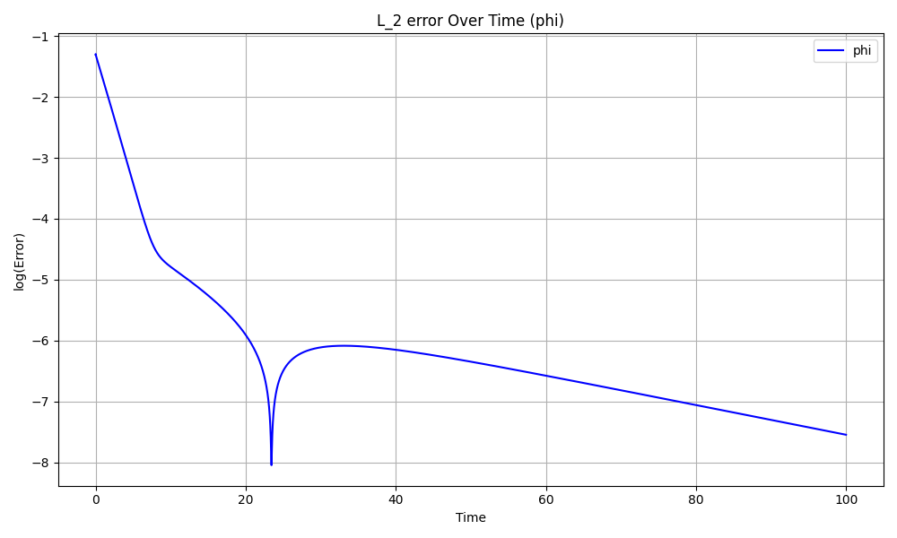
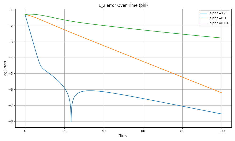
We plot the errors on a logarithmic scale versus time.

Figure 15 shows a clear dependence on $\alpha$. For $\alpha=1$, all primary variables synchronize rapidly: the curves display a steep initial drop and then enter a slower decay regime, consistent with reaching an observation/discretization-limited accuracy. For $\alpha=0.1$, the decay is still robust but noticeably slower; over most of the time interval, the trajectories are close to straight lines on the log scale, indicating approximately exponential decay with a smaller rate. For $\alpha=0.01$, the feedback is too weak on the time horizon $[0,100]$: the errors decrease only mildly and full synchronization is not observed within the final time.

We also report the pressure iterate difference in Figure 15 (top right). Since pressure is only defined up to an additive constant and is obtained here via a pressure-correction update, its curve can remain highly oscillatory even when the primary variables synchronize. Accordingly, the most reliable synchronization indicators are the velocity and phase-field errors.

Figure 15. Log-scale errors for $\alpha_{u}=\alpha_{\phi}=\alpha_{\psi}=\alpha\in\{1,0.1,0.01\}$.. Top left: combined error.Top right: velocity error. Bottom row: componentwise errors in $\phi$ and $\vec{\psi}$.

Test 6: effects of interpolation mesh size

In this test, we examine the dependence of synchronization on the resolution of the observation/interpolation operator $I_{H}$. We keep the physical parameters, time step, and nudging strengths fixed with

$$\alpha_{u}=\alpha_{\phi}=\alpha_{\psi}=1,$$

and vary only the observation mesh size $H$. We consider three observation resolutions (labeled $32\times 32$, $16\times 16$, and $8\times 8$), while maintaining the same overall simulation setup and mismatched initial data as in the preceding tests.

Figure 16 shows a clear monotone trend: finer observations lead to faster and stronger synchronization. The most pronounced sensitivity to $H$ occurs in the velocity component. The velocity error exhibits a steep initial decay and reaches a very small plateau by approximately $t\approx 20$ on the finest observation mesh ($32\times 32$). For $16\times 16$ observations, the same qualitative behavior persists but with a noticeably reduced decay rate. For the coarsest $8\times 8$ observations, the velocity error decreases much more slowly and remains several orders of magnitude larger over the entire interval. This behavior is consistent with the fact that coarser observations cannot constrain finer-scale features of the flow, thereby limiting the achievable synchronization accuracy.

In contrast, the phase-field errors in $\phi$ and $\vec{\psi}$ are less sensitive to $H$ on the time horizon considered, and the combined error is largely governed by the late-time behavior of the auxiliary field $\vec{\psi}$. The energy diagnostics further support this picture: the elastic, mixing, and total energies remain nearly indistinguishable across all observation resolutions, while the kinetic energy exhibits the clearest $H$-dependence, with coarser observations associated with a larger residual kinetic component.

Figure 16. Log-scale errors for three interpolation mesh sizes $H$ (labeled $32\times 32$, $16\times 16$, and $8\times 8$). Top left: combined error. Top right: velocity error. Bottom row: componentwise errors in $\phi$ and $\vec{\psi}$.

Conclusions and Commentary

In this paper we formulated a continuous data assimilation framework for a two-dimensional NSCH-type phase-field model coupled with a transported auxiliary field. The additional transported field contributes an extra stress term in the momentum balance and provides a natural extension of more classical NSCH dynamics arising in complex-fluid and thrombus-inspired phase-field modeling. Our goal was to develop a coarse-observation CDA formulation for this coupled system, identify its basic structural properties, and study its practical behavior through a fully discrete finite element realization.

On the continuous level, we introduced the nudged NSCH–$\psi$ system and recorded two structural properties relevant to the assimilation dynamics. First, we derived a formal energy law for the reference system, showing that the coupled model retains a dissipative structure compatible with the underlying phase-field formulation. Second, we analyzed the behavior of the phase mean and showed that, although the reference phase mass is conserved, the assimilated phase mean is generally influenced by the observation operator and the nudging term. These identities clarify the roles played by the coupled stresses and by the coarse-observation feedback mechanism.

On the discrete level, we proposed a capped fully discrete finite element splitting scheme for the CDA system. The method uses continuous quadratic elements for the phase, chemical potential, velocity, and auxiliary field, together with continuous linear elements for the pressure. The capped phase is used in the evaluation of the phase-dependent coefficients in order to reflect the numerical implementation and preserve admissible coefficient values. Within this framework, we proved one-step well-posedness of the fully discrete problem and established a stepwise a priori estimate for the capped scheme. Although this estimate does not constitute a closed discrete free-energy law and does not provide a full convergence theory, it gives a basic stability bound for the numerical method employed in the experiments.

The numerical experiments illustrate several features of the proposed CDA approach. In particular, they show recovery from strongly mismatched initial data, sensitivity of the synchronization behavior to the nudging strength and the observation resolution, and robustness under boundary forcing. The coarse-indistinguishability experiment further demonstrates that coarse initial information alone may fail to determine the fine-scale evolution uniquely, while the assimilated trajectory is selected by the supplied time-dependent observations. Taken together, these computations indicate that the proposed nudging strategy is effective in practice for this coupled NSCH-type system.

Several directions remain open. One natural next step is to establish a rigorous well-posedness and synchronization theory for the continuous assimilated dynamics under assumptions compatible with the present model. Another is to strengthen the discrete analysis by developing a closed stability theory or a convergence analysis for the capped fully discrete scheme. It would also be of interest to investigate partial-observation scenarios by nudging only the velocity or only the phase field and to characterize the minimal observation content needed for synchronization in this coupled setting. Finally, extending the analysis to three dimensions, or to additional physical couplings motivated by thrombus biomechanics and complex-fluid structure, remains an important and challenging topic.

Declarations

Data Availability Statement

Data sharing is not applicable to this article as no datasets were generated or analysed during the current study.

Funding Statement

This work was partly supported by the Research Fund of Indiana University.

Conflict of Interest Disclosure

All authors certify that they have no affiliations with or involvement in any organization or entity with any competing interests in the subject matter or materials discussed in this manuscript.

Ethics Approval Statement

Not applicable.

Patient Consent Statement

Not applicable.

Permission to Reproduce Material from other Sources

None of the presented material was drawn from other sources.

Clinical Trial Registration

Not applicable.

Authors’ Contribution

The author contributed to all parts of this manuscript.

Acknowledgements

T.S. is greatly thankful to Professor Michael Jolly for the insightful discussions and advice.

References

- [1] (2013) Existence of weak solutions for a diffuse interface model for two-phase flows of incompressible fluids with different densities. J. Math. Fluid Mech. 15, pp. 453–480. External Links: Document Cited by: §1.
- [2] (2013) On an incompressible Navier–Stokes/Cahn–Hilliard system with degenerate mobility. Ann. Inst. H. Poincaré Anal. Non Linéaire 30 (6), pp. 1175–1190. External Links: Document Cited by: §1.
- [3] (2012) Thermodynamically consistent, frame indifferent diffuse interface models for incompressible two-phase flows with different densities. Math. Models Methods Appl. Sci. 22 (3), pp. 1150013. External Links: Document Cited by: §1.
- [4] (2009) On a diffuse interface model for two-phase flows of viscous, incompressible fluids with matched densities. Arch. Rational Mech. Anal. 194 (2), pp. 463–506. External Links: Document Cited by: §1.
- [5] (1998) Diffuse-interface methods in fluid mechanics. Annual Review of Fluid Mechanics 30 (1), pp. 139–165. External Links: Document Cited by: §1.
- [6] (2014) Continuous data assimilation using general interpolant observables. Journal of Nonlinear Science 24 (2), pp. 277–304. External Links: Document Cited by: §1, §2.
- [7] (2017) Three dimensional phase-field investigation of droplet formation in microfluidic flow focusing devices with experimental validation. International Journal of Multiphase Flow 93, pp. 130–141. External Links: Document Cited by: §1.
- [8] (1958) Free energy of a nonuniform system. I. interfacial free energy. The Journal of Chemical Physics 28 (2), pp. 258–267. External Links: Document Cited by: §1.
- [9] (2020) Optimal error estimates for the scalar auxiliary variable finite-element schemes for gradient flows. Numerische Mathematik 145, pp. 167–196. External Links: Document Cited by: Remark 3.2.
- [10] (2020) A novel second-order linear scheme for the Cahn–Hilliard–Navier–Stokes equations. Journal of Computational Physics 423, pp. 109782. Cited by: §1, §3, §3.
- [11] (2024) Convergence analysis of a second order numerical scheme for the Flory–Huggins–Cahn–Hilliard–Navier–Stokes system. Journal of Computational and Applied Mathematics 450, pp. 115981. External Links: Document Cited by: Remark 3.2.
- [12] (2022) Error estimate of a decoupled numerical scheme for the Cahn–Hilliard–Stokes–Darcy system. IMA Journal of Numerical Analysis 42 (3), pp. 2621–2655. External Links: Document Cited by: Remark 3.2.
- [13] (2016) Efficient, adaptive energy stable schemes for the incompressible Cahn–Hilliard–Navier–Stokes phase-field models. Journal of Computational Physics 308, pp. 40–56. Cited by: §1, §3.
- [14] (1968) Numerical solution of the navier–stokes equations. Mathematics of Computation 22 (104), pp. 745–762. Cited by: §3.
- [15] (2022) Continuous data assimilation and long-time accuracy in a interior penalty method for the Cahn–Hilliard equation. Appl. Math. Comput. 424, pp. 127042. External Links: Document Cited by: §1.
- [16] (2017) Convergence analysis and error estimates for a second order accurate finite element method for the Cahn–Hilliard–Navier–Stokes system. Numerische Mathematik 137, pp. 495–534. External Links: Document Cited by: Remark 3.2.
- [17] (2016) Abridged continuous data assimilation for the 2D Navier–Stokes equations utilizing measurements of only one component of the velocity field. J. Math. Fluid Mech. 18, pp. 1–23. External Links: Document Cited by: §1.
- [18] (2017) Continuous data assimilation for a 2D Bénard convection system through horizontal velocity measurements alone. Journal of Nonlinear Science 27, pp. 1065–1087. External Links: Document Cited by: §1.
- [19] (2007) Analysis of finite element approximations of a phase field model for two-phase fluids. Mathematics of Computation 76 (258), pp. 539–571. External Links: Document Cited by: Remark 3.2.
- [20] (2006) Fully discrete finite element approximations of the Navier–Stokes–Cahn–Hilliard diffuse interface model for two-phase fluid flows. SIAM Journal on Numerical Analysis 44 (3), pp. 1049–1072. External Links: Document Cited by: Remark 3.2.
- [21] (2016) A discrete data assimilation scheme for the solutions of the two-dimensional Navier–Stokes equations and their statistics. SIAM J. Appl. Dyn. Syst. 15 (4), pp. 2109–2142. External Links: Document Cited by: §1.
- [22] (2010) Asymptotic behavior of a Cahn–Hilliard–Navier–Stokes system in 2D. Ann. Inst. H. Poincaré Anal. Non Linéaire 27 (1), pp. 401–436. External Links: Document Cited by: §1.
- [23] (2014) An efficient scheme for a phase field model for the moving contact line problem with variable density and viscosity. Journal of Computational Physics 272, pp. 704–718. Cited by: §3.
- [24] (2016) A computational study of a data assimilation algorithm for the two-dimensional Navier–Stokes equations. Communications in Computational Physics 19 (4), pp. 1094–1110. External Links: Document Cited by: §1.
- [25] (2023) Existence and regularity of strong solutions to a nonhomogeneous Kelvin–Voigt–Cahn–Hilliard system. Journal of Differential Equations 372, pp. 612–656. External Links: Document Cited by: §1, §1.
- [26] (2019) Uniqueness and regularity for the Navier–Stokes–Cahn–Hilliard system. SIAM Journal on Mathematical Analysis 51 (3), pp. 2535–2574. External Links: Document Cited by: §1.
- [27] (2022) Attractors for the Navier–Stokes–Cahn–Hilliard system. Discrete and Continuous Dynamical Systems – Series S 15 (8), pp. 2249–2274. External Links: Document Cited by: §1.
- [28] (1986) Finite element methods for navier–stokes equations: theory and algorithms. Springer. Cited by: §3.
- [29] (2023) A phase-field system arising from multiscale modeling of thrombus biomechanics in blood vessels: local well-posedness in dimension two. Discrete and Continuous Dynamical Systems – Series S 16 (9), pp. 2364–2425. External Links: Document Cited by: §1, §1.
- [30] (2015) A second order in time, uniquely solvable, unconditionally stable numerical scheme for Cahn–Hilliard–Navier–Stokes equation. Journal of Computational Physics 290, pp. 139–156. Cited by: §1, §3, §3.
- [31] (2021) Global well-posedness of a Navier–Stokes–Cahn–Hilliard system with chemotaxis and singular potential in 2D. Journal of Differential Equations 297, pp. 47–80. External Links: Document Cited by: §1.
- [32] (1993) Upper bounds on the number of determining modes, nodes, and volume elements for the Navier–Stokes equations. Indiana University Mathematics Journal 42 (3), pp. 875–887. External Links: Document Cited by: §1.
- [33] (2022-04) Local well-posedness of a three-dimensional phase-field model for thrombus and blood flow. Note: arXiv:2204.07527v1 External Links: 2204.07527 Cited by: §1, §1, §2.
- [34] (2020) Approximate continuous data assimilation of the 2D Navier–Stokes equations via the Voigt-regularization with observable data. Evol. Equ. Control Theory 9 (3), pp. 733–751. External Links: Document Cited by: §1.
- [35] (2005) On hydrodynamics of viscoelastic fluids. Communications on Pure and Applied Mathematics 58 (11), pp. 1437–1471. External Links: Document Cited by: §1, §1.
- [36] (2017) Error analysis of a mixed finite element method for a Cahn–Hilliard–Hele–Shaw system. Numerische Mathematik 135, pp. 679–709. External Links: Document Cited by: Remark 3.2.
- [37] (2017) The Cahn–Hilliard equation and some of its variants. AIMS Mathematics 2 (3), pp. 479–544. External Links: Document Cited by: §1.
- [38] (2019) The Cahn-Hilliard equation. CBMS-NSF Regional Conference Series in Applied Mathematics, Vol. 95, Society for Industrial and Applied Mathematics (SIAM), Philadelphia, PA. Note: Recent advances and applications Cited by: §1.
- [39] (2018) The scalar auxiliary variable (SAV) approach for gradient flows. Journal of Computational Physics 353, pp. 407–416. Cited by: §3.
- [40] (2015) Decoupled, energy stable schemes for phase-field models of two-phase incompressible flows. SIAM Journal on Numerical Analysis 53 (1), pp. 279–296. Cited by: §1, §3.
- [41] (2024) An unconditional energy stable data assimilation scheme for Navier–Stokes–Cahn–Hilliard equations with local discretized observed data. Computers & Mathematics with Applications 164, pp. 21–33. External Links: Document Cited by: §1, §3.
- [42] (1969) Sur l’approximation de la solution des équations de Navier–Stokes par la méthode des pas fractionnaires (i). Archive for Rational Mechanics and Analysis 32, pp. 135–153. Cited by: §3.
- [43] (1977) Navier–stokes equations: theory and numerical analysis. North-Holland. Cited by: §3.
- [44] (2025) On the inadequacy of nudging data assimilation algorithms for non-dissipative systems. Discrete and Continuous Dynamical Systems – Series S. Note: Published online Oct. 22, 2025 External Links: Document Cited by: §1.
- [45] (2017) Well-posedness of a diffuse-interface model for two-phase incompressible flows with thermo-induced Marangoni effect. European Journal of Applied Mathematics 28 (3), pp. 380–434. External Links: Document Cited by: §1.
- [46] (2019) Three-phase model of visco-elastic incompressible fluid flow and its computational implementation. Communications in Computational Physics 25 (2), pp. 586–624. External Links: Document Cited by: §1.
- [47] (2017) Model predictions of deformation, embolization and permeability of partially obstructive blood clots under variable shear flow. Journal of The Royal Society Interface 14 (136), pp. 20170441. External Links: Document Cited by: §1.
- [48] (2022) Continuous data assimilation algorithm for the two dimensional Cahn–Hilliard–Navier–Stokes system. Applied Mathematics & Optimization 85. External Links: Document Cited by: §1.
- [49] (2021) Second-order decoupled energy-stable schemes for Cahn–Hilliard–Navier–Stokes equations. Journal of Computational Physics 443, pp. 110536. Cited by: §1, §3.
- [50] (2020) A three-dimensional phase-field model for multiscale modeling of thrombus biomechanics in blood vessels. PLOS Computational Biology 16 (4), pp. e1007709. External Links: Document Cited by: §1, §1.