Manifold-Adapted Sparse RBF-SINDy:
Unbiased Library Construction and Unsupervised Discovery of
Dynamical States in Turbulent Wall Flows

Abstract

The turbulent attractor in wall-bounded flow is not a structureless strange set: it has a skeleton of dynamically distinct states, connected by rare but directed transitions, whose geometry is imprinted on the invariant measure of the phase-space trajectory. We show that this skeleton is recoverable from wall measurements alone — wall pressure and wall-shear stress — without physical labels or prior knowledge, provided the data-driven function library used to learn the dynamics is constructed to respect the intrinsic geometry of the attractor rather than the extrinsic variance hierarchy of the POD representation. Standard sparse-identification approaches introduce two structural biases at the library construction stage. The steep energy decay of POD spectra causes the Euclidean distance in $k$-means to be dominated by the leading modes, collapsing all basis-function centres into a low-dimensional subspace and leaving the transition dynamics without library coverage. Separately, turbulent trajectories slow near quasi-invariant flow states, so uniform time-stepping over-represents those states relative to the physical invariant measure and under-samples the fast transitional passages between them. Both biases are corrected by resampling the trajectory uniformly in arc-length before clustering, and by replacing the Euclidean metric in $k$-means with the Mahalanobis metric derived from the local covariance of each cluster. The arc-length resampling drives the empirical measure towards the physical invariant measure; the Mahalanobis metric produces ellipsoidal basis functions whose support is adapted to the local Riemannian geometry of the attractor at each cluster, rather than to the global variance hierarchy of the POD spectrum. A single global sparse regression on this corrected library, with centre allocation weighted by dynamical coherence and cluster population, completes the model. Applied to a minimal turbulent channel at $Re_{\tau}=180$, the corrected latent-space geometry renders the two phases of the near-wall autonomous cycle directly visible to unsupervised clustering: stable streak attractors and burst-initiating instabilities separate into two sharp populations without any physical input, mapping onto the exact coherent structure skeleton of the flow. This organisation is absent when standard biased approaches are used. The learned model recovers the correct invariant measure, saturates the Lyapunov predictability horizon set by the intrinsic chaos of the flow, and furnishes a differentiable vector field on which invariant solutions can be located directly by Newton iteration.

1 Introduction

The dynamics of near-wall turbulence are organised around a self-sustaining cycle of elongated low-speed streaks, their sinuous instability, and a subsequent breakdown and regeneration (Jiménez and Pinelli, 1999). This cycle operates on timescales of order $100t^{+}$ and is accessible, at least in part, through measurements at the wall: the pressure and shear-stress footprint of the near-wall structures is coherent enough that reduced-order models driven exclusively by wall quantities can capture a significant fraction of the flow dynamics (Jiménez and Moin, 1991).

Sparse identification of nonlinear dynamics (SINDy) (Brunton et al., 2016), combined with a POD encoding of the wall-measurement snapshots, offers a natural framework for this problem. One seeks a sparse ordinary differential equation $\dot{\bm{a}}=\bm{\Theta}(\bm{a})\bm{\xi}$ in the space of POD latent coefficients, assembled from a library of candidate functions $\bm{\Theta}$. For turbulent flows, global polynomial libraries are insufficiently flexible, and radial basis functions (RBFs) placed on the attractor (Reinbold et al., 2020; Loiseau and Brunton, 2018) provide a better approximation basis. The idea of partitioning the phase-space trajectory by $k$-means clustering and building a reduced model on that partition was introduced by Kaiser et al. (2014) as cluster-based reduced-order modelling (CROM), and extended to continuous-time network dynamics by Fernex et al. (2021). Those approaches model inter-cluster dynamics by a discrete Markov transition matrix; the present work replaces that discrete jump model with a continuous, differentiable sparse ODE whose library is built from the same cluster geometry, enabling trajectory integration and, as discussed below, direct access to invariant solutions of the learned system. A related but architecturally distinct line of work replaces the Markov model with a collection of local intrusive ROMs, one per cluster, switching between them via a nearest-centroid affiliation function. Colanera and Magri (2025) demonstrate this quantized local ROM (ql-ROM) strategy on the Kuramoto–Sivashinsky and Kolmogorov flow equations, showing gains in numerical stability and long-time statistical accuracy over a single global Galerkin model. Because ql-ROMs require the governing equations for each local Galerkin projection and introduce coordinate discontinuities at cluster boundaries — which the authors identify as a limitation requiring future treatment — they are not directly applicable to observation-limited settings such as the wall-measurement problem considered here. The present framework is non-intrusive throughout and produces a globally smooth vector field, so no switching discontinuities arise and the full benefits of a differentiable ODE are retained.

The difficulty is that the POD latent space of a turbulent flow is neither flat nor isotropic. POD spectra decay rapidly: the variance in the leading mode can exceed that in the last retained mode by three or four orders of magnitude. A $k$-means algorithm that uses the Euclidean distance on this space will distribute its centres to minimise inertia in the high-variance directions, leaving the low-variance modes — which carry the inter-state transition structure that governs the long-time dynamics — without any RBF support. A separate but equally damaging effect comes from the non-uniform speed of turbulent trajectories. Near quasi-invariant states such as the laminar streak phase, trajectories slow substantially; uniform time-stepping therefore over-represents those states relative to the physical invariant measure and under-samples the fast bursting transitions. When $k$-means is applied to uniformly sampled data, the cluster geometry inherits this distortion, placing additional centres in the already over-represented slow regions.

The consequences are not merely a degradation in regression accuracy. Because both biases misrepresent the attractor geometry, the learned model converges to the wrong invariant measure: it may reproduce short-time trajectories reasonably well but fails to recover the correct long-time energy statistics and the dynamical state structure of the flow. The goal of the present work is to correct both biases at the level of library construction, before any regression is performed, so that the resulting model is consistent with the physical invariant measure from the outset.

The correction proceeds in two steps. The trajectory is first resampled uniformly in arc-length, which redistributes the sampling density in proportion to the local phase-space speed and thereby approximates uniform sampling with respect to the invariant measure. The $k$-means clustering is then performed with the Mahalanobis distance derived from the local covariance of each cluster rather than the Euclidean distance. This stretches the effective distance along low-variance directions so that cluster boundaries, and the RBF centres derived from them, are distributed uniformly across the full latent-space geometry rather than compressed into the subspace of the leading modes. The resulting library feeds a single global sparse regression, with no local models and no model switching.

When this corrected framework is applied to a minimal turbulent channel at $Re_{\tau}=180$, the clustering step reveals something not visible with standard approaches: the trajectory organises into two sharply separated populations in the space of cluster residence time and phase-space velocity coherence, reproducing the streak and burst phases of the near-wall cycle without any physical input. These two populations are interpretable as the data-driven counterpart of the exact coherent structure (ECS) skeleton that organises the turbulent attractor (Nagata, 1990; Cvitanović and Gibson, 2010; Kawahara et al., 2012): the high-residence cluster neighbourhood approximates the lower-branch laminar-streak ECS, while the low-residence neighbourhood approximates the upper-branch saddle-type structures that initiate the burst.

2 Problem formulation

2.1 POD encoding

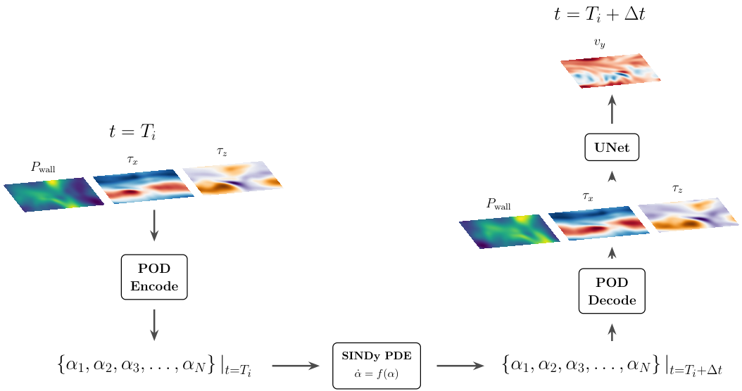
The overall modelling pipeline is sketched in figure 1. Let $\bm{u}(\bm{x},t)\in\mathbb{R}^{N}$ denote the discretised wall-measurement field, consisting of $P_{\mathrm{wall}}$, $\tau_{x}$, and $\tau_{z}$ sampled on both walls. Given $M$ snapshots $\{\bm{u}_{i}\}_{i=1}^{M}$, the fluctuation matrix $\bm{U}^{\prime}=\bm{U}-\bar{\bm{u}}\bm{1}_{M}^{\top}$ is formed and a truncated randomised SVD $\bm{U}^{\prime}\approx\bm{\Phi}_{r}\bm{\Sigma}_{r}\bm{V}_{r}^{\top}$ is computed, retaining $r$ modes that account for a fraction $\eta\geq 0.99$ of the total variance (Sirovich, 1987). The latent state $\bm{a}(t)=\bm{\Phi}_{r}^{\top}\bm{u}^{\prime}(\cdot,t)\in\mathbb{R}^{r}$ encodes the snapshot, and $\bm{u}^{\prime}\approx\bm{\Phi}_{r}\bm{a}$ decodes it. Time derivatives $\dot{\bm{a}}$ are estimated by second-order centred finite differences.

Figure 1: Schematic of the modelling pipeline. Wall measurements $\{P_{\mathrm{wall}},\tau_{x},\tau_{z}\}$ at time $T_{i}$ are encoded onto POD latent coefficients $\{\alpha_{j}\}$, advanced by the learned RBF-SINDy ODE, and decoded back to wall fields at time $T_{i}+\Delta t$.

2.2 Sparse identification in the latent space

The dynamics of the latent state are approximated by

$$\dot{\bm{a}}=\sum_{k=1}^{K}\xi_{k}\,\phi_{k}(\bm{a}),$$ (1)

where $\{\phi_{k}\}_{k=1}^{K}$ are the $K$ library functions and $\bm{\xi}\in\mathbb{R}^{K\times r}$ is a sparse matrix of amplitude coefficients. The library functions are fixed entirely by the data geometry, as described in section 3; SINDy operates only on the amplitudes, solving the linear regression $\dot{A}\approx\bm{\Theta}(A)\bm{\xi}$ and enforcing sparsity by either sequentially thresholded least squares (STLS), or penalising the regression with an $L_{1}$ term (Brunton et al., 2016). The library $\bm{\Theta}$ consists of $K$ radial basis functions (RBFs) centred at points $\{\bm{c}_{k}\}_{k=1}^{K}$ in the latent space, augmented with the $r$ linear terms $\{a_{j}\}_{j=1}^{r}$.

Radial basis functions of the form $\phi_{k}(\bm{a})=\varphi(\|\bm{a}-\bm{c}_{k}\|)$ are a classical tool for approximating smooth functions on $\mathbb{R}^{r}$ (Buhmann, 2003; Wendland, 2004). For any choice of strictly positive definite kernel $\varphi$, the set $\{\phi_{k}\}_{k=1}^{K}$ spans a reproducing kernel Hilbert space (RKHS) and can approximate any continuous function on a compact domain to arbitrary accuracy as $K\to\infty$ with centres dense in the domain (Micchelli, 1986). In practice $K$ is finite and the centres are placed on or near the attractor, so the library is adapted to the support of the invariant measure rather than to a uniform grid. The linear terms are retained to capture any residual affine structure and to improve conditioning of the regression problem.

Among admissible kernels, the Gaussian RBF

$$\varphi(d)=\exp\!\left(-\frac{d^{2}}{2\sigma^{2}}\right)$$

is a natural choice in a dynamical-systems context. Here $d=\|\bm{a}-\bm{c}_{k}\|$ denotes the Euclidean distance between the state $\bm{a}$ and the centre $\bm{c}_{k}$ of the $k$-th kernel, and $\sigma$ is the bandwidth controlling the spatial extent of the basis function. This expression corresponds to the isotropic form of the Gaussian kernel, in which the same width $\sigma$ is used in all directions of the $r$-dimensional state space.

The Gaussian RBF possesses several desirable properties: i) it is infinitely differentiable, ensuring that the learned right-hand side $f(\bm{a})=\bm{\Theta}(\bm{a})\bm{\xi}$ is smooth and well posed for numerical integration; ii) its Fourier transform is also Gaussian, providing spectral locality: each RBF term contributes primarily within a well-defined neighbourhood of its centre, without introducing spurious long-range interactions between distant centres; iii) it aligns naturally with the local geometry of the data distribution. The advantages of this feature will become particularly evident once the Mahalanobis metric is introduced in Section 3.

Each Gaussian RBF is characterised by two sets of parameters: its centre $\bm{c}_{k}\in\mathbb{R}^{r}$ and its width (or bandwidth) $\sigma_{k}\in\mathbb{R}^{+}$. The centre determines where the basis function acts in state space, while the width controls the spatial extent of its influence.

In the simplest isotropic case a single scalar width $\sigma\in\mathbb{R}^{+}$ is shared across all $r$ directions. Each RBF then requires $r+1$ parameters: the $r$ coordinates of the centre and one bandwidth. In the anisotropic case the scalar width is replaced by a full $r\times r$ symmetric positive-definite matrix $\bm{\Sigma}$, allowing different spreads and orientations in state space; this introduces $r+r(r+1)/2$ parameters per function.

In the present framework the centres $\bm{c}_{k}$ are determined by arc-length discretisation of the latent trajectory, with spacing weighted by the local phase-space speed $\|\dot{\bm{a}}\|$, so that dynamically active regions receive a denser coverage of centres. The width matrices are obtained from the per-cluster sample covariance matrices $\bm{\Sigma}_{k}$, computed from the snapshots assigned to each cluster and inverted to yield the precision matrices $\bm{\Sigma}_{k}^{-1}$ that define the anisotropic kernel shape.

Because both centres and widths are fixed directly from the data geometry before the regression step, the identification problem in (1) remains purely linear in the amplitude coefficients $\bm{\xi}$. This provides a significant computational and algorithmic advantage over approaches that optimise kernel centres, widths, and coefficients jointly, where the resulting problem is nonlinear and considerably harder to condition.

The procedure used to construct these centres and precision matrices is described in the next section.

3 Methodology

3.1 Coordinate bias from Euclidean clustering

The POD singular values satisfy $\sigma_{1}\geq\sigma_{2}\geq\cdots\geq\sigma_{r}$ and $\mathrm{Var}(a_{j})\propto\sigma_{j}^{2}$. In turbulent channel flow the ratio $\sigma_{1}^{2}/\sigma_{r}^{2}$ typically exceeds $10^{3}$. The standard $k$-means algorithm minimises the total Euclidean inertia

$$\mathcal{I}=\sum_{k=1}^{K}\sum_{i\in\mathcal{C}_{k}}\left\|\bm{a}(t_{i})-\bm{c}_{k}\right\|^{2}=\sum_{j=1}^{r}\sum_{k,i}(a_{j}(t_{i})-c_{k,j})^{2},$$ (2)

and since each term in the $j$-sum scales with $\sigma_{j}^{2}$, the optimiser invests all $K$ centres to resolve the first two or three directions. The RBFs placed there have negligible support in the remaining directions, which carry the transition dynamics between flow states and determine the invariant measure.

3.2 Temporal sampling bias

The empirical measure from uniform time-stepping, $\mu_{\Delta}=M^{-1}\sum_{i}\delta_{\bm{a}(t_{i})}$, is related to the physical invariant measure $\mu_{\infty}$ by

$$\frac{d\mu_{\Delta}}{d\mu_{\infty}}(\bm{a})\propto\left\|\dot{\bm{a}}(\bm{a})\right\|^{-1}.$$ (3)

Regions where the trajectory is slow accumulate many snapshots; fast transitional regions are sparsely sampled. When $k$-means is applied to $\mu_{\Delta}$, centres are pulled towards the over-represented slow regions and the regression targets are dominated by them, systematically misrepresenting the dynamics that govern transitions between attractors.

The two biases are independent and must each be corrected separately. Coordinate-correcting methods such as ISOMAP change the extrinsic representation of the manifold but leave the temporal sampling distribution unchanged; arc-length resampling corrects the measure but not the metric. Only their combination yields a library that is simultaneously unbiased in geometry and in sampling density.

3.3 Arc-length resampling

The trajectory $\{\bm{a}(t_{i})\}_{i=1}^{M}$ is resampled at $M$ equally spaced points along its arc-length

$$\ell_{i}=\sum_{j=1}^{i-1}\left\|\bm{a}(t_{j+1})-\bm{a}(t_{j})\right\|,\quad i=1,\ldots,M,$$ (4)

by interpolating at the uniform grid $\ell^{*}_{n}=n\,\ell_{M}/(M-1)$. The resampled empirical measure $\hat{\mu}$ approximates the arc-length measure $d\ell/\ell_{M}$ and satisfies

$$\frac{d\hat{\mu}}{d\mu_{\Delta}}(\bm{a})\propto\left\|\dot{\bm{a}}(\bm{a})\right\|^{2},$$ (5)

up-weighting fast segments relative to slow ones. For ergodic systems with bounded phase-space speed, $\hat{\mu}\to\mu_{\infty}$ as $M\to\infty$, and all subsequent steps operate on the resampled trajectory $\{\hat{\bm{a}}_{n}\}$.

3.4 Arc-length discretisation and cluster assignment

The arc-length resampled trajectory $\{\hat{\bm{a}}_{n}\}$ defines a one-dimensional curve in $\mathbb{R}^{r}$. This curve is discretised into $K$ segments by placing $K$ centre points $\{\bm{c}_{k}\}_{k=1}^{K}$ at equally spaced arc-length positions along it, with the spacing $\Delta s$ stretched locally in proportion to the phase-space speed $\|\dot{\bm{a}}\|$ so that dynamically active regions receive denser coverage. Each resampled snapshot $\hat{\bm{a}}_{n}$ is then assigned to the nearest centre in the Euclidean sense, defining $K$ disjoint clusters $\mathcal{C}_{k}=\{n:k=\arg\min_{j}\|\hat{\bm{a}}_{n}-\bm{c}_{j}\|\}$.

For each cluster $k$ the sample covariance is computed from the assigned snapshots,

$$\bm{\Sigma}_{k}=\frac{1}{|\mathcal{C}_{k}|}\sum_{n\in\mathcal{C}_{k}}(\hat{\bm{a}}_{n}-\bm{c}_{k})(\hat{\bm{a}}_{n}-\bm{c}_{k})^{\top}+\varepsilon I_{r},$$ (6)

where the regularisation $\varepsilon I_{r}$ prevents singularity in under-populated clusters. The precision matrix $\bm{\Sigma}_{k}^{-1}$ is obtained by direct inversion and encodes the local geometry of the attractor at each centre: it stretches distances along low-variance directions so that the support of the corresponding RBF reflects the actual shape of the data cloud rather than the global POD variance hierarchy. The cluster count $K$ is determined automatically by G-means (Hamerly and Elkan, 2003), which tests each candidate cluster for Gaussianity and subdivides it if the test fails.

Figure 2 illustrates the difference between isotropic and Mahalanobis RBFs for representative clusters: the isotropic RBF ignores the anisotropy of the cluster, while the Mahalanobis RBF aligns its support with the local data distribution.

Figure 2: Comparison of isotropic Gaussian RBF (left) and Mahalanobis Gaussian RBF (right) for the same cluster centroid. The isotropic function assigns equal bandwidth in all directions regardless of the local data geometry; the Mahalanobis function stretches along low-variance directions and compresses along high-variance ones, matching the ellipsoidal shape of the cluster.

The $k$-th library function is the Mahalanobis Gaussian RBF:

$$\phi_{k}(\bm{a})=\exp\!\left(-(\bm{a}-\bm{c}_{k})^{\top}\bm{\Sigma}_{k}^{-1}(\bm{a}-\bm{c}_{k})\right).$$ (7)

The level sets of $\phi_{k}$ are ellipsoids whose axes are aligned with the eigenvectors of $\bm{\Sigma}_{k}$ and scaled by the corresponding eigenvalues, so the support of each basis function is geometrically congruent with the local data distribution it represents. Figure 3 shows the one-sigma Mahalanobis surfaces for three representative clusters, illustrating the strongly anisotropic and heterogeneous geometry of the attractor that isotropic RBFs would fail to capture.

3.5 Coherence-weighted centre allocation

The allocation of the centre budget $K$ across clusters follows

$$K_{k}\propto(1-c_{k})\sqrt{N_{k}},$$ (8)

where $N_{k}=|\mathcal{C}_{k}|$ and

$$c_{k}=\frac{1}{|\mathcal{C}_{k}|}\sum_{i\in\mathcal{C}_{k}}\frac{\dot{\bm{a}}(t_{i})\cdot\dot{\bm{a}}(t_{i+1})}{\left\|\dot{\bm{a}}(t_{i})\right\|\left\|\dot{\bm{a}}(t_{i+1})\right\|}$$ (9)

is the mean cosine similarity of consecutive phase-space velocity vectors within cluster $k$. Clusters with low coherence (rapidly changing trajectory direction) receive more centres; larger clusters receive proportionally more coverage. Within each cluster the centres are distributed by farthest-point sampling in the Mahalanobis metric.

Figure 3: Three representative clusters (1, 10, 20) visualised in the space of the first three standardised POD coefficients. The ellipsoids represent the one-sigma Mahalanobis surface $(\bm{a}-\bm{c}_{k})^{\top}\bm{\Sigma}_{k}^{-1}(\bm{a}-\bm{c}_{k})=1$. The varying size and orientation reflect the strongly anisotropic and heterogeneous geometry of the attractor.

3.6 Algorithm recap

Offline training proceeds as follows. A randomised SVD of the fluctuation snapshot matrix yields $\bm{\Phi}_{r}$ and the latent trajectory $A$. Time derivatives $\dot{A}$ are estimated by centred differences. The trajectory is resampled uniformly in arc-length to obtain $\hat{A}$, which is then discretised into $K$ clusters (with $K$ from G-means) by arc-length centre placement and nearest-neighbour assignment. For each cluster the sample covariance $\bm{\Sigma}_{k}$ is computed and inverted to give the precision matrix $\bm{\Sigma}_{k}^{-1}$, fully defining the RBF library $\bm{\Theta}$ via (7). Centre allocation follows (8). With the library fixed, STLS (Brunton et al., 2016) solves the linear regression $\dot{A}\approx\bm{\Theta}(A)\bm{\xi}$ for the sparse amplitude matrix $\bm{\xi}$.

Online prediction from an initial wall-measurement snapshot $\bm{u}_{0}$ requires the encoding $\bm{a}_{0}=\bm{\Phi}_{r}^{\top}(\bm{u}_{0}-\bar{\bm{u}})$, followed by RK4 integration of $\dot{\bm{a}}=\bm{\Theta}(\bm{a})\bm{\xi}$, and decoding $\bm{u}=\bm{\Phi}_{r}\bm{a}+\bar{\bm{u}}$. The cost per time step is $O(sr)$ for $s$ active RBF terms, compared to $O(N\log N)$ for spectral DNS, giving online speedups of $10^{3}$–$10^{5}$.

4 Results

4.1 Dataset and POD encoding

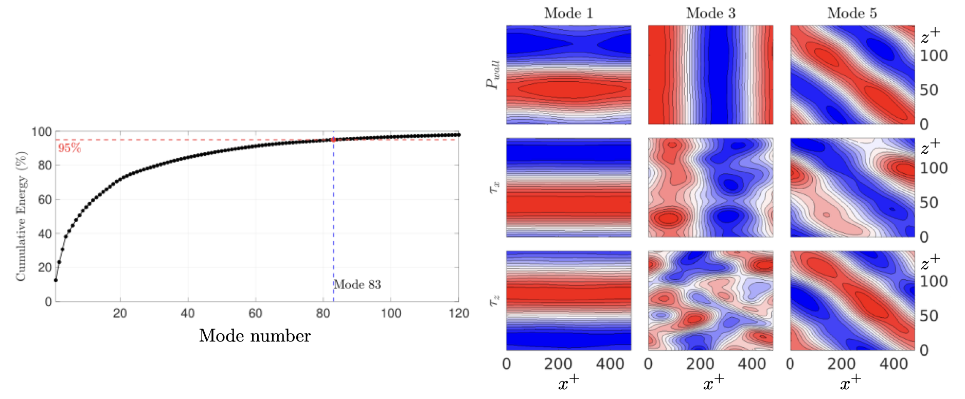
The training data consist of $M=20{,}000$ snapshots of $\{P_{\mathrm{wall}},\,\tau_{x},\,\tau_{z}\}$ from a minimal turbulent channel at $Re_{\tau}=180$ (Jiménez and Moin, 1991), sampled at intervals of $0.5t^{+}$. A randomised SVD retains $r=83$ modes accounting for 95% of the total wall-measurement variance, as shown in figure 4. Mode 1 reflects the large-scale pressure signature of elongated streaks; Modes 3 and 5 capture the streamwise-periodic and oblique patterns associated with streak instability.

Figure 4: Left: cumulative energy as a function of POD mode index, with the 95% threshold at mode 83 indicated. Right: wall-pressure $P_{\mathrm{wall}}$, streamwise shear $\tau_{x}$, and spanwise shear $\tau_{z}$ contours for modes 1, 3 and 5 (columns), illustrating the physical content of the leading modes.

4.2 Dynamical states recovered by unsupervised clustering

G-means clustering of the corrected latent trajectory returns $K=32$ clusters. For each cluster we compute the mean residence time and velocity coherence (9); the result is shown in figure 5.

Figure 5: Average residence time versus velocity coherence for the 32 clusters returned by G-means on the arc-length resampled, Mahalanobis-corrected trajectory. Two populations are clearly separated: high-residence / low-coherence clusters (upper left) correspond to quasi-steady streak states; low-residence / high-coherence clusters (lower right) correspond to burst-initiating instabilities.

The distribution is sharply bimodal. The first population, exemplified by clusters 7, 8 and 21 (figure 6), has high residence time and low velocity coherence. The trajectory settles here for extended periods, with the phase-space velocity changing direction erratically rather than following a coherent path. The wall fields reconstructed from the cluster centroids show large-scale, nearly spanwise-uniform pressure distributions and strongly streamwise-aligned wall-shear stress — the signature of the quasi-steady elongated streak state that constitutes the laminar phase of the near-wall cycle (Jiménez and Pinelli, 1999).

Figure 6: Three representative high-residence / low-coherence clusters (7, 8, 21). Left: their positions in the (coherence, residence time) plane. Right: reconstructed wall fields $P_{\mathrm{wall}}$, $\tau_{x}$, $\tau_{z}$ at each cluster centroid, showing the large-scale, spanwise-uniform streak signature.

The second population, exemplified by clusters 3, 10 and 16 (figure 7), has short residence time and high velocity coherence. The trajectory passes through these states rapidly, with the phase-space velocity strongly aligned from one snapshot to the next. The wall fields are oblique and strongly three-dimensional, consistent with the sinuous instability of streaks and the initiation of a turbulent burst.

Figure 7: Three representative low-residence / high-coherence clusters (3, 10, 16). Left: their positions in the (coherence, residence time) plane. Right: reconstructed wall fields at each cluster centroid, showing the oblique, three-dimensional instability signature.

This bimodal organisation maps directly onto the streak and burst phases identified by Jiménez and Pinelli (1999) through a completely independent analysis. It emerges here with no physical assumptions, as a geometric consequence of the corrected latent-space discretisation. When the same clustering is applied to uniformly sampled data with the Euclidean metric, the bimodal structure is absent: coordinate bias compresses the centre distribution into the subspace of the leading modes and temporal sampling bias inflates the apparent extent of the slow streak states, obscuring the separation between the two populations.

Figure 8: Cluster-to-cluster transition probability matrix $P_{kj}$, computed from the arc-length resampled trajectory. The block structure reflects the separation between stable streak clusters and unstable burst-initiating clusters, with directed transitions between the two populations.

The two populations also admit a precise dynamical interpretation within the exact coherent structure (ECS) framework for turbulent shear flows (Kawahara et al., 2012). That framework identifies the turbulent attractor with a skeleton of invariant solutions — equilibria, travelling waves, and unstable periodic orbits — connected by heteroclinic and homoclinic orbits, with the statistical properties of turbulence recoverable as weighted averages over these solutions. The high-residence / low-coherence clusters recovered here correspond to the neighbourhoods of lower-branch ECS: laminar-like, low-dissipation states near which the trajectory lingers for extended periods, analogous to the streak-dominated lower-branch equilibrium of the near-wall cycle (Jiménez and Pinelli, 1999). The low-residence / high-coherence clusters correspond to saddle-type or upper-branch ECS through which the trajectory passes rapidly and directedly on its way to triggering a burst and returning to the streak attractor. The precision matrices $\bm{\Sigma}_{k}^{-1}$ of the Mahalanobis clusters are natural geometric descriptors of these neighbourhoods: the ellipsoidal one-sigma surface of a high-residence cluster is elongated along the directions of slow approach to and departure from the nearby invariant solution, directly encoding the local stable and unstable manifold structure. The cluster-to-cluster transition matrix (figure 8) then provides the probabilistic coarse-graining of the heteroclinic connections between these ECS families, constituting a directed Markov skeleton of the near-wall cycle entirely consistent with what the ECS framework predicts on theoretical grounds. That this structure emerges from wall-observable data alone, without access to the interior velocity field, reflects the wall-attached character of the relevant ECS at $Re_{\tau}=180$: the pressure and shear-stress footprint of the near-wall structures is coherent enough to make their phase-space neighbourhoods distinguishable in the POD latent space of the wall measurements.

The cluster-to-cluster transition probability matrix $P_{kj}$ (figure 8) exhibits a clear block structure, with rare but directed transitions from streak-state clusters to burst-initiating clusters and rapid return. This directed Markov skeleton of the autonomous cycle is a natural output of the corrected clustering. The coherence-weighted allocation concentrates centres in the burst-initiating clusters, which have low coherence and high dynamical complexity, consistently with the weighting prescribed by equation (8).

Figure 9: Time derivatives of latent coefficients $\dot{\alpha}_{j}$ for modes $j=1,3,5,7$ (rows): ROM integration (blue) versus DNS finite differences (orange) over $t^{+}\in[0,600]$. The ROM reproduces the dominant oscillations and burst excursions across all retained modes without low-frequency drift or amplitude inflation.

4.3 Mode time-traces: ROM versus DNS

The most direct test of the learned ODE is a comparison of the temporal evolution of individual latent coefficients $\alpha_{j}(t)$ against the DNS reference over a contiguous integration window. Figure 9 shows the time derivatives $\dot{\alpha}_{j}$ produced by the ROM alongside the finite-difference values from the DNS for modes $j=1,3,5,7$ over $t^{+}\in[0,600]$, corresponding to approximately six near-wall cycle periods. The agreement is close across all four modes throughout the window, with the ROM capturing the amplitude and phase of the dominant oscillations as well as the sharper excursions associated with burst events visible as isolated large-amplitude dips in $\dot{\alpha}_{1}$ near $t^{+}\approx 50$ and $t^{+}\approx 320$. The higher modes $\dot{\alpha}_{5}$ and $\dot{\alpha}_{7}$ show somewhat larger pointwise errors at burst events, consistent with the expectation that energy cascades to higher POD modes during the burst phase and the Lyapunov divergence is fastest there. Crucially, the ROM does not exhibit the low-frequency drift or amplitude inflation that characterises poorly conditioned RBF regressions, confirming that the Mahalanobis library construction and the STLS sparsification together produce a well-conditioned model.

Figure 10: Lyapunov spectrum of the learned ROM, ordered by exponent index. Positive exponents (red) define the chaotic core; negative exponents (blue) define the stable complement. Error bars indicate variability across trajectory segments. The leading exponent $\lambda_{1}\approx 0.2\,\mathrm{s}^{-1}$ sets the predictability horizon $t^{*}\approx 5t^{+}$.

4.4 Dynamical fidelity of the learned model

The central question for any data-driven ROM is whether it has learned the correct dynamics or merely fitted the training trajectory. Three complementary diagnostics address this.

The first is invariant measure recovery. When the learned ODE is integrated forward from arbitrary initial conditions, the marginal PDFs of the latent coefficients, the turbulent kinetic energy spectrum, and the mean and variance of the wall-shear stress all match the training statistics, and the cluster-to-cluster transition probabilities of the integrated trajectory agree with those computed directly from the DNS data. The model has converged to the correct invariant measure, not to a trajectory that happens to pass through the training snapshots.

The second diagnostic is the Lyapunov spectrum. Figure 10 shows the full spectrum of the ROM. Approximately 35 modes carry positive exponents, constituting the chaotic core of the dynamics; the remainder are stable, confirming that the model reproduces sparse chaos consistent with the near-wall turbulence and justifying the sparse SINDy representation. The leading exponent $\lambda_{1}\approx 0.2\,\mathrm{s}^{-1}$ sets the theoretical predictability horizon $t^{*}\sim 1/\lambda_{1}\approx 5t^{+}$, beyond which any deterministic prediction must diverge from the true trajectory regardless of model quality.

The third diagnostic is short-time prediction accuracy interpreted against the Lyapunov horizon. Figure 11 shows that wall-field predictions achieve Pearson correlation $R^{2}>0.97$ for all three quantities at horizons up to $t^{*}$, with spectral correlation above 0.98 across all resolved wavenumbers at $10t^{+}$. Beyond $t^{*}$ the prediction error grows and saturates at a level consistent with the Lyapunov spectrum, confirming that the error growth is governed by the intrinsic chaos of the flow rather than by any deficiency of the model. Taken together, the three diagnostics establish that the corrected RBF-SINDy framework has recovered not just a fitting of the training data but a faithful reduced-order representation of the governing dynamics.

Figure 11: Prediction accuracy as a function of time horizon. Left: Pearson correlation $R^{2}$ for $P_{\mathrm{wall}}$ (blue), $\tau_{x}$ (red), $\tau_{z}$ (yellow). Centre: normalised RMSE for the same three fields. Right: radial spectral correlation $R^{2}_{\mathrm{spectra}}$, showing that large-scale structures are preserved throughout the predictability window. The vertical dashed line marks the Lyapunov horizon $t^{*}$.

5 Conclusions

Building SINDy libraries by isotropic $k$-means clustering of uniformly sampled POD trajectories introduces two structural biases that corrupt the learned invariant measure, and that have not previously been identified or corrected in the sparse-identification literature. The first arises from the steep energy decay of POD spectra, which causes Euclidean $k$-means to concentrate all basis-function centres in the subspace of the leading modes, leaving the transition dynamics without library coverage. The second arises from the non-uniform speed of turbulent trajectories, which causes uniform time-stepping to over-represent quasi-invariant slow regions relative to the physical invariant measure. Correcting both requires treating the latent space as a Riemannian manifold: arc-length resampling adjusts the sampling measure so that the empirical distribution approximates the physical invariant measure, and Mahalanobis-metric clustering adjusts the distance metric to reflect the local geometry of the data at each point on the attractor rather than the global variance hierarchy of the POD spectrum. The two corrections are independent and both necessary; their combination yields a library that is geometrically unbiased, without introducing local model switching or any discontinuity in the learned vector field.

The consequences are demonstrated on a minimal turbulent channel at $Re_{\tau}=180$, driven entirely by wall measurements — wall pressure and wall-shear stress — with no access to the interior velocity field. The most striking result is qualitative: the corrected latent-space geometry renders the dynamical state structure of near-wall turbulence directly visible to unsupervised clustering, without any physical labelling or prior knowledge. The 32 clusters returned by G-means organise into two sharply separated populations in the plane of velocity coherence and mean residence time. The high-residence, low-coherence population corresponds to the quasi-steady elongated streak states of the laminar phase of the autonomous cycle; the low-residence, high-coherence population corresponds to the burst-initiating instability states through which the trajectory passes rapidly and directedly before returning to the streak attractor. This bimodal organisation maps precisely onto the picture established by Jiménez and Pinelli (1999) from independent analysis, and is entirely absent when the same clustering is applied to standard biased data. The directed Markov skeleton encoded in the cluster-to-cluster transition matrix provides, for the first time from wall-only data, a probabilistic coarse-graining of the heteroclinic connections between these dynamical state families.

The learned sparse ODE inherits the geometric fidelity of the corrected library. The model recovers the correct invariant measure of the flow, with long-time statistics — marginal PDFs of the latent coefficients, turbulent kinetic energy spectrum, wall-shear variance, and transition probabilities — matching those of the DNS training data. Short-time prediction accuracy, measured by Pearson correlation and spectral correlation of the wall fields, remains high within the predictability horizon $t^{*}\approx 5t^{+}$ set by the leading Lyapunov exponent of the ROM; beyond $t^{*}$ the error growth rate is consistent with the Lyapunov spectrum, confirming that the error is governed by the intrinsic chaos of the flow rather than any deficiency of the model. The framework thus saturates the theoretical predictability limit extractable from the wall signal, a property that biased libraries fail to achieve because they converge to the wrong attractor geometry.

The approach is not specific to wall turbulence. Any dynamical system whose attractor is anisotropic in the representation coordinates, or whose natural invariant measure is poorly approximated by uniform time-stepping, will benefit from the same two corrections. The combination of arc-length resampling and Mahalanobis-metric library construction provides a principled, computationally lightweight route to geometry-aware sparse identification in those settings, with no additional hyperparameters beyond those already required by standard SINDy.

A natural continuation of this work is to close the connection with the exact coherent structure (ECS) framework more precisely. Because the RBF-SINDy model produces an explicit, differentiable right-hand side $f(\bm{a})$, fixed points of the latent-space ODE can be located by Newton iteration on $f(\bm{a}^{*})=0$ at cost $O(sr)$ per evaluation, and unstable periodic orbits can be sought by shooting methods or Poincaré section analysis on the $r$-dimensional phase space — computations that are feasible in the ROM but wholly intractable on the full Navier–Stokes system. The Jacobian $\partial f/\partial\bm{a}\!\mid_{\bm{a}^{*}}$ gives direct access to the stable and unstable manifold dimensions at each fixed point and enables a quantitative comparison with the ECS solutions documented by Kawahara et al. (2012). By lifting ROM fixed points to approximate full-field states via $\bm{u}^{*}=\bar{\bm{u}}+\bm{\Phi}_{r}\bm{a}^{*}$ and verifying their Navier–Stokes residual through a data-driven wall-to-field decoder (Pérez Cuadrado et al., 2026), it becomes possible to assess how closely the Mahalanobis cluster centroids proxy true invariant solutions of the governing equations, constituting a route to ECS extraction from observation-limited, wall-only data with full-field verification carried out entirely within the data-driven pipeline.

References

- Brunton et al. (2016) Brunton, S., Proctor, J., Kutz, J., 2016. Discovering governing equations from data by sparse identification of nonlinear dynamical systems. Proc. Natl Acad. Sci. 113, 3932–3937. doi:10.1073/pnas.1517384113.
- Buhmann (2003) Buhmann, M., 2003. Radial Basis Functions: Theory and Implementations. Cambridge University Press. doi:10.1017/CBO9780511543241.
- Colanera and Magri (2025) Colanera, A., Magri, L., 2025. Quantized local reduced-order modeling in time (ql-ROM). Comput. Methods Appl. Mech. Engrg. 447, 118393. doi:10.1016/j.cma.2025.118393.
- Cvitanović and Gibson (2010) Cvitanović, P., Gibson, J., 2010. Geometry of the turbulence in wall-bounded shear flows: periodic orbits. Phys. Scr. T142, 014007. doi:10.1088/0031-8949/2010/T142/014007.
- Fernex et al. (2021) Fernex, D., Noack, B., Semaan, R., 2021. Cluster-based network modeling — from snapshots to complex dynamical systems. Sci. Adv. 7, eabf5006. doi:10.1126/sciadv.abf5006.
- Hamerly and Elkan (2003) Hamerly, G., Elkan, C., 2003. Learning the in -means, in: Adv. Neural Inf. Process. Syst.
- Jiménez and Moin (1991) Jiménez, J., Moin, P., 1991. The minimal flow unit in near-wall turbulence. J. Fluid Mech. 225, 213–240. doi:10.1017/S0022112091002033.
- Jiménez and Pinelli (1999) Jiménez, J., Pinelli, A., 1999. The autonomous cycle of near-wall turbulence. J. Fluid Mech. 389, 335–359. doi:10.1017/S0022112099005066.
- Kaiser et al. (2014) Kaiser, E., Noack, B., Cordier, L., Spohn, A., Segond, M., Abel, M., Daviller, G., Östh, J., Krajnović, S., Niven, R., 2014. Cluster-based reduced-order modelling of a mixing layer. J. Fluid Mech. 754, 365–414. doi:10.1017/jfm.2014.355.
- Kawahara et al. (2012) Kawahara, G., Uhlmann, M., van Veen, L., 2012. The significance of simple invariant solutions in turbulent flows. Annu. Rev. Fluid Mech. 44, 203–225. doi:10.1146/annurev-fluid-120710-101228.
- Loiseau and Brunton (2018) Loiseau, J.C., Brunton, S., 2018. Constrained sparse Galerkin regression. J. Fluid Mech. 838, 42–67. doi:10.1017/jfm.2017.823.
- Micchelli (1986) Micchelli, C., 1986. Interpolation of scattered data: distance matrices and conditionally positive definite functions. Constr. Approx. 2, 11–22. doi:10.1007/BF01893414.
- Nagata (1990) Nagata, M., 1990. Three-dimensional finite-amplitude solutions in plane Couette flow: bifurcation from infinity. J. Fluid Mech. 217, 519–527. doi:10.1017/S0022112090000829.
- Pérez Cuadrado et al. (2026) Pérez Cuadrado, M., Cavallazzi, G., Pinelli, A., 2026. Latent-space SINDy PDEs for reconstructed turbulent dynamics, in: ERCOFTAC SIG 42 Workshop.
- Reinbold et al. (2020) Reinbold, P., Gurevich, D., Grigoriev, R., 2020. Using noisy or incomplete data to discover models of spatiotemporal dynamics. Phys. Rev. E 101, 010203. doi:10.1103/PhysRevE.101.010203.
- Sirovich (1987) Sirovich, L., 1987. Turbulence and the dynamics of coherent structures. i. coherent structures. Quarterly of applied mathematics 45, 561–571.
- Wendland (2004) Wendland, H., 2004. Scattered Data Approximation. Cambridge University Press. doi:10.1017/CBO9780511617539.