Estimation of differential entropy for normal populations under prior information

Abstract

The problem of nonlinear functional of parameters, such as differential entropy, has received much attention in information theory and statistics. In many situations, prior information about the parameters is available in the form of order restrictions. This information should be taken into account to obtain improved estimators. In this paper, we study the problems of point-wise and interval estimation of the entropy of two normal populations under a general location-invariant loss function. For the point-wise estimation, we have derived the maximum likelihood estimator (MLE), restricted MLE and the uniformly minimum variance unbiased estimator (UMVUE). Further, we derive a sufficient condition for improvement over affine equivariant estimators. A class of improved estimators is derived that dominates the best affine equivariant estimator (BAEE). Furthermore, we obtain a class of smooth improved estimator that dominates BAEE. We present special loss functions and derive expressions for the proposed improved estimators. A numerical study is conducted to compare the risk performance of the proposed estimators under quadratic and linex loss functions. For interval estimation, we have derived asymptotic confidence interval, bootstrap confidence intervals, HPD credible interval, and intervals based on generalized pivot variables. A comprehensive numerical comparison of these intervals is carried out in terms of coverage probabilities and average lengths. Finally, the proposed results are illustrated with a real example: the failure of the air-conditioning systems on Boeing 720 jet planes.

Keywords: Restricted maximum likelihood estimator, Location invariant loss function, Minimaxity, Stein-type estimator, Brewster and Zidek-type estimator, Pitman closeness criterion, Average length (AL), Coverage probability (CP).

Mathematics Subject Classification (2000): 62F10 . 62C20

1 Introduction

Entropy is one of the most significant concepts in information theory since Shannon [31] introduced it. The information theorists in communication theory try to deal with the transformation, processing and storage of signals in communication channels. Shannon [31] proposed that there should be a mathematical measure of uncertainty called entropy, so that the information can be encoded and decoded efficiently. He demonstrated that a source could reliably transmit with a channel provided that its entropy is less than the channel capacity. He also showed that there is a minimum rate at which data can be compressed without less is equal to the source. Entropy is also widely used outside the field of communication theory such as biology (to measure genetic diversity and analyze DNA sequences), economics (to study the income inequality and market uncertainty), cryptography (to design secure encryption algorithm and assess randomness of keys), probability theory (to study stochastic process and measure uncertainty of random variables) and statistics (model selection criteria and measure information loss). Let $X$ be a random variable whose probability density function is $p(x;\lambda)$ where $\lambda$ is an unknown parameter. The Shannon entropy of the random variable $X$ is defined as

$$H(\lambda)=-E[\ln p(X;\lambda)]=-\int_{-\infty}^{\infty}p(x;\lambda)\ln p(x;\lambda)dx.$$ (1.1)

It measures the average amount of uncertainty or information associated with the outcome of the random variable $X$. In signal processing, data generally have a continuous PDF because they are affected by continuous noise. Estimation of differential entropy for different statistical distribution plays an important role in the field of economics, information theory, reliability and life-testing studies and molecular science. In the fields of molecular sciences, the estimation of molecular entropy is very important to study of different chemical and biological phenomena because it measures the level of disorder and energy distribution in the complex systems (see [22]). In economics, entropy estimation provides a systematic approach to exploit information in data to narrow the assumptions about the parameters of an econometric model (see [7]). The authors in [11] came up with an entropy framework to analyze the uncertainty in architectural based software reliability models. It demonstrated that systems with uniform operational profiles and components with moderate reliability have greater uncertainty and require more testing effort. It provided measures to aid in identifying critical components and in the effective allocation of testing resources. In the area of mathematical statistics, the estimation of entropy has received significant attention from numerous authors and researchers. However, there are a few works available in this direction from a decision-theoretic perspective. [19] considered the problem of estimating the entropy of a multivariate normal distributed population. Likewise, [13] considered the estimation of entropy of several exponential distributions under a squared error loss function. Recently, [14] addressed the estimation of Rényi entropy for several exponential distributions sharing a common location parameter but different scale parameters. Further work on entropy estimation for exponential, logistic, half-logistic, and generalized half-logistic distributions can be found in [13], [24], [12], [28], [29] and [30].

Suppose $(X_{i1},\dots,X_{in})$ be a random sample taken from the $i$-th normal population with mean $\mu_{i}$ and variance $\sigma^{2},$ where $i=1,2$ and $\mu_{1}\leq\mu_{2}$. Assume that two normal populations $N(\mu_{1},\sigma^{2})$ and $N(\mu_{2},\sigma^{2})$ are independent. Define

$$X_{i}=\sum_{j=1}^{n}X_{ij}/n~~~\mbox{and}~~~S^{2}=\sum_{i=1}^{2}\sum_{j=1}^{n}\left(X_{ij}-X_{i}\right)^{2}.$$

Then, $X_{i}\sim N(\mu_{i},\sigma^{2}/n)$ and $V=S^{2}/\sigma^{2}\sim\chi^{2}_{2(n-1)}$ (chi-square distribution with degrees of freedom $2(n-1)$). Note that $(\underline{X},S^{2})$ is a complete and sufficient statistic, where $\underline{X}=(X_{1},X_{2})$. For this system the Shannon entropy is obtained as $H(\sigma)=1+\ln(2\pi)+2\ln\sigma$. Now the problem of estimating $H(\sigma)$ is equivalent to estimating $\tau=\ln\sigma$. In this paper we consider the problem of estimating $\tau$ under a class of location invariant loss function $L(t)$ under the constrain $\mu_{1}\leq\mu_{2}$. This loss function $L(t)$ must satisfies the following conditions:

1. $L(t)$ is a strictly convex with $L(0)=0$.

2. The integral involving $L(t)$ are finite and can be differentiable under the integral sign.

An usual method to estimate $\ln\sigma$ is in terms of the complete sufficient statistics $S$ (such as MLE, UMVUE). It has been noticed that in the statistical literature (see [2], [32]) the problem of estimation of the scale parameter, the estimators is depends only on the sufficient statistic $S$ are not best. If we use all the information from the both statistic $(\underline{X},S)$ we will get the better estimator than our usual estimators of $\tau$. This is one of the main reason for us top find a better estimator of $\tau$. Consider an affine group of transformations $\mathcal{G}=\{g_{a,\underline{b}}:g_{a,\underline{b}}(\underline{l})=a\underline{l}+\underline{b},a>0,\underline{l}=(l_{1},l_{2}),\underline{b}=(b_{1},b_{2}),\underline{l},\underline{b}\in\mathbb{R}\times\mathbb{R}\}$ and the structure of the affine equivariant estimator (AEE) for $\tau$ under $\mathcal{G}$ is obtained as $\delta_{d}(\underline{X},S)=\ln S+d.$ It is important to noting [32] and [2] pioneered two significant methods that we have used to derived further improved estimators over the BAEE. There are several authors and researchers who have applied this technique to derived improved estimators in various estimation problems. Some recent uses of these techniques an be seen in [13], [19], [21], [25]. When there is no constraints are imposed on the location parameters the following lemma gives the BAEE for $\tau$ under a general location invariant loss function $L(t)$.

Lemma 1.1

Under a location-invariant loss function $L(t)$, the best affine equivariant estimator (BAEE) of $\tau$ is given by:

$$\delta_{0}(\underline{X},S)=\ln\sqrt{V}+d_{0},$$

where $d_{0}$ is the unique solution of

$$E_{\underline{0},1}(L^{\prime}(\ln\sqrt{V}+d_{0}))=0.$$ (1.2)

Here, $L^{\prime}(\cdot)$ denotes the derivative of the loss function $L(\cdot)$, and expectation is taken with respect to the distribution where the location parameter is $\underline{0}=(0,0)$ and the scale parameter is $1$.

Remark 1.1

The risk function of the BAEE $\delta_{0}$ can be express as $R(\underline{\mu},\tau,\delta_{0})=E_{\underline{0},1}L(\ln S+d_{0})$, which we will denote as $p$. This risk value remains constant since it does not depend on the parameters. As stated in [15], when there is no order constraint on $\mu_{1}$, $\mu_{2}$; the estimator $\delta_{0}=\ln S+d_{0}$ is minimax in respect to a general loss function $L(t)$.

We now examine two location invariant loss functions such as squared error loss function $L_{1}(t)$ and linex loss function $L_{2}(t)$. Under the squared error loss function the same penalties are applied to overestimation and underestimation due its symmetric property. However for the linex loss function the penalize more in overestimation than underestimation.

Example 1.1

Let $L_{1}(t)=t^{2}$, the BAEE of $\tau$ is obtained as $\delta_{01}=\ln\sqrt{V}-\frac{1}{2}\left[\ln 2+\psi(n-1)\right]$, where $\psi(x)=\frac{d}{dx}\left(\ln\Gamma(x)\right)$, $x>0$ denote the digamma function.

Example 1.2

Let $L_{2}(t)=e^{a_{1}t}-a_{1}t-1,\ a_{1}\neq 0$, the the BAEE of $\tau$ is obtained as $\delta_{02}=\ln\sqrt{V}-\frac{1}{a_{1}}\ln\left[2^{\frac{a_{1}}{2}}\frac{\Gamma\left(n-1+\frac{a_{1}}{2}\right)}{\Gamma\left(n-1\right)}\right]$.

Remark 1.2

The uniformly minimum variance unbiased estimator (UMVUE) of $\tau$ is $\delta_{U}=\ln S-\frac{1}{2}\left[\ln 2+\psi(n-1)\right]$, and it belongs to the class of all affine equivariant estimator. Note that $\delta_{U}$ is the BAEE of $\tau$ under the squared error loss.

Now we use the knowledge of the priori that is $\mu_{1}\leq\mu_{2}$ and present a general minimaxity result for the problem of estimating $\tau$.

Theorem 1.2

Let $\Omega_{0}$ be a subset of $\mathbb{R}^{3}$ such that there exists a sequence $\left\{\underline{a}_{n}=(a_{n_{1}},a_{n_{2}}):\ n\geq 1\right\}$ for which

$$\lim\limits_{n}\inf\left\{(\underline{\mu},\tau):\ (\mu_{1}+a_{n_{1}},\mu_{2}+a_{n_{2}},\tau)\in\Omega_{0}\right\}=\mathbb{R}^{3}.$$ (1.3)

Let $\delta$ be an estimator of $\tau$ such that $R(\underline{\mu},\tau,\delta)\leq R(\underline{\mu},\tau,\delta_{0})=p$, for all $(\underline{\mu},\tau)\in\Omega_{0}$, where p is given in the Remark 1.1. Then, $\delta$ is minimax for estimating $\tau$ under a general location-invariant loss function $L(t)$ for $(\underline{\mu},\tau)\in\Omega_{0}$.

Proof: The proof is based on approach used in Theorem 3.1 of [1].

Theorem 1.3

Let $d_{01}=-\frac{1}{2}\left[\ln 2+\psi(n-1)\right]$, $d_{02}=-\frac{1}{a_{1}}\ln\left[2^{\frac{a_{1}}{2}}\frac{\Gamma\left(n-1+\frac{a_{1}}{2}\right)}{\Gamma\left(n-1\right)}\right]$, and for $y>0$ let $\psi_{1}(y)=\frac{d}{dy}\psi(y)$ denotes the trigamma function. Then we have

1. $B(\delta_{01})=0.$

2. $B(\delta_{02})=\frac{1}{2}\psi(n-1)-\frac{1}{a_{1}}\ln\left(\frac{\Gamma\left(n-1+\frac{a_{1}}{2}\right)}{\Gamma(n-1)}\right).$

3. $R(\delta_{01})=\frac{1}{4}\psi_{1}(n-1).$

4. $R(\delta_{02})=2^{\frac{a_{1}-1}{2}}\left(\frac{\Gamma(\frac{n+a_{1}-2}{2})}{\Gamma(n-1)}\right)^{1-\frac{1}{a_{1}}}-\frac{a_{1}}{2}\psi(n-1)+\ln\left(\frac{\Gamma(\frac{2n+a_{1}-2}{2})}{\Gamma(n-1)}\right)-1.$

Proof: The proofs of $(i)$ and $(ii)$ are straightforward. Statement $(iii)$ can be established using the fact that, for a $\chi_{p}^{2}$ random variable, $\mbox{Var}(\ln\chi_{p}^{2})=\psi_{1}(\frac{p}{2})$. The proof of $(iv)$ is also straightforward.

The remainder of this paper is organized as follows. In Section 2, we derive an estimator which dominates the BAEE with respect to a general location invariant loss function $L(t)$. Notice that this estimator is not a smooth estimator. In the next Section 3 we find a smooth estimator which dominates the BAEE under $L(t)$. In Section 4 we consider estimation of $\tau$ under the generalized pitman closeness criterion with a general bowl shaped loss function. In Section 5 we compare numerically the risk performance of the improved estimator with the respect to the BAEE using Monte-Carlo simulations. Further in Section 6 we consider interval estimation of the parameter $\tau$ under the same model assumption. In Subsection 6.1 we obtain the asymptotic confidence interval using delta method. In Subsection 6.2 we obtain bootstrap confidence intervals. In Subsection 6.3 consider the generalized confidence intervals. In Subsection 6.4 we obtain higher posterior density (HPD) credible interval using Markov Chain Monte Carlo (MCMC) method. In Section 7 we compare the performance of all interval estimators with respect to coverage probability (CP), average length (AL) and probability coverage density (PCD). For implementation purpose in Section 8 we present a real life data analysis. Lastly, we have give a conclusion in Section 9.

2 Improved estimation of $\tau$

In this section we derive improved estimators of $\tau$ using the information contained in $(\underline{X},S)$ with respect to a class of location invariant loss function which satisfies the conditions (C1) and (C2). For this reason we consider a class of estimator as

$$\mathcal{D}_{1}=\left\{\delta_{\phi}:\delta_{\phi}(\underline{X},S)=\ln\sqrt{V}+\phi(W)\right\}$$ (2.1)

where $\phi(\cdot)$ any positive measurable function and $W=\frac{Z_{2}-Z_{1}}{\sqrt{nV}}$, $Z_{1}=\frac{\sqrt{n}(X_{1}-\mu_{1})}{\sigma}\sim N(0,1)$, $Z_{2}=\frac{\sqrt{n}(X_{2}-\mu_{1})}{\sigma}\sim N(\eta,1)$ with $\eta=\frac{\mu}{\sigma}$ and $\mu=\sqrt{n}(\mu_{2}-\mu_{1})$. Under the restriction $\mu_{1}\leq\mu_{2}$, we have $\mu\geq 0$. One can see that the BAEE belongs to the class $\mathcal{D}_{1}$ corresponding to the choice $\phi(W)=d_{0}$. In order to derive an improved estimator within the class $\mathcal{D}_{1}$, we need to analyze the risk function of the estimator $\delta_{\phi}$. Observing that the risk of the estimator $\delta_{\phi}$ is depends on $\mu/\sigma$, we can set $\sigma=1$ without affecting the generality of the analysis. Now the risk function of an estimator of the form (2.1) is

$$R(\delta_{\phi},\mu) =E_{\mu}\!\left[L\!\left(\ln(\sqrt{V})+\phi(W)\right)\right]=E_{\mu}^{W}\!\left[E_{\mu}\!\left\{L\!\left(\ln(\sqrt{V})+\phi(W)\right)\mid W\right\}\right].$$

To derive an improved estimator we will study the conditional risk

$$R_{1}(\delta_{\phi},\mu)=E_{\mu}\left[L(\ln(\sqrt{V})+\phi(W))|W=w\right].$$

The condition distribution of $V$ given $W=w$ is obtained as

$$f_{\mu}(v|w)\propto h(w)\exp\left[-\frac{1}{2}\left(v+\frac{1}{2}(\sqrt{nv}w-\mu)^{2}\right)\right]v^{\frac{2n-3}{2}},$$

$v>0,$ $w\in\mathbb{R}.$ We have $R_{1}(\delta_{\phi},\mu)$ is strictly bowl shaped in $\phi(w)$ which is minimized at $\phi_{\mu}(w)$ which is the unique solution of $E\left[L^{\prime}(\ln(\sqrt{V})+\phi(W))|W=w\right]=0$. We have $\frac{f_{\mu}(v|w)}{f_{0}(v|w)}$ is increasing in $v$ for $w>0$. This implies that $E_{\mu}\left[L^{\prime}(\ln(\sqrt{V})+c)|W=w\right]\geq E_{0}\left[L^{\prime}(\ln(\sqrt{V})+c)|W=w\right]$ for all $c\in\mathbb{R}$. So we have for $\mu>0$

$$E_{\mu}\!\left[L^{\prime}\!\left(\ln(\sqrt{V})+\phi_{0}(w)\right)\mid W=w\right]\geq E_{0}\!\left[L^{\prime}\!\left(\ln(\sqrt{V})+\phi_{0}(w)\right)\mid W=w\right]$$

$$= 0$$

$$= E_{\eta}\!\left[L^{\prime}\!\left(\ln(\sqrt{V})+\phi_{\mu}(w)\right)\mid W=w\right].$$

This proves that $\phi_{\mu}(w)\leq\phi_{0}(w)$, where $E_{0}\left[L^{\prime}(\ln(\sqrt{V})+\phi_{0}(w))|W=w\right]=0$, that is

$$\int_{0}^{\infty}L^{\prime}\!\left(\ln\sqrt{v}+\phi_{0}(w)\right)\exp\!\left[-\frac{1}{2}v\!\left(1+\frac{nw^{2}}{2}\right)\right]v^{\frac{2n-3}{2}}\,dv=0.$$ (2.2)

Take the transformation $u=v\left(1+\frac{nw^{2}}{2}\right)$, we have

$$EL^{\prime}\left(\ln\sqrt{U}-\ln\sqrt{1+\frac{nw^{2}}{2}}+\phi_{0}(w)\right)=0$$

where $U\sim Gamma(\frac{2n-1}{2},2)$ random variable. Suppose $m_{0}$ is unique solution of $EL^{\prime}\left(\ln\sqrt{U}+m_{0}\right)=0$ then we have $\phi_{0}(w)=m_{0}+\ln\sqrt{1+\frac{nw^{2}}{2}}$. Consider a function

$$\phi^{*}_{0}(w)=\left\{\begin{array}[]{ll}\min\left\{d_{0},m_{0}+\ln\sqrt{1+\frac{nw^{2}}{2}}\right\},~~~w>0\\ d_{0},~~~~~~~~~~~~~~~~~~~~~~~~~~~~~~~~~~\mbox{otherwise}\end{array}\right.$$ (2.3)

Now $\phi_{\mu}(w)\leq\phi^{*}_{0}(w)\leq d_{0}$ and the later inequality is strict on a set of positive probability provided $d_{0}>m_{0}$. Since the risk function is strictly increasing in $(\phi_{\mu}(w),\infty)$. So $R_{1}(\delta_{\phi^{*}_{0}},\mu)\leq R_{1}(\delta_{0},\mu)$ and strict inequality holds provided $d_{0}>m_{0}$. Again for $w<0$, we have $\frac{f_{\mu}(v|w)}{f_{0}(v|w)}$ is decreasing in $v$ this gives us $\phi_{\mu}(w)\geq\phi_{0}(w)$. Consider a function

$$\phi^{**}_{0}(w)=\left\{\begin{array}[]{ll}\max\left\{d_{0},m_{0}+\ln\sqrt{1+\frac{nw^{2}}{2}}\right\},~w<0\\ d_{0},~~~~~~~~~~~~~~~~~~~~~~~~~~~~~~~~\mbox{otherwise}\end{array}\right.$$ (2.4)

and similarly we have $R_{1}(\delta_{\phi^{*}_{0}},\mu)<R_{1}(\delta_{0},\mu)$ for all $\mu>0$ and for all $w<0$. We state this result as follows:

Theorem 2.1

The estimator

$$\delta_{S}=\left\{\begin{array}[]{ll}\ln\sqrt{V}+\max\left\{d_{0},m_{0}+\ln\sqrt{1+\frac{nW^{2}}{2}}\right\},W<0\\ \ln\sqrt{V}+\min\left\{d_{0},m_{0}+\ln\sqrt{1+\frac{nW^{2}}{2}}\right\},W>0\end{array}\right.$$ (2.5)

dominates $\delta_{0}$ with respect to a location invariant bowl shaped loss function $L(t)$ provided $d_{0}>m_{0}$, where the random variable $U\sim Gamma(\frac{2n-1}{2},2)$ and $m_{0}$ is unique solution of $EL^{\prime}\left(\ln\sqrt{U}+m_{0}\right)=0$.

A general form of the above theorem can be proved similarly. We state the result with out proof.

Theorem 2.2

The estimator

$$\delta_{S}=\left\{\begin{array}[]{ll}\ln\sqrt{V}+\max\left\{\phi(W),m_{0}+\ln\sqrt{1+\frac{nW^{2}}{2}}\right\},W<0\\ \ln\sqrt{V}+\min\left\{\phi(W),m_{0}+\ln\sqrt{1+\frac{nW^{2}}{2}}\right\},W>0\end{array}\right.$$ (2.6)

dominates $\delta_{\phi}$ with respect to a location invariant bowl shaped loss function $L(t)$.

We give the following examples as an application of the above result, where dominating estimators are obtained over the BAEE under the loss function $L_{1}(t)$ and $L_{2}(t)$ respectively.

Example 2.1

For the quadratic loss function $L_{1}(t)$ we have, $m_{0}=-\frac{1}{2}\left[\psi\left(\ln 2+\frac{2n-1}{2}\right)\right]$. The improved estimator of $\tau$ over BAEE is obtained as

$$\delta_{S1}=\begin{cases}\ln\sqrt{V}+\max\Big\{-\tfrac{1}{2}[\ln 2+\psi(n-1)],\\ -\tfrac{1}{2}\!\left[\ln 2+\psi\!\left(\tfrac{2n-1}{2}\right)\right]+\ln\sqrt{1+\tfrac{nW^{2}}{2}}\Big\},W<0,\\ \ln\sqrt{V}+\min\Big\{-[\ln 2+\psi(n-1)],\\ -\tfrac{1}{2}\!\left[\ln 2+\psi\!\left(\tfrac{2n-1}{2}\right)\right]+\ln\sqrt{1+\tfrac{nW^{2}}{2}}\Big\},W>0.\end{cases}$$

Example 2.2

Under the linux loss function $L_{2}(t)$ we get, $m_{0}=-\frac{1}{a_{1}}\ln\left(2^{\frac{a_{1}}{2}}\frac{\Gamma\left(\frac{2n+a_{1}-1}{2}\right)}{\Gamma\left(\frac{2n-1}{2}\right)}\right)$. The improved estimator of $\tau$ over BAEE is obtained as

$$\delta_{S2}=\begin{cases}\ln\sqrt{V}+\max\Bigg\{-\tfrac{1}{a_{1}}\ln\!\left(2^{\tfrac{a_{1}}{2}}\frac{\Gamma\!\left(\tfrac{2n+a_{1}-2}{2}\right)}{\Gamma(n-1)}\right),\\ -\tfrac{1}{a_{1}}\ln\!\left(2^{\tfrac{a_{1}}{2}}\frac{\Gamma\!\left(\tfrac{2n+a_{1}-1}{2}\right)}{\Gamma\!\left(\tfrac{2n-1}{2}\right)}\right)+\ln\sqrt{1+\tfrac{nW^{2}}{2}}\Bigg\},~W<0,\\ \ln\sqrt{V}+\min\Bigg\{-\tfrac{1}{a_{1}}\ln\!\left(2^{\tfrac{a_{1}}{2}}\frac{\Gamma\!\left(\tfrac{2n+a_{1}-2}{2}\right)}{\Gamma(n-1)}\right),\\ -\tfrac{1}{a_{1}}\ln\!\left(2^{\tfrac{a_{1}}{2}}\frac{\Gamma\!\left(\tfrac{2n+a_{1}-1}{2}\right)}{\Gamma\!\left(\tfrac{2n-1}{2}\right)}\right)+\ln\sqrt{1+\tfrac{nW^{2}}{2}}\Bigg\},~W>0.\end{cases}$$

2.1 Restricted MLE

The unrestricted Maximum likelihood estimator (MLE) of $\sigma^{2}$ is $T_{ML}=\frac{S^{2}}{2n}$ and the restricted MLE of $\sigma^{2}$ is given as ([8])

$$T_{RML}=\left\{\begin{array}[]{ll}\frac{S^{2}}{2n},~~~~~~~~~~~~~~~~~~~~~~\mbox{ if }~~~X_{1}\leq X_{2}\vskip 5.69046pt\\ \\ \frac{S^{2}}{2n}+\frac{1}{4}(X_{1}-X_{2})^{2},~~\mbox{ if }~~~X_{1}>X_{2}.\end{array}\right.$$ (2.7)

Now using invariance property of MLE, we have unrestricted MLE of $\tau$ is $\delta_{ML}=\ln S-\ln\sqrt{2n}$. The restricted MLE is obtained as

$$\delta_{RML}=\left\{\begin{array}[]{ll}\ln S+\ln\sqrt{\frac{1}{2n}},~~~~~~~~~~~~~~~~\mbox{ if }~~W\geq 0\vskip 5.69046pt\\ \\ \ln\left(\frac{S}{\sqrt{2n}}\right)+\ln\sqrt{\left(1+\frac{2n}{4}W^{2}\right)},\mbox{ if }W<0.\end{array}\right.$$ (2.8)

As an application of Theorem 2.2 we have the following result.

Theorem 2.3

For estimating $\ln\sigma$ with respect to a location invariant loss function the estimators

$$\delta_{IML}=\left\{\begin{array}[]{ll}\ln S+\max\Big\{-\tfrac{1}{2}\ln(2n),\ m_{0}\ +ln\sqrt{1+\frac{nW^{2}}{2}}\Big\},W<0\\ \ln S+\min\Big\{-\tfrac{1}{2}\ln(2n),\ m_{0}\ +\ln\sqrt{1+\frac{nW^{2}}{2}}\Big\},W>0\end{array}\right.$$

and

$$\delta_{IRML}=\left\{\begin{array}[]{ll}\ln S+\max\Big\{\ln\sqrt{\frac{1}{2n}\left(1+\frac{2n}{4}W^{2}\right)},\ m_{0}+\ln\sqrt{1+\frac{nW^{2}}{2}}\Big\},W<0\\ \ln S+\min\Big\{\ln\sqrt{1/2n},\ m_{0}\ +\ln\sqrt{1+\frac{nW^{2}}{2}}\Big\},W>0\end{array}\right.$$ (2.9)

dominates $\delta_{ML}$ and $\delta_{RML}$ respectively.

3 Smooth improved estimator

In this section we will find an smooth estimator of $\tau$ that improves upon the BAEE $\delta_{0}$ under the restriction $\mu_{1}\leq\mu_{2}$. To obtain smooth improved estimator of $\tau$, we have to analyze the conditional risk function given by

$$\mathcal{H}_{\mu}(r)=E_{\mu}\left[L(\ln\sqrt{v}+r)||W|\leq\alpha\right],\ r>0,$$ (3.1)

where $\alpha$ is a positive real number. From (3.1), we have

$$\mathcal{H}_{\mu}(r)=\int_{0}^{\infty}L(\ln\sqrt{v}+r)f_{\mu}(v,\alpha)dv,$$ (3.2)

where

$$f_{\mu}(v,\alpha)\propto v^{\frac{2n-3}{2}}e^{-\frac{v}{2}}\int_{-\alpha}^{\alpha}e^{-\frac{1}{4}\left(\sqrt{nv}w-\mu\right)^{2}}dw.$$

Let $z=\ln\sqrt{v}$. Then we get the density of $Z$ as

$$f_{\mu}(z,\alpha)\propto e^{(2n-1)z}e^{-\frac{1}{2}e^{2z}}\int_{-\alpha}^{\alpha}e^{-\frac{1}{4}\left(\sqrt{n}e^{z}w-\mu\right)^{2}}dw.$$ (3.3)

Thus (3.2) can be rewritten as

$$\mathcal{H}_{\mu}(r)=\int_{-\infty}^{\infty}L(z+r)f_{\mu}(z,\alpha)dz.$$ (3.4)

Let we denote $r_{\mu}(\alpha)$ be the minimizer of $\mathcal{H}_{\mu}(r)$ which implies that $r_{0}(\alpha)$ is the minimizer of $\mathcal{H}_{0}(r)$. In the next lemma, we obtain some characteristic of the function $r_{\mu}(\alpha)$, where $\mu\in\mathbb{R}$ and $\alpha>0$.

Lemma 3.1

1. $\mathcal{H}_{\mu}(r)$ is strictly bowl shaped function of $r$ for each $\alpha>0$;

2. $r_{\mu}(\alpha)\leq r_{0}(\alpha)$;

3. $r_{0}(\alpha)$ is increasing in $\alpha$.

Proof:

1. To prove the function $\mathcal{H}_{\mu}(r)$ is strictly bowl shaped, we need to show that $\left\{f_{\mu}(z-r,\alpha),\ r\in(-\infty,\infty)\right\}$ is MLR increasing (see Lemma $2.1$ of [2]). For any $r_{1}<r_{2}$, we have

   $$R(z) = \frac{f_{\mu}(z-r_{2},\alpha)}{f_{\mu}(z-r_{1},\alpha)}$$

   $$= e^{(2n-1)(r_{1}-r_{2})-\frac{1}{2}\left(e^{2(z-r_{2})}-e^{2(z-r_{1})}\right)}$$

   $${}\times\frac{\displaystyle\int_{-\alpha}^{\alpha}e^{-\frac{1}{4}\left(\sqrt{n}e^{z-r_{2}}w-\mu\right)^{2}}\,dw}{\displaystyle\int_{-\alpha}^{\alpha}e^{-\frac{1}{4}\left(\sqrt{n}e^{z-r_{1}}w-\mu\right)^{2}}\,dw}.$$

   Since $r_{1}<r_{2}$ then the first term is positive and increasing and the second term is increasing follows from the Lemma 10.2.

2. For $\mu>0$, to prove $r_{\mu}(\alpha)\leq r_{0}(\alpha)$, it is sufficient to prove the function $\frac{f_{\mu(z,\alpha)}}{f_{0}(z,\alpha)}$ is increasing in $z$. Now, we have

   $$\frac{f_{\mu}(z,\alpha)}{f_{0}(z,\alpha)} \propto \frac{\int_{-\alpha}^{\alpha}e^{-\tfrac{1}{4}(\sqrt{n}e^{z}w-\mu)^{2}}dw}{\int_{-\alpha}^{\alpha}e^{-\tfrac{1}{4}ne^{2z}w^{2}}dw}$$

   $$\propto \frac{\displaystyle\int_{0}^{\alpha}e^{-\tfrac{1}{4}(\sqrt{n}e^{z}w+\mu)^{2}}\,dw}{\displaystyle\int_{0}^{\alpha}e^{-\tfrac{1}{4}ne^{2z}w^{2}}\,dw}+\frac{\displaystyle\int_{0}^{\alpha}e^{-\tfrac{1}{4}(\sqrt{n}e^{z}w-\mu)^{2}}\,dw}{\displaystyle\int_{0}^{\alpha}e^{-\tfrac{1}{4}ne^{2z}w^{2}}\,dw}$$

   $$\propto \frac{\int_{0}^{e^{z}\alpha/2}e^{-ny^{2}}\left[e^{-\sqrt{n}y\mu}+e^{\sqrt{n}y\mu}\right]dy}{\int_{0}^{e^{z}\alpha/2}e^{-ny^{2}}dy}$$

   $$\propto E_{z}\!\left[e^{-\sqrt{n}Y\mu}+e^{\sqrt{n}Y\mu}\right].$$

   where $y=e^{z}w/2$ and the expectation is taken with the respect to the random variable $Y$ with the density function $g_{z}(y)=\frac{e^{-\frac{1}{2}ny^{2}}}{\int_{0}^{e^{z}\alpha}e^{-\frac{1}{4}ny^{2}}dy}$, $0\leq y\leq\alpha e^{z}/2$. Furthermore for $z_{1}>z_{2}>0$, $\frac{g_{z_{1}(y)}}{g_{z_{2}}(y)}$ is non decreasing in $y$. Thus using the lemma from [lehmann2005testing], we obtain the result.

3. Let suppose that $0<\alpha_{1}<\alpha_{2}$. To show $r_{0}(\alpha_{1})\leq r_{0}(\alpha_{2})$ it is enough to prove that the function $\frac{f_{0}(z,\alpha_{1})}{f_{0}(z,\alpha_{2})}$ is increasing in $z$.

   $$q(z)=\frac{f_{0}(z,\alpha_{1})}{f_{0}(z,\alpha_{2})}=\frac{\int_{-\alpha_{1}}^{\alpha_{1}}e^{-\tfrac{1}{4}ne^{2z}w^{2}}\,dw}{\int_{-\alpha_{2}}^{\alpha_{2}}e^{-\tfrac{1}{4}ne^{2z}w^{2}}\,dw}=\frac{\int_{0}^{\alpha_{1}}e^{-\tfrac{1}{4}ne^{2z}w^{2}}\,dw}{\int_{0}^{\alpha_{2}}e^{-\tfrac{1}{4}ne^{2z}w^{2}}\,dw}.$$ (3.5)

   It is simple to demonstrate that the function

   $$Q(\alpha)=\frac{\int_{0}^{\alpha}nw^{2}e^{-\frac{1}{4}ne^{2z}w^{2}}dw}{\int_{0}^{\alpha}e^{-\frac{1}{4}ne^{2z}w^{2}}dw}$$

   is increasing in $\alpha$, this is immediately implies that $q^{\prime}(z)>0$. We can express the function $Q(\alpha)$ as $Q(\alpha)=E_{\alpha}\varphi(W)$, where $\varphi(w)=nw^{2}$ and the expectation is taken with the respect to the density function $\pi_{\alpha}(w)\propto e^{-\frac{1}{4}ne^{2z}w^{2}}$; where $0\leq w\leq\alpha$. Hence from the lemma given in [lehmann2005testing], it is directly shows that $E_{\alpha}\varphi(W)$ is increasing in $\alpha$. Hence the result follows.

We consider an estimator of the form

$$\delta_{r(\alpha)}(\underline{X},S)=\begin{cases}\ln S+r(\alpha),&|W|\leq\alpha,\\ \ln S+d_{0},&\text{otherwise}.\end{cases}$$ (3.6)

Theorem 3.2

Let $d_{0}$ be the unique solution to (1.2) and $r_{0}(\alpha)$ be the minimizer of $\mathcal{H}_{0}(r)$. Then, the estimator

$$\delta_{r_{0}(\alpha)}(\underline{X},S)=\begin{cases}\ln S+r_{0}(\alpha),&|W|\leq\alpha,\\ \ln S+d_{0},&\text{otherwise}.\end{cases}$$ (3.7)

has smaller risk than the BAEE $\delta_{0}$ under the general location invariant loss function $L(t)$.

Proof: We have from lemma 3.1 that $r_{0}(\alpha)$ is increasing in $\alpha$. Then for $\alpha>0$ it is easy to show that $r_{0}(\alpha)\leq\lim\limits_{\alpha\to 0}r_{0}(\alpha)=d_{0}$. Thus by using the risk function’s convexity property, we obtain the desired result.

Furthermore let $\alpha^{\prime}$ such that $0<\alpha^{\prime}<\alpha<\infty$. Again from Lemma 3.1, $r_{0}(\alpha^{\prime})$ is increasing in $\alpha^{\prime}$. Then following the above argument, one can show that the estimator of the form $\delta_{r_{0}(\alpha),\alpha,\alpha^{\prime}}(\underline{X},S)=\ln S+\psi_{\alpha,\alpha^{\prime}}(W)$ has smaller risk than the estimator $\delta_{0}$, where

$$\psi_{\alpha,\alpha^{\prime}}(W)=\begin{cases}r_{0}(\alpha^{\prime}),&|W|\leq\alpha^{\prime},\\ r_{0}(\alpha),&\alpha^{\prime}<|W|\leq\alpha,\\ d_{0},&\text{otherwise}.\end{cases}$$

Using the same argument as above for a finite partition of $[0,\infty)$ as $0<\alpha_{l,0}<\alpha_{l,1}<\alpha_{l,2},\dots,<\alpha_{l,n_{l}}$. We define a function as

$$\psi_{l}(w)=\begin{cases}r_{0}(\alpha_{l,1}),&\alpha_{l,0}<W\leq\alpha_{l,1},\\ r_{0}(\alpha_{l,2}),&\alpha_{l,1}<W\leq\alpha_{l,2},\\ r_{0}(\alpha_{l,3}),&\alpha_{l,2}<W\leq\alpha_{l,3},\\ \vdots\\ r_{0}(\alpha_{l,n_{l}}),&\alpha_{l,n_{l-1}}<W\leq\alpha_{l,n_{l}},\\ d_{0},&\text{otherwise}.\end{cases}$$

Now we assume that $\max_{1\leq t\leq n_{l}}|\alpha_{l,t}-\alpha_{l,t-1}|\rightarrow 0$ and $\alpha_{l,n_{l}}\rightarrow 0$ as $l\rightarrow 0$. Then, $\phi_{l}(w)\rightarrow\phi_{*}(w)$, where $\phi_{*}(w)$ is given as

$$\psi_{*}(W)=\begin{cases}r_{0}(|W|),&|W|\leq\alpha,\\ d_{0},&\text{otherwise}.\end{cases}$$

Now by using the Fatou’s Lemma we get the desired result.

Theorem 3.3

Under the general location invariant loss function $L(t)$, the risk of the estimator $\delta_{SE}(\underline{X},S)=\ln S+\psi_{*}(W)$ is nowhere larger than that of $\delta_{0}$.

Remark 3.1

The smooth improved estimator $\delta_{SE}(\underline{X},S)$ is minimax.

Example 3.1

Consider the loss function $L_{1}(t)=t^{2}$. Then the estimator $\delta^{1}_{SE}(\underline{X},S)=\ln S+\psi_{*1}(W)$, where

$$\psi_{*1}(W)=\begin{cases}r_{0}(|W|),&|W|\leq\alpha,\\ d_{0},&\text{otherwise}.\end{cases}$$

with

$$r_{0}(|w|)=-\tfrac{1}{2}\Bigg(\psi(a)+\ln 4-\frac{\displaystyle\int_{0}^{n|w|^{2}}t^{-\tfrac{1}{2}}(2+t)^{-a}\ln(2+t)\,dt}{\displaystyle\int_{0}^{n|w|^{2}}t^{-\tfrac{1}{2}}(2+t)^{-a}\,dt}\Bigg),\text{where }a=n-\tfrac{1}{2}.$$

Example 3.2

Let $L_{2}(t)=e^{a_{1}t}-a_{1}t-1,\ a_{1}\neq 0$. Then the estimator $\delta^{2}_{SE}(\underline{X},S)=\ln S+\psi_{*2}(W)$, where

$$\psi_{*2}(W)=\begin{cases}r_{0}(|W|),&|W|\leq\alpha,\\ d_{0},&\text{otherwise}.\end{cases}$$

with

$$\begin{aligned} r_{0}(|w|)=\frac{1}{a_{1}}\ln\Bigg(\Gamma(a)\int_{0}^{n|w|^{2}}t^{-\tfrac{1}{2}}(2+t)^{-a}\,dt4^{\tfrac{a_{1}}{2}}\Gamma\left(a+\tfrac{a_{1}}{2}\right)\int_{0}^{n|w|^{2}}t^{-\tfrac{1}{2}}(2+t)^{-\left(a+\tfrac{a_{1}}{2}\right)}\,dt\Bigg),\\ \end{aligned}\mbox{where}\ a=n-\frac{1}{2}.$$

3.1 A class of improved estimators

In this subsection, we derive a smother estimator than that of [32] using the integral expression of risk difference (IERD) method, which was proposed by [17]. To achieve this, we consider the class of estimator which is of the form

$$\delta_{\phi}(X,S)=\ln\sqrt{V}+\phi(T)$$ (3.8)

where $T=\frac{(Z_{2}-Z_{1})^{2}}{nV}$. The joint density of $T=\frac{U_{1}}{nV}=\frac{U_{1}}{U_{2}}$ and $V$; (where $U_{1}=(Z_{2}-Z_{1})^{2}\sim 2\chi_{1}^{2}\left(\frac{\eta^{2}}{2}\right)$ is

$$f(t,v;\eta)=n^{2}vg_{U_{1}}(ntv:\eta)h_{U_{2}}(nv);\ t>0,\ v>0$$ (3.9)

Further we define

$$G_{\eta}(x)=\int_{0}^{x}g_{U_{1}}(u_{1}:\eta)du_{1}\ \mbox{and}$$

$$G(x)=\int_{0}^{x}g_{U_{1}}(u_{1};0)du_{1}\$$

where $g_{U_{1}}(u_{1};\eta)$ is density of $U_{1}$ and $h_{U_{2}}(u_{2})$ is density of $U_{2}$.

Theorem 3.4

Consider a function $\phi(y)$ satisfies the following properties:

1. $\phi(y)$ is nondecreasing and $\lim\limits_{y\rightarrow\infty}\phi(y)=d_{0}$,

2. The integral $\int_{0}^{\infty}L^{\prime}\left(\ln\sqrt{v}+\phi(y)\right)G(nyv)h(nv)dv$ is non-negative.

Under these conditions and for any location-invariant loss function $L(t)$, the risk of the estimator $\delta_{\phi}(\underline{X},S)$ (as defined in (3.8)) is never greater than the risk of the estimator $\delta_{0}$.

Proof: Let $RD$ be the risk difference of the estimators $\delta_{0}$ and $\delta_{\phi_{2}}$. This can be written as

$$RD= E\int_{1}^{\infty}L^{\prime}\left(\ln\sqrt{v}+\phi(xt)\right)\phi^{\prime}(xt)tdx\ \Big(\lim\limits_{x\rightarrow\infty}\phi(x)=d_{0}\Big)$$

$$= n^{2}\int_{0}^{\infty}\int_{0}^{\infty}\int_{1}^{\infty}L^{\prime}\left(\ln\sqrt{v}+\phi(xt)\right)\phi^{\prime}(xt)tvg_{U_{1}}(ntv;\eta)h_{U_{2}}(nv)dxdvdt$$

Put $y=xt$, we get

$$RD =n^{2}\int_{0}^{\infty}\int_{0}^{\infty}\int_{1}^{\infty}L^{\prime}\left(\ln\sqrt{v}+\phi(y)\right)\phi^{\prime}(y)\frac{y}{x}vg_{U_{1}}(n\frac{y}{x}v;\eta)h_{U_{2}}(nv)dxdv\frac{dy}{x}$$

Take the transformation $p=\frac{y}{x}$, we obtain

$$RD= n^{2}\int_{0}^{\infty}\int_{0}^{\infty}\int_{0}^{y}L^{\prime}\left(\ln\sqrt{v}+\phi(y)\right)\phi^{\prime}(y)vg_{U_{1}}(npv)h_{U_{2}}(nv)dpdvdy$$

$$= n\int_{0}^{\infty}\phi^{\prime}(y)\int_{0}^{\infty}\frac{G_{U_{1}}(nyv;\eta)}{G(nyv)}L^{\prime}\left(\ln\sqrt{v}+\phi(y)\right)G(nyv)h_{U_{2}}(nv)dvdy.$$

According to Condition A, $L^{\prime}(t)<0$ for $t<0$ and $L^{\prime}(t)>0$ for $t>0$. Moreover $\frac{G_{U_{1}}(z;\eta)}{G(z)}$ is nondecreasing for $z>0$, because $\frac{g_{U_{1}}(z;\eta)}{g(z)}$ is nondecreasing for $z>0$. Define $v_{0}=\left(e^{-\phi(z)}\right)^{2}$. By applying the lemma 10.1, we have

$$RD\geq n\int_{0}^{\infty}\phi^{\prime}(y)\frac{G_{U_{1}}(nyv_{0};\eta)}{G(nyv_{0})}\int_{0}^{\infty}L^{\prime}\left(\ln\sqrt{v}+\phi(y)\right)G(nyv)h_{U_{2}}(nv)dvdy.$$

Since we have $\phi^{\prime}\geq 0$ almost every where. Then the risk difference becomes non-negative when

$$\int_{0}^{\infty}L^{\prime}\left(\ln\sqrt{v}+\phi_{2}(y)\right)G(nyv)h_{U_{2}}(nv)dv\geq 0.$$

Corollary 3.5

Under the $L_{1}(t)$ loss function, the risk of the estimator $\delta_{\phi}$ given in (2.1) is nowhere larger than that of $\delta_{S1}$ provided $\phi(\cdot)$ satisfies the following conditions:

1. $\phi(y)$ is increasing function in $y$ and $\lim\limits_{y\rightarrow\infty}\phi(y)=-\frac{1}{2}\left[\ln 2+\psi(n-1)\right]$;

2. $\phi(y)\geq\phi_{*1}(y)$, where

   $$\phi_{*1}(y)= -\tfrac{1}{2}\Bigg(\psi(a)+\ln 4-\frac{\int_{0}^{ny}t^{-\tfrac{1}{2}}(2+t)^{-a}\ln(2+t)\,dt}{\int_{0}^{ny}t^{-\tfrac{1}{2}}(2+t)^{-a}\,dt}\Bigg),$$

   where $a=n-\frac{1}{2}$.

Corollary 3.6

For the loss function $L_{2}(t)$, the risk of the estimator $\delta_{\phi}$ given in (2.1) is nowhere larger than that of $\delta_{S2}$ provided the function $\phi$ satisfies the following conditions:

1. $\phi(y)$ is increasing function in $y$ and $\lim\limits_{y\rightarrow\infty}\phi(y)=-\frac{1}{a_{1}}\ln\left[2^{\frac{a_{1}}{2}}\frac{\Gamma\left(n-1+\frac{a_{1}}{2}\right)}{\Gamma\left(n-1\right)}\right]$;

2. $\phi(y)\geq\phi_{*2}(y)$, where

   $$\phi_{*2}(y) =\frac{1}{a_{1}}\ln\Bigg(\Gamma(a)\int_{0}^{ny}t^{-\tfrac{1}{2}}(2+t)^{-a}dt4^{\tfrac{a_{1}}{2}}\Gamma\left(a+\tfrac{a_{1}}{2}\right)\int_{0}^{ny}t^{-\tfrac{1}{2}}(2+t)^{-\left(a+\tfrac{a_{1}}{2}\right)}dt\Bigg),$$

   where $a=n-\frac{1}{2}$.

Remark 3.2

From the above corollaries we observe that the [2]-type estimators is coincide with [17] IERD type estimators.

4 Improved estimation under Generalized Pitman Closeness

In this section we derive the estimation of $\ln\sigma$ under the generalized Pitman closeness criterion. A concise discussion of the Pitman closeness criterion can be found in [6]. The Pitman closeness criterion was first proposed by [26]. The generalized pitman closeness (GPC) criterion (see [23] and [16]) under a location invariant loss function $W(\cdot,\cdot)$ is defined as follows.

Definition 4.1

Let X be random vector having a distribution depends on an unknown parameter $\boldsymbol{\theta}\in\Theta$. Let $\delta_{1}$ and $\delta_{2}$ be two estimators of a real-valued estimand $\xi(\boldsymbol{\theta})$. Also, let $W(\boldsymbol{\theta},\xi(\boldsymbol{\theta}))$ be a location invariant loss function for estimating $\xi(\boldsymbol{\theta})$. Then, the GPC of $\delta_{1}$ relative to $\delta_{2}$ is defined by

$$\mbox{GPC}(\delta_{1},\delta_{2};\boldsymbol{\theta})= P_{\boldsymbol{\theta}}[W(\boldsymbol{\theta},\delta_{1})<W(\boldsymbol{\theta},\delta_{2})]+\frac{1}{2}P_{\boldsymbol{\theta}}[W(\boldsymbol{\theta},\delta_{1})=W(\boldsymbol{\theta},\delta_{2})],\ \ \boldsymbol{\theta}\in\Theta.$$

The estimator $\delta_{1}$ is said to be closer to $\xi(\boldsymbol{\theta})$ than the estimator $\delta_{2}$, under the GPC criterion, if $\mbox{GPC}(\delta_{1},\delta_{2};\boldsymbol{\theta})\geq\frac{1}{2}$ $\forall\ \boldsymbol{\theta}\in\Theta$, and strict inequality hold for some $\boldsymbol{\theta}\in\Theta$.

The following lemma taken from [6].

Lemma 4.1

([6]) Let $Y$ be a random variable with a lebesgue probability density function and let $m_{Y}$ be the median of $Y$. Let $F$ be a non negative function such that $F(0)=0$, $F(t)$ is strictly increasing for $t>0$ and strictly decreasing for $t<0$. Then, for $-\infty<c_{1}<c_{2}\leq m_{Y}$ or $-\infty<m_{Y}\leq c_{2}<c_{1}$, $\mbox{GPC}=P[F(Y-c_{2})<F(Y-c_{1})]+\frac{1}{2}P[F(Y-c_{2})=F(Y-c_{1})]>\frac{1}{2}$

4.1 Improve estimation of $\ln\sigma$

Let $\delta_{\psi_{1}}(\underline{X})=\ln S-\psi_{1}(W)$ and $\delta_{\psi_{1}}(\underline{X})=\ln S-\psi_{1}(W)$ be two location equivariant estimators of $\ln\sigma$, where $\psi_{1}$ and $\psi_{2}$ are two real-valued functions defined on $\mathbb{R}$. Then, the GPC of $\delta_{\psi_{1}}(\underline{X})$ relative to $\delta_{\psi_{2}}(\underline{X})$ is given by

$$\mbox{GPC}(\delta_{\psi_{1}},\delta_{\psi_{2}};\underline{\theta})=P_{\underline{\theta}}[L(\ln S-\psi_{1}(W)-\ln\sigma)< L(\ln S-\psi_{2}(W)-\ln\sigma)]+\frac{1}{2}P_{\underline{\theta}}[L(\ln S-\psi_{1}(W)-\ln\sigma)$$

$$= E^{W}[P[L(\ln\sqrt{V}-\psi_{1}(W))$$

$$< L(\ln\sqrt{V}-\psi_{2}(W))|W]]+E^{W}[P[L(\ln\sqrt{V}-\psi_{2}(W))$$

$$< L(\ln\sqrt{V}-\psi_{2}(W))|W]]$$

For a fixed $w>0$, we define

$$R_{1,\eta}(\psi_{1}(w),\psi_{2}(w),w)=P_{\underline{\theta}}[L(\ln\sqrt{V}-\psi_{1}(W))< L(\ln\sqrt{V}-\psi_{2}(W))]+\frac{1}{2}P_{\underline{\theta}}[L(\ln\sqrt{V}-\psi_{1}(W))$$

$$= L(\ln\sqrt{V}-\psi_{2}(W))]$$

For any fixed $\eta>0$ and $w$, let $m_{\eta}(w)$ denote the median of the distribution $Z=\ln V$ given $W=w$. The conditional distribution $Z=\ln V$ given $W=w$ is

$$f_{\eta}(z|w)\propto e^{(2n-1)z-\frac{1}{2}[e^{2z}+\frac{1}{2}(\sqrt{n}e^{z}w-\eta)^{2}]}$$

Thus,

$$\int_{0}^{m_{\eta}(w)}e^{(2n-1)z-\frac{1}{2}[e^{2z}+\frac{1}{2}(\sqrt{n}e^{z}w-\eta)^{2}]}dz=\frac{1}{2}\int_{-\infty}^{\infty}e^{(2n-1)z-\frac{1}{2}[e^{2z}+\frac{1}{2}(\sqrt{n}e^{z}w-\eta)^{2}]}dz.$$

For any fixed $w$, by using the Lemma 4.1, we obtain $R_{1,\eta}(\psi_{1}(w),\psi_{2}(w),w)>1/2$ $\forall\ \eta\geq 0$, if $\psi_{2}(w)<\psi_{1}(w)\leq m_{\eta}(w)$ $\forall\ \eta\geq 0$ or if $m_{\eta}(w)\leq\psi_{1}(w)<\psi_{2}(w)$ $\forall\ \eta\geq 0$. Moreover, for any fixed $w$, $R_{1,\eta}(\psi_{1}(w),\psi_{2}(w),w)=1/2$ $\forall\ \eta\geq 0$.

Theorem 4.2

Let $\delta_{\psi}(\underline{X})=\ln S-\psi(W)$ be a location equivariant estimator of $\ln\sigma$. Let $l(w)$ and $u(w)$ be function such that $l(w)\leq m_{\eta}(w)\leq u(w)$ $\forall\ \eta\geq 0$ at any $w$. For any fixed $w>0$, we define $\psi^{*}(w)=\max\left\{l(w),\min\left\{\psi(w),u(w)\right\}\right\}$. Then under GPC criterion with a general loss function the estimator $\delta_{\psi^{*}}(\underline{X})=\ln S-\psi^{*}(W)$ is pitman closest to $\ln\sigma$ than the estimator $\delta_{\psi}(\underline{X})=\ln S-\psi(W)$ $\forall\ \underline{\theta}\in\Theta_{0}$, provided $P[l(w)\leq\psi(w)\leq u(w)]<1$ $\forall\ \underline{\theta}\in\Theta_{0}$.

Proof: The GPC of the estimator $\delta_{\psi^{*}}(\underline{X})=\ln S-\psi^{*}(W)$ relative to $\delta_{\psi}(\underline{X})=\ln S-\psi(W)$ can be written as $\mbox{GPC}(\delta_{\psi^{*}},\delta_{\psi},\theta)=\int_{-\infty}^{\infty}R_{1,\eta}(\psi^{*}(w),\psi(w),w)f_{w}(w|\eta)dw,\ \eta\geq 0$. Let $A=\left\{w:\psi(w)<l(w)\right\}$, $B=\left\{w:l(w)<\psi(w)<u(w)\right\}$, $C=\left\{w:\psi(w)>u(w)\right\}$. It is clear to us

$$\psi^{*}(w)=\begin{cases}l(w),&w\in A,\\ \psi(w),&w\in B,\\ u(w),&w\in C.\end{cases}$$

Because $l(w)\leq m_{\eta}(w)\leq u(w)$ $\forall\ \eta\geq 0$ and $w$. Using Lemma 4.1, we have, $R_{1,\eta}(\psi^{*}(w),\psi(w),w)>\frac{1}{2}\ \forall\eta\geq 0$ provided $w\in A\cup C$. For $w\in B$, $R_{1,\eta}(\psi^{*}(w),\psi(w),w)=\frac{1}{2}$ $\forall\ \eta\geq 0$. Again since $P_{\underline{\theta}}(A\cup C)>0$ $\forall\theta\in\Theta_{0}$ we have

$$\mbox{GPC}(\delta_{\psi^{*}},\delta_{\psi},\theta)= \int_{A}R_{1,\eta}(\psi^{*}(w),\psi(w),w)f_{w}(w|\eta)dw+\int_{B}R_{1,\eta}(\psi^{*}(w),\psi(w),w)f_{w}(w|\eta)dw$$

$$+ \int_{C}R_{1,\eta}(\psi^{*}(w),\psi(w),w)f_{w}(w|\eta)dw$$

$$> \frac{1}{2}~~~~~~\forall~\underline{\theta}\in\Theta_{0}$$

Corollary 4.3

Let $l(w)$ and $u(w)$ be as defined as above, suppose that $P[l(w)\leq m_{0,1}\leq u(w)]<1$ $\forall\ \underline{\theta}\in\Theta_{0}$. For any fixed $w>0$ defined $\psi^{*}(w)=\max\left\{l(w),\min\left\{m_{0,1},u(w)\right\}\right\}=\min\left\{m_{0,1},u(w)\right\}$. Then for any every $\theta\in\Theta_{0}$ the estimator $\delta_{\psi^{*}}(\underline{X})=\ln S-\psi^{*}(W)$ is pitman closest to $\ln\sigma$ than the (pitman closest afine equivariant estimator) PCAEE $\delta_{p}(\underline{X})=\ln S-m_{0,1}$ under the GPC criterion.

Note that the following corollary provides improvements over the unrestricted BAEE $\delta_{01}(\underline{X})=\ln S-c_{0}$

Corollary 4.4

Let $l(w)$ and $u(w)$ be as defined in above suppose $P[l(w)\leq c_{0}\leq u(w)]<1$ $\forall\ \underline{\theta}\in\Theta_{0}$. Define for any $w$, $\xi^{*}(w)=\max\left\{l(w),\min\left\{c_{0},u(w)\right\}\right\}$. Then for any every $\theta\in\Theta_{0}$ the estimator $\delta_{\xi^{*}}(\underline{X})=\ln S-\xi^{*}(W)$ is pitman closest to $\ln\sigma$ than the (pitman closest afine equivariant estimator) PCAEE $\delta_{p}(\underline{X})=\ln S-c_{0}$ under the GPC criterion.

5 A simulation study: comparing the risk performance of improved estimators

In this section we will study the risk performance of the obtained estimators $\delta_{S}$, $\delta_{\phi_{0}}$ with the respect to the BAEE $\delta_{0}$. For this numerical comparison we have generated $70,000$ random samples from two normal population namely $N(\mu_{1},\sigma^{2})$ and $N(\mu_{2},\sigma^{2})$ fro various values of $(\mu_{1},\mu_{2})$ and $\sigma^{2}$. Observe that the risk function of the improved estimators are depends on the parameter $\mu_{1}$, $\mu_{2}$ and $\sigma^{2}$ by $\eta=\frac{\mu_{2}-\mu_{1}}{\sigma}$. As $\mu_{2}\geq\mu_{1}$, so $\eta\geq 0$ hence by without loss of generality we may assume that $\mu_{1}=0$, $\sigma=1$. The results of the numerical simulation studies are presented by graphs for various values of $n$. The performance of the improved estimators are measured by calculating the relative risk improvement (RRI) with the respect to the BAEE. The RRI of any estimator $\delta$ with the respect to the BAEE $\delta_{d_{0}}$ is defined by

$$\mbox{RRI}(\delta)=\frac{\mbox{Risk}(\delta_{d_{0}})-\mbox{Risk}(\delta)}{\mbox{Risk}(\delta_{d_{0}})}\times 100$$

In this study, we have plotted the RRI of the improve estimators for $\ln\sigma$ in Figures 1 and 2 under the loss functions $L_{1}(t)$ and $L_{2}(t)$ respectively. For the linex loss function, we have plotted the graphs for $a_{1}=-3$. We now present the key findings under the quadratic loss function $L_{1}(t)$ as shown in Figure 1.

1. The RRI of $\delta_{S1}$ is decreasing function of $\eta$. However, RRI of the estimator $\delta_{\psi_{*1}}$ is not monotone in $\eta$. The RRI increases as $\eta$ increasing and achieves its maximum in the region $0.5\leq\eta\leq 1.5$.

2. Notice that, for a narrower range of parameter values where $\delta_{S1}$ estimator outperform $\delta_{\psi_{*1}}$, the risk improvement of $\delta_{S1}$ may also exceed the maximum risk improvement of $\delta_{\psi_{*1}}$.

3. The estimator $\delta_{S1}$ have the high risk improvement when $\eta$ is very small, but its performance decreases sharply when $\eta$ increases. On the other hand, the estimator $\delta_{\psi_{*1}}$ attains its maximum improvement at moderate values of $\eta$ and then its improvement regions is decreases as $\eta$ increases.

4. Another noticeable observation is the values of the RRI decreases as the sample size increases or the value of the parameter $\eta$ away from the origin.

The RRI of the proposed estimators under the Linex loss function $L_{2}(t)$ demonstrate similar behaviour in the simulation results (see Figure 2).

We now study the risk performance of the estimator $\delta_{RML}$ with respect to the MLE $\delta_{ML}$. For this purpose, we plot the RRI of $\delta_{RML}$ for $\ln\sigma$ in Figures 3 and 4 under the quadratic and Linex loss functions respectively. For Linex loss function $L_{2}(t)$, we have analyzed the simulation study for different values of the parameter $a_{1}$, specifically $a_{1}=-3,-2,2,4$. We no present the fallowing observations from the Figure 3.

1. RRI of $\delta_{RML}$ is decreasing function of $\eta$.

2. The RRI is highest for very small values of $\eta$ and decreases monotonically as $\eta$ increases. This implies that the advantage of $\delta_{RML}$ becomes negligible for larger values of the parameter $\eta$.

3. Note that the magnitude of the RRI decreases as the sample size increases. Thus, the estimator $\delta_{RML}$ gives higher risk improvement when sample sizes is very small.

We can observe the similar behaviour in RRI of $\delta_{RML}$ for the Linex loss function $L_{2}(t)$.

(a) $n=8$

(b) $n=15$

(c) $n=21$

(d) $n=26$

Figure 1: RRI of various estimators of $\ln\sigma$ with respect to BAEE under $L_{1}(t)$

(a) $n=8$

(b) $n=15$

(c) $n=21$

(d) $n=26$

Figure 2: RRI of various estimators $\ln\sigma$ with respect to BAEE under $L_{2}(t)$ for $a_{1}=-3$

Figure 3: RRI of RMLE w.r.t MLE for sample sizes $n=5,8,12,$ and $18$ under $L_{1}(t)$

(a) $a_{1}=-3$

(b) $a_{1}=-2$

(c) $a_{1}=2$

(d) $a_{1}=4$

Figure 4: RRI of RMLE w.r.t MLE for sample sizes $n=5,8,12,$ and $18$ under $L_{2}(t)$ for various values of $a_{1}$

6 Confidence interval estimation

6.1 Asymptotic confidence intervals

In this section we derive an asymptotic confidence interval for the parameter $\ln\sigma$. To do so we consider the the log-likelihood function based on the observations $\underline{x}_{1}=(x_{11},x_{12},\dots,x_{1n})$ and $\underline{x}_{2}=(x_{21},x_{22},\dots,x_{2n})$ taken from the population $N(\mu_{1},\sigma^{2})$ and $N(\mu_{2},\sigma^{2})$ which is given by

$$\begin{array}[]{ll}l(\mu_{1},\mu_{2},\sigma)&=-\ n\ln(2\pi)-n\ln\sigma^{2}-\frac{1}{2\sigma^{2}}\ -\\ &\left[\sum_{i=1}^{n}\left(x_{1i}-\mu_{1}\right)^{2}+\sum_{i=1}^{n}\left(x_{2i}-\mu_{2}\right)^{2}\right]\end{array}$$ (6.1)

Denote $\theta_{1}=\mu_{1}$, $\theta_{2}=\mu_{2}$ and $\theta_{3}=\sigma$. With the respect to this notation, the Fisher information matrix of the model is obtain as

$$I(\theta_{1},\theta_{2},\theta_{3})=(I_{ij})$$

where, $I_{ij}=E(P_{ij})$, and $P_{ij}=-\frac{\partial^{2}L}{\partial\theta_{i}\partial\theta_{j}}$, $i,j=1,2,3$. By using the basic calculus, calculating all the above expressions and after simplification, we get the inverse of the fisher information matrix as bellow

$$I(\mu_{1},\mu_{2},\sigma)^{-1}=\begin{pmatrix}\frac{\sigma^{2}}{n}&0&0\\ 0&\frac{\sigma^{2}}{n}&0\\ 0&0&\frac{\sigma^{2}}{4n}\end{pmatrix}$$

To find the asymptotic confidence interval of the parameter $\ln\sigma$, we apply the Delta method. Now consider $g_{1}(\mu_{1},\mu_{2},\sigma)=\ln\sigma$, such that the gradient of the function $g_{1}$ is nonzero. Hence $\nabla g_{1}(\mu_{1},\mu_{2},\sigma)=\left(\frac{\partial g_{1}}{\partial\mu_{1}},\frac{\partial g_{1}}{\partial\mu_{2}},\frac{\partial g_{1}}{\partial\sigma}\right)^{t}=\left(0,0,\frac{1}{\sigma}\right)^{t}$. Then $g_{1}(\hat{\mu_{1}}_{MLE},\hat{\mu_{2}}_{MLE},\hat{\sigma}_{MLE})=\ln\hat{\sigma}_{MLE}$ has the asymptotic distribution $N\left(\ln\sigma,\nabla g_{1}^{t}I^{-1}\nabla g_{1}\right)$, where we have

$$\nabla g_{1}^{t}I^{-1}\nabla g_{1}=\begin{pmatrix}0\\ 0\\ \frac{1}{\sigma}\end{pmatrix}^{t}\begin{pmatrix}\frac{\sigma^{2}}{n}&0&0\\ 0&\frac{\sigma^{2}}{n}&0\\ 0&0&\frac{\sigma^{2}}{4n}\end{pmatrix}\begin{pmatrix}0\\ 0\\ \frac{1}{\sigma}\end{pmatrix}=\frac{1}{4n}$$

Utilizing this result, then the $(1-\alpha)100\%$ asymptotic confidence interval of $\ln\sigma$ is obtained as

$$\ln\hat{\sigma}_{MLE}\ \pm\ z_{\alpha/2}\frac{1}{2\sqrt{n}}$$ (6.2)

where $z_{\alpha}$ denotes the $\alpha$-th quantile of a standard normal random variable.

6.2 Parametric bootstrap confidence intervals

The bootstrap-p and bootstrap-t are two estimated confidence intervals that we generate in this portion using artificial bootstrap samples for the $\ln\sigma$. The bootstrap-p approach was introduced by [5] and bootstrap-t method proposed by [9]. The algorithm’s specifics for calculating these two approximations of confidence intervals for the logarithm of the scale parameter are found below.

6.2.1 Bootstrap-p method

• Step-I: Consider two independent random samples $(X_{11},X_{12},\dots,X_{1n})$ and $(X_{21},X_{22},\dots,X_{2n})$ from two normal populations $N(\mu_{1},\sigma^{2})$ and $N(\mu_{2},\sigma^{2})$ respectively. Compute the MLEs $\hat{\mu_{1}}_{MLE}$, $\hat{\mu_{2}}_{MLE}$ and $\hat{\sigma}_{MLE}$ numerically. Using these MLEs, we calculate the MLE of the parameter $\ln\sigma$ as $\eta=\ln\hat{\sigma}_{MLE}$.

• Step-II: By using the MLEs $\hat{\mu_{1}}_{MLE}$, $\hat{\mu_{2}}_{MLE}$ and $\hat{\sigma}_{MLE}$ to generate bootstrap samples $(X_{11}^{*},X_{12}^{*},\dots,X_{1n}^{*})$ and $(X_{21}^{*},X_{22}^{*},\dots,X_{2n}^{*})$ from $N(\hat{\mu_{1}}_{MLE},\hat{\sigma}_{MLE}^{2})$ and $N(\hat{\mu_{2}}_{MLE},\hat{\sigma}^{2}_{MLE})$ respectively, and compute the bootstrap MLEs $\hat{\mu_{1}}_{BMLE}$, $\hat{\mu_{2}}_{BMLE}$ and $\hat{\sigma}_{BMLE}$. Consequently, compute the bootstrap MLE of $\ln\sigma$ as $\eta^{*}=\ln\hat{\sigma}_{BMLE}.$

• Step-III: Repeat the step-II for a large number of times, say $K$ times and obtain the bootstrap MLEs of $\ln\sigma$ as $\eta_{1}^{*},\eta_{2}^{*},\dots,\eta_{K}^{*}$.

• Step-IV: Utilizing the bootstrap MLEs, the $(1-\alpha)100\%$ bootstrap-p confidence interval for $\ln\sigma$ is obtained as

  $$\left(\eta^{*}_{Boot-p}(\alpha/2),\eta^{*}_{Boot-p}(1-\alpha/2)\right),$$

  where $\eta^{*}_{Boot-p}(x)=F_{1}^{-1}(x)$, $F_{1}(x)=P(\eta^{*}\leq x)$.

6.2.2 Bootstrap-t method

• Step I: First step is same as the step I of the bootstrap-p method.

• step II: This step is also same as step II of the bootstrap-p method. Compute $\eta^{*}=\ln\hat{\sigma}_{BMLE}$.

• Step-III: Calculate the statistics $T=\frac{\eta^{*}-\eta}{\sqrt{Var(\eta^{*})}}$.

• Step-IV: Repeat the step-II and step-III for a large number of times, say $K$ times. Thus the bootstrap MLEs of $\ln\sigma$ are obtain as $\eta_{1}^{*},\eta_{2}^{*},\dots,\eta_{K}^{*}$ and the corresponding value of $T$ are $T_{1},T_{2},\dots,T_{K}$.

• Step V: The approximate $(1-\alpha)100\%$ bootstrap-t confidence interval of the parameter $\ln\sigma$ are obtain as

  $$\left(\eta^{*}_{Boot-t}(\alpha/2),\eta^{*}_{Boot-t}(1-\alpha/2)\right)$$

  where $\eta^{*}_{Boot-t}(x)=\eta+H_{1}^{-1}(x)\sqrt{var(\eta^{*})}$, $H_{1}(x)=P(T\leq x)$.

6.3 Generalized confidence intervals

In this subsection, we examine the generalized variable approach introduced by [34] for constructing generalized confidence intervals for functions of parameter(s). We begin by outlining the procedure for developing a generalized pivotal variable, which is used to compute these intervals. The definition below provides a foundation for constructing the generalized confidence intervals.

Definition 6.1

Let $X$ be any random variable, and the distribution of $X$ depends upon the parameter $\theta$. A statistic $T=T(X;x,\theta)$ is called a generalized pivot quantity (GPQ) for finding the generalized confidence interval of $\theta$ if it satisfies the following properties.

• For a fixed $X=x$, the distribution of $T(X;x,\theta)$ is independent of unknown parameter.

• The observed value of $T$ (when $X=x$) is the parameter of interest $\theta$.

We next present some generalized pivotal quantities for constructing confidence intervals of $\ln\sigma$.

Let $(x_{1},x_{2},s^{2})$ be observed value of the sufficient statistics $(X_{1},X_{2},S^{2})$. Then the GPQ of the parameter $\ln\sigma$, based on the sufficient statistics $(X_{1},X_{2},S^{2})$ that uses the unbiased estimator $\delta_{U}$ is given by

$$\delta_{U}=\ln S-\frac{1}{2}\left[\ln 2+\psi(n-1)\right].$$

As $V=S^{2}/\sigma^{2}$, then we have

$$\delta_{U}=\ln\sigma+\frac{1}{2}\ln V-\frac{1}{2}\left[\ln 2+\psi(n-1)\right].$$

So the GPQ based on the UMVUE is

$$T_{U}=\delta_{U}^{\tiny{\text{obs}}}-\frac{1}{2}\ln V+\frac{1}{2}\left[\ln 2+\psi(n-1)\right].$$ (6.3)

where $\delta_{U}^{\tiny{\text{obs}}}$ is the observed values of the UMVUE and $V$ is generated from a known chi-square distribution with degrees of freedom $2(n-1)$. Observed that, for a fixed $(x_{1},x_{2},s^{2})$, the distribution of $T_{U}$ is free from all unknown parameters. Further, when $(X_{1},X_{2},S^{2})=(x_{1},x_{2},s^{2})$, the value of $T_{U}$ is $\ln\sigma$, which is the parameter of interest. Hence we obtain the $(1-\alpha)100\%$ confidence interval for $\ln\sigma$ as

$$\left(T_{U}(\alpha/2),T_{U}(1-\alpha/2)\right).$$ (6.4)

6.4 HPD credible interval using MCMC method

In this section, we will obtained the HPD credible interval of the parameter $\ln\sigma$ using the posterior density under Jeffrey’s prior. (Note that this non-informative prior distribution is used for deriving the Bayes estimator of the common mean $\mu$ in [20]).

Consider two normal random samples $\b{X}_{1}=(X_{11},X_{12},\dots,X_{1n})$ and $\b{X}_{2}=(X_{21},X_{22},\dots,X_{2n})$ taken from two normal populations $N(\mu_{1},\sigma^{2})$ and $N(\mu_{1},\sigma^{2})$ respectively. Then the Jeffrey’s prior for the parameter vector $(\mu_{1},\mu_{2},\ln\sigma)$ is derived from the Fisher information matrix $I(\mu_{1},\mu_{2},\ln\sigma$) as follows

$$\Pi(\mu_{1},\mu_{2},\ln\sigma)\propto\frac{1}{\sigma^{2}},\;~~\mu_{1},\mu_{2}\in\mathbb{R},~\sigma>0$$ (6.5)

The joint posterior density of $(\mu_{1},\mu_{2},\ln\sigma)$ for given sample values is proportional to the product of the likelihood function and the Jeffreys prior and can be expressed as

$$\begin{array}[]{ll}\Pi\left((\mu_{1},\mu_{2},\ln\sigma)|\mbox{Data}\right)\propto\frac{e^{-\frac{1}{2\sigma^{2}}\left[\sum_{i=1}^{2}\sum_{j=1}^{n}(x_{ij}-\mu_{1})^{2}\right]}}{\sigma^{2n+2}}\end{array}$$ (6.6)

From the joint posterior density of $(\mu_{1},\mu_{2},\ln\sigma)$, the corresponding conditional densities of the parameters are obtained as follows:

1. given $\mu_{2}$, $\ln\sigma$ and the sample the conditional density of $\mu_{1}$ is

   $$\Pi\left(\mu_{1}|(\mu_{2},\ln\sigma,\mbox{Data})\right)\sim N\left(X_{1},\frac{\sigma^{2}}{n}\right)$$ (6.7)

2. given $\mu_{1}$, $\ln\sigma$ and the sample the conditional density of $\mu_{2}$ is

   $$\Pi\left(\mu_{2}|(\mu_{1},\ln\sigma,\mbox{Data})\right)\sim N(X_{2},\frac{\sigma^{2}}{n})$$ (6.8)

3. given $\mu_{1}$ $\mu_{2}$ and the sample the conditional density of $\ln\sigma$ is

   $$\Pi\left(\ln\sigma|(\mu_{1},\mu_{2},\mbox{Data})\right)\propto\frac{e^{-\frac{1}{2\sigma^{2}}\left[\sum_{i=1}^{2}\sum_{j=1}^{n}(x_{ij}-\mu_{1})^{2}\right]}}{\sigma^{2n+2}}$$ (6.9)

The conditional density of $\ln\sigma$ do not belongs to any standard parametric family. However, the distributions of $\mu_{1}$ and $\mu_{2}$ given the location parameter and the observed data is normal. To derive the confidence interval of $\ln\sigma$, Gibbs sampling is used to generate samples of $\mu_{1}$ and $\mu_{2}$. However, the parameter $\ln\sigma$ is generated using a Markov chain Monte Carlo (MCMC) approach along with the Random Walk Metropolis–Hastings algorithm. For details of the Random Walk Metropolis–Hastings algorithm, we refer to [10] and [4]. The Gibbs sampling and Random Walk Metropolis–Hastings procedures are described as follows.

Gibbs Sampling Algorithm: At iteration $k-1$, let the state of the Markov chain be $\underline{\delta}^{(k-1)}=\left(\mu_{1}^{(k-1)},\mu_{2}^{(k-1)},(\ln\sigma)^{(k-1)}\right)$. Then for $k=1,2,\dots,N$, the values of $\mu_{1}^{(k)}$ and $\mu_{2}^{(k)}$ are generated as follows:

$$\mu_{1}^{(k)}\sim N\left(X_{1},\frac{(\sigma^{2})^{(k-1)}}{n}\right)\sim N\left(X_{1},\frac{\beta^{(k-1)}}{n}\right)$$ (6.10)

$$\mu_{2}^{(k)} \sim N\!\left(X_{2},\frac{(\sigma^{2})^{(k-1)}}{n}\right)\sim N\!\left(X_{2},\frac{\beta^{(k-1)}}{n}\right),$$ (6.11)

$$~~~~~~~~~~~~~~~~~~~~~~~~~~~~~~~~~~~~~~~\text{with }\beta=\sigma^{2}.$$

where, $\beta^{(0)}$ is appropriately chosen initial values. In this study, we set $\beta^{(0)}=\frac{1}{2}(s_{1}^{2}+s_{2}^{2})$ (poled sample variance). To update the values of $\beta^{(k)}$ we employ the following Random Walk Metropolis-Hasting algorithm.

Random walk Metropolis-Hastings algorithm: The Random Walk Metropolis–Hastings method can be carried out using the following steps:

• Step-1: At the beginning of iteration $k$, the Markov chain is assumed to be in the state $(\mu_{1}^{(k)},\mu_{2}^{(k)},\beta^{(k-1)})$.

• Step-2: Generate sample $\beta^{*}$ from $N\left(\beta^{(k-1)},\sigma_{\beta}^{2}\right)$.

• Step-3: Calculate $\varphi=\min\left(1,\frac{\Pi\left(\mu_{1}^{(k)},\mu_{2}^{(k)},\beta^{*}\big|\mbox{Data}\right)}{\Pi\left(\mu_{1}^{(k)},\mu_{2}^{(k)},\beta^{(k-1)}\big|\mbox{Data}\right)}\right)$

• Step-4: Generate a uniform random sample $u\sim U(0,1)$. The proposed value $\beta^{*}$ is accepted if $u\leq\varphi$, and the parameters are updated to $\beta^{(k)}=\beta^{*}$. Otherwise we reject the proposal and take $\beta^{(k)}=\beta^{(k-1)}$.

• Step-5: The transition from $\underline{\delta}^{(k-1)}$ to $\underline{\delta}^{(k)}$ is thus completed. Subsequently, $\theta_{k}=\ln\sigma^{(k)}$ is evaluated to generate posterior samples of $\ln\sigma$.

• Step-6: The above Gibbs Sampling algorithm and Random Walk Metropolis–Hastings algorithms are iterated until $M$ samples are obtained after discarding the burn-in process, that is $M=N-N_{0}$ where $N_{0}$ is the number of burn-in iteration. The resulting $M$ post–burn-in values are treated as approximately independent samples and are denoted by $\theta_{1},\theta_{2},\dots,\theta_{M}$.

To obtain the $(1-\alpha)100\%$ HPD credible interval for $\ln\sigma$, we used the method of [3], which is given as

$$\mbox{HPD}=\left(\theta_{(r^{*})},\theta_{(r^{*}+[(1-\alpha)M])}\right)$$ (6.12)

where $r^{*}$ can be chosen such that

$$\theta_{(r^{*}+[(1-\alpha)M])}-\theta_{(r^{*})}\min_{1\leq r\leq M-[(1-\alpha)M]}\left(\theta_{r+[(1-\alpha)M]}-\theta_{r}\right)$$

with $\theta_{(r)}$; $r=1,2,\dots,M$ is the $r$th order statistics of $\left\{\theta_{1},\theta_{2},\dots,\theta_{M}\right\}$.

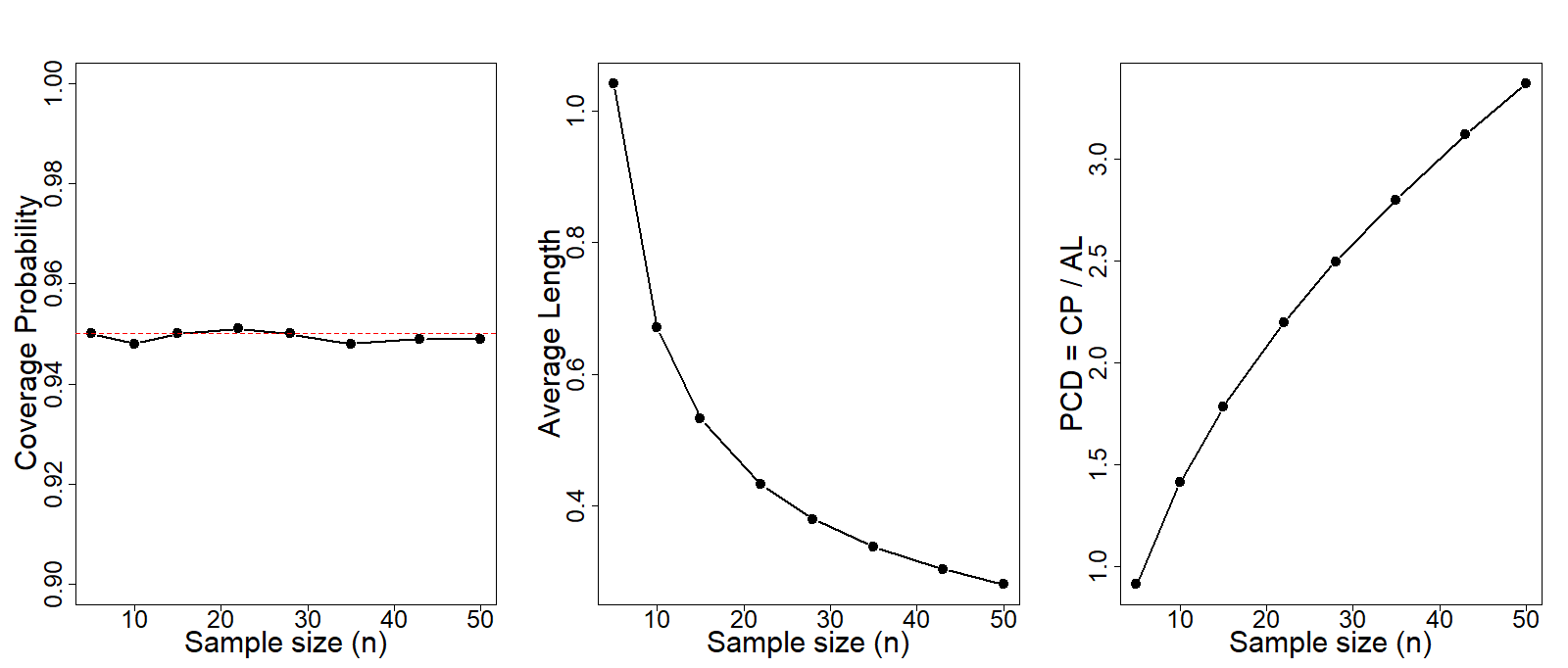
7 A simulation study : comparing the confidence intervals

In this section we will discuss the numerical performance of the derived confidence intervals of the parameter $\ln\sigma$. We use montecarlo simulation methods to compute the coverage probability (CP) and average lengths (AL). To obtain the CPs and ALs we have generated $30,000$ random samples from two normal population of sizes $n$ with equal variances $\sigma^{2}$ and means $\mu_{1}$ and $\mu_{2}$ respectively. As all the intervals location invariant and the CPS and ALs are depends on $\sigma$. Therefore, without loss of generality, we set $\mu_{1}=\mu_{2}=0$ and $\sigma=1$. In this study we have computed CP and AL for various combination of samples. For computing the bootstrap confidence intervals, the inner loop $(K)$, corresponding to the replication is taken up-to $3,000$ times. In the case of generalized confidence intervals, the inner loop is repeated $10,000$ times. Similarly, for computing the HPD credible intervals using the MCMC algorithm, we consider $10,000$ replications in the inner loop. Moreover, all the confidence intervals are computed at the significance confidence level $(1-\alpha)=0.95$. We have observed that the ALs of the bootstrap-t and bootstrap-p are equal but the CPs of the bootstrap-t intervals are greeter than the bootstrap-p intervals (see Figure 6 and 7). When we examine the performance of the confidence intervals in terms of CPs and ALs, we find that some intervals achieves the significance confidence levels $(0.95)$, but their ALs are quite large. In the other cases, some confidence intervals show their ALs are quit acceptable but their CPs are bellow the significance level. To overcome this situation, we will follow the following approaches. First we may fix a minimum acceptable confidence level for CP and consider only those intervals which achieves this level, after that we select the interval which have the smallest AL. In the second approach we consider those intervals that reach the minimum acceptable significance level and then evaluate them using a unified criterion of measure called the probability coverage density (PCD) which defined as the ratio of CP and AL. This unified criterion was proposed by [33]. This unified criterion of performance measure will take care of both quantities AL and CP at the same time. This criterion finds the intervals with lower ALs but greater CPs. It is obvious that an interval with the higher PCD value have the best performance. We have conduct the simulation study for many different sample sizes. We conclude the following observation from the Figure 5, 6, 7, 8 and 9.

Based on our simulation study we can conclude the following observation.

• All the ALs are decreasing function of $n$. The CPs are not monotonic in $n$. The values of PCD are increasing when $n$ is increasing.

• We have set a significance level at $0.95$, then bootstrap-t and the generalized confidence intervals has attain it.

• The CPs lies between $65\%$ and $95\%$. The CPs of the bootstrap-t and generalized confidence intervals are always close to 0.95.

• If we fixed the confidence level at $95\%$, the bootstrap-t and generalized confidence interval achieve this. If we adopt a more liberal confidence level of $90\%$, then all confidence intervals attain the nominal level provided that $n>20$ (approximately).

• Ranking the intervals in terms of the shortest ALs, we obtain the following order: asymptotic, HPD, bootstrap-t (or bootstrap-p) and generalized confidence intervals.

• If we rank the intervals in the basis of highest CPs, we get the following order: generalized confidence intervals, bootstrap-t, HPD, Asymptotic confidece interval and bootstrap-p confidence intervals.

• If we want to rank all the intervals in the basis of both shortest ALs and highest CPs then a clear ranking is not possible. In this challenging situation, we use the PCD criterion to select the most appropriate interval.

Figure 5: Asymptotic confidence interval

Figure 6: Bootstrap-p confidence interval

Figure 7: Bootstrap-t confidence interval

Figure 8: HPD credible interval

Figure 9: Generalized confidence interval using UMVUE

8 Real life Data analysis

In this section, we present a real-life example to illustrate the applicability of the proposed results. For data analysis, we consider failure times (in hours) of the air-conditioning systems of Boeing 720 jet planes “7907” and “7916”. Here $n=6$ (see [27]).

Table 1: Failure times (in hours) of the air-conditioning systems of two planes

Planes	Failure times (in hours)
Data 1 (Plane 7907)	194, 5, 41, 29, 33, 181
Data 2 (Plane 7916)	50, 254, 5, 283, 35, 12

Using the Kolmogorov-Smirnov test at a significance level of 0.05, we found that both datasets satisfy the normality assumption, with p-values of 0.374 and 0.405 for Data 1 and Data 2, respectively. We have checked the equality of the variances of these two datasets by F-test at the 0.05 significance level and the hypothesis $\mu_{1}\leq\mu_{2}$ was tested using the t-test at a significance level 0.05. We have obtain the values of improved estimators in Table 2. Also we have calculate values of the confidence intervals of $\ln\sigma$ in Table 3.

Table 2: Estimated values of the improved estimators of $\ln\sigma$

Loss	$\delta_{01}$	$\delta_{S}$	$\delta_{\phi_{*}}$
$L_{1}(t)~~~~~~~~~~~~~~$	4.7293	4.6768	4.6768
$L_{2}(t)\ (a_{1}=-3)$	4.8233	4.7603	4.7603
$L_{2}(t)\ (a_{1}=-2)$	4.7892	4.7303	4.7303
$L_{2}(t)\ (a_{1}=2)~~~$	4.6776	4.6300	4.6300
$L_{2}(t)\ (a_{1}=4)~~~$	4.6321	4.5882	4.5882

Table 3: Confidence intervals with lengths of $\ln\sigma$

Method	ACI	Bt	HPD	GCI
Lower	4.1864	3.9399	4.6749	3.1642
Upper	4.9865	4.8588	4.6773	4.0836
Length	0.8001	0.9188	0.0024	0.9193

9 Concluding remarks

Shannon entropy is a measure of the level of uncertainty inherent in a random phenomenon and has wide range of application in various fields such as telecommunications, meteorology, econometrics, and molecular biology. In many of these applications, data are modeled using probability distributions; thus, the estimation of entropy in a parametric framework becomes an important work. In this paper, we consider the problem pointwise and interval estimation of the entropy of two independent normal populations with unequal means. For point wise estimation, we obtain several improved estimators under a general location invariant loss function using a decision theoretic approach. In this case, we derive MLE, RMLE, an UMVUE. We also obtain a class of improved estimators that dominates the BAEE. Furthermore, by using Brewster and Zidek technique we derive a class of smooth improved estimators that also dominates BAEE. Consequently we show that the Brewster and Zidek type estimator is coincides with the Kubokawa IERD type estimator. We derive explicit expressions of the proposed improved estimators for two specific loss functions namely quadratic loss function and Linex loss function. In addition, we derive a improved estimators under generalized Pitman closeness criterion. A detailed numerical comparison of the risk performance of the estimators have been provided. In the case of interval estimation, we derive asymptotic confidence interval, bootstrap confidence intervals, generalized confidence interval, HPD credible interval using MCMC method. The interval estimators are ranked based on the lowest ALs and highest CPs in the simulation study. Finally, a real life data analysis has been conducted to illustrate the proposed results.

10 Appendix

Lemma 10.1

(Lemma $2.1$, [17]) Let $p(z)$ and $q(z)$ be positive functions such that the ratio $\dfrac{p(z)}{q(z)}$ is non-decreasing in $z$. Suppose there exists a function $r(z)$ satisfying $r(z)<0$ for $z<z^{\ast}$ and $r(z)>0$ for $z>z^{\ast}$. Then, we have

$$\int_{0}^{\infty}r(z)\,\frac{p(z)}{q(z)}\,dz\;\geq\;\frac{p(z^{\ast})}{q(z^{\ast})}\int_{0}^{\infty}r(z)\,dz.$$

Equality holds if and only if $\dfrac{p(z)}{q(z)}$ is constant almost everywhere.

Lemma 10.2

Let $d_{1}$, $d_{2}$, $n$, $\eta$ and $\alpha$ be any fixed positive real numbers with $d_{1}<d_{2}$ then the ratio of integral $\displaystyle\frac{I(y-d_{2})}{I(y-d_{1})}=\frac{\int_{-\alpha}^{\alpha}e^{-\frac{1}{4}\left(\sqrt{n}e^{y-d_{2}}w-\eta\right)^{2}}dw}{\int_{-\alpha}^{\alpha}e^{-\frac{1}{4}\left(\sqrt{n}e^{y-d_{1}}w-\eta\right)^{2}}dw}$ is increasing in $y$.

Proof: Define

$$I(y)=\int_{-\alpha}^{\alpha}e^{-\frac{1}{4}\left(\sqrt{n}e^{y}w-\eta\right)^{2}}dw.$$

By the change of variable $u=(\sqrt{n}e^{y}w-\eta)/\sqrt{2}$, we obtain,

$$I(y)= \frac{\sqrt{2}}{\sqrt{n}e^{y}}\int_{(-\sqrt{n}e^{y}\alpha-\eta)/\sqrt{2}}^{(\sqrt{n}e^{y}\alpha-\eta)/\sqrt{2}}e^{-\frac{1}{2}u^{2}}du$$

$$= \frac{2\sqrt{\pi}\left[\Phi\left(\frac{\sqrt{n}e^{y}\alpha-\eta}{\sqrt{2}}\right)-\Phi\left(\frac{-\sqrt{n}e^{y}\alpha-\eta}{\sqrt{2}}\right)\right]}{\sqrt{n}e^{y}},$$

where $\Phi$ denotes CDF of the standard normal distribution. Consider the auxiliary function

$$Q(t)=\Phi(t-\eta/\sqrt{2})-\Phi(-t-\eta/\sqrt{2}),\ t=\sqrt{n}e^{y}\alpha/\sqrt{2}$$

we may rewrite $I(y)=\tfrac{2\sqrt{\pi}}{\sqrt{n}e^{y}}Q(t)$. For fixed $d_{1}<d_{2}$, consider the ratio $R(y)=\frac{I(y-d_{2})}{I(y-d_{1})}$. Substituting the above expression yields

$$R(y)=e^{d_{2}-d_{1}}\frac{Q(t_{2})}{Q(t_{1})},$$

where $t_{1}=\sqrt{n}e^{y-d_{1}}\alpha$ and $t_{2}=\sqrt{n}e^{y-d_{2}}\alpha$. Differentiating $\log R(y)$ gives

$$\frac{d}{dx}\log R(y)=\frac{Q^{\prime}(t_{2})}{Q(t_{2})}t_{2}+\frac{Q^{\prime}(t_{1})}{Q(t_{1})}t_{1}.$$

The function $Q(t)$ is a log-concave function since it is an integral of a log-concave normal density over a symmetric interval. Hence, $\psi(t)=\frac{Q^{\prime}(t)}{Q(t)}t$ is decreasing in $t>0$. Since $d_{1}<d_{2}$, it follows that $t_{1}>t_{2}$ and therefore, $\frac{Q^{\prime}(t_{2})}{Q(t_{2})}t_{2}>\frac{Q^{\prime}(t_{1})}{Q(t_{1})}t_{1}$. Thus $\frac{d}{dx}\log R(y)>0$, which proves that $R(y)$ is strictly increasing in $y$.

Disclosure statement

No potential conflict of interest was reported by the authors.

Funding

Lakshmi Kanta Patra thanks the Anusandhan National Research Foundation, India for providing financial support to carry out this research with project number MTR/2023/000229, 02011/38/2023 NBHM (R.P)/R & DII/13409.

References

- [1] Blumenthal, S. and Cohen, A. (1968). Estimation of two ordered translation parameters, The Annals of Mathematical Statistics. 39(2), 517–530.
- [2] Brewster, J. F. and Zidek, J. (1974). Improving on equivariant estimators, The Annals of Statistics. 2(1), 21–38.
- [3] Chen, M.-H. and Shao, Q.-M. (1999). Monte carlo estimation of bayesian credible and hpd intervals, Journal of computational and Graphical Statistics. 8(1), 6992.
- [4] Chib, S. and Greenberg, E. (1995). Understanding the metropolis-hastings algorithm, The american statistician. 49(4), 327335.
- [5] Efron, B. (1982). The jackknife, the bootstrap and other resampling plans, SIAM.
- [6] Garg, N. and Misra, N. (2024). A unified study for estimation of order restricted parameters of a general bivariate model under the generalized pitman nearness criterion, Statistical Papers. 65(4), 19471983.
- [7] Golan, A., Judge, G. and Miller, D. (1997). Maximum entropy econometrics: Robust estimation with limited data. New York, BY, USA; Wiley.
- [8] Gupta, R. D. and Singh, H. (1992). Pitman nearness comparisons of estimates of two ordered normal means, Australian Journal of Statistics. 34(3), 407414.
- [9] Hall, P. and Martin, M. A. (1988). On bootstrap resampling and iteration, Biometrika. 75(4), 661671.
- [10] HASTINGS, W. (1970). Monte carlo sampling methods using markov chains and their applications, Biometrika. 57(1), 97109.
- [11] Kamavaram, S. and Goseva-Popstojanova, K. (2002). Entropy as a measure of uncertainty in software reliability, 13th Int’l Symp. Software Reliability Engineering, pp. 209210.
- [12] Kang, S.-B., Cho, Y.-S., Han, J.-T. and Kim, J. (2012). An estimation of the entropy for a double exponential distribution based on multiply type-ii censored samples, Entropy. 14(2), 161173.
- [13] Kayal, S. and Kumar, S. (2013). Estimation of the shannon’s entropy of several shifted exponential populations, Statistics & Probability Letters. 83(4), 11271135.
- [14] Kayal, S., Kumar, S. and Vellaisamy, P. (2015). Estimating the renyi entropy of several exponential populations, Brazilian Journal of Probability and Statistics. pp. 94111.
- [15] Kiefer, J. (1957). Invariance, minimax sequential estimation, and continuous time processes, The Annals of Mathematical Statistics. 28(3), 573601.
- [16] Kubokawa, T. (1991). Equivariant estimation under the pitman closeness criterion, Communications in Statistics-Theory and Methods. 20(11), 34993523.
- [17] Kubokawa, T. (1994). A unified approach to improving equivariant estimators, The Annals of Statistics. 22(1), 290–299.
- [18] Lehmann, E. L. and Romano, J. P. (2005). Testing Statistical Hypotheses (Springer Texts in Statistics), Springer.
- [19] Misra, N., Singh, H. and Demchuk, E. (2005). Estimation of the entropy of a multivariate normal distribution, Journal of multivariate analysis. 92(2), 324342.
- [20] Mitra, P. K. and Sinha, B. K. (2007). On some aspects of estimation of a common mean of two independent normal populations, Journal of statistical planning and inference. 137(1), 184193.
- [21] Mondal, S. and Patra, L. K. (2024). Improved estimation of the positive powers ordered restricted standard deviation of two normal populations, arXiv preprint arXiv:2412.05620.
- [22] Nalewajski, R. F. (2002). Applications of the information theory to problems of molecular elec tronic structure and chemical reactivity, International Journal of Molecular Sciences. 3(4), 237259.
- [23] Nayak, T. K. (1990). Estimation of location and scale parameters using generalized pitman nearness criterion, Journal of Statistical Planning and Inference. 24(2), 259268.
- [24] Patra, L. K., Kayal, S. and Kumar, S. (2020). Measuring uncertainty under prior information, IEEE Transactions on Information Theory. 66(4), 25702580.
- [25] Petropoulos, C. (2017). Estimation of the order restricted scale parameters for two populations from the lomax distribution, Metrika. 80(4), 483–502.
- [26] Pitman, E. (1991). The closest estimates of statistical parameters, Communications in Statistics Theory and Methods. 20(11), 34233437.
- [27] Proschan, F. (1963). Theoretical explanation of observed decreasing failure rate, Technometrics. 5(3), 375383.
- [28] Seo, J.-I. and Kang, S.-B. (2014). Entropy estimation of generalized half-logistic distribution (ghld) based on type-ii censored samples, Entropy. 16(1), 443454.
- [29] Seo, J.-I. and Kang, S.-B. (2015). Bayesian estimation of the entropy of the half-logistic distribution based on type-ii censored samples, International Journal of Applied Mathematics and Statistics. 53(6), 5866.
- [30] Seo, J. I. and Kim, Y. (2017). Objective bayesian entropy inference for two-parameter logistic distribution using upper record values, Entropy. 19(5), 208.
- [31] Shannon, C. E. (1948). A mathematical theory of communication, The Bell system technical journal. 27(3), 379423.
- [32] Stein, C. (1964). Inadmissibility of the usual estimator for the variance of a normal distribution with unknown mean, Annals of the Institute of Statistical Mathematics. 16(1), 155–160.
- [33] Unhapipat, S., Chen, J.-Y. and Pal, N. (2016). Small sample inferences on the sharpe ratio, American Journal of Mathematical and Management Sciences. 35(2), 105123.
- [34] Weerahandi, S. and Weerahandi, S. (1995). Generalized confidence intervals, Exact statistical methods for data analysis. pp. 143168.