TT-Sparse: Learning Sparse Rule Models with Differentiable Truth Tables

Abstract

Interpretable machine learning is essential in high-stakes domains where decision-making requires accountability, transparency, and trust. While rule-based models offer global and exact interpretability, learning rule sets that simultaneously achieve high predictive performance and low, human-understandable complexity remains challenging. To address this, we introduce TT-Sparse, a flexible neural building block that leverages differentiable truth tables as nodes to learn sparse, effective connections. A key contribution of our approach is a new soft TopK operator with straight-through estimation for learning discrete, cardinality-constrained feature selection in an end-to-end differentiable manner. Crucially, the forward pass remains sparse, enabling efficient computation and exact symbolic rule extraction. As a result, each node (and the entire model) can be transformed exactly into compact, globally interpretable DNF/CNF Boolean formulas via Quine–McCluskey minimization. Extensive empirical results across 28 datasets spanning binary, multiclass, and regression tasks show that the learned sparse rules exhibit superior predictive performance with lower complexity compared to existing state-of-the-art methods.

1 Introduction

Figure 1: AUC score against rule log-complexity scatter plot of 8 interpretable models and TabM as SOTA black-box baseline across different hyperparameters, on diabetes and heart tabular datasets.

In high-stakes deployments including healthcare, finance, public policy, and safety-critical engineering, interpretability is often a functional requirement, enabling accountability and auditability (doshi2017towards; seshia2022toward). In these regimes, post-hoc explainability methods that attempt to rationalize a black-box predictor can be brittle: the explanation may be misaligned with the true decision process (slack2020fooling; adebayo2018sanity). Rudin (Rudin2019) argues that, when possible, one should prefer inherently interpretable models over explanations of opaque ones, where transparency is a property of the model itself.

Figure 2: A TT-Sparse model trained on Heart dataset converted to Boolean decision trees, achieving 91% test ROC-AUC score and complexity of 15. The sigmoid $\sigma(\cdot)$ function is applied to the final activated weights + intercept term to obtain the probability of heart disease existence between $[0,1]$.

Rule-based predictors are a natural target for such fundamental interpretability. However, interpretability is multifaceted. First, global interpretability means that a single set of rules governs the model’s behavior for all inputs; this contrasts with local explanations that provide input-dependent rationales. Second, exact interpretability means that the extracted rules reproduce the model’s inference exactly, rather than approximately (e.g., via feature-attribution scores). In this work, we focus on the demanding but practically valuable regime of global and exact interpretability, where the entire model’s inference can be reduced to symbolic logic without approximation.

Crucially, interpretability does not guarantee human understandability. Human-subject evaluations demonstrate that cognitive load scales non-linearly; specifically, studies suggest that rule sets exceeding a complexity of 50 become functionally unintelligible (humaninterpretability). Hence, our work focuses on producing rule sets that minimize rule complexity while maintaining competitive predictive performance. Figure 1 showcases this: our model TT-Sparse achieves superior predictive performance while maintaining low rule complexity (well within the complexity threshold for human intelligibility of 50 indicated by the green region), outperforming other rule models and remaining competitive with the state-of-the-art deep tabular model, TabM (tabm).

Despite their appeal, learning high-performing rule sets while minimizing complexity remains challenging. Classical approaches often rely on discrete, heuristic search (e.g., greedy rule induction or tree growth/pruning), which can become trapped in suboptimal solutions and may struggle to exploit modern hardware efficiently (RIPPER; CART). More recent lines of work pursue global optimization objectives or neural-symbolic relaxations that enable gradient-based training, but they impose restrictive logical forms that limit expressivity (difflogicnet; petersen2024convolutional).

Truth table-based nodes offer a direct route to exact symbolic conversion via standard minimization procedures such as Quine-McCluskey (ttnet; benamira2024truth). Crucially, truth table-based nodes provide high expressivity because they are capable of representing any Boolean function over their inputs, effectively acting as the discrete counterpart to standard neural network (NN) nodes. Unlike neural-symbolic relaxations that approximate discrete logic through continuous functions, truth table nodes function as fundamental building blocks that directly map input patterns to outputs. However, making such nodes trainable at scale requires solving a key bottleneck: selecting a sparse, meaningful subset of inputs for each node in a way that remains compatible with backpropagation.

We introduce TT-Sparse, a differentiable rule-learning architecture built around Learnable Truth Table (LTT) nodes that can be transformed exactly into Boolean formulas (DNF/CNF) after training. Each LTT node learns a Boolean function over a small set of selected input features; the entire model is then a composition of these rule activations with a lightweight prediction head. The central technical challenge is that choosing which $k$ inputs feed each node is a discrete TopK operation, which is non-differentiable. TT-Sparse resolves this with a novel soft TopK operator that provides a continuous relaxation while enforcing an exact cardinality constraint in expectation, enabling stable gradient flow through the connection-selection mechanism. Concretely, we use a straight-through strategy where the forward pass uses hard TopK selections to preserve sparsity, while the backward pass uses the differentiable relaxation to update connection scores. After training, we enumerate each node’s induced truth table and apply Quine-McCluskey (quine; mccluskey) minimization to obtain compact symbolic rules, yielding global and exact interpretability.

Empirically, we evaluate TT-Sparse along the Pareto frontier of performance versus complexity. Our experiments show that TT-Sparse consistently achieves favorable trade-offs, matching or approaching the predictive performance of strong baselines while producing substantially more compact rule sets. Across a broad suite of tabular benchmarks spanning binary and multiclass classification as well as regression, TT-Sparse consistently produces competitive accuracy with markedly reduced rule complexity compared to a range of interpretable baselines, while remaining competitive to the SOTA tabular architecture.

Contributions. Hence, the main contributions of this work include: (1) We propose a novel, efficient, and fully differentiable relaxation of the discrete TopK operator, enabling end-to-end gradient-based optimization of discrete feature routing via backpropagation. (2) We introduce the TT-Sparse layer, a versatile neural building block that leverages our Soft TopK operator to dynamically learn sparse connections and extract higher-order Boolean interactions. This block is inherently flexible, allowing for seamless adaptation across diverse tasks. (3) We provide a rule extraction pipeline that converts trained LTT nodes to compact DNF/CNF rules via truth table enumeration and Quine-McCluskey minimization, leveraging data-driven don’t-care terms to reduce redundancy. We illustrate such exact rule extraction with no approximation in Figure 3. (4) Through extensive empirical validation on 28 datasets, we demonstrate that TT-Sparse establishes a new Pareto frontier in the performance-complexity landscape while achieving predictive accuracy competitive with SOTA non-pretrained tabular model, TabM.

Figure 3: Overview of the TT-Sparse Architecture. (Left) The hybrid model structure. The input vector is processed by a layer of Learnable Truth Table (LTT) nodes (blue trapezoids), which extract higher-order Boolean rules. These outputs are concatenated with the raw input features to form the final prediction. (Middle) Each potential connection is parameterized by the logic weight $W_{\text{LTT}}$ and the mapping weight $W_{\text{map}}$. Darker lines highlight the “active” connections, those where $W_{\text{map}}$ belongs to the subset of the $k$-highest mapping weights for that node. Each LTT node is convertible to an equivalent CNF/DNF equation (See Figure 4). (Right) In the forward pass, the input is fed forward and multiplied by $W_{\text{LTT}}$ if the corresponding $W_{\text{map}}$ is part of TopK. In the backward pass, gradients flow with the Soft TopK relaxation, updating both $W_{\text{map}}$ and $W_{\text{LTT}}$. This design enables exact rule extraction while preserving gradient-based training through discrete connection selection.

2 Related Work

In this section, we provide an overview of the literature on methods that achieve global and exact interpretability, as well as relaxations of the discrete TopK function. We evaluate these approaches with TT-Sparse in Section 4.

Tree-Based Approaches. While classical decision trees (CART) offer an intuitive approach, their greedy induction strategy often leads to suboptimal rule sets. To address this, GOSDT (gosdt) employs dynamic programming to find provably optimal sparse trees, though at a high computational cost for large datasets. Conversely, ensemble methods like LightGBM (lightgbm) achieve state-of-the-art predictive performance but sacrifice interpretability by distributing the decision logic across hundreds of weaker trees. However, the tree topology inherently restricts each root-to-leaf path to a logical conjunction (AND) of splitting predicates.

Heuristic-Guided Bottom-Up Rule Induction. RIPPER (RIPPER) is a classic technique that employs a greedy strategy to grow and prune rule sets, incrementally refining them to optimize predictive accuracy. Classy (classy) advances this approach by utilizing the Minimum Description Length (MDL) principle to search for compact probabilistic rule lists without the need for hyperparameter tuning. Other approaches, such as GLRM (glrm) and RuleFit (rulefit) improve scalability by leveraging column generation or tree ensembles to identify candidate rules. However, similar to the limitation with trees, these methods remain constrained by discrete heuristic generation: they build rules by iteratively adding conjunctions (ANDs), lacking the native flexibility to learn complex, nested Boolean structures (e.g., ORs) directly within a single rule unit.

Neuro-Symbolic Approaches. Neuro-symbolic models aim to combine the generalization power of neural networks with symbolic interpretability. RRL (rrl) learns a set of discrete rules by projecting logical structures into a differentiable space and applying gradient-based optimization. RL-Net (rlnet) uses a neural architecture that mimics rule lists by enforcing a hierarchical activation structure. Most recently, NeuRules (neurules) integrate feature discretization, rule construction, and rule ordering into a single end-to-end differentiable pipeline.

Differentiable TopK. Prior differentiable TopK approaches rely on iterative Optimal Transport solvers with the Sinkhorn algorithm (difftopksinkhorn; sinkhorn) or stochastic noise injection (difftopkperturb; perturb), which introduces significant computational overhead or gradient variance. Most recently, Petersen et al. (difftopkclassification) used these novel differentiable TopK operators to define a top-$k$ cross-entropy loss, enabling the direct end-to-end optimization of top-$k$ classification accuracy, achieving state-of-the-art fine-tuning results on ImageNet.

3 TT-Sparse

In this section, we introduce TT-Sparse, a Truth Table-based Sparse neural block. Each node in the TT-Sparse layer can be understood as a learnable truth table logic over its inputs, we call them Learnable Truth Table (LTT) nodes interchangeably. This block is the core interpretable unit that transforms input features into Boolean rules. Let $\vec{x}$ be the $n$-dimensional input vector to the layer, and there are $M$ LTT nodes in the layer.

There are three aspects of a TT-Sparse layer: the connection selection, the linear operation of the selected inputs, and the binarization. The connection selection mechanism leverages the soft TopK operator we introduce to enable learning by backpropagation of the loss by relaxing the discrete, non-differentiable selection of the traditional TopK.

3.1 Components

Soft TopK. First, we define the space of operators

$$S_{k}:\mathbb{R}^{n}\to\mathcal{P}_{k}\subset[0,1]^{n}$$

where $\vec{x}\in\mathbb{R}^{n}$ denotes the input vector. This space is constrained by $\sum^{n}_{i=1}S_{k}(\vec{x})_{i}=k$.

The hard TopK operator can be viewed as finding the vector $y$ within the feasible set that maximizes $x^{\top}y$, achieved by assigning the components of $y$ corresponding to the $k$ largest values of $x$ to 1, while setting the rest to 0. Since this discrete selection is not differentiable, we introduce an entropic regularizer to find a probability-like vector $\vec{y}\in[0,1]^{n}$ that is closest to the logits $\vec{x}$ (maximizing the dot product) while maintaining smoothness and summing exactly to $k$. The entropic regularizer is weighted by a predetermined parameter temperature $\tau>0$. This leads us to the optimization objective

$\vec{y}^{*}=\underset{\vec{y}\in[0,1]^{n}}{\text{argmax}}\left[\sum_{i=1}^{n}y_{i}x_{i}+\tau\sum_{i=1}^{n}H(y_{i})\right]$

subject to $\sum_{i=1}^{n}y_{i}=k$, where $H(y_{i})$ is the binary entropy $H(y_{i})=-y_{i}\log y_{i}-(1-y_{i})\log(1-y_{i})$. Solving this optimization via Lagrangian multipliers (see Appendix C), we obtain the solution $S_{k}(\vec{x}):=\vec{y}$ where $y_{i}:=\sigma(\frac{x_{i}}{\tau}+c)$ for $i\in\{1,\dots,n\}$ and $c\in\mathbb{R}$ is the unique root of $f(c)=\sum_{j=1}^{n}\sigma(\frac{x_{i}}{\tau}+c)-k=0$. Since $f(c)$ is strictly increasing, $c$ is uniquely determined and solved by the bisection method.

This formulation allows for the derivation of exact gradients with implicit differentiation. Let $s_{i}^{\prime}=\sigma^{\prime}(\frac{x_{i}}{\tau}+c)=y_{i}(1-y_{i})\text{ and }s^{\prime}=[s_{1},\dots,s_{n}]^{\top}.$

$$\frac{\partial y_{i}}{\partial x_{j}}=s^{\prime}_{i}\cdot\frac{\partial}{\partial x_{j}}\left(\frac{x_{i}}{\tau}+c\right)=\frac{1}{\tau}s^{\prime}_{i}\left(\delta_{ij}-\frac{s^{\prime}_{j}}{\|s^{\prime}\|_{1}}\right)$$ (1)

$$\nabla_{\vec{x}}S_{k}(\vec{x})=\frac{1}{\tau}\left[\text{diag}(s^{\prime})-\frac{s^{\prime}(s^{\prime\top})}{\|s^{\prime}\|_{1}}\right]$$ (2)

$$\frac{\partial y_{i}}{\partial k}=s^{\prime}_{i}\cdot\frac{\partial}{\partial k}\left(\frac{x_{i}}{\tau}+c\right)=\frac{s^{\prime}_{i}}{\|s^{\prime}\|_{1}}$$ (3)

$$\nabla_{k}S_{k}(\vec{x})=\frac{s^{\prime}}{\|s^{\prime}\|_{1}}$$ (4)

The complete derivation of the partials can be found in Section C.2. Notice that the gradient is scaled by the inverse temperature $\frac{1}{\tau}$, similar to the effect of temperature in the softmax function when approximating the Heaviside step function. As $\tau\to 0$, the relaxation gets closer to the hard, discrete counterpart. The effect of temperature $\tau$ on the distribution of probabilities is illustrated in Figure 6.

In the implementation of the bisection search of $c$, it takes around 25 halving iterations before reaching machine precision limits of float32 ($\epsilon\approx 10^{-6})$, taking around 1 ms to complete for a batch of 16 input vectors. See Section C.4 for visualization of the convergence of the bisection method.

LTT Nodes. Let $\vec{x}\in\mathbb{R}^{n}$ denote the input to the TT-Sparse layer with $M$ LTT nodes. The block has 2 learnable modules: the connection mapping represented by a matrix $W_{\text{map}}\in\mathbb{R}^{n\times M}$ and the truth table logic represented by matrix $W_{\text{LTT}}\in\mathbb{R}^{n\times M}$ (augmented by a bias vector $b\in\mathbb{R}^{M}$).

For each LTT node $j\in\{1,\dots,M\}$, the objective is to select a sparse subset of $k$ input features to form a truth table of size $2^{k}$ and learn effective truth table logic over the features. To determine the active inputs for node $j$, we define a selection mask vector $m^{(j)}\in\{0,1\}^{n}$.

In the forward pass, this mask is discrete. It selects the indices corresponding to the top-$k$ values in the $j$-th column of the mapping matrix:

$$m^{(j)}_{\text{forward},i}=\begin{cases}1&\text{if }W_{\text{map}}[i,j]\in\text{TopK}(W_{\text{map}}[:,j])\\ 0&\text{otherwise}\end{cases}$$

for $i\in[1,\dots,n]$.

The output of each LTT node is the linear combination of the active features

$$z_{j}(\vec{x})=\sum_{i=1}^{n}m_{i}^{(j)}\cdot W_{\text{LTT}}[i,j]\cdot x_{i}+b_{j}$$ (5)

However, the traditional TopK operation is discrete and not differentiable, so without relaxation, the connection matrix will not update to find better connections for the LTT logic. Thus, we leverage the soft TopK operator $S_{k}$ we propose in 3.1 to replace $m^{(j)}$ in the backward pass to:

$$m^{(j)}_{\text{backward}}=S_{k}(W_{\text{map}}[\cdot,j])$$

Consequently, the partial derivatives w.r.t. the connection weights are computed via the chain rule. Let $\delta_{j}=\frac{\partial\mathcal{L}}{\partial z_{j}}$ be the gradient of the loss function $\mathcal{L}$ w.r.t. the node output $z_{j}$. The gradient flow to the connection matrix is given by

$$\frac{\partial\mathcal{L}}{\partial W_{\text{map}}[\cdot,j]}=\frac{\partial\mathcal{L}}{\partial z_{j}}\cdot\frac{\partial z_{j}}{\partial m^{(j)}_{\text{backward}}}\cdot\frac{\partial S_{k}(W_{\text{map}}[\cdot,j])}{\partial W_{\text{map}}[\cdot,j]}$$ (6)

The term $\frac{\partial z_{j}}{\partial m^{(j)}_{\text{backward}}}$ is an $n$-dimensional vector representing the potential contribution of each feature if selected, given by

$$\frac{\partial z_{j}}{\partial m^{(j)}_{\text{backward}}}=\vec{x}\odot W_{\text{LTT}}[\cdot,j]$$

The term $\frac{\partial S_{k}(W_{\text{map}}[\cdot,j])}{\partial W_{\text{map}}[\cdot,j]}$ is the Jacobian of the Soft TopK operator, $J_{S_{k}}\in\mathbb{R}^{n\times n}$ given by equation (2). The full derivation of the gradient is provided in Appendix D. This mechanism allows the TT-Sparse layer to dynamically re-route connections into the LTT node while learning the LTT logic during training.

Finally, to function as a Boolean logic gate, the continuous output $z_{j}$ is binarized. Differentiability is maintained with a straight-through estimator (STE): $y_{j}=\mathbf{1}_{(z_{j}>0)}+(z_{j}-\text{stop\_gradient}(z_{j}))$.

3.2 TT-Sparse Design

The architecture of the overall model is designed as a hybrid neural block that integrates high-order feature interaction logic through the TT-Sparse layer with linear single-order features.

The layer processes an $n$-dimensional input vector $\vec{x}$ to produce $M$ binary rule activations $\vec{z}\in\{0,1\}^{M}$ via the LTT nodes. Then, we implement a skip-concatenation, so the final representation $\vec{h}$ is formed by concatenating the raw input features with the LTT rule outputs: $\vec{h}=[\vec{x}\parallel\vec{z}]\in\mathbb{R}^{n+M}$. This combined vector is then fed into a final classifier or regressor layer $f_{\text{cls}}(\vec{h})=\sigma(W_{\text{cls}}\vec{h}+b_{\text{cls}})$, depending on the task (binary/multiclass/regression). The final linear classifier layer assigns weights to both the higher-order and single-order rules, before the task-specific activation function.

While the TT-Sparse layer selects several inputs per node, not all connections or all nodes may be essential for a given task. To identify the most compact and effective rule set, we implement a post-hoc iterative magnitude pruning after the initial training phase. Connections in the TT-Sparse layer are removed based on the weights’ $L_{1}$ norm, followed by an iterative fine-tuning of the non-zeroed weights. Throughout this refinement process, the selected connections of the LTT nodes remain fixed to the selected indices by $W_{\text{map}}$ during training. This refinement phase focuses on optimizing the weights of the established logical structure, finding the lightest and most effective rule logic for the given task.

3.3 Rule Extraction

Each node $j$ in the TT-Sparse layer represents a learnable Boolean logic of its selected inputs. Let $\mathcal{I}_{j}\subset\{1,\dots,n\}$ be the selected indices of the input features by the TopK operator on $W_{\text{map}}$, where $|\mathcal{I}_{j}|=k$. Recall that the output of the node $z_{j}(\vec{x})$ is determined by the thresholded linear combination of the inputs as in Equation (5).

To extract the explicit Boolean formula of the input features for node $j$, we perform a simple truth table enumeration. All $2^{k}$ possible binary inputs are efficiently iterated and for each input, the node’s output activation is computed, obtaining the truth table $\mathcal{T}_{j}$ for node $j$

$$\mathcal{T}_{j}=\{(v_{i},z_{j}(v_{i}))|v_{i}\in\{0,1\}^{k}\}_{i=1}^{2^{k}}$$

where $v_{i}$ denotes the $i$-th binary vector in the enumeration of the input space. The subset of the truth table where the output is 1, i.e. $\mathcal{M}_{j}=\{v_{i}\in\{0,1\}^{k}\mid z_{j}(v_{i})=1\}$, are the minterms of the Boolean function.

Figure 4: Conversion of an LTT node to DNF by truth table enumeration of $2^{n}$ input combinations and obtaining the binary outputs with the LTT weight and bias parameters.

To minimize rule complexity, we identify Don’t-Care Terms (DCTs)—input combinations ($v_{i}$) that do not appear in the training data. Following the identification of minterms and DCTs, the truth table is synthesized into a CNF or DNF expression via the Quine-McCluskey (QMC) algorithm (quine; mccluskey) (Algorithm 1). By optimally assigning binary values to these DCTs, the algorithm minimizes the resulting rule complexity while maintaining exact fidelity on the observed training distribution.

Table 1: Binary Classification Results: AUC $\uparrow$ (top) and Complexity $\downarrow$ (bottom) for each dataset. Standard error in subscript. Best values in bold. The last row reports the avg. rank $\downarrow$ of each model’s AUC across all datasets, as calculated for the Friedman statistical test. OOM indicates out-of-memory during training.

Dataset	TT-Sparse	GOSDT	GLRM	RuleFit	Classy	NeuRules	RL-Net	RRL	DWN	TabM
bank	.9096.00	.6662.01	.8928.00	.8963.01	.9042.00	.8648.01	.6917.01	.8913.01	.8480.01	.9351.00
	11237	50	382	5820	37013	90245	13186	737	53331	-
blood	.7554.02	.6155.04	.7093.05	.7059.05	.6628.03	.7116.02	.5618.05	.6712.04	.6545.05	.7193.04
	158	155	305	437	92	1653	2010	52	46529	-
calhousing	.9307.00	.8111.01	.9205.01	.9259.00	.9072.01	.8804.01	.8004.03	.8684.01	.7961.01	.9667.00
	6211	250	1087	13146	45717	2298	881	453	57221	-
compas	.7301.01	.6765.01	.7236.01	.7270.01	.7080.01	.7129.01	.6851.02	.6825.01	.6629.01	.7311.01
	92	130	384	3116	392	2806	9611	175	135828	-
covertype	.8554.00	OOM	.8437.00	.8465.00	.8913.00	.8320.00	.7672.01	.8522.00	.8002.00	.9801.00
	19431		491	396	2183102	28428	19416	3258	46416	-
cc_default	.7915.01	.7011.01	.7705.01	.7802.00	.7631.01	.7596.01	.7233.00	.7454.02	.6601.02	.7883.01
	12819	62	5624	11041	1163	28120	4402	10020	44518	-
creditg	.7919.04	.5788.02	.6851.04	.7948.04	.6768.02	.7313.05	.6625.04	.6745.05	.7234.07	.7329.03
	5436	276	565	9724	132	781148	2460	358	244436	-
diabetes	.8208.02	.6443.03	.7796.02	.8024.01	.7260.02	.6854.05	.6442.02	.7609.03	.7186.04	.7957.01
	149	52	8710	197	143	181	910	247	58826	-
electricity	.8823.00	.7734.00	.8705.00	.8745.00	.8895.00	.8397.01	.7459.01	.8387.01	.8160.00	.9666.00
	9929	200	613	18632	73112	2406	11210	566	291396	-
eye	.6312.02	.5836.00	.6278.01	.6216.01	.5913.02	.5981.01	.5815.01	.5930.01	.5711.02	.6799.02
	7643	82	162	4618	386	71524	19210	6411	34019	-
heart	.9308.01	.8140.01	.9149.02	.9151.01	.8749.01	.8663.01	.8301.01	.8661.03	.8719.02	.9236.02
	1115	20	396	3416	312	1009	6410	2910	47420	-
income	.9147.00	.7341.01	.8958.00	.9121.00	.8799.00	.8800.01	.7707.02	.8962.01	.8642.01	.9230.00
	15240	112	282	15547	68422	41358	43451351	30718	104523	-
jungle	.8917.00	.7804.01	.8904.00	.8630.01	.9476.00	.8702.01	.7685.03	.8781.01	.7900.01	.9970.00
	26275	274	514	10348	89125	1631	4210	284	44025	-
road_safety	.7764.00	.7197.01	.7603.00	OOM	.8435.00	.7842.01	.7465.01	.8293.01	.7295.02	.8852.01
	23654	158	241		134833	1869	194838	11910	42513	-
Avg. rank $\downarrow$	1.53	8.27	3.6	3.07	3.8	4.8	7.93	4.87	7.13

By modeling the node truth table logic as a thresholded linear combination of the selected inputs, TT-Sparse requires only $n+1$ learnable parameters (one weight per selected input plus a bias term) to represent the logic, a linear complexity compared to DiffLogicNet (difflogicnet) double-exponential and DWN (dwn) exponential complexities.

DiffLogicNet introduces a differentiable relaxation of the Boolean logic to implement binary gates as nodes, by learning a probability distribution over the set of all possible binary operators for a given number of inputs. While effective for 2-input gates, this approach scales poorly as the number of possible Boolean functions grows double exponentially with the number of inputs, $(2^{2^{n}})$.

Table 2: Multiclass Classification Results: AUC $\uparrow$ (top) and Complexity $\downarrow$ (bottom) for each dataset. Standard error in subscript. Best values in bold. The last row reports the avg. rank $\downarrow$ of each model’s AUC across all datasets, as calculated for the Friedman statistical test.

Dataset	TT-Sparse	GOSDT	Classy	NeuRules	RL-Net	DWN	TabM
car	.9901.00	.6636.03	.9727.01	.8930.02	.8631.03	.6967.06	1.0000.00
	252110	4112	1366	22711	736	244563	-
ecoli	.9663.01	.8315.05	.8968.02	.9340.01	.7551.05	.8841.02	.9629.01
	14877	164	344	2013	360	13583	-
iris	.9993.00	.9500.02	.9633.02	.9883.01	.9040.05	.8090.04	.9963.01
	2617	72	120	251	3010	240668	-
penguins	1.0000.00	.9519.03	.9795.02	.9893.01	.9551.02	.9503.02	.9998.00
	61	152	193	2128	502	106555	-
satimage	.9802.00	.8408.01	.9587.00	.9488.01	.8094.03	.8652.02	.9925.00
	15718	173	40812	3789	7402	55426	-
wine	1.0000.00	.9592.01	.9430.03	.9807.02	.9543.06	.9528.01	1.0000.00
	72	163	130	956	11210	79521	-
yeast	.8457.02	.6767.02	.7809.02	.7787.01	.7082.03	.6721.04	.8564.02
	7714	376	13511	3078	425	305041	-
Avg. rank $\downarrow$	1	4.71	3	2.43	4.71	5.14

The DWN model addresses this scalability bottleneck by parameterizing nodes as Lookup Tables (LUTs) and introducing an Extended Finite Difference method to estimate gradients. This reduces the parameter complexity from $2^{2^{n}}$ to $2^{n}$, the size of the lookup table itself. However, by parameterizing a regular lookup table, a standard LUT is strictly position-dependent; the meaning of its weights is tied to the specific ordering of its address. If the input selection mechanism permutes the selected features (e.g. swapping index $i$ with index $j$), the LUT weights do not accommodate this shift, causing performance inefficiency. In contrast, the TT-Sparse node uses a linear combination of the inputs, which is commutative, making the node robust to input reordering during the connection search phase.

Pruning a single input connection from a dense LUT is also non-trivial. To make a LUT invariant to a specific input bit, one must constrain half of the table’s parameters to be identical to the other half (based on Shannon expansion). In the TT-Sparse formulation, removal of a redundant input connection can simply be done by pushing the corresponding linear weight to zero via $L_{1}$ norm.

We validate these theoretical advantages by replacing the TT-Sparse block in our model with the DWN block in our experimental evaluation (Tables 1-3).

4 Experiments

In this section, we validate the efficacy of TT-Sparse across the 3 main tabular tasks: binary and multiclass classification, and regression. Our evaluation aims to answer 2 fundamental questions: (1) Can TT-Sparse generate rule sets that are Pareto-competitive, offering a better trade-off between predictive performance and complexity compared to existing interpretable models? (2) How does the performance of TT-Sparse compare to TabM (tabm), the current state-of-the-art non-pretrained deep learning architecture for tabular data? The code for this project is publicly available at .

Datasets and Tasks. We conduct experiments on 28 datasets (14 binary, 7 multiclass, 7 regression). We evaluate the Area Under the Receiver Operating Characteristic Curve (ROC-AUC) score for the binary and multiclass (One-vs-Rest) classification to judge predictive performance while handling class imbalance. For regression tasks, we evaluate the $\mathbf{R^{2}}$ score.

Baselines. We compare TT-Sparse against the interpretable baselines we discussed on the Related Work (section 2): GOSDT (gosdt), GLRM (glrm), RuleFit (rulefit), Classy (classy), NeuRules (neurules), RL-Net (rlnet), RRL (rrl), and DWN (dwn).

Our objective is to maximize predictive performance (AUC/$R^{2}$) while minimizing rule complexity. The complexity of a rule set is simply defined as the sum of the number of rules and the number of Boolean operators in all the rules. Crucially, for multiclass tasks, we calculate a single global complexity score: a rule or feature contributes to the complexity count exactly once if it holds a non-zero weight for any target class, ensuring that logic shared across classes is not penalized multiple times. Refer to Appendix F for examples of rules generated by each interpretable model and its complexity. Because the output of a rule-based model depends on its hyperparameters, a single performance number does not provide a complete picture. For comprehensive evaluation, we visualize the performance complexity Pareto frontier for every model on every dataset (see Appendix E). The results presented in Tables 1, 2, and 3 report the performance of the model configuration that achieves the best performance-complexity of this Pareto grid. Due to architectural limitations, GLRM and RuleFit cannot handle multiclass classification, and the remaining models are limited to classification.

Table 3: Regression Results: $R^{2}\uparrow$ (top) and Complexity $\downarrow$ (bottom) for each dataset. Standard error in subscript. Best values in bold. The last row reports the avg. rank $\downarrow$ of each model’s $R^{2}$ across all datasets, as calculated for the Friedman statistical test.

Dataset	TT-Sparse	GLRM	RuleFit	TabM
abalone	.5328.01	.4103.02	.5324.01	.5494.02
	4316	536	237	-
bike	.6956.01	.1879.05	.7380.01	.9547.00
	29921	505	12727	-
boston	.8566.01	.6541.10	.8576.05	.9042.01
	7741	7414	8917	-
california	.7102.01	.5473.04	.7006.01	.8432.01
	13530	19720	10134	-
crime	.3647.08	.4893.04	.6540.01	.6513.02
	300322	685	7933	-
parkinsons	.9232.01	.8598.02	.9270.01	.9909.00
	10390	966	8215	-
wine_reg	.3121.02	.2151.04	.3090.03	.3629.10
	11146	598	8521	-
Avg. rank $\downarrow$	1.71	2.86	1.43

For all binary classification datasets except covertype, jungle, and road_safety (Table 1), TT-Sparse consistently pushes the Pareto limit, achieving comparable or better performance with lower complexity. While GOSDT often yields the lowest complexity rules with sparse decision trees, it frequently suffers from performance issues. For some datasets (blood, compas, cc_default, creditg, diabetes, heart, income), TT-Sparse remains competitive with the SOTA DL baseline TabM, notably surpassing it on the Heart dataset with low complexity.

Multiclass classification (Table 2) highlights the strongest advantage of our approach. With GLRM and RuleFit unable to operate in this setting, TT-Sparse comfortably outperforms the other models in all datasets as the Pareto frontier, and is very close to achieving TabM performance while maintaining full transparency. TT-Sparse also shows strong competitiveness for the regression tasks (Table 3), effectively outperforming GLRM and underperforming RuleFit in rank by a thin margin.

4.1 Ablation Study

A core contribution of TT-Sparse is the use of the Soft TopK operator to select the input connections for each LTT node. To validate the necessity and efficiency of this design, we perform an ablation study comparing it against a baseline connection selection mechanism leveraging the softmax operator as a relaxation of the argmax operator, used in DWN (dwn).

Baseline. In the baseline configuration we ablate against, instead of selecting $k$ features from a single importance vector, the $k$ inputs to a truth table are treated as distinct, ordered ”slots”. Mathematically, the connection matrix for the layer is $W_{\text{map}}\in\mathbb{R}^{n\times kM}$ instead of $W_{\text{map}}\in\mathbb{R}^{n\times M}$. For each node $j$ in the layer, the $k$ inputs to the node are determined by taking an argmax over $k$ columns in the matrix, and, in the backpropagation, the weights are updated by taking the relaxation of argmax with softmax.

This baseline exhibits two disadvantages relative to our proposed soft TopK approach: (1) Parameter inefficiency, where mapping complexity scales as $\mathcal{O}(M\cdot n\cdot k)$ rather than $\mathcal{O}(M\cdot n)$; and (2) Input redundancy, where independent slots may converge on the same feature index, effectively collapsing the dimension of the truth table. Our soft TopK operator inherently prevents this by selecting the $k$ most relevant distinct indices from the columns of the mapping matrix.

Experimental results (Figure 5) demonstrate that TT-Sparse (x-axis) consistently yields superior predictive performance compared to the Softmax baseline (y-axis).

Figure 5: Predictive performance comparison (AUC/$R^{2}$, higher is better) between TT-Sparse (Soft TopK) and the slot-based Softmax baseline. Points below the diagonal indicate superior performance by TT-Sparse.

5 Conclusion

In this work, we introduced TT-Sparse, a new neural building block designed to achieve highly performant rule sets while minimizing complexity. By reformulating truth tables as differentiable modules with sparse connectivity learned through the new soft TopK operator, we enable the end-to-end learning of Boolean logic via standard gradient descent. Furthermore, as a fully differentiable layer, TT-Sparse offers significant architectural flexibility; it can be seamlessly integrated into standard neural pipelines to learn interpretable rules across diverse problem settings, including binary, multiclass, and regression tasks.

5.1 Limitations

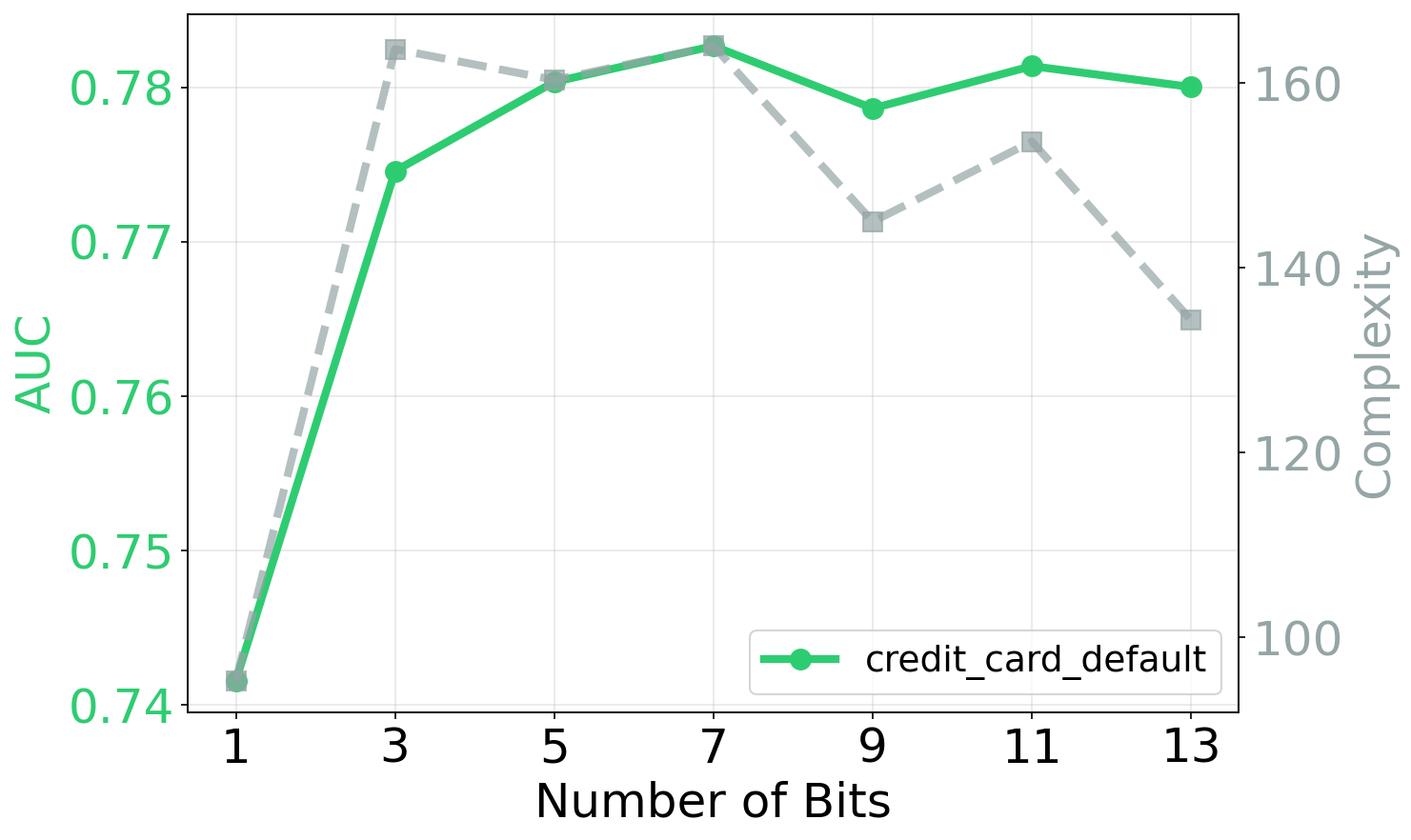
Continuous features must be encoded before training, fixing the representation of the literals. Second, the utilization of the soft TopK operator makes training reliant on the initialization of the temperature parameter $\tau$. While these parameters must be well-initialized, our ablations in Appendix H show that TT-Sparse is robust to this constraint, maintaining high performance after as few as 5 encoding bits.

5.2 Future Work

Future research will focus on enhancing the architectural expressivity of TT-Sparse for broader data domains. We aim to adapt the LTT nodes for time-series analysis by introducing recurrent latent dimensions, enabling the Soft TopK operator to sparsely select historical states and extract interpretable temporal logic. Additionally, we plan to extend the feature selection mechanism to support literals formed by learnable linear combinations of input variables (e.g. $w_{1}x_{1}+w_{2}x_{2}\leq z$) to capture complex decision boundaries, thereby reducing the Boolean complexity required to approximate non-linear functions.

6 Impact Statement

This work advances the field of interpretable machine learning by introducing a scalable framework for achieving global and exact interpretability without sacrificing predictive performance. This directly addresses the transparency requirements of high-stakes sectors such as healthcare, finance, and criminal justice, where auditability and accountability are essential. By enabling domain experts to inspect, verify, and reason about model behavior, TT-Sparse facilitates algorithmic oversight, strengthens institutional trust, and supports informed, responsible use of machine-learning systems under emerging regulatory frameworks.

Appendix A Datasets

We benchmark with 28 publicly available datasets (14 binary, 7 multiclass, 7 regression) used in prior works (neurules; whydotree; tabarena; glrm; tabllm).

Table 4: Dataset information: the tabular task, the dataset name, the number of rows, the number of continuous columns, categorical columns, the number of instances per class for binary and multiclass datasets.

Task	Dataset	# Rows	# Cont.	# Cat.	Classes
Binary	bank	45,210	8	8	39921/5289
	blood	748	4	0	570/178
	calhousing	20,640	8	0	10323/10317
	compas	4,966	3	8	2483/2483
	covertype	423,680	10	44	211840/211840
	credit_card_default	13,272	20	1	6636/6636
	creditg	1,000	7	13	300/700
	diabetes	768	8	0	500/268
	electricity	38,474	7	1	19237/19237
	eye_movements	7,608	20	3	3804/3804
	heart	918	5	6	410/508
	income	48,842	6	8	37155/11687
	jungle	44,819	6	0	21757/23062
	road_safety	111,762	29	3	55881/55881
Multiclass	car	1,728	0	6	1210/384/69/65
	ecoli	327	5	2	143/77/35/20/52
	iris	150	4	0	50/50/50
	penguins	333	4	3	146/68/119
	satimage	6,435	36	0	1533/703/1358/626/707/1508
	wine	178	13	0	59/71/48
	yeast	1,479	6	2	244/429/463/44/35/51/163/30/20
Regression	abalone	4,177	7	1	-
	bike	17,379	4	8	-
	boston	506	11	2	-
	california	20,640	8	0	-
	crime	1,994	122	5	-
	parkinsons	5,875	19	1	-
	wine_reg	6,497	11	0	-

Appendix B Implementation Details

B.1 Hardware

For all experiments, we use 4 Nvidia GeForce RTX 3090 GPUs and 48 cores Intel(R) Core(TM) i7-8650U CPU clocked at 1.90 GHz, 16 GB RAM. The hardware chosen was based on availability; neural networks under PyTorch (TT-Sparse, NeuRules, RL-Net, RRL, DWN, TabM) were run on GPU, while tree-based model GOSDT and rule induction based models (Classy, GLRM, RuleFit) were run on CPU.

B.2 Hyperparameters and Training Protocol

For each dataset, we reserve 20% of the data as a hold-out test set using a fixed seed. The remaining 80% is used for hyperparameter tuning. We perform a grid search by further splitting this development set into 80% training and 20% validation. Once the optimal hyperparameters are identified based on the validation metric (AUC for classification, $R^{2}$ for regression), we retrain the model on the full development set. This process is repeated across 5 different random seeds and we report the model’s performance on the hold-out test set.

We tune the key hyperparameters for all models by performing GridSearch:

• TT-Sparse: Number of bits $\in\{4,5,6\}$, Number of LTT nodes $\in\{1,20,30,40,50\}$, Soft TopK temperature $\tau\in\{0.001,0.01,0.05\}$.

• RuleFit: max_rules $\in\{5,20,40,60,80\}$ and regularization strength $Cs\in\{1,5,10,50\}$.

• GLRM: Regularization penalty $\lambda_{0}\in\{0.05,0.01,0.005\}$. We fix $\lambda_{1}=0.2\cdot\lambda_{0}$ as per (glrm).

• Classy (MDL-Rule-List): min_support $\in\{5,10,15,20,30\}$, maximum depth $\in\{3,5,7\}$, and number of cutpoints $\in\{5,7\}$.

• GOSDT: Regularization parameter $\in\{0.005,0.01,0.05\}$ and depth budget $\in\{3,5,7\}$.

• NeuRules: n_rules $\in\{5,10,20,40,60,80\}$, predicate temperature $\in\{0.1,0.2\}$, and selector temperature $\in\{0.5,1.0\}$.

• RL-Net: n_rules $\in\{5,10,20,40,60,80\}$, conjunction penalty $\lambda_{and}\in\{0.01,0.005,0.001\}$, and $L_{2}$ regularization $\in\{0,0.001,0.01\}$.

• DWN (Linear): Hidden layer sizes $\in\{20,30,40,50\}$ and Look-Up Table (LUT) size $\in\{4,5,6\}$. To ensure a fair comparison with TT-Sparse, we implemented the classifier layer immediately following the LUT layer. This architecture introduces a linear operation by assigning a weight to each LUT and adding a bias term before the activation function. The logic rules are derived similarly as TT-Sparse, utilizing Quine-McCluskey conversion to transform LUT minterms into DNF equations.

• TabM: We use the AdamW optimizer and a batch size of 512. Number of layers $\in\{1,2,3\}$, hidden size $\in\{64,128,256,512\}$, dropout rate $\in\{0,0.1,0.2\}$, learning rate $\in\{0.01,0.005,0.001\}$, bin count for embeddings $\in\{8,16,32,64\}$, and embedding dimension $\in\{8,16,32,64\}$.

Appendix C Soft TopK

Figure 6: The output distribution of the soft TopK operator with $k=3$ applied on input vector $[-2.2,0.3,0.4,1.4,10]$ across different temperatures $\tau$. $y$-axis represents the output mass for each index of the input vector.

$S_{k}(\vec{x})=[y_{1},\dots,y_{n}]$ where $y_{i}=\sigma(\frac{x_{i}}{\tau}+c)$, constrained by $\sum_{j=1}^{n}\sigma(\frac{x_{i}}{\tau}+c)=k$. $\sigma(x)=\frac{1}{1+e^{-x}}$ is the sigmoid function and $\sigma^{\prime}(x)=\sigma(x)(1-\sigma(x))$. Let $s_{i}^{\prime}=\sigma^{\prime}(\frac{x_{i}}{\tau}+c)=\frac{d}{d(\frac{x_{i}}{\tau}+c)}\sigma(\frac{x_{i}}{\tau}+c)=y_{i}(1-y_{i})\text{ and }s^{\prime}=[s_{1},\dots,s_{n}]^{\top}$.

C.1 Solving the optimization objective via Lagrangian multipliers

Recall the optimization objective

$$\vec{y}^{*}=\underset{\vec{y}\in[0,1]^{n}}{\text{argmax}}\left[\sum_{i=1}^{n}y_{i}x_{i}+\tau\sum_{i=1}^{n}H(y_{i})\right]\text{ subject to }\sum_{i=1}^{n}y_{i}=k$$ (7)

where $H(y_{i})$ is the binary entropy $H(y_{i})=-y_{i}\log y_{i}-(1-y_{i})\log(1-y_{i})$. We then derive the optimum by introducing a Lagrange multiplier $\lambda$ for the $\sum_{i=1}^{n}y_{i}=k$ constraint such that the problem becomes

$$\mathcal{L}(\vec{y},\lambda) =\sum_{i=1}^{n}y_{i}x_{i}+\tau\sum_{i=1}^{n}\bigg(-y_{i}\log y_{i}-(1-y_{i})\log(1-y_{i})\bigg)-\lambda\left(\sum_{i=1}^{n}y_{i}-k\right)$$ (8)

$$\frac{\partial\mathcal{L}}{\partial y_{i}} =x_{i}+\tau\left(\log\frac{1-y_{i}}{y_{i}}\right)-\lambda=0$$ (9)

Setting the derivative 0, we obtain the solution $y_{i}=\frac{1}{1+e^{-}\frac{(x_{i}-\lambda)}{\tau}}=\sigma(\frac{x_{i}-\lambda}{\tau})$, where $\sigma(\cdot)$ is the sigmoid function. Thus, setting $c=-\frac{\lambda}{\tau}$, we define $S_{k}(\vec{x}):=\vec{y}$ where $y_{i}:=\sigma(\frac{x_{i}}{\tau}+c)$ for $i\in\{1,\dots,n\}$ and $c\in\mathbb{R}$ is the unique root of $f(c)=\sum_{j=1}^{n}\sigma(\frac{x_{i}}{\tau}+c)-k=0$. Since $f(c)$ is strictly increasing, $c$ is uniquely determined and solved by the bisection method.

C.2 Obtaining $\nabla_{\vec{x}}S_{k}(\vec{x})$

We want the Jacobian $J\in R^{n\times n}$ where $J_{ij}=\frac{\partial y_{i}}{\partial x_{j}}$.

First, we apply the chain rule to $y_{i}=\sigma(\frac{x_{i}}{\tau}+c)$:

$$\frac{\partial y_{i}}{\partial x_{j}}=\sigma^{\prime}\left(\frac{x_{i}}{\tau}+c\right)\cdot\frac{\partial}{\partial x_{j}}\left(\frac{x_{i}}{\tau}+c\right)$$

Since $\frac{\partial x_{i}}{\partial x_{j}}=\delta_{ij}$:

$$\frac{\partial y_{i}}{\partial x_{j}}=s^{\prime}_{i}\left(\frac{1}{\tau}\delta_{ij}+\frac{\partial c}{\partial x_{j}}\right)$$ (10)

where $\delta_{ij}=\mathbf{1}_{\{i=j\}}$ is the Kronecker delta. Next, we differentiate the constraint function w.r.t. $x_{j}$ to obtain:

$$\frac{\partial}{\partial x_{j}}\sum_{m=1}^{n}\sigma\left(\frac{x_{m}}{\tau}+c\right) =0.$$ (11)

$$\sum_{m=1}^{n}s^{\prime}_{m}\left(\frac{1}{\tau}\delta_{mj}+\frac{\partial c}{\partial x_{j}}\right) =0.$$ (12)

$$\frac{1}{\tau}s^{\prime}_{j}+\left(\sum_{m=1}^{n}s^{\prime}_{m}\right)\frac{\partial c}{\partial x_{j}} =0.$$ (13)

$$\frac{\partial c}{\partial x_{j}} =-\frac{1}{\tau}\frac{s^{\prime}_{j}}{\|s^{\prime}\|_{1}}$$ (14)

Substituting this back to Equation (1):

$$\frac{\partial y_{i}}{\partial x_{j}} =\frac{1}{\tau}s^{\prime}_{i}\left(\delta_{ij}-\frac{s^{\prime}_{j}}{\|s^{\prime}\|_{1}}\right)$$ (15)

$$\nabla_{\vec{x}}S_{k}(\vec{x}) =\frac{1}{\tau}\left[\text{diag}(s^{\prime})-\frac{s^{\prime}(s^{\prime})^{\top}}{\|s^{\prime}\|_{1}}\right]$$ (16)

C.3 Obtaining $\nabla_{k}S_{k}(\vec{x})$

$$\frac{\partial y_{i}}{\partial k} =s^{\prime}_{i}\cdot\frac{\partial}{\partial k}\left(\frac{x_{i}}{\tau}+c\right)$$ (17)

$$\frac{\partial y_{i}}{\partial k} =s^{\prime}_{i}\cdot\frac{\partial c}{\partial k}$$ (18)

Then, similarly, we differentiate both sides of the constraint function w.r.t. $k$ to obtain:

$$\frac{\partial}{\partial k}\sum_{m=1}^{n}\sigma\left(\frac{x_{m}}{\tau}+c\right) =1$$ (19)

$$\sum_{m=1}^{n}s^{\prime}_{m}\cdot\frac{\partial c}{\partial k} =1$$ (20)

$$\frac{\partial c}{\partial k} =\frac{1}{\|s^{\prime}\|_{1}}$$ (21)

Substituting this back to Equation (9):

$$\frac{\partial y_{i}}{\partial k} =\frac{s^{\prime}_{i}}{\|s^{\prime}\|_{1}}$$ (22)

$$\nabla_{k}S_{k}(\vec{x}) =\frac{s^{\prime}}{\|s^{\prime}\|_{1}}$$ (23)

C.4 Convergence of bisection method

Figure 7: Absolute error $|\sum y_{i}-k|$ (log scale) vs. iterations for a batch of 16-input vectors $\vec{x}\in\mathbb{R}^{100}$ with target $k=10$. Each light blue line represents the error plot of an input vector in the batch.

To compute the constant $c$, we implement vectorized bisection search that solves for $c$ across an entire batch simultaneously on GPU. The bisection method halves the search space in every iteration, so the absolute error $|\sum S_{k}(\vec{x})_{i}-k|$ decays with $\epsilon_{t}\propto 2^{-t}$.

Figure 7 illustrates the convergence of this method. The soft TopK is applied to a batch of 16 input vectors $\vec{x}\in\mathbb{R}^{100}$ with target $k=10$. The theoretical linear convergence (linear slope on the semi-log plot) is observed empirically. The error magnitude drops below $10^{-3}$ within 15 iterations and reaches the limit of Float32 machine precision in around 30 iterations. Our experiments also show negligible overhead with around 1 ms for a batch of size 16, giving a throughput of more than 10000 samples per second.

Appendix D TT-Sparse Parameter Gradients

Let $\vec{x}\in\mathbb{R}^{n}$ denote the input to the TT-Sparse layer with $M$ LTT nodes. The layer is parameterized by $W_{\text{map}}\in\mathbb{R}^{n\times M}$, $W_{\text{LTT}}\in\mathbb{R}^{n\times M}$, and $b\in\mathbb{R}^{M}$. For each node $j\in\{1,\dots,M\}$, the output is

$$z_{j}=\sum_{i=1}^{n}m_{i}^{(j)}\cdot W_{\text{LTT}}[i,j]\cdot x_{i}+b_{j}.$$

Leveraging the soft TopK operator $S_{k}$ in the backpropagation, $m^{(j)}=S_{k}(W_{\text{map}}[\cdot,j])$ is the operator applied on the $j$-th column of $W_{\text{map}}$ which corresponds to the $j$-th node. Let $\mathcal{L}$ be the upstream loss.

D.1 Gradient w.r.t. $W_{\text{map}}$

With the chain rule, we have

$$\frac{\partial\mathcal{L}}{\partial W_{\text{map}}[\cdot,j]}=\frac{\partial\mathcal{L}}{\partial z_{j}}\cdot\frac{\partial z_{j}}{\partial S_{k}(W_{\text{map}}[\cdot,j])}\cdot\frac{\partial S_{k}(W_{\text{map}}[\cdot,j])}{\partial W_{\text{map}}[\cdot,j]}$$

As $m^{(j)}=S_{k}(W_{\text{map}}[\cdot,j])$, we have

$$\frac{\partial z_{j}}{\partial S_{k}(W_{\text{map}}[\cdot,j])}=x_{i}\odot W_{\text{LTT}}[i,j].$$ (24)

The third term is the Jacobian of the soft TopK operator applied on the $W_{\text{map}}$. Using the Jacobian formula obtained in Equation (13), where $s^{\prime}=m^{(j)}\odot(1-m^{(j)})$ is the derivative of the sigmoid:

$$\frac{\partial S_{k}(W_{\text{map}}[\cdot,j])}{\partial W_{\text{map}}[\cdot,j]}=\frac{1}{\tau}\left[\text{diag}(s^{\prime})-\frac{s^{\prime}(s^{\prime})^{\top}}{\|s^{\prime}\|_{1}}\right]$$ (25)

Let $g_{j}=\frac{\partial\mathcal{L}}{\partial z_{j}}\cdot(x\odot W_{\text{LTT}}[\cdot,j])$ be the local gradient from the first and second terms of the derivative. Combining these, we obtain the vector-Jacobian product:

$$\frac{\partial\mathcal{L}}{\partial W_{\text{map}}[\cdot,j]}=\frac{1}{\tau}\left[\text{diag}(s^{\prime})g_{j}-\frac{s^{\prime}(s^{\prime})^{\top}}{\|s^{\prime}\|_{1}}g_{j}\right]=\frac{1}{\tau}\left[s^{\prime}\odot g_{j}-\frac{s^{\prime}(s^{\prime}\cdot g_{j})}{\|s^{\prime}\|_{1}}\right]$$ (26)

D.2 Gradient w.r.t. $W_{\text{LTT}}$ and $b$

$$\frac{\partial\mathcal{L}}{\partial W_{\text{LTT}}[i,j]}=\frac{\partial\mathcal{L}}{\partial z_{j}}\cdot\frac{\partial z_{j}}{\partial W_{\text{LTT}}[i,j]} =\frac{\partial\mathcal{L}}{\partial z_{j}}\cdot m_{i}^{(j)}\cdot x_{i}$$ (27)

$$\frac{\partial\mathcal{L}}{\partial b}=\frac{\partial\mathcal{L}}{\partial z_{j}}\cdot\frac{\partial z_{j}}{\partial b} =\frac{\partial\mathcal{L}}{\partial z_{j}}$$ (28)

Appendix E Performance-Complexity Pareto Grids

Appendix F Example rules

GLRM example rule for eye_movements dataset with complexity 15:
0.84 – $\text{titleNo}\leq 2$;  0.34 – $\text{wordNo}\leq 2$;  -0.33 – $\text{nextWordRegress}=1$;  0.31 – $\text{regressDur}\leq 139$;  0.13 – $\text{nextWordRegress}=0$;  -0.13 – $\text{wordNo}\leq 1$;  0.15 – $\text{regressDur}\leq 0$;  -0.18 – $\text{prevFixPos}\leq 149.5$;  -0.16 – $\text{landingPos}\leq 71.6$;  -0.10 – $\text{firstSaccLen}\leq 250.1$;  -0.04 – $\text{firstSaccLen}\leq 204.0$;  -0.53 – $(\text{lastSaccLen}\leq 503.2\land\text{landingPos}\leq 117.3\land 1<\text{wordNo}\leq 8)$;  (Bias: -0.23)

GOSDT example rule in the form of a tree for blood dataset with complexity 14:
Class 0 – $\text{Feature}_{0}>-0.62$;  Class 0 – $\text{Feature}_{0}\leq-0.62\land\text{Feature}_{3}>0.34$;  Class 1 – $\text{Feature}_{0}\leq-0.62\land\text{Feature}_{3}\leq 0.34\land\text{Feature}_{6}>2.14$;  Class 0 – $\text{Feature}_{0}\leq-0.62\land\text{Feature}_{3}\leq 0.34\land\text{Feature}_{6}\leq 2.14\land\text{Feature}_{8}>0.34$;  Class 1 – $\text{Feature}_{0}\leq-0.62\land\text{Feature}_{3}\leq 0.34\land\text{Feature}_{6}\leq 2.14\land\text{Feature}_{8}\leq 0.34$;

Classy (MDL Rule List) example decision list for blood dataset with complexity 8:
Class 1 ($P=0.57$) – $(\text{monetary}\geq 1500\land\text{time}<59\land\text{recency}<7)$;  Class 0 ($P=0.71$) – $\text{recency}<7$;  Default Class 0 ($P=0.89$) – else.

NeuRules example rule for diabetes dataset with complexity 17:
3.19 – ($0.82<\text{Feature}\_0<1.69)\rightarrow\text{Class 1}(71.5\%$);  8.41 – ($0.46<\text{Feature}\_4\land-0.40<\text{Feature}\_7<3.50)\rightarrow\text{Class 1}(74.2\%$);  4.56 – ($0.62<\text{Feature}\_4\land-0.15<\text{Feature}\_7<3.31)\rightarrow\text{Class 1}(62.8\%$);  5.97 – ($\text{Feature}\_0<2.49\land\text{Feature}\_1<0.58\land\text{Feature}\_6<4.55)\rightarrow\text{Class 0}(80.9\%$);  1.00 – ($-3.49<\text{Feature}\_1<1.67\land 0.18<\text{Feature}\_4<4.98\land-1.14<\text{Feature}\_6<5.58\land-0.35<\text{Feature}\_7<3.50)\rightarrow\text{Class 1}(64.4$);

RL-Net example rule for calhousing dataset with complexity 87:
Class 1 – ($\text{Feature}_{0}\land\neg\text{Feature}_{4}\land\neg\text{Feature}_{6}\land\neg\text{Feature}_{7}$);  Class 1 – ($\neg\text{Feature}_{0}\land\text{Feature}_{1}\land\neg\text{Feature}_{2}\land\text{Feature}_{3}\land\neg\text{Feature}_{4}\land\text{Feature}_{5}\land\neg\text{Feature}_{6}\land\neg\text{Feature}_{7}$);  Class 1 – ($\neg\text{Feature}_{0}\land\text{Feature}_{1}\land\text{Feature}_{2}\land\text{Feature}_{3}\land\neg\text{Feature}_{4}\land\text{Feature}_{5}\land\neg\text{Feature}_{6}\land\neg\text{Feature}_{7}$);  Class 1 – ($\text{Feature}_{0}\land\neg\text{Feature}_{1}\land\text{Feature}_{2}\land\text{Feature}_{3}\land\text{Feature}_{4}\land\text{Feature}_{5}\land\neg\text{Feature}_{6}\land\neg\text{Feature}_{7}$);  Class 0 – ($\neg\text{Feature}_{0}\land\text{Feature}_{1}\land\neg\text{Feature}_{2}\land\text{Feature}_{3}\land\text{Feature}_{4}\land\text{Feature}_{5}\land\text{Feature}_{6}\land\text{Feature}_{7}$);  Class 0 – ($\neg\text{Feature}_{0}\land\text{Feature}_{1}\land\neg\text{Feature}_{2}\land\neg\text{Feature}_{3}\land\text{Feature}_{4}\land\text{Feature}_{5}\land\neg\text{Feature}_{6}\land\text{Feature}_{7}$);  Class 0 – ($\neg\text{Feature}_{0}\land\text{Feature}_{1}\land\neg\text{Feature}_{2}\land\text{Feature}_{3}\land\neg\text{Feature}_{4}\land\text{Feature}_{5}\land\neg\text{Feature}_{6}\land\text{Feature}_{7}$);  Class 0 – ($\neg\text{Feature}_{0}\land\text{Feature}_{1}\land\neg\text{Feature}_{2}\land\text{Feature}_{3}\land\text{Feature}_{4}\land\text{Feature}_{5}\land\neg\text{Feature}_{6}\land\neg\text{Feature}_{7}$);  Default: Class 0

RRL example rule with complexity 12:
0.12 – $\text{frequency}>17.85$;  -0.05 – $\text{frequency}\leq 3.14$;  0.04 – $\text{recency}>19.73$;  0.04 – $(\text{recency}>32.27\lor\text{time}\leq 31.02)$;  0.19 – $(\text{recency}>12.79\land\text{time}>10.96\land\text{frequency}\leq 1.75)$;  0.09 – $(\text{time}>16.72\land\text{frequency}\leq 2.10\land\text{monetary}\leq 1131.57)$;  (Bias: -0.02)

RuleFit example rule on abalone dataset with complexity 15:
12.63 – Feature_5;  -11.86 – Feature_6;  -3.28 – Feature_7;  3.12 – Feature_8;  1.83 – Feature_4;  1.36 – Feature_3;  -0.74 – Feature_0;  -0.12 – Feature_2;  0.08 – Feature_1;  -0.30 – ($\text{Feature\_8}\leq-0.62$);  0.09 – ($\text{Feature\_8}>-0.64\land\text{Feature\_8}\leq 0.83$);  -0.43 – ($\text{Feature\_8}>-0.64\land\text{Feature\_8}>0.83$);  (Bias: 10.24)

TT-Sparse example rule (same as Figure 2) with complexity 15:
-0.83 – $\text{Feature\_ChestPainType}=\text{'NAP'}$;  0.97 – $\text{Feature\_ExerciseAngina}=\text{'Y'}$;  1.13 – $\text{Feature\_ST\_Slope}=\text{'Flat'}$;  1.40 – $((\text{Feature\_Cholesterol}<167.63\land\text{Feature\_Oldpeak}\geq 3.00)\lor(\text{Feature\_ChestPainType}\neq\text{'TA'}\land\text{Feature\_Oldpeak}\geq 3.00)\lor(\text{Feature\_ChestPainType}\neq\text{'TA'}\land\text{Feature\_ChestPainType}\neq\text{'ATA'}\land\text{Feature\_Cholesterol}<167.63))$;  -1.03 – $((\text{Feature\_MaxHR}\geq 177.25\land\text{Feature\_Oldpeak}<2.25)\lor(\text{Feature\_ChestPainType}=\text{'ATA'}\land\text{Feature\_Cholesterol}<224.88))$;  (Bias: -1.04)

TT-Sparse example multiclass rule (Iris dataset) with complexity 7: Class 0: -3.66 – sepal-length;  Class 0: 7.10, Class 2: -2.91 – sepal-width;  Class 0: -9.47, Class 2: 6.42 – petal-length;  Class 0: -10.65, Class 1: -4.34, Class 2: 5.77 – petal-width;  Class 1: -10.55, Class 2: 8.85 – $(\text{petal-length}\geq 5.76\lor\text{petal-width}\geq 1.87)$;  (Bias: Class 0: 2.70, Class 1: 8.71, Class 2: -2.82)

Appendix G Quine-McCluskey

Algorithm 1 Quine-McCluskey with XOR/XNOR

1:Set of minterms $M_{1}$, set of don’t-cares $M_{dc}$, flag $use\_xor$

2:Minimal set of implicants $R$ covering $M_{1}$

3:procedure Simplify($M_{1},M_{dc}$)

4:  $T\leftarrow\text{BinaryStringRep}(M_{1}\cup M_{dc})$

5:  $PI\leftarrow\textsc{GetPrimeImplicants}(T,use\_xor)$

6:  $EI\leftarrow\textsc{ExtractEssential}(PI,M_{dc})$

7:  $R\leftarrow\textsc{ReduceImplicants}(EI,M_{dc})$

8:  return $R$

9:end procedure

10:

11:function GetPrimeImplicants($T,use\_xor$)

12:  if $use\_xor$ then

13:   $T\leftarrow T\cup\{\text{MergeXOR}(t_{i},t_{j})\mid t_{i},t_{j}\in T\}$ {Pre-pass for simple XOR/XNOR}

14:  end if

15:  $marked\leftarrow\emptyset$

16:  while changes occur in $T$ do

17:   Group $T$ by tuple $(n_{\text{ones}},n_{\oplus},n_{\odot})$

18:   $T_{new}\leftarrow\emptyset$

19:   for each group $G_{k}$ and adjacent group $G_{next}$ do

20:     for $t_{1}\in G_{k},t_{2}\in G_{next}$ do

21:      if $d_{H}(t_{1},t_{2})=1$ then {Standard QM Merge}

22:        $t_{new}\leftarrow\text{ReplaceDiff}(t_{1},t_{2},\text{'-'})$

23:        $T_{new}\leftarrow T_{new}\cup\{t_{new}\}$; $marked\leftarrow marked\cup\{t_{1},t_{2}\}$

24:      else if $use\_xor\land\text{IsComplement}(t_{1},t_{2})$ then {Extended Merge}

25:        $t_{new}\leftarrow\text{ReplaceDiff}(t_{1},t_{2},\oplus\text{ or }\odot)$

26:        $T_{new}\leftarrow T_{new}\cup\{t_{new}\}$; $marked\leftarrow marked\cup\{t_{1},t_{2}\}$

27:      end if

28:     end for

29:   end for

30:   $PI\leftarrow PI\cup(T\setminus marked)$

31:   $T\leftarrow T_{new}$

32:  end while

33:  return $PI$

34:end function

35:

36:function ReduceImplicants($I,M_{dc}$)

37:  Def $E(t)$: Set of minterms covered by term $t$ excluding $M_{dc}$

38:  Def $C(t)$: Complexity cost of term $t$ (weighted sum of operators)

39:  {Step 1: Orthogonal Combination}

40:  repeat

41:   Find pair $a,b\in I$ and merger $m$ such that $E(m)=E(a)\cup E(b)$

42:   if exists $m$ then

43:     $I\leftarrow(I\setminus\{a,b\})\cup\{m\}$

44:   end if

45:  until no combinations found

46:  {Step 2: Redundancy Elimination}

47:  repeat

48:   Find $t\in I$ such that $E(t)\subseteq\bigcup_{k\in I\setminus\{t\}}E(k)$

49:   if exists $t$ then

50:     Select $t_{worst}\in\{t\mid t\text{ is redundant}\}$ maximizing $C(t)$

51:     $I\leftarrow I\setminus\{t_{worst}\}$

52:   end if

53:  until no redundant terms exist

54:  return $I$

55:end function

Appendix H Ablation Studies

We conduct ablation studies to isolate the impact of specific components and hyperparameters within the TT-Sparse framework. In Figure 13, we analyze the effect of the quantization bit-width for continuous features on both predictive performance and rule complexity. We observe a performance plateau beyond 7 bits, indicating that TT-Sparse effectively captures decision boundaries without requiring tighter bins on the continuous feature encoding. Figures 14 and 15 examine the model’s sensitivity to key structural parameters: the sparsity degree (number of input bits per LTT node), the model capacity (number of LTT nodes), and the temperature $\tau$ of the Soft TopK operator. Finally, we validate the necessity of our hybrid design by ablating the global skip connections that link input features directly to the final classifier. We observe that removing this skip connection degrades performance.

Figure 13: Ablation study on the number of bits used for continuous feature encoding, showing the performance metric (AUC or $\text{R}^{2}$) on the left side of the y-axis and rule complexity (in gray) on the right.

Figure 14: Ablation study on the number of input bits into each LTT node and the number of LTT nodes in the layer, visualized with a heatmap of the performance metric (AUC or $\text{R}^{2}$).

Figure 15: Ablation study on the temperature $\tau$ of the soft TopK operator (lower $\tau$ gets it closer to discrete TopK).

Figure 16: Ablation study on the integration of skip connection from the input features directly to the final classifier, concatenated with the outputs of the TT-Sparse block. Each points show the evaluation metric (AUC/R2) achieved by the model with and without skip connections.