Estimating changes in extreme quantiles over time, applied to desert temperatures

Abstract

Estimating changes in extremes quantiles from environmental processes which are non-stationary in time from small samples is challenging, since it is difficult to characterise the nature of tail non-stationary adequately, and hence to estimate extreme quantiles in time. Using annual maxima and minima of near-surface temperature from CMIP6 climate model output for a number of the Earth’s desert regions as illustration, we use generalised extreme value (GEV) regression to characterise changes in extreme quantiles over the next century. We consider a set of candidate models with different parametric forms for the variation of GEV parameters with time, estimating parameters using Bayesian inference. We seek to select the optimal candidate model using one of a number of model selection criteria, including the Akaike, Bayesian, divergence and widely-applicable “information criteria”. However, in an extreme value setting, the performance of different model selection criteria is unreliable. We therefore undertake a simulation study using ground truth models generating data qualitatively similar to annual temperature extrema, to assess the relative performance of the criteria to minimise error in predictions of change $\Delta Q$ in the 100-year return value over the next century. In our application, the Bayesian information criterion (BIC) provides best performance, clearly out-performing the divergence and widely-applicable information criteria in particular. We compare BIC model selection with a stacked Bayesian model average. Using BIC-selected GEV regression models, we estimate joint posterior distributions of $\Delta Q$, coupled over three climate scenarios, for different combinations of desert region, global climate model and climate ensemble. Aggregating posterior estimates over climate ensembles and GCMs, we find evidence for significant increases in $\Delta Q$ for regional annual maxima under the stronger forcing scenarios (SSP245 and SSP585) for all desert regions. Similar but weaker and less significant trends are observed for regional annual minima.

1 Introduction

Non-stationary extreme value analysis is widely applied in environmental science and engineering. Estimating the nature of the non-stationarity however can be problematic, especially when sample size is small. In elementary terms, we seek to estimate a statistical model for the probability distribution which generated the sample data, the functional form of which is dependent on a number of parameters (e.g. the location, scale and shape of a generalised extreme value (GEV) distribution). In a non-stationary model, model parameters themselves vary with covariates. Often, the form of the functional relationship for a model parameter with covariates is assumed to take a parametric form; e.g. a model parameter might be linear or quadratic in one or more covariates. Given a set of such “parametric regression” candidate models, we can use model selection to identify the parametric form for model parameter variation with covariates which is most consistent with the sample data. Unfortunately, as discussed in the next paragraph, reliable model selection for non-stationary extreme value analysis is difficult to achieve. An alternative approach to parametric regression is “semi-parametric” (or “non-parametric”) regression, in which variation of model parameters with covariates is described using more flexible representations (such as splines, Gaussian processes or neural networks). Now there is no need for model selection as such: the challenge instead is to restrict the flexibility of covariate representation so that the model gives optimal performance (see e.g. [1]).

For parametric regression, there are numerous approaches to model selection. If the objective is minimisation of generalisation error, then maximisation of model out-of-sample predictive performance is an appropriate strategy (see e.g. [2], [3]). This assessment tends to involve either repeated model fitting (e.g. in a cross-validation scheme) or model fitting to just a subset of the sample (e.g. if the sample has been partitioned into training and test subsets). An alternative approach, popular amongst practitioners in particular, is the use of cost-complexity scores or “information criteria” to rank candidate models, selecting the model with optimal score. This approach is relatively straightforward, requiring just one model fit to the sample. An information criterion typically penalises a model in terms of both its lack of fit to the sample, and its complexity; a good low score requires relatively good fit and relative parsimony. Different information criteria quantify lack of fit and model complexity differently, motivated by theoretical and practical considerations; [3] [4], [5] and [6] provide overviews. Here we consider the Akaike Information Criterion (AIC, [7]), the Bayesian Information Criterion (BIC, [8]), the Divergence Information Criterion (DIC, [9], [10]) and the Widely Applicable Information Criterion (WAIC, [11],[12]) for model selection. Supplementary material Section SM1 provides further discussion. In comparing the performance of different criteria, [6] state that it is not generally possible to foresee which criterion provides best out-of-sample predictive performance for a particular problem. The authors recommend performing a simulation study involving direct quantification of out-of-sample predictive performance using cross-validation, to quantify the relative performance of different information criteria on problems of the relevant type, as a rational basis for selecting the most appropriate criterion for that problem type. This suggestion was adopted by us in the current work to assess which of a range of criteria based on AIC, BIC, DIC and WAIC yields best performance in a specific extreme value prediction problem involving relatively small samples of CMIP6 climate model output for near-surface temperature tas. Desert regions push the Earth’s climate systems to its limits (see e.g. [13]): observations of the Earth’s most extreme temperatures occur in desert regions. Studying predictions of the effects of climate change of extremes of desert temperatures is therefore a particularly interesting application.

In this paper, we seek evidence for changing distributional characteristics of annual maxima and minima of tas output from five different CMIP6 GCMs, for some of the Earth’s most prominent desert regions (characterised by low annual precipitation). We estimate non-stationary extreme value models in time, coupled over three forcing scenarios, using Bayesian inference. Markov chain Monte Carlo (MCMC) for model fitting allows incorporation of prior information in estimation of the full joint (posterior) distribution of model parameters, and hence careful quantification of uncertainty. We consider candidate models encoding different extents of non-stationarity, and use carefully-validated model section criteria to choose optimal representations. We also demonstrate the potential for Bayesian model averaging (see e.g. [14], [15]) as an alternative to model selection, following the “stacking” approach of [16], using cross-validation to establish a weighting scheme of candidate models providing optimal predictive performance.

Previous work by some of the current authors (e.g. [17] and [18]) explored non-stationarity in the distributions of annual maxima and minima of GCM outputs of interest to the ocean engineering community. A series of articles including [19], [20], [21] and [22] uses parametric GEV regression to quantify non-stationarity of annual maxima of various temperature indices. The parametric form of variation of GEV parameters in time for all of these articles are typically assumed, rather than shown statistically to be optimal; see Section SM1.2 for further discussion. Here we seek to justify the functional form for variation of GEV parameters in time based on predictive performance. The impact of climate scenario on the change in the distribution of extreme temperatures has been examined by a number of authors, including [23]. Research has tended to focus on independent analysis of data for different climate scenarios. However, for CMIP6 models we expect that the distribution of extreme tas will be the same in the first year (2015) of output under all forcing scenarios. For this reason, here we consider coupled GEV regression models which ensure a common distribution of extreme tas under all scenarios in 2015. A discussion of related work of interest, including software for GEV regression, and developments of semi-parametric extreme value regression, is provided in Section SM1.3.

Objectives and outline

Our objective is to develop a straightforward scheme for optimal model selection in extreme value regression, and use it to quantify a change in return value over some period, based on observations of annual maxima or minima of some process in time. We use the scheme to estimate the change, over the century (2025,2125) in the 100-year return value for annual maximum and minimum of tas for the Earth’s desert regions; see Section 2. To estimate return values, we first characterise how the distribution of annual extrema varies in time using parametric GEV regression. Different candidate functional forms for the GEV model parameters (location, scale and shape; see Section 3.1) in time are considered. Model inference is performed using Bayesian inference. To select between candidate models, we use an information criterion. Since there are many information criteria in use for model selection (see Section 3.3), and it is impossible before analysis to know which criterion is most appropriate to use, we perform a simulation study, generating samples with similar characteristics to those of the CMIP6 spatio-temporal extreme tas output, to identify which information criteria provide best eventual estimates of the difference in return values; see Section 4. Using the optimal information criteria, Section 5 provides estimates of changes is return values. The discussion of Section 6 provides an initial assessment of estimates of differences in return values using Bayesian model averaging, exploiting a weighted sum of all candidate models instead of selecting a single candidate.

In our application for a given GCM model ensemble, output for three forcing scenarios is available, corresponding to the same distribution of extreme temperatures in the first year of observation. We therefore estimate a coupled GEV regression model imposing this constraint; see Section 3.2. Comprehensive supplementary material (SM) provides supporting discussion and illustrations. Software and data for the analysis are provided at [24].

2 Motivating application

Output for near-surface air temperature (tas, K) corresponding to five CMIP6 GCMs was accessed via the UK Centre for Environmental Analysis (CEDA) archive during the Spring of 2025. For each of these GCMs, gridded output for the whole globe is generally available daily for the time period 2015-2100. We examine output for three climate scenarios (or climate experiments): SSP126, SSP245 and SSP585. Each of these scenarios combines a Shared Socioeconomic Pathway (SSP) with a Representative Concentration Pathway (RCP). Experiment SSP126 follows SSP1, a storyline with low climate change mitigation and adaptation challenges, and RCP2.6 which leads to (additional) radiative forcing of 2.6 Wm^-2 by the year 2100. Analogously, experiment SSP245 (SSP585) follows SSP2 (SSP3), a storyline with intermediate (high) climate change mitigation and adaptation challenges, and RCP4.5 (RDC8.5) which leads to (additional) radiative forcing of 4.5 (8.5) Wm^-2 by the year 2100.

Daily data are accessed directly from the CEDA archive, for the desert regions (and the temperate UK “control” region) illustrated in Figure 1 and defined by the longitude-latitude bounding boxes of Table 1. For each region, we then calculated the annual maximum temperature, and the annual minimum temperature for the region as detailed in Section 2.1.

Figure 1: World map showing desert regions considered. Details of longitude-latitude bounding boxes in Table 1. Note that Mojave (MO) and Dasht-e Lut (DA) are small geographic regions consisting of small numbers of GCM grid locations.

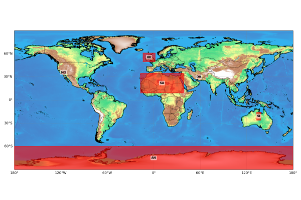
Notice that the geographic areas of the different regions vary considerably, as does the number of GCM grid locations contained within each region. Regional maxima and minima for Antarctic and Sahara in particular are taken over a large number of GCM locations in each case; inspection of Section SM7 provides context.

Location	Longitude interval	Latitude interval
Antarctic (AN)	(-180∘, -180∘)	(-90∘,-60∘)
Dasht-e Lut (DA)	(57∘,59.5∘)	(28∘,32∘)
Mojave (MO)	(-118.5∘,-114∘)	(34∘,37.25∘)
Sahara (SA)	(-17.1∘,38.5∘)	(9.3∘,34.6∘)
Simpson (SI)	(133∘,138∘)	(-26∘,-16∘)
UK (UK)	(-13.7∘,1.8∘)	(49.9∘,60.8∘)

Table 1: Summary of desert regions. List of geographic locations (and the UK as reference), with region acronyms in alphabetical order (column 1). Longitude-latitude bounding boxes per region (column 2).

For each combination of desert region, GCM and climate scenario, we examine output for up to five climate model ensemble members (denoted r* in the climate nomenclature; see Table 2 for examples) where available; these correspond to a common initialisation (i*), physics (p*) and forcing (f*) per GCM. For each combination of desert region, GCM, climate scenario and ensemble member, we therefore have access to time series, each consisting of 86 values, for annual maximum and annual minimum tas for the period 2015-210. The choice of GCM to analyse was entirely pragmatic: we accessed output from all GCMs available on the CEDA archive at the time of data harvesting.

GCM	Ensemble reference
ACCESS-CM2 (AC)	r1i1p1f1, r2i1p1f1, r3i1p1f1, r4i1p1f1, r5i1p1f1
CESM2 (CE)	r4i1p1f1, r10i1p1f1, r11i1p1f1
EC-Earth3 (EC)	r1i1p1f1, r4i1p1f1, r11i1p1f1
MRI-ESM2-0 (MR)	r1i1p1f1, r2i1p1f1, r3i1p1f1, r4i1p1f1, r5i1p1f1
UKESM1-0-LL (UK)	r1i1p1f2, r2i1p1f2, r3i1p1f2, r4i1p1f2, r8i1p1f2

Table 2: List of ensemble members considered per GCM. A total of five GCMs are used, listed in alphabetical order together with two-letter acronym (column 1). A total of up to five ensemble members is considered for each combination of climate variable and scenario (column 2), again depending on availability.

2.1 Compilation of spatio-temporal summaries for desert regions

We consider analysis of spatio-temporal block maxima and minima of tas, with temporal blocks corresponding to individual calendar years, and spatial blocks to each of the five desert regions (AN, DA, MO, SA and SI) and temperate UK control region. Henceforth, we refer to the spatio-temporal blocked data as “regional annual maxima” and “regional annual minima” for definiteness. For each combination of region, climate model, ensemble and scenario, regional annual maximum and minima data are extracted per calendar year from GCM output for the corresponding grid of locations (see Table 1). For illustration, Figure 2 shows spatial annual maxima and minima time series for the UK region from UKESM1-0-LL GCM. There is clear evidence for the effect of climate forcing, especially for maxima.

Figure 2: Regional annual maxima (left) and minima (right) time series of tas (K) for the UK “control” region from the UKESM1-0-LL GCM. Climate scenarios are distinguished by colour: SSP126 (green), SSP245 (orange), SSP585 (grey). Climate ensemble runs for each scenario, as listed in Table 2, are distinguished by line style.

Figure 3 shows regional annual maxima time series for all regions; corresponding regional annual minima time series are given in Figure SM1. For both regional annual maxima and minima, differences between “cold”, “temperate” and “hot” regions are clear, common to all GCMs. The extent of scenario effects varies somewhat by region and GCM for maxima in Figure 3, but less so for minima in Figure SM1.

2.2 Calibration

Outputs from GCMs are subject to bias. Therefore for interpretation, output of global climate models for variables such as tas are typically transformed to regional scale projections using downscaling procedures, and potentially further calibrated using observations. Here we work directly with GCM output to quantify the extent to which return values for tas change over the next century. We estimating the distribution of the difference between the 100-year return value for tas in 2025 and 2125 directly. This approach avoids introducing extra variability in our estimates related to uncertain downscaling and calibration models, at the expense of potential bias due to lack of calibration. As noted in [18], successful calibration requires that reasonable data are available for both model output and direct measurement, over a relatively large proportion of the time period of interest, (2015,2125) here. We cannot be confident that a calibration developed for the years (2015,2025) (for which measurements are available) is appropriate in 2125. Note also that the difference in 100-year return values for tas over the next century is unaffected by constant bias correction calibration.

Figure 3: Time series of regional annual maxima of tas (K) by GCM (rows: ACCESS-CM2, CESM2, EC-Earth3, MRI-ESM2-0 and UKESM1-0-LL) and region (column: : Antarctic, Dasht-e Lut, Mojave, Sahara, Simpson and UK). In each panel, climate scenarios are distinguished by colour: SSP126 (green), SSP245 (orange), SSP126 (grey). Climate ensemble runs for each scenario, as listed in Table 2, are distinguished by line style. Corresponding spatial annual minima time series are given in Figure SM1.

3 Methodology

We use parametric GEV regression to estimate models for regional annual maxima and minima of tas, for regions defined in Section 2.1. Generalising the approaches of [17] and [18], we assume that model parameters vary systematically over the period of observation as a function of time. Moreover, we constrain estimation across the three climate scenarios SSP126, SSP245 and SSP585 such that the estimated tail in the first year of GCM output (2015) is common to all scenarios. We consider GEV regressions with different complexities, discussed in Section 3.1. Model estimation is outlined in Section 3.2. The methods we consider for model selection are discussed in Section 3.3.

3.1 Model complexities

Indexing climate scenarios SSP126, SSP245 and SSP585 in terms of increasing forcing using variable $j$, $j=1,2,3$, we consider constant, linear and quadratic models for all of location $\mu$, scale $\sigma$ and shape $\xi$ of the GEV regression, of the form

$$\eta_{j}(t)=\eta_{0}+\tau\eta_{1j}+\tau^{2}\eta_{2j}$$ (1)

where $\eta\in\{\mu,\sigma,\xi\}$, for $i=1,2,...,P=86$, $j=1,2,3$, where $\tau=(i-1)/(P-1)$, and calendar year $t=i+2014$. Constant and linear parameterisations are imposed by setting $\eta_{1j}=\eta_{2j}=0$, and $\eta_{2j}=0$ respectively. For the location parameter $\mu$, we also consider an “asymptotic” parameterisation

$$\mu_{j}(t)=\mu_{0}^{a}+\mu^{a}_{1j}\left(\frac{1-\exp(-\tau/\mu^{a}_{2j})}{1-\exp(-1/\mu^{a}_{2j})}\right).$$ (2)

The asymptotic parameterisation for $\mu$ is considered since intuitively it might be expected that, under some circumstances at least, climate forcing might cause a shift of tas over time to a new stable level; it is reasonable to expect that this effect would be most identifiable for the location parameter. For the quadratic and asymptotic parameterisations, note that the values of $\eta_{j}(2015)=\eta_{0}$, $\eta\in\{\mu,\sigma,\xi\}$ and $\mu_{j}(2015)=\mu^{a}_{0}$, $j=1,2,3$ are common to all climate scenarios, imposing a common tail distribution for 2015. We also have $\eta_{j}(2100)=\sum_{k=1}^{3}\eta_{kj}$ for the quadratic parameterisation, and $\mu_{j}(2100)=\sum_{k=1}^{2}\mu^{a}_{kj}$. Note, for a given combination of GCM and region, different parametric forms are considered for each of $\mu$, $\sigma$ and $\xi$ as a function of time, but those forms are assumed common to all three climate scenarios.

We consider constant (C), linear (L), quadratic (Q) and asymptotic (A) parameterisations for GEV location $\mu$, and C, L and Q parameterisations for $\sigma$ and $\xi$. We refer to a specific model choice using an acronym indicating the parameterisations for $\mu$, $\sigma$ and $\xi$ in order. Thus, “QLC” indicates a GEV regression model with quadratic parameterisation for $\mu$, linear for $\sigma$ and constant for $\xi$. It is known that a sample is typically more informative for estimation of GEV location, then of scale then of shape (see e.g. discussion of [25]). For this reason, we can expect to identify more complex non-stationary behaviour in GEV location, then in scale, then in shape. As a result, we consider a total of 11 different GEV regression models, with the following complexities: CCC, LCC, QCC, ACC, LLC, LLL, QLC, QLL, QQC, QQL and QQQ.

3.2 Coupled non-stationary generalised extreme value regression

Asymptotic extreme value theory (e.g. [26], [27], [28]) shows that block maxima of random draws from a max-stable distribution follow the GEV distribution for sufficiently large block size. With the three climate scenarios again indexed by variable $j$, $j=1,2,3$, we assume access to a sample $D=\{x_{ij}\}_{i=1,j=1}^{P,3}$ of regional annual maxima $X_{j}(t)$ ($i=1,2,3,...,P;j=1,2,3;t=i+2014$) for analysis, for each combination of climate ensemble and region. Further we assume that for scenario $j$, the sample is drawn from a GEV distribution, with non-stationary location parameter $\mu_{j}(t)\in\mathbb{R}$, scale $\sigma_{j}(t)>0$, shape $\xi_{j}(t)\in\mathbb{R}$ and log density function

$$\log f_{j}(x) =\log f_{\text{GEVR}}(x|\mu_{j}(t),\sigma_{j}(t),\xi_{j}(t))$$

$$=\begin{cases}-\left[1+(\xi_{j}(t)/\sigma_{j}(t))\left(x-\mu_{j}(t)\right)\right]^{-1/\xi_{j}(t)}&\xi_{j}(t)\neq 0\\ \exp(-(x-\mu_{j}(t))/\sigma_{j}(t))&\xi_{j}(t)=0.\end{cases}$$ (3)

Model parameters $\eta_{j}\in\{\mu_{j},\sigma_{j},\xi_{j}\}$ vary with calender year $t$ as described in Equations 1 and 2, such that a common extreme value tail is fitted for the first year $t=2015$. The $T$-year return value $Q_{j}(t)$ for scenario $j$ in calendar year $t$ is estimated as the $p=1-1/T$ quantile of the corresponding GEV distribution function $F_{j}(x)$, so that

$$Q_{j}(t)=\begin{cases}(\sigma_{j}(t)/\xi_{j}(t))\left[\left(-\log p\right)^{-{\xi}_{j}(t)}-1\right]+{\mu}_{j}(t)&\xi_{j}(t)\neq 0\\ \mu_{j}(t)-\sigma_{j}(t)\log\left(-\log p\right)&\xi_{j}(t)=0.\end{cases}$$ (4)

Note that we only consider the case $T=100$ years in the current work for definiteness. Parameter estimation is performed using Bayesian inference as described in Section SM3, with

$$\ell(\boldsymbol{\theta})=\sum_{j=1}^{3}\sum_{i=1}^{P}\log f_{j}(x_{ij}|\boldsymbol{\theta})$$ (5)

as sample log likelihood, for parameter vector $\boldsymbol{\theta}=\{{\mu}_{0},{\sigma}_{0},{\xi}_{0},\{{\mu}_{1j},{\mu}_{2j},{\sigma}_{1j},{\sigma}_{2j},{\xi}_{1j},{\xi}_{2j}\}_{j=1}^{3}\}$ (for the full quadratic model QQQ, and the analogous sets for the other 10 GEV regression models). MCMC inference (see Section SM3) yields a sample $\{\boldsymbol{\theta}_{(s)}\}_{s=1}^{n_{S}}$ of joint posterior estimates from $f(\boldsymbol{\theta}|D)$ where $n_{S}=10,000$. These can be used to estimate the empirical distribution of quantities of interest, such as return values $Q_{j}(2025)$, $Q_{j}(2125)$, $j=1,2,3$, and the difference

$$\Delta Q_{j}=Q_{j}(2125)-Q_{j}(2025)$$ (6)

in return value over the 100 years from 2025 to 2125. Note that extreme value analysis for regional annual minima is performed via characterisation of the right hand tail of the distribution of negated data.

3.3 Model selection

We consider a large number of possible model parameterisations, and select between them using popular information criteria such as the Akaike information criterion (AIC), the Bayesian information criterion (BIC), the deviance information criterion (DIC) and the Wantanabe-Akaike Information Criterion (WAIC).

AIC ([7]) is an approximation to the Kullback-Leibler divergence between the fitted and underlying true model forms, and takes the form $\text{AIC}=\mathcal{D}(\hat{\boldsymbol{\theta}})+2p$, where $p$ is the number of parameters estimated, and $\mathcal{D}(\boldsymbol{\theta})$ is the sample deviance, defined by $\mathcal{D}(\boldsymbol{\theta})=-2\ell(\boldsymbol{\theta})=-2\log f(\boldsymbol{y}|\boldsymbol{\theta})$, evaluated at the maximum likelihood estimates $\hat{\boldsymbol{\theta}}$ of $\boldsymbol{\theta}$ maximising the sample log likelihood defined by Equation 5. Despite its name, BIC ([8]) is typically used in a frequentist setting, but has been used in conjunction with Bayesian inference (e.g. [29]). BIC is a large sample approximation to the Bayes factor, and defined by $\text{BIC}=\mathcal{D}(\hat{\boldsymbol{\theta}})+p\log n$ where $n$ is the number of observations for fitting. DIC ([9], [10]) is typically recommended for model selection in Bayesian inference, and like AIC and BIC, takes the form of “deviance estimate" plus “complexity penality”. The [9] and [10] definitions of DIC are given in Table 3, together with variants due to [30] and [31]. [3] recommend use of WAIC ([11]) to approximate out-of-sample predictive performance; WAIC again follows the same general form, as detailed in Table 3: WAIC is thought to be a more fully Bayesian approach for estimating out-of-sample expectation, starting with the computed log pointwise posterior predictive density and then adding a correction for effective number of parameters to adjust for over-fitting.

Abbreviation	Literature name	Lack of fit, A	Complexity penality, B	Reference
AIC1	AIC	$\mathcal{D}(\hat{\boldsymbol{\theta}})$	$2p$	[7]
AIC2	-	$\mathcal{D}(\mathbb{E}_{\boldsymbol{\theta}|D}[\boldsymbol{\theta}])$	$2p$	-
AIC3	Simplified BPIC	$\mathbb{E}_{\boldsymbol{\theta}|D}[\mathcal{D}(\boldsymbol{\theta})]$	$2p$	[31]
BIC1	BIC	$\mathcal{D}(\hat{\boldsymbol{\theta}})$	$p\log n$	[8]
BIC2	-	$\mathcal{D}(\mathbb{E}_{\boldsymbol{\theta}|D}[\boldsymbol{\theta}])$	$p\log n$	-
BIC3	-	$\mathbb{E}_{\boldsymbol{\theta}|D}[\mathcal{D}(\boldsymbol{\theta})]$	$p\log n$	-
DIC1	DIC	$\mathcal{D}(\mathbb{E}_{\boldsymbol{\theta}|D}[\boldsymbol{\theta}])$	$2p_{D1}$, Eqn 9	[9]
DIC2	DICalt	$\mathcal{D}(\mathbb{E}_{\boldsymbol{\theta}|D}[\boldsymbol{\theta}])$	$2p_{D2}$, Eqn 10	[10]
DIC3	Improved BPIC	$\mathbb{E}_{\boldsymbol{\theta}|D}[\mathcal{D}(\boldsymbol{\theta})]$	$2p_{D1}$, Eqn 9	[30], [31]
WAIC	WAIC	$-2$ lppd, Eqn 8	$2\ \sum_{i=1}^{n}\text{var}_{\boldsymbol{\theta}|D}\left[\log f(y_{i}|\boldsymbol{\theta})\right]$	[11]

Table 3: Information criteria (of the form $A+B$) explored for model selection. Sample size is $n$, the number of model parameters $p$. $\mathcal{D}=-2\log f(\boldsymbol{y}|\boldsymbol{\theta})$ is the sample deviance, or $-2$ times the sample log likelihood. $\hat{\boldsymbol{\theta}}$ is the maximum likelihood estimate for $\boldsymbol{\theta}$, and $\mathbb{E}_{\boldsymbol{\theta}|D}[\boldsymbol{\theta}]$ the posterior mean parameter estimate. $\mathbb{E}_{\boldsymbol{\theta}|D}[\mathcal{D}(\boldsymbol{\theta})]$ is the expected sample deviance under the posterior. Definitions of log pointwise predictive density lppd, and the complexity penalties $p_{D1}$ and $p_{D2}$ are given in the equations indicated, in the main text. BPIC refers to the Bayesian Predictive Information Criterion of [32], intended as an improved version of DIC.

Expectations and variances under the posterior distribution are evaluated using the MCMC sample, such that for function $g(\boldsymbol{\theta})$

$$\mathbb{E}_{\boldsymbol{\theta}|D}[g(\boldsymbol{\theta})]=\frac{1}{n_{S}}\sum_{s=1}^{n_{S}}g(\boldsymbol{\theta}_{(s)})\text{, and }\text{var}_{\boldsymbol{\theta}|D}[g(\boldsymbol{\theta})]=\frac{1}{n_{S}-1}\sum_{s=1}^{n_{S}}\left(g(\boldsymbol{\theta}_{(s)})-\mathbb{E}_{\boldsymbol{\theta}|D}[g(\boldsymbol{\theta})]\right)^{2}.$$ (7)

The log pointwise predictive density lppd is defined as

$$\text{lppd}=\sum_{i=1}^{n}\log\left(\frac{1}{n_{S}}\sum_{s=1}^{n_{S}}f(y_{i}|\boldsymbol{\theta}_{(s)})\right)$$ (8)

and the penalties $p_{D1}$ and $p_{D2}$ for DIC are defined as

$$p_{D1}=\mathbb{E}_{\boldsymbol{\theta}|D}[\mathcal{D}(\boldsymbol{\theta})]-\mathcal{D}(\mathbb{E}_{\boldsymbol{\theta}|D}[\boldsymbol{\theta}])$$ (9)

and

$$p_{D2}=2\ \text{var}_{\boldsymbol{\theta}|D}\left[\log f(\boldsymbol{y}|\boldsymbol{\theta})\right].$$ (10)

Inspired by the nature of the different combinations of “deviance” and “complexity penalty” terms associated with the different information criteria, we consider additional variants AIC2 and BIC2 of AIC and BIC utilising the posterior mean parameter estimate in place of the maximum likelihood estimate. In addition, variant BIC3 adapts BIC to use the posterior mean (predictive) deviance. Further, the analogous adaptation of AIC (to AIC3) results in the simplified BPIC introduced by Ando (and so could also be considered an extension of DIC). The original BPIC of [32] was developed to reduce over-fitting using DIC; a similar form of information criterion was previously proposed by [30]. The simplified BPIC of [31] is an approximation to BPIC, appropriate when the sample likelihood dominates the prior for well-specified candidate models. In comparing AIC, BIC and DIC, it might be suspected from Table 3 that the role of the complexity penalty is likely to be crucial, and that there is considerable similarity between some information criteria from nominally different classes.

Next, in Section 4, we evaluate the performance of all information criteria in a simulation study using data with known characteristics mimicking those of the regional annual maximum and minimum tas data. Subsequently, in Section 5, we adopt the best performing information criteria from the study, for model selection using the CMIP6 climate tas data.

4 Simulation study to examine the predictive performance of different model selection criteria

As discussed in Section 3.3, there is no reason to expect that different model selection criteria will choose the same models complexities (defined in Section 3) for scenario-coupled GEV regression for a given application. For example, as can be seen from Table 3, BIC penalises model complexity relatively severely, and might therefore be expected to produce more parsimonious models, possibly advantageous in the context of extreme value modelling.

Figure 4: Simulation study design. Variation of GEV location ($\mu$; top), scale ($\sigma$; middle) and shape ($\xi$; bottom) in time for three scenarios (red, green and blue), for each of 11 data-generating processes (CCC to QQQ; columns left to right).

We perform a simulation study using the 11 data generating processes visualised in Figure 4, one for each of the 11 model complexities listed in Section 3.1. The figure shows variation of GEV location, scale and shape parameters for three “scenarios” shown in red, green and blue; these choices of parameter variation were informed by inspection and initial analysis of the CMIP6 regional annual maximum and minimum data. We do not claim that the 11 examples used are representative of all possible non-stationary GEV processes, but they do reasonably reflect the characteristics of the CMIP6 data. We generate $n_{R}=100$ sample realisations $D_{k}$, $k=1,2,...,100$ from each of the 11 processes, each sample consisting of 86 “yearly” observations for each of three scenarios. We then fit all 11 model forms, ranging from CCC (i.e. constant GEV location, scale and shape) to QQQ (i.e. quadratic variation of GEV location, scale and shape in time) to each sample using MCMC, obtaining a chain of parameter estimates from the joint posterior distribution $f(\boldsymbol{\theta}|D)$ (see Section 3.2). Then, for each combination of data-generating process and fitted model, we evaluate the root mean square error

$$\text{RMSE}=(\frac{1}{3n_{R}n_{S}}\sum_{j=1}^{3}\sum_{k=1}^{n_{R}}\sum_{s=1}^{n_{S}}(\Delta Q_{j}^{*}-\Delta Q_{j(s)}|D_{k}])^{2})^{1/2}$$ (11)

in estimation of the difference $\Delta Q_{j}$ in return values over scenarios, $j=1,2,3$, where $\Delta Q_{j}^{*}$ is the true value, and $\Delta Q_{j(s)}|D_{k}$ is posterior estimate of $\Delta Q_{j}$ corresponding to iteration $s$, $s=1,2,...,n_{S}$ from the MCMC chain for data realisation $D_{k}$, $k=1,2,...,n_{R}$.

Finally, we use each of the model selection information criteria in Table 3 to choose optimal model complexities, and corresponding estimates for RMSE; these are shown in Figure 5, as a function of data-generating process and model selection information criterion.

Figure 5: RMSE estimates (see Equation 11) from the simulation study, for different combinations of data-generating process (CCC to QQQ; x-axis) and model selection information criterion (AIC1 to WAIC; coloured lines). Note that for data-generating process CCC, all of BIC1, BIC2 and BIC3 always select the correct CCC model form, resulting in RMSE=0 (not shown on the $\log_{10}$-scale y-axis.)

From the figure, it is obvious that variants of AIC and BIC perform considerably better than DIC variants and WAIC, and that BIC performs somewhat better than AIC. Moreover, there is little difference between the “within-class” performance of variants of AIC, of BIC, or of DIC. In hindsight, the poor performance of DIC and WAIC is probably to be expected (see e.g. the discussion of Section 7.3 of [4], and Section SM1.1). Given these results, we adopt one variant of BIC (BIC3) and one of AIC (AIC3) for model selection applied to the CMIP6 data in Section 5, noting that we could have adopted any of the BIC and AIC variants without loss of generality.

5 Results

In this section, we apply the GEV regression methodology from Section 3 and optimal model selection criteria BIC3 and AIC3 from Section 4 to estimate changes in 100-year return values over the period (2025,2125) for samples of regional annual maxima and minima of tas, for different choices of desert region, GCM and climate ensemble. Results for regional annual maxima are summarised in Section 5.1 and Section SM4, and for regional annual minima in Section 5.2 and Section SM5.

5.1 Regional annual maxima

A typical result for GEV regression for regional annual maxima, for a specific choice of region and GCM and all climate ensembles, is visualised in Figure 6 (for the Sahara region using the UKESM1-0-LL GCM). Results for all 30 combinations of region and GCM are summarised using the same template in Figures SM2-SM31. The top left panel shows variation of values of information criteria (BIC3 and AIC3; different line styles) for fitting of models of different complexity (CCC to QQQ; x-axis), using data for each of the available climate ensembles (line colours). The optimal model selected is indicated by a red circle (BIC3) and blue cross (AIC3). The other three panels summarise the posterior distribution of the difference $\Delta Q_{j}$, $j=1,2,3$ in 100-year return value over the period (2025,2125) (see Equation 6) as a function of fitted model and climate ensemble, under climate scenarios SSP126 ($j=1$, top right), SSP245 ($j=2$, bottom left) and SSP585 ($j=3$, bottom right).

Figure 6: Summary of scenario-coupled GEV regression for regional annual maxima of the Sahara region using UKESM1-0-LL GCM data. Top left: plots of BIC3 (solid line) and AIC3 (dashed line) for each available ensemble (distinguished by colour, see Table 2 and legend in bottom-right panel); optimal model choice using BIC3 (AIC3) indicated using red disc (blue cross). Top right: box-whisker plots summarising the distribution of the difference in the 100-year return value between 2025 and 2125 ($\Delta Q_{1}$; see Equation 6) for climate scenario SSP126 as a function of fitted model complexity (x-axis) and ensemble (distinguished by colour, with consistent ensemble colouring across panels); location of horizontal centre line of each box indicates posterior median of $\Delta Q_{1}$; location of top (bottom) side of each box indicates 75%ile (25%ile) point, and top (bottom) of whiskers the 97.5%ile (2.5%ile) point of the posterior distribution. Bottom left and right: analogues of top right for scenarios SSP245 ($\Delta Q_{2}$) and SSP585 ($\Delta Q_{3}$). Value of $\Delta Q_{j}$, $j=1,2,3$ under model CCC is identically zero, and is omitted from bottom panels when convenient to provide better illustration of the variation in estimates under more complex models.

For the Sahara region using the UKESM1-0-LL GCM, the top left panel indicates that BIC3 prefers QCC models, with quadratic variation of GEV location in time, but stationary GEV scale and shape. AIC3 tends to prefer somewhat more complex models. The remaining panels show that the uncertainty in $\Delta Q$ increases with fitted model complexity, as does between-ensemble variability. For the BIC3-optimal QCC model fits, there is general agreement across climate ensembles: approximately no change in $\Delta Q$ under scenario SSP126, but changes of around 3K and 11K under SSP245 and SSP585. Clearly, the choice of fitted model has a large effect on our estimate of $\Delta Q$. The general features of results for other combinations of region and GCM (in Figures SM2-SM31) are similar: BIC3 tends to select more parsimonious models, with LCC the most frequent choice (see Section 6.1).

Figure 7 summarises inferences for $\Delta Q_{j}$, $j=1,2,3$ of regional annual maxima using the BIC3-optimal GEV regression models, aggregated over climate ensembles, as a function of region and GCM. Aggregation is achieve by simply combining the samples of posterior estimates for $\Delta Q$ corresponding to different ensembles into one aggregate sample. The figure indicates general agreement across GCM and region, with somewhat larger increases in $\Delta Q$ in Dasht-e Lut, Sahara and Simpson, and lowest in the Antarctic. The UK control region does not look unusual alongside the “hot” desert regions. Corresponding estimates per climate ensemble are given in Figure SM32, showing good general agreement across ensembles. The corresponding summaries for AIC3-optimal models is shown in Figures SM33-SM34.

Figure 7: Summary of inferences for return value differences $\Delta Q_{j}$, $j=1,2,3$ (see Equation 6) of regional annual maxima using BIC3 for model selection, aggregated over climate ensemble. Each panel shows box-whisker plots summarising the posterior distribution of $\Delta Q$ for climate scenarios SSP126 ($j=1$, green), SSP245 ($j=2$, orange) and SSP585 ($j=3$, grey) and each of five GCMs (ACCESS-CM2, CESM2, EC-Earth3, MRI-ESM2-0, UKESM1-0-LL). Left to right, top to bottom, panels show inferences for the Antarctic, Dasht-e Lut, Mojave, Sahara, Simpson and UK regions.

An overall summary for regional annual maxima is presented in Figure 8, where the estimated posterior distribution of $\Delta Q_{j}$, $j=1,2,3$ using BIC3 for model selection is aggregated over both climate ensemble and GCM. The corresponding summary for AIC3 model selection is given in Figure SM35.

Figure 8: Summary of inferences for return value differences $\Delta Q_{j}$, $j=1,2,3$ (see Equation 7) of regional annual maxima using BIC3 for model selection, aggregated over climate ensemble and GCM. Box-whisker plots summarise the posterior distribution of $\Delta Q$ for climate scenarios SSP126 ($j=1$, green), SSP245 ($j=2$, orange) and SSP585 ($j=3$, grey) for the Antarctic, Dasht-e Lut, Mojave, Sahara, Simpson and UK regions.

It is noteworthy that the 95% credible intervals for $\Delta Q$ under scenario SSP126 include zero (i.e. no change), whereas they do not under SSP245 and SSP585, suggesting significant increases in the 100-year return value for tas over the next 100 years under the latter scenarios.

5.2 Regional annual minima

Inferences for regional annual minima are presented using the same template used for maxima. Results for all 30 combinations of region and GCM are summarised Figures SM36-SM65. The general characteristics of the figures are similar to those for regional annual maxima. The 100-year return value for tas typically increases in time, but sometimes there is no obvious trend. The extent of any change observed is less marked. For example, for the Sahara and UKESM1-0-LL GCM in Figure SM55, BIC3 chooses LCC (rather than QCC), with typical changes of 2K, 4K and 7K under SSP126, SSP245 and SSP585. These differences reflect those visible in Figure 2.

Figure 9 summarises inferences for $\Delta Q_{j}$, $j=1,2,3$ of regional annual minima using the BIC3-optimal GEV regression models, aggregated over climate ensembles, as a function of region and GCM; estimates per climate ensemble are given in Figure SM66. The corresponding summaries for AIC3-optimal models is shown in Figures SM67-SM68.

Figure 9: Summary of inferences for return value differences $\Delta Q_{j}$, $j=1,2,3$ (see Equation 6) of regional annual minima using BIC3 for model selection, aggregated over climate ensemble. For details, see Figure 7.

There is in general reasonable between-ensemble agreement (e.g. Figure SM66), but poorer agreement between GCMs; for example, MRI-ESM2-0 yields CCC models for Dasht-e Lut, resulting in $\Delta Q=0$ under all scenarios. Results for the Antarctic are similar to those for “hot” regions. The overall summary for regional annual minima in Figure 10 gives estimates for the posterior distribution of $\Delta Q$ using BIC3 for model selection aggregated over both climate ensemble and GCM. It can be seen that many of the 95% credible intervals include zero, even under SSP245 and SSP585 scenarios, indicating less confidence in the increasing trend observed. The corresponding summary for AIC3 model selection is given in Figure SM69.

Figure 10: Summary of inferences for return value differences $\Delta Q_{j}$, $j=1,2,3$ (see Equation 7) of regional annual minima using BIC3 for model selection, aggregated over climate ensemble and GCM. For details, see Figure 8.

6 Discussion and conclusions

This paper presents is a pragmatic approach to model selection in Bayesian extreme value regression. We use the approach to estimate the change in the value of the 100-year return value $\Delta Q$ for near-surface atmospheric temperature tas over the period (2025,2125), and its variability from CMIP6 model output for desert regions. Model fitting is performed using non-stationary generalised extreme value (GEV) regression and Bayesian inference. The GEV parameters $\mu,\sigma,\xi$ are assumed to exhibit parametric variation with time. Models for $\mu,\sigma,\xi$ in time with different complexities are considered and their performance quantified and compared using variants of the Bayesian and Akaike information criteria. These specific choices of criteria were found to be optimal in terms of minimising the root mean square error of predictions of $\Delta Q$ in a simulation study. We believe the work provides a number of interesting statistical and physical insights.

6.1 Distribution of complexity of fitted models

Numerous model selections are performed in the current analysis. The complexity of optimal model selections over all combinations of region, maximum or minimum, GCM and climate ensemble provides a general indication of the information content of the time series data. For example, the histograms in Figure 11 indicate the frequency with which each of the 11 candidate model complexities is chosen, in application to regional annual maxima (left hand side) and minima, over all combinations of region, GCM and climate ensemble, using BIC3 for model selection.

Regional annual maxima

Regional annual minima

Figure 11: Complexities of optimal fitted models for regional annual maxima (left) and minima (right) using BIC3 for model selection.

Comparison of the left and right hand sides of the figure show that more complex models can be justified for regional annual maxima. However, in general, selected models tend to incorporate non-stationarity in the GEV location parameter $\mu$ only, and very rarely in GEV scale $\sigma$ and shape $\xi$. For regional annual maxima, models QCC and ACC together account for almost half the selected model forms. For comparison, Figure SM75 shows the corresponding histograms for model selection using AIC3. Relative to BIC3, model selection using AIC3 results in more complex model forms; regardless, models stationary with respect to $\sigma$ and $\xi$ are more prevalent.

6.2 An initial comparison with Bayesian model averaging

The current work has focussed on model selection from a set of 11 candidate models CCC to QQQ with different complexities. An alternative approach, avoiding selection of a single optimal model complexity for prediction of $\Delta Q$, it to estimate a weighted sum of all candidates which has good predictive performance for $\Delta Q$. Here, we provide an initial comparison of our model selection procedure with Bayesian model averaging (BMA).

In BMA, we take a linear combination of posterior predictive densities for $\Delta Q$ from each of $n_{M}=11$ candidate models $\{$CCC, LCC, …, QQQ$\}$ $=\{M_{1},M_{2},...,M_{11}\}$ in order for convenience. Specifically, for the 3-vector $q=[\Delta Q_{1},\Delta Q_{2},\Delta Q_{3}]$, we estimate the average predictive posterior density for $q$ as

$$f_{S}(q|D)=\sum_{m=1}^{n_{M}}w_{m}f(q|M_{m},D)$$ (12)

where $f(q|M_{m},D)$ is the posterior predictive density for $q$ estimated from data $D$ using model $M_{m}$, $m=1,2,...,n_{M}$. We estimate the set of weights $\{w_{m}\}$ using the stacking procedure of [16] outlined in Section SM9.

We compare the performance of Bayesian model averaging to model selection using BIC3, in application to the estimation of $\Delta Q_{j}$, $j=1,2,3$ using the simulation study data from Section 4, and the CMIP6 climate data for the Sahara region and UKESM1-0-LL GCM.

		Data-generating model ($n_{R}=100$ realisations)												CMIP6 data
		CCC	LCC	QCC	ACC	LLC	LLL	QLC	QLL	QQC	QQL	QQQ	LCC	SA-UK
		Proportions of fitted models selected using BIC3											BMA weights $w_{m}$, $m=1,2,...,11$
Fitted model	CCC	1.00	0.68	0.10	0.18	0.05							0.14 (0.00,0.59)	0.00
	LCC		0.31	0.90	0.78	0.01		0.02					0.40 (0.00,1.00)	0.00
	QCC				0.03								0.00 (0.00,0.79)	0.21
	ACC				0.02								0.18 (0.00,0.91)	0.42
	LLC		0.01			0.94	0.93	0.98	0.97	0.99	0.84	0.94	0.07 (0.00,0.74)	0.00
	LLL						0.07		0.03		0.13	0.06	0.04 (0.00,0.46)	0.00
	QLC									0.01	0.03		0.01 (0.00,0.21)	0.25
	QLL												0.01 (0.00,0.00)	0.09
	QQC												0.01 (0.00,0.12)	0.00
	QQL												0.01 (0.00,0.12)	0.00
	QQQ												0.03 (0.00,0.36)	0.02
	RMSE	0.00	3.06	2.82	2.73	4.38	9.30	3.86	10.1	7.38	17.3	17.3	3.98	-

Table 4: Assessment of fitted models: (a) Columns 3-13 give the proportions of optimal selected models (from the 11 candidates CCC to QQQ; rows) using the BIC3 information criterion, corresponding to each of $n_{R}=100$ sample realisations from data-generating models with different complexities (CCC to QQQ; columns); (b) Column 14 gives the correspond average BMA weights per fitted model, again estimated using $n_{R}=100$ sample realisations, with marginal 95% uncertainty bands; (c) Column 15 gives BMA weights, averaged over climate ensembles, for the CMIP6 sample data of regional annual maxima for the Sahara from the UKESM1-0-LL GCM. Values are rounded to two decimal places, and zero values of proportions are not shown to aid interpretation. (Note the curious BMA weight estimate for model QLL, arising because values for all but one realisation are zero to two decimal places.)

Table 4 summarises the distribution of selected model complexities in BIC3-based model selection for different data-generating models. Specifically, the same $n_{R}=100$ realisations of each of the $11$ data-generating models CCC to QQQ, reported in the simulation study of Section 4, were re-used. Each of the $n_{M}$ candidate models CCC to QQQ is fitted in turn, and BIC3 used to select the optimal fitted model. Columns 3-13 of the table report the proportion of fitted models of different complexities, for each complexity of data-generating model: thus, for an LLL data-generating model, the LLC fitted model was selected by BIC3 for 93 of the 100 sample realisations, and LLL for the remaining 7 realisations. It can be seen that realisations of stationary samples (CCC) always result in selection of stationary (CCC) fitted models. When sample realisations include non-stationary variation (i.e. either linear, L or quadratic, Q) of GEV location $\mu$ or scale $\sigma$, this typically results in the selection of a fitted model with linear variation (L) in the corresponding parameter. Fitted models incorporating variation in GEV shape $\xi$ are rarely selected, regardless of the data-generating process. Hence, the optimal fitted model complexity corresponding to all the data-generating models LLL to QQQ is LLC. The fact that fitted models with quadratic (Q) variation in $\mu$ and $\sigma$, and any non-stationary (i.e. L or Q) with respect to $\xi$, tend not to be fitted, is attributed to the small sample sizes (86 years $\times$ three scenarios) in the current work. It is interesting that the typical literature presumption for parametric GEV regression applied to annual maxima of tas in time is linear variation in $\mu$ and $\sigma$, and stationary $\xi$. We would expect, were larger samples used, that more complex selected models would occur.

The table also gives optimal BMA weights $w_{m}$, $m=1,2,...,n_{M}$ estimated from the stacking procedure (Equation 12, [16] and Section SM9) from $n_{R}=100$ realisations of the LCC data-generating model only. The penultimate column of the table gives the average weight (over realisations) attributed to each fitted model complexity, together with empirical marginal 95% uncertainty bands for each weight. It is intuitively reassuring that the largest weights correspond to the LCC and ACC fits. The estimated RMSE over the $n_{R}$ sample realisations for BIC3-selected models is 3.06, calculated using Equation 11; the corresponding estimate for Bayesian model averaging is 3,98, calculated using Equation SM8. That the BIC model selection procedure outperforms the model average is perhaps not surprising here, because the choice of model selection criterion was made specifically to minimise RMSE is estimation of $\Delta Q$. Finally, the table gives BMA weights (averaged over the 5 climate ensembles) for the CMIP6 data corresponding to annual maxima from the Sahara region and the UKESM1-0-LL GCM, noting from Figure 6 that BIC3 selects the QCC model for these data. The largest weights are seen to correspond to the ACC, QLC and QCC models. It appears from these preliminary results that the stacking BMA approach favours somewhat more complex models than BIC3, perhaps more like AIC3, resulting in poorer performance in estimating $\Delta Q$. The authors plan a further study to examine the performance the stacking BMA method thoroughly.

6.3 Are extreme regional annual maxima increasing in size more quickly?

Figure 12: Summary of inferences for the difference $\Delta\Delta Q_{j}$, $j=1,2,3$ (see Eqution 13) between $\Delta Q$ values of regional annual maxima and minima. BIC3 was used for model selection, and posterior distributions aggregated over climate ensemble and GCM. For other details, see Figure 8.

The distributions of $\Delta Q_{j}$, $j=1,2,3$ (see Equation 6) for regional annual maxima and minima are given in Figures 8 and 10 respectively. It is apparent that there is in general an upward trend for both maxima and minima across desert and UK control regions, but that the extent of increase of regional annual maxima is in general greater. To quantify this, Figure 12 shows the differences $\Delta\Delta Q_{j}$, $j=1,2,3$ for each combination of climate scenario and region, aggregated over climate ensemble and GCM.

$$\Delta\Delta Q_{j}=\Delta Q_{j}^{\text{max}}-\Delta Q_{j}^{\text{min}}$$ (13)

where $\Delta Q_{j}^{\text{max}}$ and $\Delta Q_{j}^{\text{min}}$ refer to $\Delta Q_{j}$ for regional annual maxima and minima respectively, $j=1,2,3$. 95% credible intervals in Figure 12 include zero in every case, suggesting that there are no strong trends in $\Delta\Delta Q$. Nevertheless, it is interesting, for all regions except for Antarctic, that there is a mild increasing trend in median $\Delta\Delta Q$ with increased forcing, suggesting that extreme quantiles of regional annual maxima are increasing (i.e. warming) at a greater rate than those of minima, and that this difference increases with climate forcing. The Antarctic shows the opposite trend: under scenario SSP585 in particular, the value of median $\Delta\Delta Q_{3}$ is around -3K: extremes of regional annual minima of tas are warming faster than those of regional annual maxima. The corresponding result for AIC3 model selection is given in Figure SM70.

6.4 Conclusions

When competing models of different complexity are considered in non-stationary extreme value modelling using small samples, care must be taken in model selection. The relative performance of different “information criteria” (including AIC, BIC, DIC and WAIC) for model selection with respect to a specific prediction task cannot be easily anticipated. We recommend that a simulation study is undertaken, using relevant data, to identify which information criteria perform best for the prediction task. For the current work, focussing on predicting the difference $\Delta Q$ in the 100-year return value over the period (2015,2125), of regional annual maxima and minima of tas using Bayesian inference, we find that the Bayesian information criterion (BIC) provides optimal predictive performance. We also demonstrate that Bayesian model averaging provides a feasible alternative to model selection, but - using the stacking approach considered here - at considerably increased computational cost.

Using optimal model selection, for regional annual maxima and minima of tas in desert regions (and UK “control” region), there is general consistency across inferences for $\Delta Q$ from different climate scenarios, for a given combination of region and GCM. There is further general consistency across GCMs for a given region. The general pattern is of $\Delta Q$ increasing with climate forcing, and that higher increases are seen in the Dasht-e Lut, Sahara, Simpson and UK regions under the SSP585 scenario. Using inferences aggregated over GCM and climate ensemble, there is evidence for significant increases in $\Delta Q$ for regional annual maxima under scenarios SSP245 and SSP585 for all desert regions. Trends for regional annual minima are generally similar, but evidence is weaker. For the Antarctic region, the estimated median difference between $\Delta Q$ for annual maxima and minima decreases with increasing forcing, suggesting that 100-year return values of annual minima are increasing more quickly than those for annual maxima.

Resources

Comprehensive supplementary material accompanying this research can be found at https://ygraigarw.github.io/LchEA26_CoupledGEVR.pdf. Data and software are provided at https://github.com/Callum-Leach/SCCER.

References

- \bibcommenthead
- Zanini et al. [2020] Zanini, E., Eastoe, E., Jones, M.J., Randell, D., Jonathan, P.: Flexible covariate representations for extremes. Environmetrics 31, 2624 (2020)
- Vehtari and Ojanen [2012] Vehtari, A., Ojanen, J.: A survey of Bayesian predictive methods for model assessment, selection and comparison. Statist. Surv. 6, 142–228 (2012)
- Gelman et al. [2013] Gelman, A., Carlin, J.B., Stern, H.S., Dunson, D.B., Vehtari, A., Rubin, D.B.: Bayesian Data Analysis. Chapman and Hall/CRC, Boca Raton, FL (2013)
- Gelman et al. [2014] Gelman, A., Hwang, J., Vehtari, A.: Understanding predictive information criteria for Bayesian models. Stat. Comput. 24, 997–1016 (2014)
- Kim et al. [2017] Kim, J., Sun, Y., Kim, J.-S., Kang, S., Lee, J.-H.: Appropriate model selection methods for nonstationary generalized extreme value models. J. Hydrol. 549, 538–550 (2017)
- Zhang et al. [2023] Zhang, J., Yang, Y., Ding, J.: Information criteria for model selection. Wiley Interdiscip. Rev. Comput. Stat. 15, 1607 (2023)
- Akaike [1974] Akaike, H.: A new look at the statistical model identification. IEEE Trans. Autom. Control 19, 716–723 (1974)
- Schwarz [1978] Schwarz, G.: Estimating the dimension of a model. Ann. Stat. 6, 461–464 (1978)
- Spiegelhalter et al. [2002] Spiegelhalter, D.J., Best, N.G., Carlin, B.P., Linde, A.: Bayesian measures of model complexity and fit. J. Roy. Statist. Soc. B 64, 583–639 (2002)
- Gelman et al. [2004] Gelman, A., Carlin, J.B., Stern, H.S., Rubin, D.B.: Bayesian Data Analysis. Chapman and Hall/CRC, Boca Raton, FL (2004)
- Watanabe [2013] Watanabe, S.: A widely applicable Bayesian information criterion. J. Mach. Learn. Res. 14, 867–897 (2013)
- Vehtari et al. [2017] Vehtari, A., Gelman, A., Gabry, J.: Practical Bayesian model evaluation using leave-one-out cross-validation and WAIC. Statistics and Computing 27, 1413–1432 (2017)
- Warner [2004] Warner, T.T.: Desert Meteorology. Cambridge University Press, Cambridge, UK (2004)
- Steel [2019] Steel, M.F.J.: Model averaging and its use in economics. arXiv preprint (2019) arXiv:1709.08221v3 [stat.ME]
- Wasserman [2000] Wasserman, L.: Bayesian model selection and model averaging. J. Math. Psychol. 44, 92–107 (2000)
- Yao et al. [2018] Yao, Y., Vehtari, A., Simpson, D., Gelman, A.: Using stacking to average Bayesian predictive distributions (with discussion). Bayesian Anal. 13, 917–1007 (2018)
- Ewans and Jonathan [2023] Ewans, K., Jonathan, P.: Uncertainties in estimating the effect of climate change on 100-year return period significant wave heights. Ocean Eng. 272, 113840–117 (2023)
- Leach et al. [2025] Leach, C., Ewans, K., Jonathan, P.: Changes over time in the 100-year return value of climate model variables. Ocean Eng. 324, 120605 (2025)
- Kharin and Zwiers [2005] Kharin, V.V., Zwiers, F.W.: Estimating extremes in transient climate change simulations. J. Clim. 18, 1156–1173 (2005)
- Zwiers et al. [2011] Zwiers, F.W., Zhang, X., Feng, Y.: Anthropogenic influence on long return period daily temperature extremes at regional scales. J. Clim. 24, 881–892 (2011)
- Kharin et al. [2013] Kharin, V.V., Zwiers, F.W., Zhang, X., Wehner, M.: Changes in temperature and precipitation extremes in the CMIP5 ensemble. Climatic Change 119, 345–357 (2013)
- Kharin et al. [2018a] Kharin, V.V., Flato, G.M., Zhang, X., Gillett, N.P., Zwiers, F., Anderson, K.J.: Risks from climate extremes change differently from 1.5∘C to 2.0∘C depending on rarity. Earth’s Future 6, 704–715 (2018)
- Kharin et al. [2018b] Kharin, V.V., Zwiers, F.W., Zhang, X., Wehner, M.: Risks of precipitation and temperature extremes in CMIP6 models. Earth’s Future 6, 630–650 (2018)
- Leach and Jonathan [2026] Leach, C., Jonathan, P.: Scenario-coupled climate extreme-value regression (SCCER). GitHub https://github.com/Callum-Leach/SCCER (2026)
- Jonathan et al. [2008] Jonathan, P., Ewans, K.C., Forristall, G.Z.: Statistical estimation of extreme ocean environments: The requirement for modelling directionality and other covariate effects. Ocean Eng. 35, 1211–1225 (2008)
- Coles [2001] Coles, S.: An Introduction to Statistical Modelling of Extreme Values. Springer, Berlin (2001)
- Beirlant et al. [2004] Beirlant, J., Goegebeur, Y., Segers, J., Teugels, J.: Statistics of Extremes: Theory and Applications. Wiley, Chichester, UK (2004)
- Jonathan and Ewans [2013] Jonathan, P., Ewans, K.: Statistical modelling of extreme ocean environments with implications for marine design : a review. Ocean Eng. 62, 91–109 (2013)
- Neath and Cavanaugh [2012] Neath, A.A., Cavanaugh, J.E.: The Bayesian information criterion: background, derivation, and applications. Wiley Interdiscip. Rev. Comput. Stat. 4, 199–203 (2012)
- van der Linde [2005] Linde, A.: DIC in variable selection. Stat. Neerl. 59, 45–56 (2005)
- Ando [2011] Ando, T.: Predictive Bayesian model selection. Am. J. Math. Manag. Sci. 31, 13–38 (2011)
- Ando [2007] Ando, T.: Bayesian predictive information criterion for the evaluation of hierarchical Bayesian and empirical Bayes models. Biometrika 94, 443–458 (2007)