The Bragg Frequency Convertor: A Meeting Between Spatial and Temporal Periodicities For Selective Parametric Frequency Translation

Abstract

This study introduces the Bragg Frequency Convertor, a spatial-temporal-periodic grating that extends the concept of conventional Bragg gratings into the dynamic domain to achieve pure parametric frequency conversion. By time-modulating either the high-index or low-index layers of a quarter-wave Bragg grating, we demonstrate selective and directional frequency conversion: Modulation of the high-index layers selectively yields down-conversion, whereas modulation of the low-index layers leads to up-conversion. Such a pure frequency conversion emerges from the synergistic interplay of spatial and temporal periodicities. The output is thus dominated by the converted frequency, with the carrier and undesired time harmonics suppressed. We derive a coupled-mode theory explaining such a layer-dependent phase matching and validate it with full-wave simulations, showing tunable conversion efficiency via modulation phase. The advance presented here lies in recognizing the conventional Bragg grating not as a passive partner but as an enabling scaffold: its intrinsic spatial periodicity is exploited to impose the precise spectral constraints required for efficient temporal modulation and the generation of pure parametrically converted signals. This work establishes temporal Bragg gratings as a versatile platform for reconfigurable and spurious-free frequency conversion, with applications in optical systems, signal processing, spectral engineering, and quantum photonics.

I Introduction

The pursuit of dynamic control over light-matter interaction has driven optics and photonics research beyond static structures and into the domain of dynamic media [1, 2, 3, 4, 5, 6, 7, 6, 8, 9, 10]. By judiciously modulating the electromagnetic properties of a material in time, it is possible to break Lorentz reciprocity, create non-reciprocal devices, and realize optical isolation without magnetic materials [11, 12, 13]. More profoundly, temporal modulation can act as a synthetic pump that injects energy into an optical system, enabling parametric processes such as nonreciprocal transmission and isolation [14, 15, 16, 17, 18, 19], spatiotemporal diffraction [20], amplification [21, 22, 23, 24, 25, 26], frequency conversion [27, 28, 29, 30, 31, 32], beamsplitting [23], absorption [33, 4], multifunctionality [34], and wave mixing and frequency multiplexing [35, 36, 37, 38, 39]. Among these parametric phenomena, pure frequency conversion [28, 29], the coherent translation of an optical signal from one frequency to another with minimal residual power at the original frequency, stands as a cornerstone for applications in classical and quantum communications, spectral imaging, and frequency-domain signal processing.

Conventional approaches to frequency conversion rely on nonlinear optical crystals or waveguides, where a strong pump beam mediates energy transfer between signal and idler waves via second- or third-order nonlinearities. While effective, these methods often require stringent conditions, high pump powers, and bulk materials, limiting their integration into compact photonic circuits. However, achieving pure conversion, where the output is dominated by the target frequency with strong suppression of the original carrier, remains challenging in simple modulated waveguides, as the input frequency typically co-propagates and transmits alongside the generated sidebands. In parallel, spatially periodic structures, photonic crystals and Bragg gratings, have long been used to engineer the density of optical states and control the propagation of light [40, 41]. A Bragg grating, in its simplest form, is a stack of alternating high- and low-index layers designed to create a photonic stopband: a range of frequencies over which light is strongly reflected [42, 43, 44, 45, 46, 47, 48, 49, 50]. However, a critical question remains: can we achieve pure frequency conversion, where the output is dominated by the shifted frequency with the original carrier suppressed, in a compact, integrated platform?

In this work, we answer this question affirmatively by introducing the Bragg Frequency Convertor, a spatial-temporal-periodic grating where pure parametric frequency conversion emerges from the synergistic interplay of spatial and temporal periodicities yielding distributed periodic spatiotemporal scattering. Within each time-modulated layer, the oscillating refractive index continuously generates waves at high-order time harmonics. These temporal reflections and transmissions originate throughout the volume of each modulated layer, propagating in both forward and backward directions. They are not confined to interfaces, as in conventional spatial scattering, but are distributed sources that fill the structure. Each modulation period produces a new set of these wavelets, creating an array of periodic temporal reflections and transmissions. These temporally generated wavelets then propagate through the periodic stack, encountering the spatial interfaces that produce spatial reflections. The key to pure conversion lies in the coherent summation of all these contributions. The favored sideband lies outside the Bragg stopband and propagates freely, with wavelets from different layers and different time periods adding constructively when the accumulated propagation phase matches the modulation periodicity. The unfavored sideband lies inside the stopband and remains trapped. The carrier itself is strongly reflected by the spatial periodicity and cannot transmit.

The result is a transmitted output spectrum dominated by a single, pure converted frequency, with the original carrier reflected. Here, the temporal Bragg grating is established as a versatile platform for on-demand frequency synthesis. By merging the spatial periodicity of a Bragg filter with the parametric power of temporal modulation, we create a device where the direction of frequency conversion (up or down) is determined by a simple design choice, which layer to modulate, and the conversion efficiency is controlled electronically via the modulation phase. We present a comprehensive coupled-mode theory that explains the layer-selective phase-matching condition, validate it with rigorous numerical simulations, and outline the design principles for optimal conversion. This Bragg Frequency Converter offers a new pathway toward integrated, low-power, and reconfigurable frequency-shifting devices for future classical and quantum photonic systems.

Figure 1: Schematic of the Bragg Frequency Convertor. (a) Up-conversion configuration: low-index layers are time-modulated. The device consists of $N$ periods of alternating high-index and low-index layers, each satisfying the quarter-wave condition at the design frequency. The low-index layers are modulated targeting up-conversion to $f_{+1}=f_{0}+f_{m}$, while the high-index layers remain static. An incident wave at $f_{0}$ enters from the left. The static Bragg grating formed by the periodic index contrast creates a stopband that strongly reflects the carrier. Simultaneously, the modulated low-index layers generate sidebands through parametric interaction. Due to the Bloch mode structure of the quarter-wave stack, modulating the low-index layers preferentially couples to the upper band edge, enhancing up-conversion to $f_{+1}$. This favored sideband lies outside the stopband and propagates freely through the structure, emerging in both transmission and reflection. (b) Down-conversion configuration: high-index layers are time-modulated while the low-index layers remain static. This configuration preferentially couples to the lower band edge, enhancing down-conversion to $f_{-1}$. The down-converted sideband lies outside the stopband and propagates freely, while the carrier $f_{0}$ and other time harmonics suppressed by the Bragg stopband.

II Theoretical Implications

II-A Temporal Bragg Grating Architecture

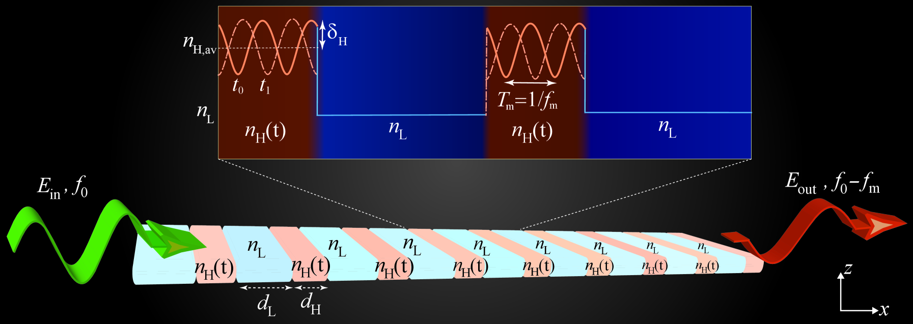
A Bragg grating is a periodic structure composed of alternating layers with high ($n_{\text{H}}$) and low ($n_{\text{L}}$) refractive indices, each having an optical thickness of $\lambda_{\text{B}}/4$ at the design wavelength $\lambda_{\text{B}}$. This quarter-wave condition ensures constructive interference of reflections from each interface, creating a photonic stopband centered at the Bragg frequency $\omega_{\text{B}}=2\pi c/\lambda_{\text{B}}$. When the refractive index of the Bragg grating layers is modulated in time, the system transforms from a passive filter into an active, time-variant medium capable of pure parametric frequency conversion in transmission. Consider the temporal Bragg grating in Fig. 1, where either the high-index or low-index layers experience sinusoidal temporal modulation:

$$n_{\text{L}}(t)=n_{\text{L},\text{av}}+\Delta_{\text{L}}\cos(\omega_{\text{m}}t+\phi_{\text{L}}),$$ (1a)

$$n_{\text{H}}(t)=n_{\text{H},\text{av}}+\Delta_{\text{H}}\cos(\omega_{\text{m}}t+\phi_{\text{H}})$$ (1b)

where $\Delta_{\text{L}}=\delta_{\text{L}}n_{\text{L}}$ and $\Delta_{\text{H}}=\delta_{\text{H}}n_{\text{H}}$, in which $\delta_{\text{L}}$ and $\delta_{\text{H}}$ are the temporal modulation amplitudes of the low and high index layers, respectively. In addition, $\omega_{\text{m}}=2\pi f_{\text{m}}$ is the modulation frequency, $\delta_{L},\delta_{H}\ll n_{\text{av}}$ are the modulation depths, and $\phi_{\text{L}},\phi_{\text{H}}$ are modulation phases whose adjustment controls the amplitude of the converted output. The temporal Bragg grating consists of $N$ periods, each with spatial period $\Lambda$. The total physical length of the structure is:

$$L=N\Lambda=N(d_{\text{H}}+d_{\text{L}}),$$ (2)

where $d_{\text{H}}=\lambda_{\text{B}}/(4n_{\text{H}})$ and $d_{\text{L}}=\lambda_{\text{B}}/(4n_{\text{L}})$ are the thicknesses of the high- and low-index layers, respectively. This length $L$ determines the interaction distance for parametric processes and is critical for achieving efficient conversion. Crucially, the inherent Bragg reflection at the stopband center frequency suppresses transmission at the input frequency. This suppression, combined with parametric coupling, enables the generation of a pure converted signal at the sideband frequencies. The temporal variation breaks time-translation symmetry, enabling photon energy conversion from the modulation pump at frequency $f_{\text{m}}$ to the optical signal at $f_{0}$ via $\hbar f_{\text{out}}=\hbar f_{0}\pm\hbar f_{\text{m}}$. The direction of conversion is determined by the modulated layer type: modulation of the high-index layers ($n_{\text{H}}$) predominantly generates a down-converted signal at $f_{-1}=f_{0}-f_{\text{m}}$, while modulation of the low-index layers ($n_{\text{L}}$) generates an up-converted signal at $f_{+1}=f_{0}+f_{\text{m}}$.

Figure 2: Space-time diagram of a temporal Bragg grating (up-conversion mode). The diagram tracks wave propagation through multiple spatial periods (horizontal axis $z$) and multiple modulation periods (vertical axis $ct$). Low-index layers are time-modulated (striped regions) and high-index layers are static (solid). Layer thicknesses $d_{\text{L}}$ and $d_{\text{H}}$ with corresponding transit times $\tau_{\text{L}}=n_{\text{L}}d_{\text{L}}/c$ and $\tau_{\text{H}}=n_{\text{H}}d_{\text{H}}/c$. Spatial period $\Lambda=d_{\text{L}}+d_{\text{H}}$. Modulation period $T_{\text{m}}=2\pi/\omega_{\text{m}}$ indicated by vertical spacing $cT_{\text{m}}$. Temporal scattering events recur with period $T_{\text{m}}$ within each modulated layer.

II-B Space-Time Diagram

To visualize the full complexity of wave propagation in a temporal Bragg grating, we construct a space-time diagram that tracks both spatial and temporal scattering events across multiple periods. Figure 2 presents this diagram for the case of low-index layer modulation, revealing the intricate interplay between periodic spatial boundaries and periodic temporal modulation. The diagram uses spatial coordinate $z$ on the horizontal axis and time $ct$ on the vertical axis, with light lines indicating wave propagation trajectories. The structure consists of alternating low-index ($n_{\text{L}}$, modulated) and high-index ($n_{\text{H}}$, static) layers with physical thicknesses $d_{\text{L}}$ and $d_{\text{H}}$, respectively. The transit time through each layer is:

$$\tau_{\text{L}}=\frac{d_{\text{L}}}{v_{\text{L}}}=\frac{n_{\text{L}}d_{\text{L}}}{c},$$ (3a)

$$\tau_{\text{H}}=\frac{d_{\text{H}}}{v_{\text{H}}}=\frac{n_{\text{H}}d_{\text{H}}}{c},$$ (3b)

where $v_{\text{L}}=c/n_{\text{L}}$ and $v_{\text{H}}=c/n_{\text{H}}$ are the group velocities (assuming negligible dispersion). These transit times determine the temporal spacing between successive scattering events within a single layer. Superimposed on these layer transit times is the modulation period $T_{\text{m}}=2\pi/\omega_{\text{m}}$, indicated by the vertical spacing $cT_{\text{m}}$. The diagram spans multiple modulation periods, revealing how the dynamics repeat with this temporal periodicity while accumulating phase.

In Fig. 2, one-headed arrows represent the standard spatial reflections and transmissions that occur at the boundaries between different material layers. A one-headed green arrow pointing toward the right indicates a spatial forward transmission, while one-headed red arrow pointing toward the left indicates a spatial backward-moving reflection. The two-headed arrows highlight the ”splitting” of waves at the temporal boundaries and represent temporal reflections and transmissions, where the wave is partially transmitted (continuing its spatial direction but shifting frequency) and partially ”time-reflected” (reversing its spatial direction at the moment of modulation). This distinction is crucial for interpreting the ”lattice” of paths in the diagram, as it shows how energy is distributed between different spatial and temporal sidebands. The modulation phase $\phi_{\text{L}}$ (implicit in the timing of these events) controls the coherent summation that determines conversion efficiency. At each interface between layers (vertical boundaries), conventional spatial scattering occurs. These events are labeled with the frequency $f_{0}$ (the incident frequency) and include

• Spatial reflections represented by wavenumbers $k_{0}^{\text{R1}}(0)$, $k_{0}^{\text{R1}}(2\tau_{\text{L}})$, $k_{0}^{\text{R2}}(\tau_{\text{L}}),\ldots$. Backward-propagating waves at $f_{0}$ generated at interfaces build the Bragg stopband that ultimately reflects the incident frequency.

• Spatial transmissions represented by wavenumbers $k_{0}^{\text{T2}}(0)$, $k_{0}^{\text{T3}}(\tau_{\text{L}})$, $k_{0}^{\text{T4}}(\tau_{\text{L}}+\tau_{\text{H}})$, $\ldots$ are forward-propagating waves at $f_{0}$ that continue into the next layer.

Within each modulated layer (low-index layers, indicated by the striped regions), the time-varying refractive index continuously generates new frequency components. These temporal scattering events are distributed throughout the layer volume, but for clarity we represent them as discrete events at representative instants. They include:

• Temporal reflections $k_{n}^{\text{R1}}(0)$, $k_{n}^{\text{R2}}(T_{\text{m}})$, $k_{n}^{\text{R2}}(T_{\text{m}}/2)$, $k_{n}^{\text{R2}}(3T_{\text{m}}/2),\ldots$ are polychromatic backward-propagating waves generated within the modulated layer and propagating leftward.

• Temporal transmissions $k_{n}^{\text{T2}}(0)$, $k_{n}^{\text{T2}}(T_{\text{m}}/2)$, $k_{n}^{\text{T2}}(T_{\text{m}})$, $k_{n}^{\text{T2}}(3T_{\text{m}}/2),\ldots$ represent polychromatic forward-propagating waves generated within the modulated layer and propagating rightward.

These temporal scattering events recur with period $T_{\text{m}}$ and create a vertical array of arrows spaced by $cT_{\text{m}}$ within each modulated layer. This visualizes the temporal periodicity of the modulation. While this diagram focuses on the full scattering dynamics, the frequency conversion outcome is determined by which of these many wave components interfere constructively at the output ports. The constructive interference condition involves the phase accumulated over multiple spatial and temporal periods, controlled by the modulation phase $\phi$. This phase appears implicitly in the timing of the temporal scattering events and can be tuned to maximize the output at the desired sideband frequency. The space-time diagram of Fig. 2 provides a complete visualization of the temporal Bragg grating dynamics, revealing the rich interplay between spatial periodicity (layer interfaces), temporal periodicity (modulation cycles), and the multiple time scales that govern wave propagation and frequency conversion.

II-C Origin of Layer-Dependent Frequency Conversion

The directional asymmetry in frequency conversion, up-conversion when modulating the low-index layers and down-conversion when modulating the high-index layers, finds its origin in the unique band structure of the quarter-wave Bragg grating and the associated Bloch mode profiles. At the Bragg frequency $\omega_{0}$, the electric field standing wave pattern within each unit cell is not uniformly distributed. Rather, it exhibits a distinct spatial asymmetry: for the lower band edge (immediately below the stopband), the field intensity peaks within the high-index layers, while for the upper band edge (immediately above the stopband), the field intensity peaks within the low-index layers [51]. This alternating field localization is a direct consequence of the quarter-wave condition and the contrasting refractive indices.

When a specific layer type is subjected to temporal modulation at frequency $\omega_{\text{m}}$, the time-varying refractive index acts as a parametric coupling mechanism that transfers energy from the incident wave at $\omega_{0}$ to adjacent Bloch modes. Crucially, the coupling strength is proportional to the field intensity within the modulated layer. Modulating the high-index layers, where the lower band-edge mode is concentrated, preferentially excites the down-converted sideband at $\omega_{0}-\omega_{\text{m}}$. Conversely, modulating the low-index layers, where the upper band-edge mode is concentrated, preferentially excites the up-converted sideband at $\omega_{0}+\omega_{\text{m}}$.

This intuitive Bloch mode picture is quantitatively captured by the phase-matching condition for distributed parametric conversion across $N$ periods. For efficient coherent buildup, the phase mismatch per period must satisfy

$$\Delta k_{\pm}\cdot\Lambda=2\pi m,\quad m\in\mathbb{Z},$$ (4)

where $\Delta k_{\pm}=\beta_{0}-\beta_{\pm}$ is the difference in propagation constants between the incident wave ($\beta_{0}$) and the sideband ($\beta_{\pm}\approx\beta_{0}\mp\omega_{\text{m}}/v_{\text{g}}$). The effective group velocity $v_{g}$ that appears in this expression is not simply the average of the layer velocities; rather, it is a weighted average that reflects the asymmetric field distribution. Because the field concentrates in the high-index layers, the effective group velocity is biased toward the slower velocity $c/n_{\text{H}}$. Consequently, the product $\Delta k_{\pm}\cdot\Lambda$ takes different magnitudes for the up- and down-converted sidebands

$$\Delta k_{+}\cdot\Lambda\approx-\frac{\omega_{\text{m}}}{v_{g}}\Lambda\quad\text{(up-conversion)},$$ (5a)

$$\Delta k_{-}\cdot\Lambda\approx+\frac{\omega_{\text{m}}}{v_{g}}\Lambda\quad\text{(down-conversion)}.$$ (5b)

The asymmetry in field distribution ensures that $|\Delta k_{+}\cdot\Lambda|$ is smaller when the low-index layers are modulated, favoring phase matching for up-conversion, while $|\Delta k_{-}\cdot\Lambda|$ is smaller when the high-index layers are modulated, favoring phase matching for down-conversion. Thus, the layer-dependent conversion direction emerges from a synergy of two fundamental mechanisms: (i) the spatial asymmetry of the Bloch modes in the static grating, which determines which sideband couples most strongly to the modulation, and (ii) the phase-matching condition arising from the periodic structure, which selects the sideband that can constructively interfere across multiple periods. This dual perspective, Bloch mode coupling and phase-matched distributed interaction, provides a complete physical picture of the directional frequency conversion observed in our temporal Bragg grating.

II-D Multi-Scattering Multi-Frequency Dynamics

Figure 3: Multiple-scattering diagram of a temporal Bragg grating operating in the up-conversion regime, where the low-index layers are time-modulated. An incident carrier at frequency ($f_{0}$) undergoes distributed frequency conversion within the modulated low-index regions, generating the up-converted sideband ($f_{+1}$). Constructive interference of the converted components across successive periods leads to the dominance of the ($f_{+1}$) harmonic at both output ports, while the original carrier is suppressed. The diagram illustrates the principal reflection and transmission pathways responsible for the distributed up-conversion process.

To understand the microscopic origin of the layer-dependent frequency conversion, we examine the multi-scattering dynamics within the temporal Bragg grating. Figure 3 presents space-time diagrams of the scattering processes for the Bragg grating possesing time-periodic low-index layers and static high-index layers. These diagrams demonstrate the distinct pathways by which the incident wave at frequency $f_{0}$ is converted to its sidebands through the interplay of spatial and temporal scattering events. When the low-index layers are time-modulated, the up-converted sideband $f_{+1}$ dominates both the transmitted and reflected ports. This striking behavior arises from two key factors. First, the Bloch mode profile of the quarter-wave stack at frequencies just above the stopband (the upper band edge) concentrates electric field energy in the low-index layers. Modulating these layers therefore couples strongly to the upper band-edge mode, preferentially generating $f_{+1}$. Second, and equally important, the frequency $f_{+1}$ lies outside the Bragg stopband. As the multi-scattering diagram shows, waves at $f_{+1}$ (bold arrows) propagate through the structure with minimal reflection at the layer interfaces. They transmit freely to the right and also emerge as a reflected wave to the left, having been generated within the modulated layers and scattered backward by the periodic structure. In contrast, the down-converted sideband $f_{-1}$ lies inside the stopband. Waves at $f_{-1}$ experience strong reflection at each interface and remain trapped within the structure, unable to contribute to either output port. The fundamental frequency $f_{0}$ (regular solid arrows) is also strongly reflected by the Bragg grating and is absent from both transmission and reflection. The result is bidirectional pure frequency conversion: both output ports carry only the up-converted frequency $f_{+1}$, with negligible power at $f_{0}$ or $f_{-1}$.

When the high-index layers are modulated (Fig. 4), the situation is symmetrically reversed. The Bloch mode at the lower band edge (frequencies just below the stopband) concentrates field energy in the high-index layers. Modulating these layers therefore couples strongly to the lower band-edge mode, preferentially generating the down-converted sideband $f_{-1}$. In this configuration, $f_{-1}$ lies outside the stopband and propagates freely through the structure, appearing in both transmission and reflection (bold arrows). The up-converted sideband $f_{+1}$ now lies inside the stopband, experiencing strong reflections and remaining trapped. Again, the fundamental $f_{0}$ is suppressed by the Bragg grating. The result is bidirectional pure down-conversion: both output ports carry only $f_{-1}$. The multi-scattering diagrams thus demonstrate a unified principle: the modulated layer selects which sideband is generated, and the Bragg stopband determines which sideband can escape. The Bloch mode asymmetry ensures that modulating low-index layers favors $f_{+1}$, while modulating high-index layers favors $f_{-1}$. The stopband then acts as a spectral filter, transmitting the favored sideband while trapping the other. Crucially, because the favored sideband is generated throughout the volume of each modulated layer and can propagate in both directions, it appears simultaneously in transmission and reflection, yielding efficient frequency conversion. This interplay between Bloch mode coupling (determining which sideband is generated) and stopband filtering (determining which sideband transmits) provides a complete and intuitive explanation for the layer-dependent, bidirectional frequency conversion observed in our full-wave simulations.

Figure 4: Multiple-scattering diagram of a temporal Bragg grating operating in the down-conversion regime, where the high-index layers are time-modulated. An incident wave at the carrier frequency ($f_{0}$) undergoes distributed frequency conversion within the modulated high-index regions, generating the down-converted sideband ($f_{-1}$). Constructive interference of the converted components across successive periods leads to the dominance of the ($f_{-1}$) harmonic at both output ports, while the original carrier is suppressed. The figure illustrates the principal reflection and transmission pathways responsible for the distributed frequency conversion process. The dominant sideband in a quarter-wave temporal Bragg grating is determined by the relative spatial phase between the temporal modulation profile and the carrier standing-wave distribution. Modulating alternating layers shifts the effective mixing profile by half a period, reversing the sign of the distributed phase-matched coupling coefficient and thereby switching the dominant conversion process between up- and down-conversion.

III Transmitted Fields

In this section, we develop a comprehensive transfer matrix formalism for temporal Bragg gratings. The approach captures both spatial periodicity (layer interfaces) and temporal periodicity (refractive index modulation), enabling quantitative prediction of the harmonic amplitudes in transmission and reflection. The refractive index of each layer may be static or time-modulated. We expand the electric field as a sum of harmonics

$$E(z,t)=\sum_{q=-\infty}^{\infty}E_{q}(z)e^{-i\omega_{q}t},$$ (6)

where $E_{q}(z)$ is the slowly varying amplitude of the $q$-th harmonic. In practice, for weak modulation, only the fundamental $q=0$ and first-order sidebands $q=\pm 1$ have significant amplitude, and we truncate the expansion to these three harmonics. Within a uniform layer, the propagation constant for harmonic $q$ depends on the layer type. For a layer with refractive index $n_{n}$ (with $n=L$ for low-index layers and $n=H$ for high-index layers), we have

$$k_{n,q}=\frac{\omega_{q}}{c}n_{n},$$ (7)

where $\omega_{q}=\omega_{0}+q\omega_{m}$ is the frequency of the $q$-th harmonic ($q=-1,0,+1$ for the three relevant harmonics). For a layer with time-varying index, the harmonic amplitudes satisfy coupled-mode equations derived from Maxwell’s equations. Applying the slowly varying envelope approximation (see Appendix A for a full derivation), we obtain

$$\frac{dE_{q}}{dz}=-ik_{n,q}E_{q}-i\kappa_{n}\left(e^{i\phi_{n}}E_{q-1}+e^{-i\phi_{n}}E_{q+1}\right),$$ (8a)

where the coupling strength reads

$$\kappa_{n}=\frac{\omega_{0}}{2c}\Delta_{n}.$$ (8b)

The first term on the right-hand side of Eq. (8a) represents phase accumulation, while the second term describes energy exchange between adjacent harmonics due to the temporal modulation. The modulation phase $\phi_{n}$ directly imprints on the coupling, providing a control knob for the phase of the generated sidebands. Equation (8a) is a system of coupled linear differential equations. For the three-harmonic truncation ($q=-1,0,+1$), we can write it in matrix form

$$\frac{d}{dz}\mathbf{E}=-i\mathbf{K}_{n}\mathbf{E},$$ (9a)

where $$\mathbf{E}=[E_{-1},E_{0},E_{+1}]^{T} \mathbf{K}_{n}$$ and the coupling matrix is

$$\mathbf{K}_{n}=\begin{bmatrix}k_{n,-1}&\kappa_{n}e^{-i\phi_{n}}&0\\ \kappa_{n}e^{i\phi_{n}}&k_{n,0}&\kappa_{n}e^{-i\phi_{n}}\\ 0&\kappa_{n}e^{i\phi_{n}}&k_{n,+1}\end{bmatrix}.$$ (9b)

The solution to Eq. (9a) over a layer of thickness $d_{n}$ is a matrix exponential

$$\mathbf{E}(z+d_{n})=\mathbf{P}_{n}\mathbf{E}(z),\quad\mathbf{P}_{n}=e^{-i\mathbf{K}_{n}d_{n}},$$ (10)

where for a static layer ($\kappa_{n}=0$), the coupling matrix is diagonal and the propagation matrix simplifies to

$$\mathbf{P}_{n}^{\text{(static)}}=\text{diag}\left(e^{-ik_{n,-1}d_{n}},e^{-ik_{n,0}d_{n}},e^{-ik_{n,+1}d_{n}}\right).$$ (11)

At an interface between layers $i$ and $j$, the refractive index changes discontinuously, but the modulation does not create new frequencies at the interface itself. The boundary conditions therefore couple harmonics only within the same frequency channel. The transmission and reflection coefficients for harmonic $q$ are the standard Fresnel coefficients for the static indices at frequency $\omega_{q}$

$$R_{q}^{ij} =\frac{n_{i}-n_{j}}{n_{i}+n_{j}}, T_{q}^{ij} =\frac{2n_{i}}{n_{i}+n_{j}}.$$ (12)

In matrix form, the interface transfer matrix is diagonal

$$\mathbf{T}^{ij}=\text{diag}\left(T_{-1}^{ij},T_{0}^{ij},T_{+1}^{ij}\right),$$ (13)

with the understanding that the reflected field is obtained by applying the reflection coefficients in a scattering matrix formulation. For the transfer matrix formalism propagating forward-going waves, we use the transmission coefficients as shown. A single unit cell of the temporal Bragg grating consists of a high-index layer followed by a low-index layer (or vice versa, depending on the stacking order). For a structure that begins and ends with high-index layers (typical for symmetric gratings), the unit cell transfer matrix is

$$\mathbf{M}=\mathbf{T}^{\text{HL}}\mathbf{P}_{\text{H}}\mathbf{T}^{\text{LH}}\mathbf{P}_{\text{L}},$$ (14)

where the order of multiplication corresponds to propagation from left to right. The specific form of $\mathbf{P}_{\text{L}}$ and $\mathbf{P}_{\text{H}}$ depends on which layer is modulated

• Case I — Low-index layers modulated: $\mathbf{P}_{\text{L}}=e^{-i\mathbf{K}_{\text{L}}d_{\text{L}}}$ (nondiagonal, with coupling $\kappa_{\text{L}}$), $\mathbf{P}_{\text{H}}=\mathbf{P}_{\text{H}}^{\text{(static)}}$ (diagonal).

• Case II — High-index layers modulated: $\mathbf{P}_{\text{H}}=e^{-i\mathbf{K}_{\text{H}}d_{\text{H}}}$ (nondiagonal, with coupling $\kappa_{\text{H}}$), $\mathbf{P}_{\text{L}}=\mathbf{P}_{\text{L}}^{\text{(static)}}$ (diagonal).

For a grating with $N$ identical periods, the total transfer matrix is simply the $N$-th power of the unit cell matrix

$$\mathbf{M}_{\text{tot}}=\mathbf{M}^{N}.$$ (15)

The output harmonic amplitudes for an incident wave at frequency $\omega_{0}$ are then

$$\begin{bmatrix}E_{-1}^{\text{out}}\\ E_{0}^{\text{out}}\\ E_{+1}^{\text{out}}\end{bmatrix}=\mathbf{M}_{\text{tot}}\begin{bmatrix}0\\ A_{0}^{\text{inc}}\\ 0\end{bmatrix},$$ (16)

where we have assumed incidence from the left with amplitude $A_{0}^{\text{inc}}$ and no incoming waves at the sideband frequencies.

The quarter-wave condition has important consequences for the carrier harmonic $q=0$. In each layer

$$k_{\text{L},0}d_{\text{L}}=\frac{\omega_{0}}{c}n_{\text{L}}d_{\text{L}}=\frac{\pi}{2},$$ (17a)

$$k_{\text{H},0}d_{\text{H}}=\frac{\omega_{0}}{c}n_{\text{H}}d_{\text{H}}=\frac{\pi}{2}.$$ (17b)

Thus, the propagation phase for the carrier through each layer is $e^{-i\pi/2}=-i$. This $\pi/2$ phase shift per layer is precisely the condition for constructive interference of reflections from each interface, creating the Bragg stopband centered at $\omega_{0}$. The carrier therefore experiences strong reflection and negligible transmission through an unmodulated grating.

For weak modulation ($\kappa_{n}d_{n}\ll 1$), we can obtain simple closed-form expressions for the sideband amplitudes. Treating the coupling terms in Eq. (9b) as perturbations, the first-order solution after $N$ periods reads

$$T_{+1}\approx-iN(\kappa_{n}d_{n})T_{0}^{\text{Bragg}}e^{i\phi_{n}},$$ (18a)

$$R_{+1}\approx-iN(\kappa_{n}d_{n})R_{0}^{\text{Bragg}}e^{i\phi_{n}},$$ (18b)

where $n=L$ for low-index modulation and $n=H$ for high-index modulation. Here, $T_{0}^{\text{Bragg}}$ and $R_{0}^{\text{Bragg}}$ are the transmission and reflection coefficients of the unmodulated Bragg grating at the carrier frequency $\omega_{0}$. For a high-contrast grating with many periods, $T_{0}^{\text{Bragg}}\approx 0$ and $R_{0}^{\text{Bragg}}\approx 1$.

Equations (18a) and (18b) pronounce several key features

• Linear growth with $N$: The sideband amplitude increases linearly with the number of periods, indicating distributed generation throughout the structure.

• Proportionality to modulation strength: The amplitude scales with $\kappa_{n}d_{n}\propto\Delta_{n}d_{n}$, allowing control via modulation depth.

• Phase control: The factor $e^{i\phi_{n}}$ shows that the modulation phase directly imprints on the generated sideband, providing a tuning knob.

• Bidirectional generation: Both transmission ($T_{+1}$) and reflection ($R_{+1}$) are nonzero, confirming that sidebands are generated in both directions, a key feature validated by full-wave simulations.

• Layer selectivity: The subscript $n$ indicates which layer type is modulated; the expressions for up-conversion ($+1$) and down-conversion ($-1$) are obtained by replacing $+1\rightarrow-1$ and adjusting the phase factor sign accordingly.

For down-conversion (high-index layers modulated), the corresponding expressions are

$$T_{-1}\approx-iN(\kappa_{\text{H}}d_{\text{H}})T_{0}^{\text{Bragg}}e^{-i\phi_{\text{H}}},$$ (19a)

$$R_{-1}\approx-iN(\kappa_{\text{H}}d_{\text{H}})R_{0}^{\text{Bragg}}e^{-i\phi_{\text{H}}},$$ (19b)

where the sign change in the phase factor ($e^{-i\phi_{\text{H}}}$ vs. $e^{i\phi_{\text{L}}}$) reflects the opposite frequency shift direction.

For stronger modulation or larger $N$, the first-order approximation breaks down, and we must account for the full coherent summation of contributions from all layers. As derived in Appendix B, the complete expressions are geometric series

$$T_{\pm}=\gamma A_{0}^{\text{inc}}e^{i\phi}\frac{(\tau_{\pm})^{N}-(\tau_{0})^{N}}{\tau_{\pm}-\tau_{0}},$$ (20a)

$$R_{\pm}=\gamma A_{0}^{\text{inc}}e^{i\phi}\frac{1-(\tau_{0}\rho_{\pm})^{N}}{1-\tau_{0}\rho_{\pm}},$$ (20b)

where $$\gamma \tau_{0} \tau_{\pm} \rho_{\pm} N$$ is the generation efficiency per layer, and are transmission coefficients at the fundamental and sideband frequencies, and is the reflection coefficient for the sideband propagating backward. These expressions reduce to Eqs. (18a) and (18b) in the limit of small or weak coupling, but also capture saturation and oscillation effects for stronger interactions.

A powerful feature demonstrated by Eqs. (20a) and (20b) is the dependence on the modulation phase $\phi_{n}$. For uniform modulation ($\phi_{n}=\phi$ constant), the phase appears as a global factor that does not affect the output power. However, by introducing a phase gradient across the structure, $\phi_{j}=\phi_{0}+j\Delta\phi$, the summation becomes:

$$T_{\pm}(\Delta\phi)=\gamma A_{0}^{\text{inc}}e^{i\phi_{0}}\sum_{j=1}^{N}(\tau_{0}e^{i\Delta\phi})^{j-1}(\tau_{\pm})^{N-j}.$$ (20c)

This is now a function of $\Delta\phi$, allowing the output amplitude to be tuned. The condition for resonant enhancement reads

$$\Delta\phi=\arg\left(\frac{\tau_{\pm}}{\tau_{0}}\right),$$ (20d)

which represents the temporal phase-matching condition, the analogue of the spatial Bragg condition but in the time domain. When satisfied, all contributions add in phase, maximizing the output. This phase sensitivity transforms the temporal Bragg grating into a temporal phased array, where electronic control of the modulation phases enables:

• Output amplitude tuning: Continuous adjustment of conversion efficiency.

• On/off switching: Complete cancellation at destructive phase combinations.

• Beam steering in time: Controlled direction of the converted wave in the time-frequency domain.

• Pulse shaping: Dynamic phase profiles for tailored temporal waveforms.

IV Results

Figure 5: Transmittance as a function of frequency for the passive (unmodulated) Bragg grating consisting of $N=8$ periods of alternating high-index ($n_{H}=2.5$) and low-index ($n_{L}=1.5$) layers, each satisfying the quarter-wave condition at the design frequency $f_{0}=150$ THz.

IV-A Transmission Spectrum of the Unmodulated Bragg Grating

Before introducing temporal modulation, we characterize the spectral response of the passive Bragg grating. Figure 5 shows the transmittance as a function of frequency for the unmodulated structure with $N=8$ periods. This transmission spectrum provides essential insight into the frequency-selective properties that underlie the device operation. The most prominent feature in Fig. 5 is a deep rejection notch centered at the design frequency $f_{0}=150$ THz. At this frequency, the transmittance drops below $10^{-3}$ (less than $-30$ dB), confirming that the incident wave lies at the center of a photonic stopband. This spectral selectivity is the key to the Bragg Frequency Convertor’s operation: the carrier $f_{0}$ is blocked, while the sidebands $f_{\pm 1}$ can transmit freely. When temporal modulation is applied, energy from the carrier is converted to these sidebands, which then emerge at the output. Outside the stopband, the transmittance exhibits oscillations as a function of frequency. These oscillations arise from Fabry-Perot resonances within the finite-length grating. At frequencies where an integer number of half-wavelengths fits within the total structure length $L=N\Lambda$, constructive interference enhances transmission, producing peaks that approach unity.

Figure 6: Full-wave simulation results for down-conversion mode (high-index layers modulated). The structure consists of a temporal Bragg grating with $N=8$, high-index layers modulated as $n_{\text{H}}(t)=2.5[1+0.12\cos(0.2\omega_{0}t-103.2^{\circ})]$; low-index layers are static. The incident wave at frequency $f_{0}=150$ THz enters from the left. All quantities are shown as functions of position $(x,y)$ within the grating. (a) Electric field $E_{z}$ at the incident frequency $f_{0}$. The field shows strong interference fringes on the left side, indicating reflection, with negligible field penetrating to the right side. (b) Time-averaged power flow at $f_{0}$. Power flows only on the left side (positive values near the input, negative values indicating reflected power), with essentially zero power transmission to the right. The carrier is fully reflected. (c) Time-averaged energy density at $f_{0}$. Energy is concentrated on the left side, with an exponentially decaying envelope into the structure, characteristic of evanescent penetration into a stop-band. The absence of energy on the right side confirms that the carrier does not transmit. (d) Electric field $E_{z}$ at the down-converted frequency $f_{-1}=120$ THz. Strong field appears on the right side, indicating transmission of the converted wave. (e) Time-averaged power flow at $f_{-1}$. Strong positive power flow is observed on the right side, confirming efficient transmission of the down-converted frequency. (f) Time-averaged energy density at $f_{-1}$. Energy is distributed throughout the structure, with significant density in the time-modulated high-index layers at the centre. The spatial modulation of energy density reflects the standing-wave pattern within the grating. (g) Output spectrum (transmittance) as a function of frequency, where the transmitted output is dominated by the down-converted frequency $f_{-1}$, with weak transmittance at $f_{0}$ and $f_{+1}$. (h) Transmittance at three main frequencies as a function of the modulation phase $\phi_{\text{H}}$.

IV-B Down Conversion

To further analyze the structure, we perform full-wave finite-difference time-domain (FDTD) simulations of the temporal Bragg grating. The design parameters are as follows. The Bragg structure consists of $N=8$ periods, comprising 8 high-index and 8 low-index layers, with a center frequency of $f_{0}=150$ THz corresponding to a Bragg wavelength $\lambda_{\text{B}}=2\;\mu\text{m}$ at the center of the stopband. The layers are time-modulated according to $n_{\text{L}}=1.5$ (static) and $n_{\text{H}}(t)=2.5[1+0.12\cos(\omega_{\text{m}}t-103.2^{\circ})$], where the modulation frequency $\omega_{\text{m}}=0.2\omega_{0}=0.4\pi\times 150$ THz (i.e., $f_{\text{m}}=0.2f_{0}=30$ THz) targets down-conversion to $f_{-1}=f_{0}-f_{\text{m}}=120$ THz.

Figures 6 to 6 show the response at the incident frequency of 150 THz. The electric field $E_{z}$ in Fig. 6 exhibits a clear standing-wave pattern on the left side of the structure, with nodes and antinodes characteristic of strong reflection. The field amplitude decays exponentially into the grating, which confirms that the fundamental frequency lies within the Bragg stopband created by the spatial periodicity. The time-averaged power flow at $f_{0}$ in Fig. 6 provides a quantitative measure of power transport, where positive values (red) indicate power flowing toward the structure, while negative values (blue) indicate reflected power flowing back toward the source. The power flow is confined entirely to the left side, with weak net power transmission to the right. The carrier is therefore completely reflected, consistent with the behavior of a high-contrast Bragg grating at the stopband center. The time-averaged energy density at $f_{0}$ in Fig. 6 shows a decaying envelope from left to right, where the absence of energy on the right side further confirms that the carrier does not transmit.

Figures 6 to 6 reveal a dramatically different behavior at the down-converted frequency. The electric field at $f_{-1}=120$ THz in Fig. 6 shows strong amplitude on the right side of the structure, indicating efficient transmission of the converted wave. The time-averaged power flow at $f_{-1}$ in Fig. 6 quantifies this frequency down-conversion, where strong positive power flow (red) appears on the right side, confirming efficient transmission of the down-converted frequency. The time-averaged energy density at $f_{-1}$ in Fig. 6 is distributed throughout the entire structure, where the energy density is strongest in the high-index layers near the center of the Bragg grating. The field builds up gradually from the input, reaching maximum amplitude in the middle periods before slowly decaying toward the output. This suggests that the down-converted wave experiences a resonant enhancement within the structure, with the central region acting as a cavity where forward- and backward-propagating components interfere constructively.

Figure 6 shows the transmitted power spectrum at the right (output) boundary. The output is dominated by a strong peak at the down-converted frequency $f_{-1}=120$ THz, with negligible power at $f_{0}$ and the up-converted frequency $f_{+1}=180$ THz. This confirms that the device performs pure, efficient down-conversion, where the carrier and other time-harmonics such as $f_{+1}$ and $f_{-2}$ are strongly suppressed, and only the desired sideband emerges. The absence of power at $f_{+1}$ validates the layer-selective nature of the conversion process—modulating the high-index layers preferentially couples to the lower band edge, generating $f_{-1}$ while suppressing $f_{+1}$.

A unique and powerful feature of the temporal Bragg grating is the ability to control the conversion efficiency via the modulation phase $\phi$. Figure 6 demonstrates this effect for the down-conversion mode, showing the transmitted power at the three relevant frequencies as $\phi_{\text{H}}$ is varied from $60^{\circ}$ to $110^{\circ}$. The power at $f_{-1}$ exhibits a clear sinusoidal variation with $\phi_{\text{H}}$, ranging from approximately $-2.52$ dB at the optimum phase ($\phi_{\text{H}}\approx 103.2^{\circ}$) to $-10.0$ dB at the minimum ($\phi_{\text{H}}\approx 60^{\circ}$). This $7.48$ dB tuning range demonstrates substantial phase control over the conversion efficiency. The transmitted power at the incident frequency $f_{0}$ remains strongly suppressed across the entire phase range, with values between $-20$ dB and $-37$ dB. This confirms that the Bragg stop-band effectively blocks the carrier regardless of the modulation state. The power at the up-converted frequency $f_{+1}$ is consistently below $-42$ dB across all phases, more than $30$ dB lower than the down-converted peak. This confirms the layer selectivity predicted, where modulating the high-index layers preferentially couples to the lower band edge, generating $f_{-1}$ while suppressing $f_{+1}$. The absence of any significant phase dependence for $f_{+1}$ further validates that this sideband is not resonantly enhanced and remains trapped within the stop-band regardless of the modulation phase.

Figure 7: Full-wave simulation results for up-conversion mode, where low-index layers modulated, that is, $n_{L}(t)=1.5[1+0.12\cos(0.2\,\omega_{0}t+\phi_{L})$ with $\phi_{L}=166.2^{\circ}$, and high-index layers are static. The incident wave at frequency $f_{0}$ enters from the left. All quantities are shown as functions of position $(x,y)$ within the grating. (a) Electric field $E_{z}$ at the incident frequency $f_{0}$. The field shows strong interference fringes on the left side, indicating reflection, with negligible field penetrating to the right side. This confirms that the fundamental frequency is blocked by the Bragg stopband regardless of which layer is modulated. (b) Time-averaged power flow at $f_{0}$. Power flows only on the left side (positive values near the input, negative values indicating reflected power), with essentially zero power transmission to the right. The carrier is fully reflected. (c) Time-averaged energy density at $f_{0}$. Energy is concentrated on the left side, with an exponentially decaying envelope into the structure, characteristic of evanescent penetration into a stopband. (d) Electric field $E_{z}$ at the up-converted frequency $f_{+1}$. Strong field appears on the right side, indicating transmission of the converted wave. (e) Time-averaged power flow at $f_{+1}$. Strong positive power flow is observed on the right side, confirming efficient transmission of the up-converted frequency. Negative power flow on the left indicates that the converted wave is also generated in the backward direction and emerges as reflection. (f) Time-averaged energy density at $f_{+1}$. Energy is distributed throughout the structure, with significant density on both sides, confirming that the up-converted wave propagates freely in both directions. (g) Output spectrum (transmittance) as a function of frequency, where the transmitted output is dominated by the up-converted frequency $f_{+1}$, with weak transmittance at $f_{0}$ and $f_{-1}$. (h) Dependence of transmittance on modulation phase $\phi_{L}$.

IV-C Up-Conversion

We now present full-wave simulation results for the complementary configuration where the low-index layers are time-modulated. The modulation parameters are $n_{\text{H}}=2.5$, $n_{\text{L}}(t)=1.5[1+0.12\cos(0.2\,\omega_{0}t+\phi_{\text{L}})]$, with the phase $\phi_{\text{L}}=166.2^{\circ}$ chosen to maximize conversion. The incident wave is again a continuous wave at $f_{0}=150$ THz entering from the left. Figure 7 presents the complete set of results, mirroring the structure of Fig. 6 for direct comparison.

Figures 7 to 7 show the response at the incident frequency. The electric field $E_{z}$ in Fig. 7 exhibits a standing-wave pattern on the left side, with only a small portion of the field penetrating to the right. The time-averaged power flow in Fig. 7 confirms small net transmission, where power flows only on the left side, with positive values indicating incident power and negative values indicating reflected power. The time-average energy density in Fig. 7 decays exponentially into the structure from the left, characteristic of evanescent penetration into a stopband. These results are essentially identical to those observed in the down-conversion case (Figs. 6-6, confirming that the carrier response is independent of which layer is modulated. The Bragg stopband formed by the spatial periodicity reflects $f_{0}$ regardless of the temporal modulation state.

Figures 7 to 7 reveal the up-converted response. The electric field at $f_{+1}$ in Fig. 7 shows strong amplitude on the right side, indicating efficient transmission of the up-converted wave. The time-averaged power flow at $f_{+1}$ in Fig. 7 quantifies this frequency up-conversion, where strong positive power flow (red) on the right confirms efficient transmission, while negative power flow (blue) on the left indicates that a large portion of the up-converted power is transmitted. The time-average energy density at $f_{+1}$ is shown in Fig. 7. A comparison of the energy density distributions in Figs. 7 and 6 reveals a subtle but important asymmetry that was not apparent at first glance. While both cases show field concentration in the high-index layers, the spatial location of this concentration differs significantly between up-conversion and down-conversion modes. At the up-converted frequency $f_{+1}$, the energy density is strongest in the high-index layers toward the right side of the Bragg grating. The field amplitude increases monotonically from left to right, reaching its maximum near the output facet. This indicates that the up-converted wave is generated progressively as the incident wave propagates through the structure, with each successive modulated layer adding to the forward-propagating wave. This asymmetry arises from the different phase-matching conditions for up- and down-conversion, combined with the dispersion of the periodic structure:

• Phase mismatch sign: For down-conversion ($f_{-1}$), the phase mismatch $\Delta k_{-}=\beta_{0}-\beta_{-1}$ is positive. This means that as the incident wave propagates, the generated down-converted wave accumulates phase relative to the pump. When this phase mismatch is compensated by the spatial periodicity (via the grating wavevector $K$), the interaction can be resonant, leading to energy exchange that peaks in the center of the structure, similar to second-harmonic generation in periodically poled crystals with optimal focusing.

• Up-conversion accumulation: For up-conversion ($f_{+1}$), the phase mismatch $\Delta k_{+}=\beta_{0}-\beta_{+1}$ is negative. The sign difference means that the up-converted wave builds up monotonically rather than resonantly, with maximum amplitude at the output where the interaction length is longest.

• Field overlap evolution: The overlap integral between the incident mode and the sideband mode evolves along the structure due to the changing relative phase. For down-conversion, this overlap is maximized in the center; for up-conversion, it increases monotonically.

Figure 7 shows the transmitted power spectrum at the right boundary. The incident power is at $f_{0}$. The output is dominated by a strong peak at the up-converted frequency $f_{+1}$, with only weak power at $f_{0}$ and the down-converted frequency $f_{-1}$. This confirms pure, efficient up-conversion, where the carrier is suppressed, and only the desired sideband emerges. The carrier suppression exceeds $11.6$ dB, and the unwanted down-converted sideband is more than $11$ dB below the peak. These metrics demonstrate that the device performs equally well for both conversion directions, with performance limited only by the modulation depth and number of periods. Figure 7 shows the transmitted power as a function of the modulation phase $\phi_{\text{L}}$, completing the characterization. The up-converted power $f_{+1}$ (blue circles) varies sinusoidally with $\phi_{\text{L}}$, exhibiting a clear maximum at $\phi_{\text{L}}\approx 166^{\circ}$ and a minimum at $\phi_{\text{L}}\approx 60^{\circ}$. The tuning range is approximately $12$ dB, and the carrier $f_{0}$ remains suppressed below $-11.6$ dB across all phases. The down-converted sideband $f_{-1}$ is consistently below $-11$ dB, confirming that modulating low-index layers selectively enhances up-conversion regardless of phase.

V Conclusion

This study introduced and demonstrated the Bragg Frequency Convertor, where temporal modulation of the high-index layers yields down-conversion, while modulation of the low-index layers yields up-conversion. The operating principle rests on an elegant synergy between spatial and temporal periodicities. The inherent Bragg stopband, arising from the spatial periodicity, strongly reflects the input carrier frequency, suppressing its transmission. Simultaneously, the temporal modulation generates sidebands at, and the Bloch mode structure of the quarter-wave stack ensures that the field concentrates in high-index layers at the lower band edge and in low-index layers at the upper band edge. Modulating a given layer therefore couples preferentially to the band-edge mode whose field peaks there, explaining the observed layer selectivity. The favored sideband lies outside the stopband and propagates freely through the structure. A comprehensive theoretical framework is developed based on coupled-mode theory and transfer matrix formalism. Full-wave finite-difference time-domain simulations have validated all key theoretical predictions. A particularly powerful feature demonstrated both theoretically and numerically is the control of conversion efficiency via the modulation phase. Extending this concept to phase gradients across the array would enable temporal phased-array operation, including beam steering in the time-frequency domain and programmable pulse shaping. As fabrication and modulation techniques continue to advance, this spatiotemporal architecture promises to become a versatile building block for future integrated photonic systems.

VI Appendix

VI-A Derivation of Coupled-Mode Equations

We derive the coupled-mode equations for a time-modulated layer starting from Maxwell’s equations. Consider a non-magnetic, lossless dielectric medium with a time-varying refractive index. For a one-dimensional structure with waves propagating in the $z$-direction and electric field polarized along $x$, the wave equation is

$$\frac{\partial^{2}E}{\partial z^{2}}-\frac{n^{2}(z,t)}{c^{2}}\frac{\partial^{2}E}{\partial t^{2}}=0.$$ (21)

For a time-modulated layer, the refractive index takes the form

$$n(z,t)=n_{0}+\Delta n\cos(\omega_{m}t+\phi),$$ (22)

where we have suppressed the $z$-dependence within the layer (the layer is uniform in space but time-varying). The modulation depth satisfies $\Delta n\ll n_{0}$.

VI-A1 Harmonic Expansion

Due to the time-periodic modulation, the electric field can be expanded in Floquet harmonics

$$E(z,t)=\sum_{q=-\infty}^{\infty}E_{q}(z)e^{-i\omega_{q}t},$$ (23)

where $\omega_{q}=\omega_{0}+q\omega_{m}$. The fundamental frequency $\omega_{0}$ is the incident frequency, which we assume is close to the Bragg frequency $\omega_{B}$. Substituting Eqs. (22) and (23) into the wave equation Eq. (21), we obtain

$$\sum_{q}\left[\frac{d^{2}E_{q}}{dz^{2}}e^{-i\omega_{q}t}+\frac{n^{2}(t)}{c^{2}}\omega_{q}^{2}E_{q}e^{-i\omega_{q}t}\right]=0.$$ (24)

VI-A2 Index Square Expansion

The square of the refractive index is

$$n^{2}(t) =\left(n_{0}+\Delta n\cos(\omega_{m}t+\phi)\right)^{2}$$

$$\approx n_{0}^{2}+2n_{0}\Delta n\cos(\omega_{m}t+\phi),$$ (25a)

where we have neglected the $$\Delta n^{2} \Delta n\ll n_{0}$$ term since . Writing the cosine in complex form

$$n^{2}(t)=n_{0}^{2}+n_{0}\Delta n\left(e^{i\phi}e^{i\omega_{m}t}+e^{-i\phi}e^{-i\omega_{m}t}\right).$$ (25b)

VI-A3 Frequency Mixing

When Eq. (25b) multiplies the harmonic sum in Eq. (24), terms like $e^{i\omega_{m}t}\cdot e^{-i\omega_{q}t}=e^{-i(\omega_{q}-\omega_{m})t}$ appear. This couples harmonic $q$ to harmonics $q-1$ and $q+1$. Specifically

$$n^{2}(t) \sum_{q}\omega_{q}^{2}E_{q}e^{-i\omega_{q}t}=n_{0}^{2}\sum_{q}\omega_{q}^{2}E_{q}e^{-i\omega_{q}t}$$

$$\quad+n_{0}\Delta ne^{i\phi}\sum_{q}\omega_{q}^{2}E_{q}e^{-i(\omega_{q}-\omega_{m})t}$$

$$\quad+n_{0}\Delta ne^{-i\phi}\sum_{q}\omega_{q}^{2}E_{q}e^{-i(\omega_{q}+\omega_{m})t}.$$ (26a)

Shifting indices in the sums ($q\rightarrow q+1$ in the second term, $q\rightarrow q-1$ in the third term) yields

$$n^{2}(t) \sum_{q}\omega_{q}^{2}E_{q}e^{-i\omega_{q}t}=\sum_{q}e^{-i\omega_{q}t}\Big[n_{0}^{2}\omega_{q}^{2}E_{q}$$

$$+n_{0}\Delta ne^{i\phi}\omega_{q+1}^{2}E_{q+1}+n_{0}\Delta ne^{-i\phi}\omega_{q-1}^{2}E_{q-1}\Big].$$ (26b)

VI-A4 Collecting Harmonics

Substituting Eq. (26b) into Eq. (24) and collecting coefficients of $e^{-i\omega_{q}t}$, we obtain for each harmonic $q$

$$\frac{d^{2}E_{q}}{dz^{2}}+\frac{\omega_{q}^{2}}{c^{2}}n_{0}^{2}E_{q}=-\frac{\omega_{q}^{2}}{c^{2}}n_{0}\Delta n\left(e^{i\phi}E_{q+1}+e^{-i\phi}E_{q-1}\right),$$ (27)

where we have used $\omega_{q\pm 1}\approx\omega_{q}$ in the coupling terms (since $\omega_{m}\ll\omega_{q}$), allowing us to replace $\omega_{q\pm 1}^{2}$ with $\omega_{q}^{2}$.

VI-A5 Slowly Varying Envelope Approximation

We now write the field as a forward-propagating wave with slowly varying amplitude

$$E_{q}(z)={E}_{q}(z)e^{ik_{q}z},$$ (28a)

where $k_{q}=\frac{\omega_{q}}{c}n_{0}$ is the propagation constant. Substituting into Eq. (27) and neglecting the second derivative of $\mathcal{E}_{q}$ (slowly varying approximation), we get

$$\begin{split}2ik_{q}\frac{d{E}_{q}}{dz}e^{ik_{q}z}=&-\frac{\omega_{q}^{2}}{c^{2}}n_{0}\Delta n\big(e^{i\phi}{E}_{q+1}e^{ik_{q+1}z}\\ &\qquad+e^{-i\phi}{E}_{q-1}e^{ik_{q-1}z}\big).\end{split}$$ (28b)

VI-A6 Phase Matching

The phase mismatch between harmonics is

$$\Delta k_{\pm}=k_{q}-k_{q\pm 1}=\mp\frac{\omega_{m}}{c}n_{0}.$$ (28c)

For typical modulation frequencies, $\Delta k_{\pm}d\ll 1$ over a single layer, so we can approximate $e^{i(k_{q\pm 1}-k_{q})z}\approx 1$ within the layer. This is the phase-matched approximation, valid when the layer thickness is much smaller than the beat length $2\pi/|\Delta k_{\pm}|$. With this approximation, Eq. (28b) reduces to

$$\frac{d{E}_{q}}{dz}=-i\frac{\omega_{q}}{2c}\Delta n\left(e^{i\phi}{E}_{q+1}+e^{-i\phi}{E}_{q-1}\right).$$ (28d)

VI-A7 Final Coupled-Mode Equations

Defining the coupling constant

$$\kappa=\frac{\omega_{0}}{2c}\Delta n,$$ (28e)

and returning to the original notation $E_{q}$ for the amplitude (now understood as the slowly varying envelope), we obtain the coupled-mode equations

$$\frac{dE_{q}}{dz}=-ik_{q}E_{q}-i\kappa\left(e^{i\phi}E_{q-1}+e^{-i\phi}E_{q+1}\right).$$ (28f)

The first term on the right-hand side, $-ik_{q}E_{q}$, which was omitted in the simplified derivation above, is recovered by noting that in Eq. (28a) we explicitly separated the rapid phase variation. When we work with the total field (not just the envelope), this term reappears. For consistency with the transfer matrix formulation, we retain it explicitly.

VI-A8 Extension to Multiple Layers

For a structure with multiple layers, each layer $j$ has its own refractive index $n_{j}$, modulation depth $\Delta n_{j}$, and modulation phase $\phi_{j}$. The coupled-mode equations become

$$\frac{dE_{q}}{dz}=-ik_{j,q}E_{q}-i\kappa_{j}\left(e^{i\phi_{j}}E_{q-1}+e^{-i\phi_{j}}E_{q+1}\right),$$ (28g)

where $k_{j,q}=\frac{\omega_{q}}{c}n_{j}$ and $\kappa_{j}=\frac{\omega_{0}}{2c}\Delta n_{j}$. This is the form used in the transfer matrix formulation of Sec. II.

VI-B Derivation of the Geometric Series Formulation

The geometric series expressions in Eqs. (20a) and (20b) arise from a systematic summation of all multi-scattering paths in the temporal Bragg grating. We derive them here by tracking the generation and propagation of sidebands through the periodic structure.

VI-B1 Physical Picture

Consider an incident wave of amplitude $A_{0}^{\text{inc}}$ at frequency $\omega_{0}$ entering from the left. As it propagates through the structure, each modulated layer generates waves at the sideband frequencies $\omega_{\pm}=\omega_{0}\pm\omega_{m}$. These generated waves then propagate to the output, accumulating phase and amplitude factors from transmission through the remaining layers.

The key insight is that each modulated layer contributes independently, and the total output is the coherent sum of these contributions. This is analogous to an array antenna, where each element radiates with a specific phase and amplitude.

VI-B2 Assumptions

The derivation rests on several assumptions that are valid for typical temporal Bragg gratings

1. Weak coupling: The generation efficiency per layer is small ($\gamma\ll 1$), so multiple generations within the same layer can be neglected (Born approximation).

2. No back-conversion: Once generated, sidebands do not strongly reconvert to other frequencies (valid for small modulation depth).

3. Linear propagation: Waves propagate linearly through the structure, with transmission and reflection coefficients that are independent of amplitude.

4. Periodicity: All layers are identical, with the same generation efficiency $\gamma$ and propagation coefficients $\tau_{0}$, $\tau_{\pm}$, and $\rho_{\pm}$.

VI-B3 Single Layer Contribution

Consider the $j$-th modulated layer (counting from the input, $j=1$ at the leftmost layer). The incident wave must first propagate through the preceding $j-1$ layers to reach this layer. Each of these layers transmits the fundamental frequency $\omega_{0}$ with coefficient $\tau_{0}$ (including both interfaces and propagation through the layer). Thus, the amplitude arriving at the $j$-th layer is

$$A_{0}^{(j)}=A_{0}^{\text{inc}}(\tau_{0})^{j-1}.$$ (29)

Upon reaching the $j$-th modulated layer, a fraction of the energy is converted to the sideband frequency. The generation efficiency per layer, $\gamma$, depends on the modulation depth $\Delta_{i}$, the field overlap, and the layer thickness. The generated sideband amplitude within the layer is given by

$$\Delta A_{\pm}^{(j)}=\gamma A_{0}^{(j)}e^{i\phi_{j}},$$ (30)

where $\phi_{j}$ is the modulation phase in the $j$-th layer. The phase factor $e^{i\phi_{j}}$ arises because the temporal modulation imprints its phase on the generated wave.

VI-B4 Propagation to the Output

Once generated, the sideband wave must propagate through the remaining $N-j$ layers to reach the output. Each of these layers transmits the sideband frequency with coefficient $\tau_{\pm}$. Thus, the contribution from the $j$-th layer to the transmitted output reads

$$\Delta T_{\pm}^{(j)}=\left[\gamma A_{0}^{\text{inc}}(\tau_{0})^{j-1}e^{i\phi_{j}}\right]\cdot(\tau_{\pm})^{N-j}.$$ (31a)

For the reflected output, the generated sideband must propagate backward through the same $j-1$ layers it already traversed (now in reverse direction). Each of these layers reflects or transmits the backward-propagating sideband. However, in a periodic structure, the backward propagation through $j-1$ identical layers is equivalent to forward propagation through the same number of layers with a reflection coefficient $\rho_{\pm}$ per layer. The contribution to reflection is therefore

$$\Delta R_{\pm}^{(j)}=\left[\gamma A_{0}^{\text{inc}}(\tau_{0})^{j-1}e^{i\phi_{j}}\right]\cdot(\rho_{\pm})^{j-1}.$$ (31b)

The factor $(\rho_{\pm})^{j-1}$ accounts for the cumulative reflection/backward transmission through the layers between the generation point and the input.

VI-B5 Coherent Summation Over All Layers

The total transmitted sideband amplitude is the sum over all $N$ modulated layers

$$T_{\pm}=\sum_{j=1}^{N}\Delta T_{\pm}^{(j)}=\gamma A_{0}^{\text{inc}}\sum_{j=1}^{N}(\tau_{0})^{j-1}(\tau_{\pm})^{N-j}e^{i\phi_{j}}.$$ (32a)

Similarly, the total reflected sideband amplitude is

$$R_{\pm}=\sum_{j=1}^{N}\Delta R_{\pm}^{(j)}=\gamma A_{0}^{\text{inc}}\sum_{j=1}^{N}(\tau_{0})^{j-1}(\rho_{\pm})^{j-1}e^{i\phi_{j}}.$$ (32b)

VI-B6 Uniform Modulation Case

For uniform modulation ($\phi_{j}=\phi$ constant), the phase factor can be taken outside the sum

$$T_{\pm}=\gamma A_{0}^{\text{inc}}e^{i\phi}\sum_{j=1}^{N}(\tau_{0})^{j-1}(\tau_{\pm})^{N-j},$$ (33a)

$$R_{\pm}=\gamma A_{0}^{\text{inc}}e^{i\phi}\sum_{j=1}^{N}(\tau_{0})^{j-1}(\rho_{\pm})^{j-1}.$$ (33b)

These are now standard geometric series. For the transmission sum, we have two cases

• If $\tau_{0}\neq\tau_{\pm}$, the sum is

  $$\sum_{j=1}^{N}(\tau_{0})^{j-1}(\tau_{\pm})^{N-j}=\frac{(\tau_{\pm})^{N}-(\tau_{0})^{N}}{\tau_{\pm}-\tau_{0}}.$$ (34a)

• If $\tau_{0}=\tau_{\pm}$, the sum simplifies to $N(\tau_{0})^{N-1}$.

  For the reflection sum, we have

  $$\sum_{j=1}^{N}(\tau_{0}\rho_{\pm})^{j-1}=\frac{1-(\tau_{0}\rho_{\pm})^{N}}{1-\tau_{0}\rho_{\pm}},$$ (34b)

  provided $\tau_{0}\rho_{\pm}\neq 1$.

Substituting these into Eqs. (33b) yields exactly the geometric series expressions

$$T_{\pm}=\gamma A_{0}^{\text{inc}}e^{i\phi}\frac{(\tau_{\pm})^{N}-(\tau_{0})^{N}}{\tau_{\pm}-\tau_{0}},$$ (35a)

$$R_{\pm}=\gamma A_{0}^{\text{inc}}e^{i\phi}\frac{1-(\tau_{0}\rho_{\pm})^{N}}{1-\tau_{0}\rho_{\pm}}.$$ (35b)

VI-B7 Connection to First-Order Perturbation

For small $N$ or weak coupling, we can expand these expressions. Using the binomial expansion $(\tau_{\pm})^{N}\approx 1+N\ln\tau_{\pm}$ and assuming $\tau_{\pm}\approx\tau_{0}\approx 1$ (low loss per layer), we obtain

$$T_{\pm}\approx\gamma A_{0}^{\text{inc}}e^{i\phi}\cdot N(\tau_{0})^{N-1}\approx\gamma A_{0}^{\text{inc}}e^{i\phi}N,$$ (36a)

$$R_{\pm}\approx\gamma A_{0}^{\text{inc}}e^{i\phi}\cdot N(\tau_{0}\rho_{\pm})^{N-1}\approx\gamma A_{0}^{\text{inc}}e^{i\phi}N,$$ (36b)

which translates to the first-order result $T_{\pm}\approx-iN(\kappa_{i}d_{i})T_{0}^{\text{Bragg}}e^{i\phi_{i}}$ in Eqs. (18a) and (18b) using $\gamma=-i\kappa_{i}d_{i}T_{0}^{\text{Bragg}}$ and note that $T_{0}^{\text{Bragg}}\approx 1$ for the incident wave propagation to each layer.

VI-B8 Physical Interpretation

The geometric series expressions have a clear physical interpretation:

• Numerator $(\tau_{\pm})^{N}-(\tau_{0})^{N}$: Represents the interference between two waves — one propagating entirely at the sideband frequency $(\tau_{\pm})^{N}$ and one propagating entirely at the fundamental $(\tau_{0})^{N}$ — after being generated at different layers.

• Denominator $\tau_{\pm}-\tau_{0}$: Accounts for the phase velocity mismatch between fundamental and sideband, which determines how quickly the contributions dephase.

• Factor $(\tau_{0}\rho_{\pm})^{N}$ in reflection: Shows that reflection builds up through repeated round trips between the generation point and the input.

• Global phase $e^{i\phi}$: Demonstrates that uniform modulation phase controls the overall phase of the output, while phase gradients (not shown here) control the interference condition.

References

- [1] S. Taravati and A. A. Kishk, “Space-time modulation: Principles and applications,” IEEE Microw. Mag., vol. 21, no. 4, pp. 30–56, 2020.
- [2] J. Sisler, P. Thureja, M. Y. Grajower, R. Sokhoyan, I. Huang, and H. A. Atwater, “Electrically tunable space–time metasurfaces at optical frequencies,” Nat. Nanotechnol, pp. 1–8, 2024.
- [3] S. Taravati and G. V. Eleftheriades, “Full-duplex reflective beamsteering metasurface featuring magnetless nonreciprocal amplification,” Nat. Commun., vol. 14, p. 4414, 2021.
- [4] S. Taravati, “Spatiotemporal photon blockade for nonreciprocal quantum absorption,” arXiv preprint arXiv:2409.08137, 2024.
- [5] S. Taravati and G. V. Eleftheriades, “4D wave transformations enabled by space-time metasurfaces: Foundations and illustrative examples,” IEEE Antennas Propagat. Mag., vol. 65, no. 4, pp. 61–74, 2023.
- [6] S. Taravati, “Designing space-time metamaterials: The central role of dispersion engineering,” arXiv preprint arXiv:2511.19541, 2025.
- [7] S. Taravati, A. A. Kishk, and G. V. Eleftheriades, “Finite-difference time-domain simulation of wave propagation in space-time-varying media: Derivation of schemes, extended framework, and illustrative examples,” IEEE Antennas Propagat. Mag., 2025.
- [8] R. K. Patel, S. Ramanathan, R. P. Jenkins, and M. J. Carter, “Photonic time crystals and time-varying electromagnetic metamatter: A new direction for ultrafast tunable photonic and microwave materials and devices,” Adv. Sci., p. e19790, 2026.
- [9] Z.-A. Chen, K. Liao, S.-B. Liu, Z.-C. Sun, Z.-Y. Huang, Z.-K. Liang, X.-H. Xie, and J.-P. Chang, “A novel wideband X-band amplifying metasurface,” IEEE Antennas Wirel. Propagat. Lett., 2026.
- [10] Y. Li, K. Duan, W. Zhao, J. Zhao, T. Jiang, K. Chen, and Y. Feng, “Tunable and reversible nonreciprocal transmission with cascaded time-modulated metasurface,” Laser Photonics Rev., vol. 20, no. 3, p. e02026, 2026.
- [11] S. Taravati, “Self-biased broadband magnet-free linear isolator based on one-way space-time coherency,” Phys. Rev. B, vol. 96, no. 23, p. 235150, Dec. 2017.
- [12] S. Taravati and G. V. Eleftheriades, “Lightweight low‐noise linear isolator integrating phase‐and amplitude‐engineered temporal loops,” Adv. Mater. Technol, p. 2100674, 2021.
- [13] I. Koutzoglou, S. Amanatiadis, and N. V. Kantartzis, “Robust and integrable time-varying metamaterials: A systematic survey and coherent mapping,” Nanomaterials, vol. 16, no. 3, p. 195, 2026.
- [14] S. Taravati, N. Chamanara, and C. Caloz, “Nonreciprocal electromagnetic scattering from a periodically space-time modulated slab and application to a quasisonic isolator,” Phys. Rev. B, vol. 96, no. 16, p. 165144, Oct. 2017.
- [15] N. Chamanara, S. Taravati, Z.-L. Deck-Léger, and C. Caloz, “Optical isolation based on space-time engineered asymmetric photonic bandgaps,” Phys. Rev. B, vol. 96, no. 15, p. 155409, Oct. 2017.
- [16] S. Taravati, “Giant linear nonreciprocity, zero reflection, and zero band gap in equilibrated space-time-varying media,” Phys. Rev. Appl., vol. 9, no. 6, p. 064012, Jun. 2018.
- [17] S. Taravati and G. V. Eleftheriades, “Full-duplex nonreciprocal beam steering by time-modulated phase-gradient metasurfaces,” Phys. Rev. Appl., vol. 14, no. 1, p. 014027, 2020.
- [18] S. Taravati, “Nonreciprocal entanglement of frequency-distinct qubits,” Adv. Quantum Technol., vol. 8, no. 10, p. e2500171, 2025.
- [19] H. Ö. Yılmaz, “Numerical investigation of a time-modulated lorentz-dispersive bianisotropic metasurface for nonreciprocal transmission and absorption,” Phys. Rev. B, vol. 112, no. 24, p. 245129, 2025.
- [20] S. Taravati and G. V. Eleftheriades, “Generalized space-time periodic diffraction gratings: Theory and applications,” Phys. Rev. Appl., vol. 12, no. 2, p. 024026, 2019.
- [21] A. Cullen, “A travelling-wave parametric amplifier,” Nat., vol. 181, no. 332, February 1958.
- [22] P. Tien and H. Suhl, “A traveling-wave ferromagnetic amplifier,” Proc. IEEE, vol. 46, no. 4, pp. 700–706, 1958.
- [23] S. Taravati and A. A. Kishk, “Dynamic modulation yields one-way beam splitting,” Phys. Rev. B, vol. 99, no. 7, p. 075101, Jan. 2019.
- [24] S. Taravati and G. V. Eleftheriades, “Programmable nonreciprocal meta-prism,” Sci. Rep., vol. 11, no. 1, pp. 1–12, 2021.
- [25] S. Taravati, “Temporal Bragg gratings: Broadband reconfigurable parametric amplifiers,” arXiv preprint arXiv:2512.22377, 2025.
- [26] S. Horsley and J. Pendry, “Traveling wave amplification in stationary gratings,” Phys. Rev. Lett., vol. 133, no. 15, p. 156903, 2024.
- [27] S. Taravati and C. Caloz, “Mixer-duplexer-antenna leaky-wave system based on periodic space-time modulation,” IEEE Trans. Antennas Propagat., vol. 65, no. 2, pp. 442–452, 2016.
- [28] S. Taravati and G. V. Eleftheriades, “Pure and linear frequency-conversion temporal metasurface,” Phys. Rev. Appl., vol. 15, no. 6, p. 064011, 2021.
- [29] S. Taravati, “Aperiodic space-time modulation for pure frequency mixing,” Phys. Rev. B, vol. 97, no. 11, p. 115131, 2018.
- [30] S. Taravati and G. V. Eleftheriades, “Microwave space-time-modulated metasurfaces,” ACS Photonics, vol. 9, no. 2, pp. 305–318, 2022.
- [31] S. Taravati, “Efficient nonreciprocal frequency conversion with space-time Josephson junction metasurfaces,” in 2024 54th European Microwave Conference (EuMC). IEEE, 2024, pp. 600–603.
- [32] F. Kovalev and I. Shadrivov, “Parametric metasurfaces for amplified upconversion of electromagnetic waves,” Appl. Phys. Lett., vol. 126, no. 26, 2025.
- [33] S. Taravati, “One-way absorption and isolation in space-time-periodic superconducting metasurfaces,” in 2024 Eighteenth International Congress on Artificial Materials for Novel Wave Phenomena (Metamaterials). IEEE, 2024, pp. 1–3.
- [34] S. Taravati and G. V. Eleftheriades, “Space-time medium functions as a perfect antenna-mixer-amplifier transceiver,” Phys. Rev. Appl., vol. 14, no. 5, p. 054017, 2020.
- [35] S. Taravati and C. Caloz, “Space-time modulated nonreciprocal mixing, amplifying and scanning leaky-wave antenna system,” in 2015 IEEE International Symposium on Antennas and Propagation & USNC/URSI National Radio Science Meeting. IEEE, 2015, pp. 639–640.
- [36] S. Taravati and A. A. Kishk, “Advanced wave engineering via obliquely illuminated space-time-modulated slab,” IEEE Trans. Antennas Propagat., vol. 67, no. 1, pp. 270–281, 2019.
- [37] S. Taravati, “Light transmission through space-time-modulated Josephson junction arrays and application to quantum angular-frequency beam multiplexing,” IEEE Trans. Antennas Propagat., 2025.
- [38] R. Sabri, M. M. Salary, and H. Mosallaei, “Broadband continuous beam-steering with time-modulated metasurfaces in the near-infrared spectral regime,” APL Photonics, vol. 6, no. 8, p. 086109, 2021.
- [39] S. Taravati, “Frequency-multiplexed millimeter-wave fault-tolerant superconducting qubits enabled by an on-chip nonreciprocal control bus,” arXiv preprint arXiv:2512.17588, 2025.
- [40] A. Othonos, “Fiber Bragg gratings,” Rev. Sci. Instrum., vol. 68, no. 12, pp. 4309–4341, 1997.
- [41] K. O. Hill and G. Meltz, “Fiber Bragg grating technology fundamentals and overview,” J. Light. Technol., vol. 15, no. 8, pp. 1263–1276, 2002.
- [42] C. Giles, “Lightwave applications of fiber Bragg gratings,” J. Light. Technol., vol. 15, no. 8, pp. 1391–1404, 2002.
- [43] M. Burla, L. R. Cortés, M. Li, X. Wang, L. Chrostowski, and J. Azaña, “Integrated waveguide Bragg gratings for microwave photonics signal processing,” Opt. Expr., vol. 21, no. 21, pp. 25 120–25 147, 2013.
- [44] J. Albert, L.-Y. Shao, and C. Caucheteur, “Tilted fiber Bragg grating sensors,” Laser & Photonics Reviews, vol. 7, no. 1, pp. 83–108, 2013.
- [45] M. Khalil, H. Sun, E. Berikaa, D. V. Plant, and L. R. Chen, “Electrically reconfigurable waveguide Bragg grating filters,” Opt. Expr., vol. 30, no. 22, pp. 39 643–39 651, 2022.
- [46] R. Rohan, K. Venkadeshwaran, and P. Ranjan, “Recent advancements of fiber Bragg grating sensors in biomedical application: a review,” J. Opt., vol. 53, no. 1, pp. 282–293, 2024.
- [47] T. A. La, O. Ülgen, R. Shnaiderman, and V. Ntziachristos, “Bragg grating etalon-based optical fiber for ultrasound and optoacoustic detection,” Nat. Commun., vol. 15, no. 1, p. 7521, 2024.
- [48] X. Xue, X. Han, L. Li, L. Min, D. You, and T. Guo, “Real-time monitoring of human breathing using wearable tilted fiber grating curvature sensors,” J. Light. Technol., vol. 41, no. 13, pp. 4531–4539, 2022.
- [49] X. Chen, X. Kang, Y. Gan, X. Zhang, N. Wang, Y. Zhu, J. Zhang, and X. Gan, “High-resolution, broadband on-chip spectrometer with tunable multi-mode waveguide Bragg gratings,” Opt. Expr., vol. 33, no. 17, pp. 35 385–35 399, 2025.
- [50] F. Brückerhoff-Plückelmann, T. Buskasper, J. Römer, L. Krämer, B. Malik, L. McRae, L. Kürpick, S. Palitza, C. Schuck, and W. Pernice, “General design flow for waveguide Bragg gratings,” Nanophotonics, vol. 14, no. 3, pp. 297–304, 2025.
- [51] P. Yeh and M. Hendry, “Optical waves in layered media,” 1990.