Ab Initio Adiabatic Potential Energy Surfaces and Non-adiabatic Couplings for O₃: Construction of Four State Diabatic Hamiltonian

ABSTRACT

We compute highly accurate first principle based ab initio adiabatic potential energy surfaces (PESs) using State-Averaged Multi-Configurational Self-Consistent Field (SA-MCSCF) followed by internally contracted Multi-Reference Configuration Interaction method incorporating fixed-reference Davidson corrections [ic-MRCI(Q)], where a full valence active space of 18 electrons in 12 orbitals and aug-cc-pVQZ basis set are employed for the low-lying four singlet electronic states of ozone ($\tilde{X}^{1}A^{\prime}$, $1~^{1}A^{\prime\prime}$, $1~^{1}A^{\prime}$ and $2^{1}A^{\prime\prime}$). It accurately reproduces the dissociation energies of ozone (1.101 eV) as well as the molecular oxygen (5.106 eV) along with vibrational frequencies of O₃ in comparison with experimental data. To ensure appropriate accuracy and proper convergence in the interaction as well as asymptotic regions, we (a) extend the number of electronic states in SA-MCSCF calculation (singlet as well as triplet and quintet); (b) systematically expand the active space [(12e,9o) $\rightarrow$ (18e,12o) $\rightarrow$ (24e,15o)] and basis set size (AVDZ $\rightarrow$ AV6Z $\rightarrow$ Complete Basis Set limit); (c) incorporate multi-reference character along with Davidson correction. Conical intersections between the adjacent electronic states (1-2, 2-3 and 3-4) are located at C_2v, D_3h as well as C_s geometries through the four-state adiabatic-to-diabatic transformation of non-adiabatic coupling terms (NACTs) computed at Coupled-Perturbed Multi-Configurational Self-Consistent Field (CP-MCSCF) method along the circular contours. Finally, we present: (a) ic-MRCI(Q) calculated minimum energy path of incoming oxygen to the diatom (O₂) is devoid of any “reef” feature; (b) NACTs and diabatic PES matrix elements as function of hyperangles ($\theta$, $\phi$) at a fixed hyperradius $\rho=4$ Bohr for a four state sub Hilbert space.

I. INTRODUCTION

Ozone (O₃) layer plays a vital role in stratospheric photochemistry shielding Earth from UV radiation ^{40, 49} and dissociates to molecular oxygen and atomic oxygen. Despite the apparent simplicity of the triatomic O₃ molecule, its spectroscopy and dynamics have remained challenging for decades. The persistent discrepancies⁷⁵ between predicted and observed low-temperature $\text{O}+\text{O}_{2}$ isotopic exchange rates are shown up from the negative temperature dependence in experiment. Moreover, the selective enrichment of heavy ozone isotopomers both in the atmosphere and laboratory settings deviates from the conventional mass-dependent isotope effect. This anomaly is known as the mass-independent fractionation (MIF) effect⁴³, which also remains unresolved. A major challenge in bridging theory and experiment lies in the absence of highly accurate first principle based global adiabatic/diabatic potential energy surfaces (PESs). In case of ozone, the complexity of ab initio calculations primarily arises from the slow convergence of correlation energies and nuclear gradients with respect to both the basis set size and the active space, owing to the strong coupling between adjacent electronic states. Over the past four decades, there have been continuous progresses primarily on the development of ground adiabatic PESs for ozone employing both semi-empirical and ab initio methods. Earlier works are summarized in Section S1 of the Supplementary Material (SM), whereas the following paragraphs focus on advancements in global adiabatic and diabatic PESs.

One of the earliest attempts to compute an ab initio global adiabatic ground state ($\tilde{X}^{1}A^{\prime}$) PES for ozone was made by Siebert et al. ⁷⁷ (SSB PES) using complete active space self consistent field (CASSCF) followed by multi-reference configuration interaction (MRCI) method with a relatively small active space of (12e,9o) and correlation-consistent polarized valence quadruple-zeta (cc-pVQZ) basis set. The SSB PES was generated by spline interpolation of approximately 5000 ab initio energies and successfully captured both the C_2v and D_3h minima, as well as the entrance/exit channel, $\text{O}_{2}(^{3}\Sigma_{g}^{-})$ + $\text{O}(^{3}P)$. On the other hand, the presence of a controversial artificial barrier (or reef) of 45 cm^-1 at the entrance/exit channel of minimum energy path (MEP) and an underestimated energy gap (D_e) of approximately 900 cm^-1 between the C_2v minima and the dissociation limit of ozone ($\text{O}_{2}(^{3}\Sigma_{g}^{-})$ + $\text{O}(^{3}P)$) was empirically modified (along its MEP) by Babikov et al. ⁶ following the calculations of Hernández-Lamoneda et al. ³⁶ and Fleurat-Lessard et al. ²⁵ The modified SSB PES was subsequently employed to investigate the metastable ⁶ and van der Waals states ^{32, 39} of O₃. Baloïtcha et al. ¹¹ developed diabatic PESs and transition dipole moment surfaces for the lowest five ${}^{1}A^{\prime}$ electronic states of ozone using contracted MRCI calculations with a slightly reduced aug-cc-pVTZ basis set. Those surfaces were used to locate several avoided crossings near the ground-state minimum and enabled quantum dynamics simulations that reproduced photodissociation cross sections and product state distributions. Schinke et al. studied ozone photodissociation in the wavelength range 200–1100 nm, covering the Hartley ⁶⁷, Huggins ⁶⁸, Chappuis ³⁰ and Wulf absorption bands ²⁹ using diabatic PESs constructed from ic-MRCI/aug-cc-pVTZ level of adiabatic PESs. Holka et al. ³⁸ validated earlier calculations of Schinke et. al. ^{77, 32, 68, 67, 30, 29} through a systematic investigation of electronic ground state PES of ozone using ic-MRCI singles and doubles (ic-MRCISD) as well as multireference averaged quadratic coupled cluster (ic-MR-AQCC) with a full valence CAS(18e,12o) and augmented correlation consistent basis sets extrapolated to the complete basis set (CBS) limit.

Later, Dawes et al. extensively studied the dissociation of O₃ using both basis set extrapolation ²⁰ and explicitly correlated methods ¹⁹, employing a full-valence complete active space, CAS(18e,12o) as reference. This calculation achieved an agreement within $\sim$30 cm^-1 for D_e by including spin-orbit coupling (SOC) and scalar relativistic effects. Moreover, it was showed that the controversial reef feature could be replaced by a smooth shoulder when the ground state ($\tilde{X}^{1}A^{\prime}$) was treated simultaneously with twelve (12) excited singlet states, six (6) of which correlate with the high-lying singlet dissociation limit. The resulting reef-free PES (DLLJG PES) qualitatively reproduced the negative temperature dependence of thermal rate constant for isotopic exchange reactions in terms of experimental trend. ^{47, 79} Lepers et al. ⁴⁶ developed a theoretical framework for long-range interactions of ozone and examined its spectroscopic and dynamical properties through electrostatic and van der Waals contributions. Tyuterev et al. ⁸³ developed an analytical ground-state PES (TKTHS PES) for ozone by correcting the non-vanishing “reef” feature of DLLJG surface at some geometry near the transition state along the MEP and computed thermal rate constants for the ¹⁸O + ³²O₂ $\rightarrow$ ³⁴O₂ + ¹⁶O exchange reaction ³⁴. Mankodi et al. ⁴⁸ constructed ab initio PESs using restricted active space self consistent field (RASSCF) followed by Complete Active Space Second-Order Perturbation Theory (CASPT2) with an active space of (12e,9o) and aug-cc-pVTZ basis set to compute collision-induced dissociation (CID) cross sections for the O₂ + O reaction by Quasi-Classical Trajectory (QCT) calculation. Powell et al. ⁶⁶ analyzed the O₂ + O $\rightleftharpoons$ O₃ reaction to examine the impact of various electronic structure methods on eliminating spurious reef features. Another PES is constructed by Varga et al. ⁸⁷ (PIP PES) for nine low-lying electronic states of ozone including singlet, triplet, and quintet using dynamical scaled external correlation (DSEC) corrected extended multi-state CASPT2 calculations to study the O(³P) + O₂(${}^{3}\Sigma_{g}^{-}$) collisions across a wide energy range. Alijah et al. ³ investigate the presence of topological phase in ozone, which affects highly excited rovibrational states. More recently, Egorov et al. ²² developed a long-range ab initio PES for ground state of ozone using extended CAS(24e,15o) at the ic-MRCI(Q) level combined with extrapolation to the complete basis set [CBS(56Z)] limit, where SOC among the nine (9) multiplet electronic states near dissociation channel ($\text{O}_{2}(^{3}\Sigma_{g}^{-})$ + $\text{O}(^{3}P)$) was incorporated to improve D_e. Wang et al. ⁸⁸ employed MRCI-based adiabatic PES (RKHS PES) to investigate the high-temperature rate of atom-exchange and dissociation dynamics of O₃.

For comprehensive understanding of ozone’s electronic structure, advanced computational methods are required to capture the strong electron-nuclear coupling. The identification and location of CIs provide essential insights into molecular processes. Over the past decades, Adhikari et al. formulated Beyond Born-Oppenheimer (BBO) equations for multi-state multi-mode systems and paved a practical way to implement such a complete theory in the field of spectroscopy and reactive scattering, where nonadiabatic coupling terms (NACTs) are incorporated from the first principles, enabling a unified and more accurate description of molecular ^{56, 27, 65, 35, 58} as well as chemical processes ^{50, 57, 64, 73}. While implementing such BBO based treatment to formulate diabatic Hamiltonian, it is necessary to demonstrate the path independence ⁷² of observables (cross section and rate constant) calculated from path dependent diabatic Hamiltonians and the existence of sub Hilbert space (SHS) ⁷⁰ for any specific molecular or chemical processes. So far, we have constructed BBO based diabatic Hamiltonian for three (H${}_{3}^{+}$⁵⁵, FH₂⁵³ and H₃²⁶) and four (HeH${}_{2}^{+}$⁶⁴ and at present, O₃) state SHS, where scattering calculations have been carried out^{28, 62, 26, 61} or will be performed on O₃ to explore the quantum effect on reaction attributes. While comparing our calculated cross section and rate constant for the above reactive processes with other theoretical results and experimental data, it would be quite interesting to examine the agreement/disagreement of the profiles (cross section/rate constant) obtained from the recently developed diabatic surfaces using CHIPR³³ and coupled adiabatic PESs employing Frobenius companion matrices using neural network based algorithm⁷⁶.

In this study, we investigate the intricacies of electronic structure calculations for ozone by exploring (a) various active spaces: CAS(12e,9o), (18e,12o) and (24e,15o) in combination with basis sets ranging from AVDZ $\rightarrow$ AV6Z; (b) the impact of different numbers of states in State Averaged Multi-Configurational Self-Consistent Field (SA-MCSCF) calculation to obtain global adiabatic PESs and in Coupled-Perturbed Multi-Configurational Self-Consistent Field (CP-MCSCF) method to evaluate nonadiabatic coupling terms (NACTs) of ozone and (c) internally contracted Multi-Reference Configuration Interaction method incorporating Davidson corrections [ic-MRCI(Q)] on the SA-MCSCF reference orbitals using converged CAS(18e,12o) and basis set (AVQZ) for the calculation of highly accurate global adiabatic PESs. The paper is structured as follows: Section II provides a brief overview on BBO theory and its equations for the construction of diabatic Hamiltonian from adiabatic quantities (PESs and NACTs). In Section III, we discuss on ab initio calculations for convergence of molecular parameters using different CASs, basis sets and various number of electronic states in SA-MCSCF followed by ic-MRCI(Q) calculation within Jacobi framework. Section IV explores the location of CIs by defining appropriate contours both at $\textit{C}_{2v}$ and $\textit{D}_{3h}$ geometries. Finally, Section V presents Diabatic PESs and couplings at a fixed hyperradius, $\rho$ = 4 Bohr. Section VI presents the conclusions and future perspective of this work.

II. THEORETICAL BACKGROUND

II.A. Adiabatic Representation of Schrödinger Equation

In the Born-Oppenheimer-Huang treatment, ^{14, 13} the total molecular wavefunction, {$\Psi(r,R)$}, for any $M$-dimensional electronic Hilbert Space can be expanded in terms of the electronic eigenfunctions ({$\xi_{i}$}s) with nuclear coordinate dependent coefficients known as adiabatic nuclear wavefunctions ({$\psi_{i}^{\rm ad}$}s) as:

$$\Psi(\textbf{r},\textbf{R})=\sum_{i=1}^{M}\psi_{i}^{\rm{ad}}(\textbf{R})\xi_{i}(\textbf{r};\textbf{R}),$$ (1)

where electronic and nuclear coordinates are denoted by r and R, respectively.

The total electron-nuclear Hamiltonian ($\hat{H}(\textbf{r},\textbf{R})$) is the sum of the nuclear kinetic energy operator ($\hat{T}_{\rm nuc}(\textbf{R})$) and the electronic Hamiltonian ($\hat{H}_{\rm{el}}(\textbf{r};\textbf{R})$).

$$\hat{H}(\textbf{r},\textbf{R})=\hat{T}_{\rm nuc}(\textbf{R})+\hat{H}_{\rm{el}}(\textbf{r};\textbf{R}),$$ (2)

The electronic eigenfunctions ({$\xi_{i}$}s) satisfy the electronic SE:

$$\hat{H}_{\rm{el}}(\textbf{r};\textbf{R})\xi_{i}(\textbf{r};\textbf{R})=u_{i}(\textbf{R})\xi_{i}(\textbf{r};\textbf{R}),\qquad\langle\xi_{i}|\xi_{j}\rangle_{\textbf{r}}=\delta_{ij}$$ (3)

where $u_{i}(\textbf{R})$ represents the adiabatic PESs.

Using the form of molecular wave function [Eq. (1)], the total electron-nuclear Hamiltonian [Eq. (2)] and the electronic eigenvalue equation [Eq. (3)], the molecular SE {$\hat{H}(\textbf{r},\textbf{R})\Psi(\textbf{r},\textbf{R})=E\Psi(\textbf{r},\textbf{R}$} on projection with the electronic eigenfunction ({$\xi_{i}$}) provides the kinetically coupled matrix form of adiabatic nuclear SE ¹⁰:

$$-\frac{\hbar^{2}}{2m}\left(\boldsymbol{\nabla}_{R}+\boldsymbol{\tau}\right)^{2}\psi^{\rm{ad}}+\left(U-E\right)\psi^{\rm{ad}}=0,$$ (4)

where $E$ signifies total energy, $U$ is the adiabatic potential energy matrix given by $U_{ij}=u_{i}\delta_{ij}$ and $\boldsymbol{\tau}$ defines the nonadiabatic coupling matrix (NACM) as given by:

$$\boldsymbol{\tau}_{ij}=\langle\xi_{i}|\boldsymbol{\nabla}_{R}\xi_{j}\rangle_{\textbf{r}}=-\langle\xi_{j}|\boldsymbol{\nabla}_{R}\xi_{i}\rangle_{\textbf{r}}=-\boldsymbol{\tau}_{ji},$$ (5)

and thereby, $\tau$ is a skew-symmetric matrix. On the other hand, while taking derivative on the electronic SE [Eq. (3)] with respect to nuclear coordinates ($\boldsymbol{\nabla}_{R}$) and projecting by electronic eigenfunctions ($\langle\xi_{i}|$), it appears that NACTs would be singular at point(s) or along seam(s) of degeneracy between electronic states as given below:

$$\boldsymbol{\tau}_{ij}=\frac{\langle\xi_{i}|\boldsymbol{\nabla}_{R}\hat{H}_{\rm{el}}|\xi_{j}\rangle_{\textbf{r}}}{u_{j}-u_{i}},$$ (6)

which is a reminiscent of Hellman-Feynman theorem ^{18, 24, 23}. Such singular terms not only introduce numerical inaccuracies but also could lead to non-conservation of energy ⁵⁹ in the adiabatic representation of SE. Therefore, it is necessary to transform the adiabatic SE [Eq. (4)] to another representation known as diabatic so that one can get rid of such singular terms.

II.B. Diabatic Schrödinger Equation

The adiabatic nuclear SE [Eq. (4)] can be transformed into the diabatic framework by carrying out an orthogonal transformation, $\psi^{\rm{ad}}=A\psi^{\rm{dia}}$,

$$\left(-\dfrac{\hbar^{2}}{2m}\nabla_{R}^{2}+W-E\right)\psi^{\rm{dia}}=0,$$ (7)

where $\psi^{\rm{dia}}$ denotes the diabatic nuclear wavefunction and $W$ is the diabatic potential energy matrix,

$$W=A^{\dagger}UA.$$ (8)

In order to obtain such adiabatic-to-diabatic representation of SE [Eq. (7)], the transformation matrix $A$ (also known as ADT matrix) must satisfy the following ADT condition, ^{7, 80, 73}

$$\boldsymbol{\nabla}_{R}A+\boldsymbol{\tau}A=0.$$ (9)

Since $\boldsymbol{\tau}$ is a skew-symmetric matrix, it can be depicted by manipulating [Eq. (9)] that the transformation matrix, $A$ has to be orthogonal by construction ($A^{\dagger}A=I$).

II.C. ADT Equations

Without losing generality, the ADT matrix ($A$) can be considered as a product of elementary rotation matrices constituted with mixing angles between the possible electronic states. ^{80, 2, 74, 52, 35} Therefore, for $M$ electronic states, the ADT matrix ($A$) can be considered as a product of $\Lambda=\ ^{M}C_{2}=\frac{M(M-1)}{2}$ elementary rotation matrices in $\Lambda!$ number of possible ways.

$$A=P_{n}\{A^{12}(\Theta_{12}).A^{13}(\Theta_{13})........A^{M-1,M}(\Theta_{M-1,M})\},\qquad n=1,...,\Lambda!,$$ (10)

where $P_{n}$ is the $n$th permutation between two rotation matrices and {$\Theta_{ij}$}s represent the ADT angles dependent on the nuclear coordinates. It may be noted that numerical solutions of any set of ADT equations originating from different permutations of elementary rotation matrices appear to be the same solution, {$\Theta_{ij}$}s. ⁶³

The matrix elements of any of the $A^{mn}(\Theta_{mn})$ matrices can be defined as:

$$\left[A^{mn}(\Theta_{mn})\right]_{mm}=\cos\Theta_{mn}=\left[A^{mn}(\Theta_{mn})\right]_{nn};\quad m\neq n$$ (11)

$$\left[A^{mn}(\Theta_{mn})\right]_{mn}=\sin\Theta_{mn}=-\left[A^{mn}(\Theta_{mn})\right]_{nm};\quad m\neq n$$

$$\text{and}\quad\left[A^{mn}(\Theta_{mn})\right]_{ij}=\delta_{ij};\quad\{i,j\}\neq\{m,n\}.$$

If the electronic sub-space ($N<<M$) exits for a specific molecular or chemical processes, two representative elementary rotation matrices for a 4-state SHS ($N=4$) are given by,

$$A^{12}(\Theta_{12})=\begin{pmatrix}\cos\Theta_{12}&\sin\Theta_{12}&0&0\\ -\sin\Theta_{12}&\cos\Theta_{12}&0&0\\ 0&0&1&0\\ 0&0&0&1\end{pmatrix},\hskip 8.5359ptA^{34}(\Theta_{34})=\begin{pmatrix}1&0&0&0\\ 0&1&0&0\\ 0&0&\cos\Theta_{34}&\sin\Theta_{34}\\ 0&0&-\sin\Theta_{34}&\cos\Theta_{34}\end{pmatrix}$$ (12)

With the model form of $A$ matrix [Eq. (10)-(12)] and the skew-symmetric form of NACM [Eq. (5)], the ADT condition [Eq. (9)] turns into the following six (6) first order coupled differential equations,

$$\boldsymbol{\nabla}\Theta_{ij}=\sum_{m=1}^{m=4}c^{(m)}\tau_{(m)},\qquad i=1,2,3;\hskip 2.84544ptj>i,$$ (13)

where the coefficients {$c^{(m)}$} are trigonometric functions of ADT angles {$\Theta_{ij}$}. The explicit form of the ADT equations and the diabatic PESs are presented in the section S3 and S4 of SM. The NACM elements ($\boldsymbol{\tau}_{ij}$) are calculated at every point of nuclear CS using the ab initio based CP-MCSCF method as implemented in the MOLPRO quantum chemistry package ⁹⁰ and then, employed to calculate the ADT angles ($\{\Theta_{ij}\}$) and the elements of the diabatic potential energy matrix ($\{W_{ij}\}$). Adhikari and co-workers developed a generalized algorithm, “ADT” ⁶³ by formulating the ADT quantities, namely the explicit form of ADT equations, NACTs and diabatic matrix elements through symbolic manipulation for $N$ dimensional SHS with $K$- degrees of freedom (DOF). This package can finally provide the numerical solution of ADT angles using the inputs of ab initio calculated NACTs to obtain diabatic Hamiltonian. A more comprehensive discussion of the theoretical framework of BBO can be found elsewhere.^{7, 80, 1, 73, 74, 8, 51, 21}

II.D. NACTs: Curl condition and Quantization

While exploring the existence of $N$-state SHS, we first numerically examined the validity of two conditions at each grid point or along a contour over the nuclear space as described below:

(a) Curl condition: When the cross derivatives on the scaler form of ADT equations [Eq. (9)] with respect to the pair of coordinates, $\theta$ and $\phi$ are carried out and subtracted from each other, the analytic continuation of ADT matrix elements $\Big(\frac{\partial^{2}A_{ij}}{\partial\theta\partial\phi}=\frac{\partial^{2}A_{ij}}{\partial\phi\partial\theta}\Big)$ provide the curl conditions (also referred to as the molecular field equation): ^{9, 7, 74}

$$F_{\theta\phi}^{ij}=\Big[\frac{\partial}{\partial\theta}\tau^{ij}_{\phi}-\frac{\partial}{\partial\phi}\tau^{ij}_{\theta}\Big]-\Big[(\tau_{\phi}\tau_{\theta})_{ij}-(\tau_{\theta}\tau_{\phi})_{ij}\Big]=0,$$ (14)

where $i,j$ are the two electronic states for a $N$-state SHS [$\{i,j\}\epsilon N$], $\tau_{\theta}^{ij}$ and $\tau_{\phi}^{ij}$ represent the scalar components of NACTs along $\theta$ and $\phi$ [$\theta$, $\phi$ represent hyperangles for a fixed hyperradius, $\rho$]. Such condition ensures that mathematical curl ($Z_{\theta\phi}^{ij}$) and the ADT curl ($C_{\theta\phi}^{ij}$) are equal:

$$Z_{\theta\phi}^{ij}=C_{\theta\phi}^{ij},$$ (15)

where

$$Z_{\theta\phi}^{ij} =\frac{\partial}{\partial\theta}\tau^{ij}_{\phi}-\frac{\partial}{\partial\phi}\tau^{ij}_{\theta},$$

$$C_{\theta\phi}^{ij} =(\tau_{\phi}\tau_{\theta})_{ij}-(\tau_{\theta}\tau_{\phi})_{ij}.$$

The existence of a chosen SHS at a specific point in the nuclear CS is verified using [Eq. (14) and Eq. (15)], confirming that the NACTs are free from any non-removable components. Consequently, the calculation of ADT matrix, which incorporates the effect of entire magnitude of NACTs for solving the ADT equations and for the construction of diabatic PES matrix, will be both theoretically “exact” and numerically “accurate”.

(b) Quantization of NACTs: As per the Cauchy’s residue theorem, a line integral along a circular contour encapsulating a singular function accumulates a value, an integer multiple of $\pi$. Since the NACTs could often be singular in the SHS, the following integral ⁹⁶ has an important role in the process of diabatization:

$$\int_{0}^{2\pi}\tau_{\phi}^{ij}(\theta)d\phi=0\hskip 5.69046ptor\hskip 5.69046ptn\pi\hskip 5.69046ptor\hskip 5.69046ptn.(2\pi),$$ (16)

where $n$ is the number of CIs enclosed by the contour defined by $\phi$ at fixed $\theta$. If the conditions given by Eq. (15) and Eq. (16) are satisfied at each specific grid point and over the circular nuclear coordinate, respectively, it can be assumed that the involved electronic states form a SHS. Otherwise, one need to expand the size of the SHS to verify those conditions until satisfied.

III. AB INITIO CALCULATIONS

Since the Jacobi coordinates are physically realizable and offer distinct advantages, we have generated the adiabatic PESs for capturing the features at various geometries and the NACTs for locating the CIs of the triatomic species, O₃ as defined by the variables $r$, $R$, and $\gamma$ as depicted in FIG. 1. The separation between the peripheral atoms of the O₂ molecule is denoted as $r$. The third O atom is presented at a distance $R$ from the center of mass of the diatom (O₂), where the angle between the vectors ($\textbf{r},\textbf{R}$) is denoted by $\gamma$. The side lengths from the third oxygen atom to the peripheral oxygen atoms are $R_{1}$ and $R_{3}$, where the separation between the two peripheral oxygen atoms is termed as $R_{2}$ (= $r$). All calculations have been performed using the MOLPRO quantum chemistry package ⁹⁰

FIG. 1: Schematic diagram of the Jacobi coordinates for the O₃ system.

III.A. Convergence of Active Space and Basis Set for ab initio calculation of O₃

The molecular parameters and energetics at selected geometries on the adiabatic ground-state PES of O₃ are computed systematically using different active spaces, basis sets and numbers of states in the SA-MCSCF and thereafter, ic-MRCI(Q) calculations, as summarized in Table 1 and 2, respectively. The “convergence” as well as “accuracy” of such parameters and the overall smoothness of the adiabatic PESs are examined by: (a) exploring three variants of CASs, namely, (i) outer valence CAS(12e,9o) using only the 2p orbitals; (ii) full valence CAS(18e,12o) including the 2s and 2p orbitals; (iii) extended CAS(24e,15o) including core and valence orbitals (1s, 2s and 2p); (b) expanding the basis set (aug-cc-pVXZ, X = 2, 3, .., 6) from AVDZ to AV6Z and eventually to the complete basis set (CBS) limit; (c) extending the number of singlet states in the SA-MCSCF calculation (3S $\rightarrow$ 13S) and also with three triplet (3T) and three quintet (3Q) states along with three singlet states (3S); and (d) finally, incorporating multireference effects along with Davidson correction. These systematic refinements improve substantially the accuracy of the molecular parameters as well as smoothness of adiabatic PESs within computational feasibility.

III.A.1. SA-MCSCF

For the first two variants of CAS [(12e,9o) and (18e,12o)] with AVDZ basis set, 3S-SA-MCSCF to 7S-SA-MCSCF calculations depict that the higher CAS(18e,12o) could able to provide not only improved molecular parameters at different geometries but also quite smooth adiabatic PESs both at the interaction and asymptotic regions. The additional improvement obtained by using a larger active space CAS(24e,15o) with the same basis set (AVDZ) and upto 7S-SA-MCSCF calculation is negligibly “small” while being computationally more demanding. On the process of averaging over increasing number of states, it appears that both 7S-SA-MCSCF and 13S-SA-MCSCF calculations with CAS(18e,12o) using AVDZ basis set provide smooth adiabatic PESs, but the energetics at specific geometries are not improved significantly. Subsequently, calculations using higher basis sets (AVDZ $\rightarrow$ AV6Z) have been carried out at the 7S-SA-MCSCF level with CAS(18e,12o) for betterment of energetics. In contrast, for the larger active space CAS(24e,15o), the 4S-SA-MCSCF calculations can produce sufficiently smooth adiabatic PESs, where such calculation (4S-SA-MCSCF) for higher basis set (AVDZ $\rightarrow$ AV6Z) can improve energetics incrementally. Although the 4S-SA-MCSCF calculations with CAS(24e,15o) yield converged geometrical parameters and energetics at the AVQZ basis set, the 7S-SA-MCSCF calculations with CAS(18e,12o) achieve convergence in geometrical parameters and energetics only around the interaction region (near C_2v and D_3h minima) at the AVQZ level. For the latter active space [CAS(18e,12o)], the energetics of the B1 (O₃ $\rightarrow$ O₂ + O) and B2 (O₂ $\rightarrow$ O + O) dissociation processes increase incrementally with increasing basis set size (AVDZ $\rightarrow$ AV6Z). Nevertheless, nearly converged or converged results for B1 and B2 processes obtained with CAS(18e,12o)/7S-SA-MCSCF and CAS(24e,15o)/4S-SA-MCSCF calculations using the AV6Z basis set, are still far away from the experimentally measured values ^{4, 37}.

The convergence of molecular parameters and energetics was further examined by including three triplet (3T) and three quintet (3Q) states in addition to three singlet (3S) states in the SA-MCSCF calculations for both CAS(18e,12o) and CAS(24e,15o). Although the resulting PESs are sufficiently smooth in both cases, the predicted geometries and energetics do not show any improvement compared to singlet only approaches.

The progressive convergence of molecular parameters at different geometries as well as energetics for various processes are depicted in Table 1 with the change of active space, basis set, and number of states involved in SA-MCSCF approaches with same as well as different spin states.

Table 1: SA-MCSCF computed energy (eV) differences relative to O + O₂ and other configurations of O₃ on the ground ($\tilde{X}^{1}A^{\prime}$) adiabatic PES for various active spaces and basis sets.

Active Space	Basis Set	States	$\Delta E_{1}^{a}$	$\Delta E_{2}^{b}$	$\Delta E_{3}^{c}$	$\textit{C}_{2v}$ ($R_{1},\alpha$)d	$\textit{D}_{3h}$ ($R_{1}$)d	O2 ($R_{2}$)d
(12e, 9o)	AVDZ	3S	1.52	0.12	3.74	1.28, 115.2	1.47	1.22
		4S	0.32	0.03	2.63	1.28, 115.2	1.47	1.22
		7S	0.29	-1.29	3.87	1.28, 115.2	1.47	1.22
	AVDZ	3S	1.43	0.25	3.85	1.28, 115.2	1.47	1.22
		4S	1.41	0.17	3.88	1.28, 115.2	1.47	1.22
		7S	1.45	0.12	3.92	1.29, 116.6	1.48	1.22
		13S	1.47	0.10	3.94	1.29, 116.6	1.48	1.22
(18e, 12o)		3S+3T+3Q	1.41	0.04	3.84	1.30, 116.5	1.47	1.22
	AVTZ	7S	1.34	0.24	4.05	1.29, 116.6	1.47	1.22
	AVQZ	7S	1.37	0.26	4.04	1.29, 116.8	1.47	1.22
	AV5Z	7S	1.36	0.29	4.08	1.29, 116.8	1.47	1.22
	AV6Z	7S	1.36	0.40	4.09	1.29, 116.8	1.47	1.22
	AVDZ	3S	1.43	0.25	3.88	1.28, 115.2	1.47	1.22
		4S	1.43	0.17	3.91	1.29, 115.8	1.46	1.22
		7S	1.46	0.12	3.91	1.30, 115.9	1.46	1.22
		3S+3T+3Q	1.41	0.04	3.85	1.31, 116.5	1.47	1.22
(24e, 15o)	AVTZ	4S	1.29	0.27	4.03	1.29, 116.7	1.47	1.22
	AVQZ	4S	1.33	0.27	4.06	1.29, 116.8	1.47	1.22
	AV5Z	4S	1.33	0.27	4.08	1.29, 116.8	1.47	1.22
	AV6Z	4S	1.33	0.28	4.07	1.29, 116.8	1.47	1.22
Expt.	–	–	–	1.14e	5.12 89	1.27, 116.7 4	–	1.21 37

^a $E(\textit{D}_{3h})-E(\textit{C}_{2v})$
^b $E(O_{2}+O)-E(\textit{C}_{2v})$
^c $E(O+O+O)-E(O_{2}+O))$
^d $R_{1},R_{2},R_{3}$: $O_{1}-O_{2}$, $O_{2}-O_{3}$ and $O_{3}-O_{1}$ distances (Å), respectively; $\alpha$: $\angle O_{2}-\hat{O_{1}}-O_{3}$(deg).
^e experimental dissociation energy (D₀) = (1.0617 $\pm$ 0.0004 eV) ⁶⁹ with the zero point energies (ZPEs) of O₃ (0.1771 $\pm$ 0.0002 eV) ²² and O₂ (0.0965 $\pm$ 10^-5 eV) ²².

III.A.2. ic-MRCI(Q)

Since the molecular parameters for defining global adiabatic PESs at the interaction as well as asymptotic region are crucially important, it appears various SA-MCSCF calculated results even with larger active spaces [CAS(18e,12o) and CAS(24e,15o)] as well as with increasing basis sets (AVDZ $\rightarrow$ AV6Z) remain far away from the available experimental values, namely, dissociation energy of B1 (O₃ $\rightarrow$ O₂ + O) and B2 (O₂ $\rightarrow$ O + O) processes. On the other hand, as the precise description of bond dissociation processes demands the inclusion of dynamic correlation, we carry out internally contracted multi-reference configuration interaction calculations with fixed-reference Davidson correction [ic-MRCI(Q)] ^{91, 42} for four low-lying electronic states, where those four (low-lying) reference states are taken from (i) 7S-SA-MCSCF with CAS(18e,12o) and (ii) 4S-SA-MCSCF with CAS(24e,15o), using different basis sets. The resulting geometrical parameters as well as energetics show significant improvement and show in good agreement with previous theoretical ^{44, 93, 5, 60, 77, 38, 46, 19, 83, 48, 87, 22} and experimental measurements ^{4, 37} (see Table 2).

The ic-MRCI(Q) calculations show: (a) The geometrical parameters near the vicinity of C_2v and D_3h minima as well as the energy separation between these two minima remain nearly unchanged compared to the SA-MCSCF results, which is due to the similar types of correlation energies at those geometries (see Table 3); (b) Using AVQZ basis set, the energy gap between the C_2v minimum and the asymptote of $\text{O}_{2}(^{3}\Sigma_{g}^{-})$ + $\text{O}(^{3}P)$ channel improves significantly by reaching 1.101 eV with CAS(18e,12o), compared to 0.253 eV obtained at the 7S-SA-MCSCF level. For the extended CAS(24e,15o), this gap increases to 1.110 eV relative to the 4S-SA-MCSCF value (0.270 eV), where the experimentally measured value ⁴ is 1.144 eV. Moreover, the dissociation energy of molecular O₂ is found to be 5.106 eV with CAS(18e,12o), compared to the corresponding 7S-SA-MCSCF calculated value, 4.04 eV. Again, for the larger CAS(24e,15o), such dissociation energy is 5.145 eV, compared to 4.06 eV obtained at the 4S-SA-MCSCF level. The dissociation energy for B2 process calculated with CAS(18e,12o) and AVQZ basis (5.106 eV) shows slightly closer agreement with experiment (5.117 eV) ⁸⁹ compare to the corresponding case with CAS(24e,15o) and AVQZ basis (5.145 eV); (c) Numerical instabilities of electronic structure calculations using 7S-SA-MCSCF followed by ic-MRCI(Q) approaches become progressively more pronounced at large $R(\geq 7$–8 bohr) for the CAS(18e,12o), which makes difficult to obtain reliable dissociation energies in this region for both the B1 and B2 processes. To overcome this issue, a long-range correction is introduced using the methodology proposed by Tyuterev et al. ⁸³, where at present, the 7-SA-MCSCF calculations are first performed using the CAS(12e,9o) and therein, both the 1s and 2s orbitals are optimized with active 2p orbitals. The resulting orbitals are re-optimized at the 7S-SA-MCSCF level using CAS(18e,12o) within the frozen-core approximation (i.e., 1s orbitals kept frozen). These reference orbitals are employed in ic-MRCI(Q) calculations using CAS(18e,12o) with frozen-core approximation. On the contrary, it appears that such treatment is not required for the CAS(24e,15o) calculations; (d) Upon further increase of basis set size [AVQZ $\rightarrow$ AV5Z $\rightarrow$ AV6Z], the dissociation energy for the B₁ process continues to improve [1.101 $\rightarrow$ 1.119 $\rightarrow$ 1.130 eV for CAS(18e,12o) and 1.110 $\rightarrow$ 1.130 $\rightarrow$ 1.136 eV for CAS(24e,15o)] and approaches the experimental value (1.144 eV). However, the higher basis sets [AVQZ $\rightarrow$ AV5Z $\rightarrow$ AV6Z] tend to “slightly” overestimate the experimental value of O₂ dissociation energy, 5.117 eV in the B₂ process, yielding values of 5.106 $\rightarrow$ 5.139 $\rightarrow$ 5.147 eV for CAS(18e,12o) and 5.145 $\rightarrow$ 5.183 $\rightarrow$ 5.192 eV for CAS(24e,15o). For the CBS extrapolation based on both the CAS(18e,12o) and CAS(24e,15o), the AVQZ $\rightarrow$ AV5Z $\rightarrow$ AV6Z $\rightarrow$ CBS(56Z) scheme is adopted, where long-range correction is incorporated for the former CAS(18e,12o) at large $R$ as described above ⁸³. The extrapolation to the CBS limit is made using the E_cbs + A/X³ functional, where E_cbs corresponds to the total energy (reference + correlation). This strategy reproduces the experimental dissociation energy for the B1 process (O₃ $\rightarrow$ O₂ + O) reasonably well, but “slightly” overestimates the experimental value of B2 process (O₂ $\rightarrow$ 2O). (e) From the analysis on computational time and memory requirement (see Table S1 of SM), it is observed that the CAS(18e,12o) and AVQZ basis set is the optimal one for generating multi-state global adiabatic PESs, which not only provide closely “accurate” description of both the interaction region as well as the asymptotic dissociation limits, but also computationally feasible. Although the CAS(24e,15o) increases the “accuracy” of the PES, but it is highly computationally demanding.; (f) To further assess the accuracy of the PESs, vibrational calculations are performed using the CAS(18e,12o) with different basis sets, as summarized in Table 4. These calculations yield converged equilibrium geometries ($r_{e}$, $\alpha_{e}$) and harmonic (vibrational) frequencies ($\omega_{i}$s) of ozone for the CAS(18e,12o) with AVQZ basis set and provided results that are in closest agreement with the available experimental ⁴⁵ and other theoretical data ^{38, 84, 83}.

Table 2: Comparison of molecular parameters and energetics at specific geometries on the ground-state adiabatic ($\tilde{X}^{1}A^{\prime}$) PES of O₃, computed at the ic-MRCI(Q) level using different active spaces and basis sets, together with other theoretical and experimental data.

References	$\Delta E_{1}^{a}$	$\Delta E_{2}^{b}$	$\Delta E_{3}^{c}$	$\textit{C}_{2v}$ ($R_{1},\alpha$)d	$\textit{D}_{3h}$ ($R_{1}$)d	O2 ($R_{2}$)d
Müller et al. 60	1.279	1.062	–	1.267, 117.2	1.438	–
Siebert et al. 77	1.340	1.027	–	1.275, 116.8	1.441	–
Holka et al. 38	–	1.110	–	1.270, 116.8	–	1.203
Dawes et al. 19	1.330	1.160	–	1.270, 116.8	1.440	–
Tyuterev et al. 83	–	1.119	–	1.275, 116.8	–	1.206
Varga et al. 87	1.190	1.160	–	1.270, 119.4	1.430	1.210
Egorov et al. 22	–	1.143	–	1.269, 116.9	–	1.205
Present Worke
CAS (18e,12o)
AVDZ	1.467	0.722	4.635	1.293, 116.6	1.483	1.217
AVTZ	1.342	1.019	5.013	1.288, 116.8	1.470	1.217
AVQZ	1.365	1.101	5.106	1.288, 116.8	1.470	1.217
AV5Z	1.369	1.119	5.139	1.288, 116.8	1.467	1.217
AV6Z	1.369	1.130	5.147	1.288, 116.8	1.466	1.217
CBS(56Z)	1.370	1.143	5.155	1.288, 116.8	1.466	1.217
CAS (24e,15o)
AVTZ	1.372	1.088	5.106	1.290, 116.7	1.470	1.217
AVQZ	1.379	1.110	5.145	1.284, 115.3	1.470	1.217
AV5Z	1.380	1.130	5.183	1.284, 115.3	1.470	1.217
AV6Z	1.380	1.136	5.192	1.284, 115.3	1.470	1.217
CBS(56Z)	1.380	1.142	5.201	1.288, 116.8	1.466	1.217
Expt.	–	1.144f	5.117 89	1.273, 116.8 4	–	1.207 37

^a $E(\textit{D}_{3h})-E(\textit{C}_{2v})$
^b $E(O_{2}+O)-E(\textit{C}_{2v})$
^c $E(O+O+O)-E(O_{2}+O))$
^d $R_{1},R_{2},R_{3}$: $O_{1}-O_{2}$, $O_{2}-O_{3}$ and $O_{3}-O_{1}$ distances (Å), respectively; $\alpha$: $\angle O_{2}-\hat{O_{1}}-O_{3}$(deg).
^e Computed using 7-SA-MCSCF followed by ic-MRCI(Q)
^f experimental dissociation energy (D₀) = (1.0617 $\pm$ 0.0004 eV) ⁶⁹ with the zero point energies (ZPEs) of O₃ (0.1771 $\pm$ 0.0002 eV) ²² and O₂ (0.0965 $\pm$ 10^-5 eV) ²².

Table 3: Variation of correlation energies (in eV) for different geometries of O₃ at the ic-MRCI(Q) level on the ground adiabatic ($\tilde{X}^{1}A^{\prime}$) PES using CAS(18e,12o) with increasing basis set size (AVTZ $\rightarrow$ AV6Z).

Geometry	AVTZ	AVQZ	AV5Z	AV6Z
C2v Minima	-15.74	-16.83	-17.22	-17.38
D3h Minima	-15.73	-16.83	-17.22	-17.38
O2 + O Channel	-14.93	-15.99	-16.36	-16.50
O + O + O Asymptote	-14.00	-14.96	-15.26	-15.41

Table 4: Comparison of optimized equilibrium geometries ($r_{e}$ and $\alpha_{e}$) and harmonic frequencies of ozone for different basis sets using CAS(18e,12o) at the ic-MRCI(Q) level, along with previous theoretical and experimental data. Bond lengths are in Å, angles in degrees (^∘), and harmonic frequencies ($\omega$) in cm^-1.

Basis / Source	$r_{e}^{a}$ (Å)	$\alpha_{e}^{b}$ (∘)	$\omega_{1}$ ($a_{1}$)	$\omega_{2}$ ($a_{1}$)	$\omega_{3}$ ($b_{2}$)
AVDZ	1.272	116.8	1088.9	696.7	1021.2
AVTZ	1.272	116.8	1120.8	708.1	1074.2
AVQZ	1.272	116.8	1141.2	718.6	1103.1
AV5Z	1.272	116.8	1145.8	720.5	1109.4
AV6Z	1.272	116.8	1147.0	721.6	1112.0
Holka et al. 38	1.275	116.8	1133.2	712.5	1089.4
Tyuterev et al. 83	–	–	1135.8	714.2	1093.7
Empirical 84	–	–	1132.1	714.4	1087.1
Expt. 45	1.272	116.8	1134.9	716.0	1089.2

^a Optimized O–O bond length
^b Optimized O–O–O bond angle

The optimal choice of the active space as well as the basis set is the crucial aspect for the ab initio calculation of O₃ to generate not only multi-state global adiabatic PESs but also NACTs between those states for the construction of diabatic Hamiltonian, and thereafter, to calculate cross sections and rate constants through scattering calculation on such coupled PESs. In order to describe the overall strategy for the construction of multi-surface diabatic Hamiltonian, we have presented the details in Section S2 of SM.

III.B. Adiabatic PESs

III.B.1. 7S-SA-MCSCF PESs
We employ the Jacobi coordinate system to generate multi-state adiabatic PESs over $r$-$R$ space by varying each of the coordinates from 1 a.u. to 12 a.u. (0.53Å – 6.35Å) with a grid of ab initio points 111 $\times$ 111 for $\gamma=0^{\circ}$(collinear), $45^{\circ}$(intermediate bending), and $90^{\circ}$ ($\text{C}_{2v}$) geometries of ozone using 7S-SA-MCSCF method with CAS(18e,12o) and AVQZ basis set. Since the lowest four singlet states ($\tilde{X}^{1}A^{\prime}$, $1^{1}A^{\prime\prime}$, $1^{1}A^{\prime}$ and $2^{1}A^{\prime\prime}$) are interacting with each other within 4 eV at various values of $\gamma$ through symmetry driven and accidental CIs and those states form a SHS (see subsection IV.A.), we intend to construct four (4) state diabatic Hamiltonian (4$\times$4). The low-lying four singlet adiabatic PESs for $\gamma$ = 0^∘, 45^∘ and 90^∘ are displayed in FIGs. S2, S3 and S4 in section S6 of the SM as functions of Jacobi coordinates ($r$, $R$) with 1 $\leq$ $r$ $\leq$ 12 a.u. and 1 $\leq$ $R$ $\leq$ 12 a.u.

At $\gamma=90^{\circ}$, the ground adiabatic PES ($\tilde{X}^{1}A^{\prime}$) of ozone exhibits two distinct features: (i) a global minimum with C_2v structure at {$r$ = 1.45 Bohr , $R$ = 1.27 Bohr} and (ii) a D_3h ring with relatively less stable minimum at {$r$ = 2.78 Bohr, $R$ = 2.40 Bohr}, where the minimum is 1.37 eV higher than C_2v one. Consequently, the ground ($\tilde{X}^{1}A^{\prime}$) adiabatic PES depicts four (4) equilibrium structures: a higher-energy D_3h ring minimum and three lower-energy C_2v open minima arising due to nuclear permutation, where the other two C_2v minima can be found at $\gamma$ = 45^∘ and 135^∘. The transition from C_2v to D_3h structure passes through a trasition state (TS1) at {$r$ = 3.0 Bohr, $R$ = 2.4 Bohr}, while the strained D_3h ring dissociates into $\text{O}_{2}(^{3}\Sigma_{g}^{-})$ + $\text{O}(^{3}P)$ via another trasition state (TS2) at {$r$ = 4.57 Å, $R$ = 2.28 Å}. The $\text{O}_{2}(^{3}\Sigma_{g}^{-})$ + $\text{O}(^{3}P)$ channel is represented by a well, which lies 0.26 eV above the C_2v minimum. The dissociation of molecular O₂ [$\text{O}_{2}(^{3}\Sigma_{g}^{-})$ $\rightarrow$ $2\text{O}(^{3}P)$] occurs at 4.12 eV with respect to entrance channel. On the other hand, the three excited states ($1^{1}A^{\prime\prime}$, $1^{1}A^{\prime}$, and $2^{1}A^{\prime\prime}$) lack the D_3h ring minimum, but the minima at C_2v configurations are above the $\text{O}_{2}(^{3}\Sigma_{g}^{-})$ + $\text{O}(^{3}P)$ channel. Note that in Table 5, the dissociation channel of ozone ($\text{O}_{2}(^{3}\Sigma_{g}^{-})$ + $\text{O}(^{3}P)$) is endothermic w.r.t. the C_2v minima of the ground adiabatic state, but such channel is exothermic from the corresponding minima of the respective excited adiabatic states ($1^{1}A^{\prime\prime}$, $1^{1}A^{\prime}$ and $2^{1}A^{\prime\prime}$). On the contrary, the dissociation energy of O₂ from the first three adiabatic states are essentially same, but it differs in the third excited ($2^{1}A^{\prime\prime}$) state.

Table 5: Dissociation energy of B1 (O₃ $\rightarrow$ O₂ + O) and B2 (O₂ $\rightarrow$ 2O) processes calculated using CAS(18e,12o) and AVQZ basis set.

PES	Method	$\Delta E_{2}^{a}$	$\Delta E_{3}^{b}$
$\tilde{X}^{1}A^{\prime}$	7S-SA-MCSCF	0.260	4.040
	ic-MRCI(Q)	1.101	5.098
$1^{1}A^{\prime\prime}$	7S-SA-MCSCF	-1.176	4.032
	ic-MRCI(Q)	-0.378	5.121
$1^{1}A^{\prime}$	7S-SA-MCSCF	-1.619	4.083
	ic-MRCI(Q)	-0.851	5.115
$2^{1}A^{\prime\prime}$	7S-SA-MCSCF	0.702	1.001
	ic-MRCI(Q)	1.237	2.152

^a $E(O_{2}+O)-E(\textit{C}_{2v})$
^b $E(O+O+O)-E(O_{2}+O))$

III.B.2. ic-MRCI(Q) Calculation
Using the low-lying four reference states ($\tilde{X}^{1}A^{\prime}$, $1^{1}A^{\prime\prime}$, $1^{1}A^{\prime}$ and $2^{1}A^{\prime\prime}$) obtained from 7S-SA-MCSCF, we perform ic-MRCI(Q) calculation employing the same active space, CAS(18e,12o) and the basis set, AVQZ at $\gamma=90^{\circ}$ as a function of $r$ and $R$. Those four low-lying PESs calculated at the ic-MRCI(Q) level are depicted in four separate panels as shown in FIG 2, whereas the improvements over the specific regions of the ground adiabatic state using ic-MRCI(Q) method are illustrated through 1D potential energy curves (PECs) in FIG. 3. All molecular parameters and energetics of the ground adiabatic PES computed at the ic-MRCI(Q) level are summarized in Table 2, while Table 6 compares the locations of the TSs with earlier theoretical results ^{41, 77, 17, 87, 48, 88}. The locations of the D_3h {$r$ = 2.78 Bohr, $R$ = 2.40 Bohr} and C_2v {$r$ = 1.45 Bohr, $R$ = 1.27 Bohr} minima, as well as the energy separation between them (1.365 eV), remain nearly unchanged relative to the 7S-SA-MCSCF level (1.370). However, at the ic-MRCI(Q) level, the energy gap between the C_2v minima and the dissociation limit of O₃ [$\text{O}_{2}(^{3}\Sigma_{g}^{-})$ + $\text{O}(^{3}P)$] increases to 1.101 eV compared to the 7S-SA-MCSCF value, 0.26 eV. The dissociation of O₂ occurs at 5.098 eV relative to the entrance channel, significantly higher than the 7S-SA-MCSCF value (4.04 eV). For the excited singlet states, the corresponding energy gaps are listed in Table 5.

Table 6: Convergence of the location of TSs on the ground ($\tilde{X}^{1}~A^{\prime}$) adiabatic PES of O₃ using different basis sets.

TS	R1 (Å)	R2 (Å)	$\alpha$ (∘)	$\Delta$E (eV) a
TS${}_{1}~^{b}$
Kalemos et al. 41	1.46	1.46	87.0	1.38
Chen et al. 17	1.41	1.41	84.0	1.28
SSB PES 77	1.42	1.42	83.1	1.34
PIP PES 87	1.39	1.39	81.0	1.26
RKHS PES 88	1.41	1.41	80.5	0.94
Present work d	1.39	1.39	80.7	1.05
TS${}_{2}~^{c}$
Mankodi et al. 48	1.80	1.80	44.0	1.70
Present work d	1.71	1.71	43.6	2.76

^a Energy differences are relative to the $\text{O}_{2}(^{3}\Sigma_{g}^{-})+\text{O}(^{3}P)$ entrance channel.
^b TS {$\textit{C}_{2v}$ $\rightarrow$ $\textit{D}_{3h}$}.
^c TS {$\textit{D}_{3h}$ $\rightarrow$ $\text{O}_{2}(^{3}\Sigma_{g}^{-})+\text{O}(^{3}P)$}.
^d Computed with 7S-SA-MCSCF followed by ic-MRCI(Q) using AVQZ basis set.

\begin{overpic}[width=607.06534pt]{u1_mrci_gamma_90.pdf} \put(1.5,70.0){{(a)} \hskip 113.81102pt u\textsubscript{1}} \end{overpic}

\begin{overpic}[width=607.06534pt]{u2_mrci_gamma_90.pdf} \put(1.5,70.0){{(b)} \hskip 113.81102pt u\textsubscript{2}} \end{overpic}

\begin{overpic}[width=607.06534pt]{u3_mrci_gamma_90.pdf} \put(1.5,70.0){{(c)} \hskip 113.81102pt u\textsubscript{3}} \end{overpic}

\begin{overpic}[width=607.06534pt]{u4_mrci_gamma_90.pdf} \put(1.5,70.0){{(d)} \hskip 113.81102pt u\textsubscript{4}} \end{overpic}

FIG. 2: Four low lying adiabatic PESs of O₃ [Figures (a) to (d)] at $\gamma=90^{\circ}$ computed using 7S-SA-MCSCF followed by ic-MRCI(Q) with a CAS(18e,12o) and AVQZ basis set. In reference to the reactant channel, O + O₂ setting at 0, C_2v and D_3h minima are at -1.101 eV and -0.264 eV respectively, respectively and the dissociation energy of O₂ is indicated as 5.10 eV.

\begin{overpic}[width=650.43pt]{Jac_gm90_multi_avqz.pdf} \put(15.0,75.0){{(a)}} \end{overpic}

\begin{overpic}[width=607.06534pt]{1D_C2v.pdf} \put(-2.0,75.0){{(b)}} \end{overpic}

\begin{overpic}[width=607.06534pt]{1D_D3h.pdf} \put(5.0,75.0){{(c)}} \end{overpic}

\begin{overpic}[width=607.06534pt]{1D_O2_diss.pdf} \put(-2.0,75.0){{(d)}} \end{overpic}

FIG. 3: Figure (a) represents the ground adiabatic $\tilde{X}^{1}A^{\prime}$ (u₁) PES computed using 7-SA-MCSCF method with CAS(18e,12o) and the AVQZ basis set. Three marked PECs on the PES correspond to $r=4.1$ Bohr (blue), $r=2.8$ Bohr (green), and $R=8.0$ Bohr (red), representing the C_2v, D_3h and O₂ dissociation regions via the B2 process, respectively. Figures (b), (c), and (d) presents the comparison between the 7-SA-MCSCF and ic-MRCI(Q) data over the marked PECs using same CAS and basis. All energies are referenced to the asymptotic $\text{O}_{2}(^{3}\Sigma_{g}^{-})$ + $\text{O}(^{3}P)$ channel.

Since the accuracy of global adiabatic and thereafter, diabatic PESs is essential for performing reliable dynamics studies of reactive processes, it is necessary to explore one of the most investigated features of the $\tilde{X}^{1}A^{\prime}$ PES, namely, the so-called “reef” feature along the minimum energy path (MEP). Such profile appears at the asymptote as the atomic oxygen approaches the O₂ molecule. Although various high-level earlier calculations ^{77, 20, 87, 34} consistently predict the presence of this “reef”, its empirical removal ⁶ has been shown to yield improved agreement between computed and experimental thermal rate coefficients. Moreover, this “reef” feature is directly linked to the experimentally observed negative temperature dependence of the thermal rate constant, k(T). In this context, we have used the same methodology (7S-SA-MCSCF approach followed by ic-MRCI(Q)) with same active space [CAS(18e,12o)] and basis set (AVQZ), and calculate the ground adiabatic PES as functions of $\gamma$ and $R$ by keeping the O₂ bond length ($r$) fixed at 2.3 Bohr. Figure 4 presents a comparison between the presently computed MEP along with previously reported ones as a function of one of the O–O bond distance ($R_{1}$). Our calculated result shows that the “reef” is extremely small (of the order of 10^-4 eV), which is practically negligible.

FIG. 4: Comparison of the Dawes et. al. (brown), Schinke et. al. (blue), Mankodi et. al. (purple) PECs with present PEC along the MEP as a function of one of the O-O bond length, R₁ (Bohr) while keeping other O-O bond (R₂) fixed at 2.3 Bohr. All energies are referenced to the asymptotic $\text{O}_{2}(^{3}\Sigma_{g}^{-})$ + $\text{O}(^{3}P)$ channel.

III.C. Location of CIs: Quantization of NACTs

To locate both the symmetry driven and accidental CIs between the lowest four (4) singlet adiabatic states of ozone, we compute the corresponding NACTs along circular contours encapsulating the CIs. FIG. 5 illustrates such a contour, where two O atoms remain fixed at distance $r$, the third atom (O) moves along a circular path defined by {$q$, $\phi$} enclosing a CI and the center of the contour is located at a distance $R$ from the midpoint of the O–O bond. Calculations are carried out through 7S-SA-MCSCF followed by CP-MCSCF level using the same CAS(18e,12o) with increasing basis set size (AVDZ $\rightarrow$ AVQZ). The convergences of location and minimum energy separation of CIs obtained with different basis sets near the D_3h and C_2v minima ($\gamma=90^{\circ}$) are summarized in Table 7.

FIG. 5: Schematic diagram of a contour (red circle) around a CI in Jacobi coordinates for the O₃ system.

Table 7: Locations (Bohr) and minimum energy separations ($\times$$10^{-4}$ eV) between the 1–2, 2–3, and 3–4 CIs near the C_2v and D_3h minima with increasing basis set size at the 7S-SA-MCSCF/CAS(18e,12o) level.

Geometry	Basis	1–2 CI		2–3 CI		3–4 CI
		($\mathbf{r}$, $\mathbf{R}$)	$\mathbf{\Delta E_{12}}^{a}$	($\mathbf{r}$, $\mathbf{R}$)	$\mathbf{\Delta E_{23}}^{b}$	($\mathbf{r}$, $\mathbf{R}$)	$\mathbf{\Delta E_{34}}^{c}$
C2v	AVDZ	(4.01, 2.10)	0.68	(2.38, 2.56)	6.23	(3.86, 1.98)	0.11
	AVTZ	(3.98, 2.06)	7.89	(2.33, 2.54)	2.97	(3.93, 2.03)	5.14
	AVQZ	(3.97, 2.05)	0.10	(2.30, 2.52)	1.50	(3.85, 1.96)	0.40
D3h	AVDZ	—	—	(3.06, 2.65)	0.01	—	—
	AVTZ	—	—	(3.06, 2.65)	0.03	—	—
	AVQZ	—	—	(3.06, 2.65)	0.03	—	—

${}^{a}~\Delta E_{12}=E_{2}-E_{1}$
${}^{b}~\Delta E_{23}=E_{3}-E_{2}$
${}^{c}~\Delta E_{34}=E_{4}-E_{3}$

While locating the conical intersections (CIs) at the D_3h and C_2v geometries ($\gamma=90^{\circ}$), we analyzed the adiabatic potential energy curves (PECs) of O₃ for the lowest four electronic states as functions of $R$ at various fixed values of $r$, using 7S-SA-MCSCF method with CAS(18e,12o) and AVQZ basis set. Once the CI locations are identified, as illustrated in Figure S7 of the SM for specific values of $r$ and $R$, both the adiabatic PECs and the NACTs are computed along a circular contour around those points to calculate ADT angles and to explore quantization of NACTs. The center of the contour is located at a specific distance of $R$ from the midpoint of O–O with a separation of $r$. The increased radius of the contour leads to the coupling with the states outside the low-lying four states at much higher energy, while decreasing the radius causes the contour to pass directly over the CIs instead of enclosing those. Therefore, the choice of the $q$ value is really crucial for locating the CIs. For a fixed contour radius $q$ around a point defined by specific values of {$r$,$R$} at $\gamma=90^{\circ}$, the geometries at $\phi=0$ and $\pi$ correspond to C_2v symmetry, whereas all other values of $\phi$ correspond to C_s symmetry.

In such analysis, we have used the calculated NACTs between the first four (4) states and thereafter, four (4) state ADT calculations are performed (see the relevant equations in S2 of SM) to depict the quantization of NACTs, and the nature of ADT matrix for different sets of {$r$, $R$} values as discussed below.

(a) D_3h Geometry: $r$ = 3.06 Bohr, $R$ = 2.65 Bohr, $q$ = 0.25 Bohr and $\gamma$ = 90^∘

Figure 6 presents the adiabatic PECs along a circular contour of radius $q=0.25$ Bohr around the D_3h point ($r=3.06$ Bohr, $R=2.65$ Bohr), whereas in Figure 6, the NACT profiles show two pronounced peaks for $\tau_{23}^{\phi}$ near $\phi=0$ and $2\pi$ and a non-negligible value for $\tau_{34}^{\phi}$. Since the ADT angle $\theta_{23}$ undergoes a phase change of $\pi$ along the closed contour (Figure 6) accompanied by a sign inversion in the profiles of $A_{22}$ and $A_{33}$ (Figure 6), this confirms the presence of a symmetry-driven CI inside the contour between two E^′ states, $u_{2}$ and $u_{3}$. On the other hand, the wide energy separation between $u_{3}$ and $u_{4}$ indicates a pseudo Jahn Teller (PJT) type of interation between these two states.

\begin{overpic}[width=607.06534pt]{D3h_23_adiapes.pdf} \put(1.5,70.0){{(a)}} \end{overpic}

\begin{overpic}[width=607.06534pt]{D3h_23_tau.pdf} \put(1.5,70.0){{(b)}} \end{overpic}

\begin{overpic}[width=607.06534pt]{D3h_23_angles.pdf} \put(1.5,70.0){{(c)}} \end{overpic}

\begin{overpic}[width=607.06534pt]{D3h_23_adt.pdf} \put(1.5,70.0){{(d)}} \end{overpic}

FIG. 6: Figure (a) depicts the PECs around a D_3h point ($r=3.06$ and $R=2.65$ Bohr). Figure (b) illustrates the $\phi$ component of NACTs ($\tau^{\phi}_{ij}$) computed along the defined contour. Figures (c) and (d) represent the ADT angle ($\theta_{ij}$) and diagonal elements of the ADT matrix ($A_{ii}$), respectively. These quantities are computed using CAS(18e,12o) with AVQZ basis set along a circular contour of radius $q=0.25$ Bohr.

(b) C_2v Geometry:

(i) $r$ = 4.10, $R$ = 3.40 and q = 0.1 Bohr

For this geometry, FIG. 7 and 7 show the adibatic PECs and NACTs along the circular contour, respectively. The coupling term $\tau_{23}^{\phi}$ displays two sharp peaks at $\phi=0$ and $2\pi$ along with broad features around $\phi=\pi$, where in those regions, $u_{2}$ and $u_{3}$ approach closer to each other. In FIG. 7 and 7, the associated ADT angle $\theta_{23}$ reaches $\pi$ and the diagonal matrix elements $A_{22}$ and $A_{33}$ exhibit a sign change, respectively, which indicate the presence of an accidental CI between $u_{2}$ and $u_{3}$. On the other hand, $\tau_{34}^{\phi}$ shows a negligible value, where the corresponding ADT angle $\theta_{34}$ and matrix elements $A_{33}$ and $A_{44}$ approach to zero and depict no sign change, respectively. This suggest a PJT interaction between $u_{3}$ and $u_{4}$ with large energy separation (see FIG. 7).

\begin{overpic}[width=607.06534pt]{C2v_23_adiapes.pdf} \put(1.5,70.0){{(a)}} \end{overpic}

\begin{overpic}[width=607.06534pt]{C2v_23_tau.pdf} \put(1.5,70.0){{(b)}} \end{overpic}

\begin{overpic}[width=607.06534pt]{C2v_23_angles.pdf} \put(1.5,70.0){{(c)}} \end{overpic}

\begin{overpic}[width=607.06534pt]{C2v_23_adt.pdf} \put(1.5,70.0){{(d)}} \end{overpic}

FIG. 7: Figure (a) depicts the PECs around a C_2v point ($r=4.1$ and $R=3.4$ Bohr). Figure (b) illustrates the $\phi$ component of NACTs ($\tau^{\phi}_{ij}$) computed along the defined contour. Figures (c) and (d) represent the ADT angle ($\theta_{ij}$) and diagonal elements of the ADT matrix ($A_{ii}$), respectively. These quantities are computed using CAS(18e,12o) with AVQZ basis set along a circular contour of radius $q=0.1$ Bohr.

(ii) $r$ = 3.85, $R$ = 1.96 and q = 0.1 Bohr

FIG. 8 presents the PECs of O₃ as a function of the circular angle $\phi$ around the C_2v point ($r=3.85$ and $R=1.96$ Bohr), highlighting the accidental CIs between 1–2 and 3–4 electronic states. The corresponding functional forms of NACTs ($\tau_{ij}^{\phi}$) are shown in FIG. 8, where both $\tau_{12}^{\phi}$ and $\tau_{34}^{\phi}$ display sharp peaks in regions where the respective states become degenerate, but $\tau_{23}^{\phi}$ shows a negligible value. The presence of accidental CIs enclosed by this circular contour is further evidenced by the ADT angles and matrix elements illustrated in FIG. 8 and FIG. 8, respectively. Specifically, the ADT angles $\theta_{12}$ and $\theta_{34}$ reach $\pi$ and the diagonal ADT matrix elements ($A_{ii}$) undergo a sign change at the end of the closed contour and thereby, confirming the existence of accidental CIs between the 1–2 and 3–4 states. On the other hand, the negligible magnitude of $\tau_{23}^{\phi}$ and the zero value of ADT angle $\theta_{23}$ at the end of the close contour indicate a PJT interaction between $u_{2}$ and $u_{3}$ (indicated by their large energy separation).

\begin{overpic}[width=607.06534pt]{C2v_1234_adiapes.pdf} \put(5.0,75.0){{(a)}} \end{overpic}

\begin{overpic}[width=607.06534pt]{C2v_1234_tau.pdf} \put(0.0,70.0){{(b)}} \end{overpic}

\begin{overpic}[width=607.06534pt]{C2v_1234_angles.pdf} \put(1.5,70.0){{(c)}} \end{overpic}

\begin{overpic}[width=607.06534pt]{C2v_1234_adt.pdf} \put(1.5,70.0){{(d)}} \end{overpic}

FIG. 8: Figure (a) depicts the PECs around a C_2v point ($r=3.85$ and $R=1.96$ Bohr). Figure (b) illustrates the $\phi$ component of NACTs ($\tau^{\phi}_{ij}$) computed along the defined contour. Figures (c) and (d) represent the ADT angle ($\theta_{ij}$) and diagonal elements of the ADT matrix ($A_{ii}$), respectively. These quantities are computed using CAS(18e,12o) with AVQZ basis set along a circular contour of radius $q=0.1$ Bohr.

(c) C_s Geometry:

(i) $r$ = 3.80, $R$ = 2.21, $\gamma$ = 82.69^∘ and $q$ = 0.1 Bohr

FIG. 9 and 9 show the adiabatic PECs and NACTs along the circular contour around the C_s geometry: $r$ = 3.80, $R$ = 2.21 and $\gamma$ = 82.69^∘, respectively. The coupling term $\tau_{23}^{\phi}$ displays two sharp peaks where $u_{2}$ and $u_{3}$ approach closer to each other. In FIG. 9 and 9, the associated ADT angle $\theta_{23}$ reaches $2\pi$ and the diagonal matrix elements $A_{22}$ and $A_{33}$ exhibit two sign changes, respectively, which indicate the presence of two accidental C_s CIs between $u_{2}$ and $u_{3}$ inside the contour.

\begin{overpic}[width=607.06534pt]{Cs_23_adiapes.pdf} \put(5.0,75.0){{(a)}} \end{overpic}

\begin{overpic}[width=607.06534pt]{Cs_23_tau.pdf} \put(0.0,70.0){{(b)}} \end{overpic}

\begin{overpic}[width=607.06534pt]{Cs_23_angles.pdf} \put(1.5,70.0){{(c)}} \end{overpic}

\begin{overpic}[width=607.06534pt]{Cs_23_adt.pdf} \put(1.5,70.0){{(d)}} \end{overpic}

FIG. 9: Figure (a) depicts the PECs around a C_s point ($r=3.80$ and $R=2.21$ Bohr). Figure (b) illustrates the $\phi$ component of NACTs ($\tau^{\phi}_{ij}$) computed along the defined contour. Figures (c) and (d) represent the ADT angle ($\theta_{ij}$) and diagonal elements of the ADT matrix ($A_{ii}$), respectively. These quantities are computed using CAS(18e,12o) with AVQZ basis set along a circular contour of radius $q=0.1$ Bohr.

(ii) $r$ = 3.85, $R$ = 1.97, $\gamma$ = 88.57^∘ and $q$ = 0.1 Bohr

FIG. 10 presents the PECs of O₃ as a function of $\phi$ around the C_s point ($r=3.85$ and $R=1.96$ Bohr), where the accidental C_s CIs between 1–2 and 3–4 electronic states are highlighted in FIG. 10 by the corresponding functional forms of NACTs ($\tau_{ij}^{\phi}$). The presence of accidental CIs is further evidenced by the ADT angles and matrix elements illustrated in FIG. 10 and FIG. 10, respectively. Specifically, the ADT angles $\theta_{12}$ and $\theta_{34}$ reach $2\pi$ and the diagonal ADT matrix elements ($A_{ii}$) undergo two sign changes at the end of the closed contour and thereby, confirming the existence of two accidental C_s CIs between the 1–2 and 3–4 states inside the contour. On the other hand, the negligible magnitude of $\tau_{23}^{\phi}$ and the zero value of ADT angle $\theta_{23}$ at the end of the close contour indicate a PJT interaction between $u_{2}$ and $u_{3}$.

\begin{overpic}[width=607.06534pt]{Cs_1234_adiapes.pdf} \put(5.0,75.0){{(a)}} \end{overpic}

\begin{overpic}[width=607.06534pt]{Cs_1234_tau.pdf} \put(0.0,70.0){{(b)}} \end{overpic}

\begin{overpic}[width=607.06534pt]{Cs_1234_angles.pdf} \put(1.5,70.0){{(c)}} \end{overpic}

\begin{overpic}[width=607.06534pt]{Cs_1234_adt.pdf} \put(1.5,70.0){{(d)}} \end{overpic}

FIG. 10: Figure (a) depicts the PECs around a C_s point ($r=3.85$ and $R=1.97$ Bohr). Figure (b) illustrates the $\phi$ component of NACTs ($\tau^{\phi}_{ij}$) computed along the defined contour. Figures (c) and (d) represent the ADT angle ($\theta_{ij}$) and diagonal elements of the ADT matrix ($A_{ii}$), respectively. These quantities are computed using CAS(18e,12o) with AVQZ basis set along a circular contour of radius $q=0.1$ Bohr.

A systematic investigation of CIs among the four lowest electronic states of O₃ at selected geometries reveals interesting findings. In the D_3h geometry ($r=3.06$, $R=2.65$, $q=0.25$ Bohr), a symmetry-driven CI is identified between $u_{2}$ and $u_{3}$, as indicated by the ADT angle $\theta_{23}$ attaining $\pi$ and a sign change in $A_{22}$ and $A_{33}$ at the end of closed contour. At one of the C_2v geometry ($r=4.1$, $R=3.4$, $q=0.1$ Bohr), an accidental CI is identified between $u_{2}$ and $u_{3}$, as evidenced by the $\pi$ phase change in the ADT angle $\theta_{23}$ and the corresponding sign change in $A_{22}$ and $A_{33}$. Another C_2v configuration ($r=3.85$, $R=1.96$, $q=0.1$ Bohr) displays accidental CIs between $u_{1}$–$u_{2}$ and $u_{3}$–$u_{4}$, as confirmed by phase changes of $\pi$ in the corresponding ADT angles and associated sign changes in the diagonal ADT matrix elements at the end of the closed contour. Apart from D_3h or C_2v geometries, C_s CIs are also present between 1-2, 2-3 and 3-4 electronic states. In summary, the present calculation on O₃ has the similar findings with other calculations ³ on the location of symmetry driven (D_3h) CI between the states, u₂ and u₃ as well as the accidental (C_2v and C_s) CIs between all the adjacent electronic states (1-2, 2-3 and 3-4).

IV. Hyperspherical Coordinates: Curl Condition and Diabatic PES Matrix

Since the hyperspherical coordinates treat both the reactant and the product channels even handedly, we intend to construct multi-state diabatic Hamiltonian for the O₃ system in this coordinate system so that it will be convenient to perform dynamical calculation. While constructing such Hamiltonian, we calculate adiabatic PESs using 7S-SA-MCSCF method followed by ic-MRCI(Q) approach with the CAS(18e, 12o) and AVQZ basis set as well as evaluate the NACTs by employing CP-MCSCF methodology with the same level of CAS and basis set. Once the ab initio adiabatic PESs and NACTs are in hand over a grid of hyperangles ($\theta$ and $\phi$) for each fixed value of hyperradius $\rho$, the ADT equations are solved at each point of the configuration space to obtain the ADT angles (see Section S3 of SM) and diabatic Hamiltonian (see Section S4 of SM). In this coordinate system, the hyperradius $\rho$ characterizes the overall size of the triangle formed by the three atoms, while the hyperangles $\theta$ ($0\leq\theta\leq 90^{\circ}$) and $\phi$ ($0\leq\phi\leq 360^{\circ}$) define the shape and orientation of the triangle. The relations between the inter-particle distances ($R_{1},R_{2}$ and $R_{3}$) of the three atoms and the hyperspherical coordinates are given by:

$$R_{1} = \dfrac{\rho}{\sqrt{2}}d_{3}\left[1+\sin\theta\cos(\phi+\epsilon_{3})\right]^{1/2},$$ (17a)

$$R_{2} = \dfrac{\rho}{\sqrt{2}}d_{1}\left(1+\sin\theta\cos\phi\right)^{1/2},$$ (17b)

$$R_{3} = \dfrac{\rho}{\sqrt{2}}d_{2}\left[1+\sin\theta\cos(\phi-\epsilon_{2})\right]^{1/2},$$ (17c)

where $d_{i}=\sqrt{m_{i}(m_{j}+m_{k})/\mu M},\quad M=\sum_{i}^{3}m_{i},\quad\mu=\sqrt{(m_{1}m_{2}m_{3}/M)},\quad\epsilon_{2}=2\tan^{-1}(m_{3}/\mu)$ and $\epsilon_{3}=2\tan^{-1}(m_{2}/\mu)$. For O₃, $m_{1}=m_{2}=m_{3}=m_{O}=15.9994$ amu, $M=47.9982$ amu, $\mu=9.2373$ amu, $d_{1}=d_{2}=d_{3}=1.0746$ and $\epsilon_{2}=\epsilon_{3}=119.9998^{\circ}$.

At first, we calculate the dissociation energy of O₂ to depict the accuracy of the PEC at the asymptotic value of fixed $\rho=10$ Bohr and $\theta=90^{\circ}$, and show the ground state PEC as a function of hyperangle $\phi$ in Figure 11 by using 7S-SA-MCSCF followed by ic-MRCI(Q) methodology with the same CAS and basis set.

FIG. 11: Ground adiabatic PEC of O₃ representing the dissociation of O₂ + O $\rightarrow$ O + O + O at $\rho$ = 10 Bohr and $\theta$ = 90^∘, computed using CAS(18e,12o) and AVQZ basis set

At $\rho$ = 4.0 Bohr, ab initio adiabatic PESs and NACTs are computed over a $\theta$–$\phi$ grid ranging from $0\leq\theta\leq 90^{\circ}$ and $0\leq\phi\leq 360^{\circ}$, using 91 $\times$ 361 grid points as displayed Figure 12 and 13, respectively to construct the diabatic PES matrix. Since the adiabatic PESs and NACTs of the triatomic system, O₃ have the inherent symmetry along the hyperangle $\phi$ and those quantities show repetition for every after $\phi$ = 120^∘ at fixed $\rho$ and $\theta$, it is possible to reduce the computational cost by one-third.

\begin{overpic}[width=563.7073pt]{u1_hyper_mrci.pdf} \put(1.5,70.0){{(a)} \hskip 113.81102pt u\textsubscript{1}} \end{overpic}

\begin{overpic}[width=563.7073pt]{u2_hyper_mrci.pdf} \put(1.5,70.0){{(b)} \hskip 113.81102pt u\textsubscript{2}} \end{overpic}

\begin{overpic}[width=563.7073pt]{u3_hyper_mrci.pdf} \put(1.5,70.0){{(c)} \hskip 113.81102pt u\textsubscript{3}} \end{overpic}

\begin{overpic}[width=563.7073pt]{u4_hyper_mrci.pdf} \put(1.5,70.0){{(d)} \hskip 113.81102pt u\textsubscript{4}} \end{overpic}

FIG. 12: Four low lying adiabatic PESs of O₃ [Figures (a) to (d)] at $\rho=4$ Bohr over $\theta$–$\phi$ space computed using 7S-SA-MCSCF followed by ic-MRCI(Q) with a CAS(18e,12o) and AVQZ basis set.

\begin{overpic}[width=563.7073pt]{tau_p12.pdf} \put(0.0,70.0){{(a)}} \end{overpic}

\begin{overpic}[width=563.7073pt]{tau_t12.pdf} \put(1.5,70.0){{(b)}} \end{overpic}

\begin{overpic}[width=563.7073pt]{tau_p23.pdf} \put(1.5,70.0){{(c)}} \end{overpic}

\begin{overpic}[width=563.7073pt]{tau_t23.pdf} \put(1.5,70.0){{(d)}} \end{overpic}

\begin{overpic}[width=563.7073pt]{tau_p34.pdf} \put(1.5,70.0){{(e)}} \end{overpic}

\begin{overpic}[width=563.7073pt]{tau_t34.pdf} \put(1.5,70.0){{(f)}} \end{overpic}

FIG. 13: Hyperspherical $\phi$ and $\theta$ components of NACTs of O₃ using the CP-MCSCF methodology over $\theta$-$\phi$ configuration space for a fixed value of $\rho$ = 4.0 Bohr.

IV.A. Existence of four-state SHS: Curl Condition

While locating the symmetry-driven and accidental CIs as well as constructing the diabatic surfaces of O₃ system, it is necessary to explore the numerical “accuracy” of ab initio calculated NACTs and then, to find out the existence of a SHS. In the process of solving ADT equations (see Section S3 of SM) by plugging the ab initio calculated NACTs, we numerically calculate the mathematical curl ($Z_{\theta\phi}^{ij}$) and the ADT curl ($C_{\theta\phi}^{ij}$), and determine their equality at each point of the configuration space (CS) for a given sub-space. The detail formulation of those equations can be found elsewhere ⁷⁰. In Figure S8 of SM, we present the cuts of the mathematical curl ($Z_{\theta\phi}^{ij}$) and the ADT curl ($C_{\theta\phi}^{ij}$) as well as the Curl condition ($F_{\theta\phi}^{ij}$) as a function of hyperspherical angle $\phi$ for different $\theta$s, namely, 50^∘, 70^∘ and 90^∘ at fixed $\rho$ = 4 Bohr. Note that those profiles are obtained by employing the NACTs between the lowest four electronic states of O₃. Although the numerical values of $Z_{\theta\phi}^{ij}$ and $C_{\theta\phi}^{ij}$ are substantially large, in particular, around the CIs, those are practically identical and the difference $F_{\theta\phi}^{ij}$ is almost zero, which confirms the validity of curl condition for the lowest four electronic states of O₃ forming the SHS.

IV.B. Diabatic PES Matrix

Once the ab initio adiabatic PESs and NACTs are in hand, we explore the existence of SHS for the low-lying four singlet electronic states O₃. While constructing the diabatic PESs in hyperspherical coordinates, we first calculate the ADT angles ($\Theta_{ij}$) also known as mixing angles between the four electronic states by integrating the corresponding differential equations (see Section S3 of SM) over the 2D $\theta$–$\phi$ grid for fixed $\rho$ = 4 Bohr. With those calculated ADT angles, we construct the diabatic PES matrix (see Section S4 of SM). Figure 14 depict diabatic PESs ($W_{ii}$s) as well as the coupling ($W_{ij}$s) for $\rho$ = 4 Bohr over the $\theta$–$\phi$ grid. It is evident from the presented profiles of diabatic potential matrix elements that the calculated diabatic PESs and the coupling elements over the $\theta$-$\phi$ space appear to be single-valued, continuous, smooth and symmetric.

\begin{overpic}[width=607.06534pt]{wii.pdf} \put(0.0,70.0){{(a)}} \end{overpic}

\begin{overpic}[width=607.06534pt]{w12.pdf} \put(1.5,70.0){{(b)}} \end{overpic}

\begin{overpic}[width=607.06534pt]{w23.pdf} \put(1.5,70.0){{(c)}} \end{overpic}

\begin{overpic}[width=607.06534pt]{w34.pdf} \put(1.5,70.0){{(d)}} \end{overpic}

FIG. 14: Figures (a) presents the diabatic PESs W_ii, while Figures (b)-(d) show the diabatic couplings W₁₂, W₂₃ and W₃₄, respectively, over the $\theta$–$\phi$ space at $\rho=4$ Bohr.

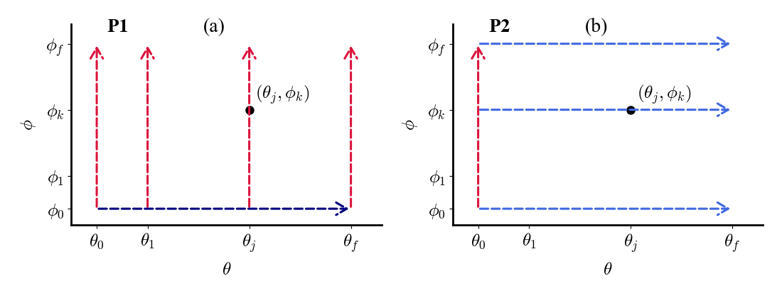
In this process of construction, we consider two distinct rectangular integration paths, denoted as P1 and P2. In path P1, the differential equations are first solved along the $\theta$ grid with a positive increment from $\theta=0^{\circ}$ to $90^{\circ}$ at a fixed $\phi=0^{\circ}$. Subsequently, for each $\theta$ value, integration is carried out along the $\phi$ grid from $\phi=0^{\circ}$ to $360^{\circ}$. In contrast, path P2 begins by integrating along the $\phi$ grid from $\phi=0^{\circ}$ to $360^{\circ}$ at fixed $\theta=0^{\circ}$ and then, continues along the $\theta$ grid for each $\phi$ value from $\theta=0^{\circ}$ to $90^{\circ}$. These integration schemes are illustrated in Figure S1 of the section S5 in SM. These two paths lead to different solutions of the ADT equations, resulting in path-dependent diabatic PES matrices. However, such matrices are related by another orthogonal matrix, ^{52, 21, 71} ensuring that all physical observables derived from them remain invariant ⁵⁴. Since path P1 facilitates the identification of closed contours, it is particularly convenient for locating CIs. On the other hand, to achieve greater numerical accuracy and to exploit the underlying symmetry of the system, path P2 is employed for constructing the diabatic PES matrices only upto $\phi$ = 120^∘ for each grid of $\rho$-$\theta$ space and thereby, can reduce the numerical effort (computational cost) by one third.

CONCLUSION

The “accuracy” of the molecular parameters as well as adiabatic PESs is one of the most important aspect for constructing the diabatic Hamiltonian. On the other hand, the location of CIs as well as the “accuracy” of associated NACTs are equally important, if not more, to determine the lifetime of the species from the excited electronic states. Moreover, the kinetic process for this chemical reaction will depend on the “accurate” adiabatic PESs as well as NACTs for different/between electronic states.

While exploring the details on the process of constructing diabatic Hamiltonian, it is important to follow the mechanism of the chemical reaction from the BBO perspective of structural (electronic) aspects of O₃: (a) location and nature of symmetry driven and accidental Jahn-Teller CIs to understand radiationless energy transfer; (b) the “accuracy” of non-adiabatic coupling elements through quantization of NACTs and their topological implications on the reaction attributes; (c) existence of SHS by examining the validaty of Curl Condition for low energy collision process, which varies from one reactive process to another; (d) construction of multi-state diabatic Hamiltonian matrix, which is, at present, four (N = 4) for O₃ case. Once such diabatic Hamiltonians are constructed involving even with singularities of NACTs, reaction attributes will be calculated and compared with experimental data as well as other theoretical results.

In this work, we present lowest four singlet adiabatic PESs ($\tilde{X}^{1}A^{\prime}$, $1^{1}A^{\prime\prime}$, $1^{1}A^{\prime}$ and $2^{1}A^{\prime\prime}$) of ozone as functions of Jacobi coordinates {$r$, $R$} for $\gamma$ = 0^∘, 45^∘ and 90^∘, computed using 7S-SA-MCSCF method followed by ic-MRCI(Q) with a full valence CAS(18e,12o) and AVQZ basis set, where the geometries and energetics at C_2v and D_3h configurations as well as the O₂ + O channel and high energy O + O + O asymptote are depicted with emphasis. Convergence of geometrical parameters, energetics and locations of minimum energy separation are also described with increasing basis set size. The NACTs are calculated employing 7S-SA-MCSCF method followed by CP-MCSCF approach along carefully chosen circular contours. A symmetry-driven CI involving the 2-3 electronic states at the D_3h geometry is characterized, along with the accidental C_2v and C_s ones between all the adjacent states (1-2, 2-3 and 3-4). The quantization of NACTs along the circular contours confirms the presence of CIs. Finally, for the purpose of future reactive scattering calculations on O₃ system and its isotopic variants, the adiabatic PESs [ic-MRCI(Q)], NACTs (CP-MCSCF), and the diabatic PES matrix are constructed using the same active space and basis set over the $\theta$–$\phi$ space at a specific $\rho$ (= 4 Bohr), which is a 2D cross section of the global 3D surface ($\rho$, $\theta$, $\phi$). Although the current model primarily includes low-lying singlet states, we have also investigated the effect of higher spin multiplicities by incorporating three triplet and three quintet states along with three singlets in the SA-MCSCF calculations. However, this extended state-averaging does not yield any improvement in the accuracy of the adiabatic PES compared to the singlet-only approach.

In our future study, we aim to explicitly incorporate SO interactions, which are crucial for capturing intersystem crossing effects and achieving a more complete representation of the nonadiabatic dynamics of ozone. Overall, the methodologies and insights presented in this study lay a basic foundation for the construction of global diabatic PES matrix for the application of BBO based scattering dynamics in ozone.

SUPPLEMENTARY MATERIAL

See the SM for explicit expressions of state specific ADT equations, diabatic potential matrix elements, path dependence of diabatic PES matrices, loation of CIs, curl condition and additional figures on adiabatic PESs.

AUTHOR DECLARATIONS

Conflict of Interest

The authors have no conflicts to disclose

DATA AVAILABILITY

The data that supports the findings of this study are available within the article and its supplementary material.

Supplementary Material

S1 Progresses on Adiabatic Potential Energy Surfaces of Ozone

In the early 1980s, the first computational work ⁹² on ozone was focused on its electronic structure and potential energy surfaces (PES). An analytical PES functions¹⁶ of ozone was derived by Varandas et. al. for the ground state by minimizing differences between observed and variationally calculated vibrational spectra, yielding accurate equilibrium force fields on which quasiclassical trajectory (QCT) calculation⁸⁵ had beed carried out. Later, using the Double Many-Body Expansion (DMBE), a simple and globally valid analytical PES for O₃ was developed⁸⁶ by fitting with experimental scattering and dissociation data. Rama Krishna et al. ⁴⁴ explored the dissociation energy of ozone using methods like Configuration Interaction and multi-configurational self-consistent field (MCSCF). This investigation highlighted the critical role of electronic correlation and paved the way for more refined models on the complex electronic and nuclear interactions of ozone. In 1991, Xantheas et al.⁹³ carried out full valence space MCSCF calculations on O₃ and revealed its critical features in ground-state adiabatic PES, including open and ring minima, and symmetry driven intersection seams. Yamashita et al. ⁹⁵ designed the initial wave packets for UV photodissociation studies rather than exploring dissociation in the ground electronic state. Subsequently, in trajectory calculations, the PES was empirically modified to remove the relatively high dissociation barrier. In 1997, Woywod et al.³¹ constructed the three low-lying 1 ¹A^′, 1 ¹A^′′ and 2 ¹A^′′ states of ozone and the corresponding transition-dipole-moment surfaces using CASSCF and CASPT2 methods, which are relevant for calculating Chappuis band. Their work also highlighted the importance of the ¹A^′′ - 2 ¹A^′′ conical intersection in ozone photodissociation dynamics. Other studies, including those by Banichevich et al. ¹² and Borowski et al. ¹⁵, provided partial PESs, while Xie et al. ⁹⁴ presented an accurate PES for near-equilibrium geometries. Tyuterev et al. ⁸¹ developed an effective ground-state potential energy function for ozone in the vicinity of the C_2v equilibrium configuration by least-squares fitting of extensive high-resolution experimental spectroscopic data. The potential was subsequently refined using an exact kinetic energy operator⁸², achieving near-spectroscopic accuracy for both vibrational and rotational energy levels and exhibiting physically correct long-range behavior. Later on, Banichevich et al. ¹² explored PESs for ground and excited states of ozone using MRCI methods to study dissociation pathways and photodissociation processes. Based on this study, Atchity and Ruedenberg (1997)⁵ introduced global PESs for the lowest two ${}^{1}A^{\prime}$ states, offering critical insights into the dissociation dynamics of ozone. Though the electronic structure of low-lying states of ozone were investigated by numerous researchers, only a couple of global PES for ozone were attempted using ab initio methods over limited region^{95, 78}.

S2 Strategy of ab initio calculations for adiabatic PESs and NACTs of Ozone (O₃)

Since we intend to develop multi-surface global diabatic Hamiltonian to explore the effect of electron-nuclear coupling through conical intersections between the surfaces on reactive cross-section and rate constant, it appears to be a necessity to calculate adiabatic potential energy surfaces as well as non-adiabatic coupling terms at the highest possible level of “accuracy” in ab initio calculation with the following motivation:

• All molecular as well as geometric parameters are in closest agreement with the latest experimental as well as other ab initio calculation(s).

• Locations and energetics of symmetry-driven as well as accidental degeneracies are reproduced within numerical “accuracy”, if such informations are available by other theoretical calculations.

• The quantization of ab initio calculated NACTs encapsulating $n\ (=1,2,...)$ number of conical intersections is verified by the magnitude, $n\pi$ (Jahn-Teller), $n.2\pi$ (Renner-Teller) and $0$ (Psedo Jahn-Teller)

• The existence of sub-Hilbert space through the equality of mathematical ($Z_{\theta\phi}^{ij}$) and ADT ($C_{\theta\phi}^{ij}$) curl using ab initio calculated NACTs over the entire configuration space.

Once the ab initio adiabatic PESs and NACTs are available over the entire configuration space and those quantities satisfy the above conditions within numerical “accuracy”, we construct the global diabatic Hamiltonian for scattering calculation to obtain cross-section and rate constants. As for examples, we have constructed so far the following diabatic surfaces of triatomic species and perform reaction dynamics:

• F+H₂: CAS(9e,10o), basis set: aug-cc-pVQZ, method: three state MRCI+Q

  Ref: J. Chem. Phys. 153, 174301, 2021; J. Phys. Chem. A 128 (8) 1438–1456, 2024

• H${}_{3}^{+}$: CAS(2e,10o), basis set: cc-pV5Z, method: three state MRCI

  Ref: J. Chem. Phys. 141, 204306, 2014; J. Chem. Phys. 147 (7), 074105, 2017; Phys. Chem. A 125, (3) 731–74, 2021

• HeH${}_{2}^{+}$: CAS(3e,8o), basis set: aug-cc-pVQZ, method: four state ic-MRCI

  Ref:J. Phys. Chem. A 127, 3832, 2023; J. Phys. Chem. A 128 (8), 1438–1456, 2024

• H₃: CAS(3e,16o), basis set: aug-cc-pVQZ, method: three state MRCI

  Ref:J. Phys. Chem. A 129, 6312, 2025

The associated diabatic Hamiltonians [in hyperspherical coordinates ($\rho$, $\theta$ and $\phi$) inter-convertible to Jacobi coordinates ($r,R$ and $\gamma$)] are published as subroutine (see the references above). In all the cases, the fitting of the diabatic matrix elements are avoided using general analytic functions rather locally fitted numerically for all required geometries in the dynamical calculation to attain higher accuracy. Since the fitting functions for ADT angles (or diabatic couplings) are not well known or even not an established procedure yet, we calculate astronomically large number of ab initio points to get accurate local fitting in all the above cases. Moreover, calculated cross section and rate constants using those diabatic surfaces for all the above systems show closest agreement with experimentally ones in comparison with results obtained from other existing diabatic PESs (see the above references on scattering calculations). Actually, the inclusion of NACTs in the construction of multi-state diabatic Hamiltonian is the single most important quantity after the “accuracy” of the adiabatic PESs to reproduce experimental data through scattering calculation.

Like the other systems (F+H₂, H${}_{3}^{+}$, HeH${}_{2}^{+}$ and H₃), in case of ozone (O₃), we are supposed to carry out nearly 1.5 million ab initio calculations at the ic-MRCI(Q) level for the low-lying four singlet adiabatic PESs and nearly two million ab initio points for NACT calculations as functions of hyperspherical coordiates ($2\leq\rho\leq 20$ Bohr, $0\leq\theta\leq\pi/2$, $0\leq\phi\leq 2\pi$). Indeed, we get the advantage of inherent symmetry of the species (O₃) that reduces the actual number of ab initio calculations. The other important aspect is the choice of the CAS(18e,12o) rather than the CAS(24e,15o). Although the latter [CAS(24e,15o)] can improves the dissociation energy of B1 [O₃ $\rightarrow$ O₂ + O] process, but it overestimates the dissociation energy of B2 process [O₂ $\rightarrow$ 2O]. On the other hand, the calculation of the global adiabatic and NACTs [followed by the construction of diabatic PES matrix] with the choice of CAS(24e,15o) at the ic-MRCI(Q) level could be virtually impossible due to the computational cost (see Table S1). Therefore, the following choice on methods and CAS/basis for calculating adiabatic PESs and NACTs at each ab initio point:

• Adiabatic PESs: Using CAS(18e,12o) and aug-cc-pVQZ basis, State Average MCSCF including seven low-lying singlet states for variational convergence followed by ic-MRCI incorporating Davidson correction to obtain the lowest four global adiabatic PESs.

• NACTs: Using CAS(18e,12o) and aug-cc-pVQZ basis, State Average MCSCF including seven low-lying singlet states for variational convergence followed by CP-MCSCF to calculate fifty four (54) nuclear gradients between the lowest four adiabatic PESs.

is the optimal one for reaching reasonable “accuracy” of the molecular parameters as well as for different processes (B1, B2, ..) and the coupling among the electronic states. Since our purpose is to construct the four state diabatic PES matrix and thereafter, to calculate cross section/rate constant for comparison with experimental results, the present level of calculation is itself a humongous task that could be recognized. Incidently, for the entire configuration space ($2\leq\rho\leq 20$ Bohr, $0\leq\theta\leq\pi/2$, $0\leq\phi\leq 2\pi$), calculations for the four (4) adiabatic PESs and six (6) NACTs at the 7S-SA-MCSCF and CP-MCSCF level, respectively, are already performed, but the ic-MRCI(Q) calculation for those adiabatic PESs are going on.

Table S1: Average computational time (in hours) and scratch memory usage (in GB) at the ic-MRCI(Q) level in the vicinity of different geometries of O₃ using CAS(18e,12o) and CAS(24e,15o) with increasing basis set size (AVQZ $\rightarrow$ AV6Z).

Geometry	CAS(18e,12o)			CAS(24e,15o)
	AVQZ	AV5Z	AV6Z	AVQZ	AV5Z	AV6Z
	Time (hours)
C2v minimum	10.8	19.8	37.0	38.2	80.8	118.9
D3h minimum	8.2	11.3	38.9	41.2	80.4	115.2
O2 + O channel	10.4	13.0	30.9	21.4	38.4	133.0
O + O + O asymptote	8.3	16.7	20.2	18.9	36.2	106.1
	Memory (GB)
C2v minimum	9.2	18.1	35.6	29.9	55.0	95.9
D3h minimum	8.6	18.1	35.6	29.9	55.0	95.9
O2 + O channel	8.6	18.0	35.4	29.8	55.0	95.8
O + O + O asymptote	8.5	18.1	35.4	29.8	55.0	95.7

S3 Adiabatic to Diabatic Transformation (ADT) equations for four (4) electronic state Sub-Hilbert space

In case of four (4) electronic state sub-Hilbert space, six (6) elementary rotation matrices can be multiplied in 6! ways to obtain the model ADT matrix where numerical solutions of any set of ADT equations originating from different permutation of elementary rotation matrix appear to be same. ⁶³ In the present work, the following permutation is adapted:

A $$= \textbf{A}^{12}(\Theta_{12}).\textbf{A}^{13}(\Theta_{13}).\textbf{A}^{23}(\Theta_{23}).\textbf{A}^{14}(\Theta_{14}).\textbf{A}^{24}(\Theta_{24}).\textbf{A}^{34}(\Theta_{34}),$$

where $\Theta$s are the ADT angles. The ADT equations are as follows:

$$\vec{\nabla}\Theta_{12} = -\vec{\tau}_{12}-\sin\Theta_{12}\tan\Theta_{13}\vec{\tau}_{13}-\cos\Theta_{12}\tan\Theta_{13}\vec{\tau}_{23}-\sin\Theta_{12}\sec\Theta_{13}\tan\Theta_{14}\vec{\tau}_{14}$$ (S1a)

$$-\cos\Theta_{12}\sec\Theta_{13}\tan\Theta_{14}\vec{\tau}_{24}$$

$$\vec{\nabla}\Theta_{13} = -\cos\Theta_{12}\vec{\tau}_{13}+\sin\Theta_{12}\vec{\tau}_{23}-\cos\Theta_{12}\sin\Theta_{13}\tan\Theta_{14}\vec{\tau}_{14}+\sin\Theta_{12}\sin\Theta_{13}\tan\Theta_{14}\vec{\tau}_{24}$$ (S1b)

$$-\cos\Theta_{13}\tan\Theta_{14}\vec{\tau}_{34}$$

$$\vec{\nabla}\Theta_{23} = -\cos\Theta_{13}[\vec{\tau}_{13}\sin\Theta_{12}\sec^{2}\Theta_{13}+\cos\Theta_{23}\sec\Theta_{14}(\vec{\tau}_{34}-\vec{\tau}_{24}\sin\Theta_{12}\tan\Theta_{13})\tan\Theta_{24}$$ (S1c)

$$+\sin\Theta_{12}\sec\Theta_{13}\tan\Theta_{13}\vec{\tau}_{14}\tan\Theta_{14}+\sin\Theta_{23}\vec{\tau}_{14}\sec\Theta_{14}\tan\Theta_{24}$$

$$+\cos\Theta_{12}\{\vec{\tau}_{23}\sec^{2}\Theta_{13}+\tan\Theta_{13}\cos\Theta_{23}\vec{\tau}_{14}\sec\Theta_{14}\tan\Theta_{24}+\sec\Theta_{13}(\tan\Theta_{13}\vec{\tau}_{24}\tan\Theta_{14}$$

$$+\sin\Theta_{23}\vec{\tau}_{24}\sec\Theta_{14}\tan\Theta_{24})\}]$$

$$\vec{\nabla}\Theta_{14} = -\cos\Theta_{12}\cos\Theta_{13}\vec{\tau}_{14}+\sin\Theta_{12}\cos\Theta_{13}\vec{\tau}_{24}+\sin\Theta_{13}\vec{\tau}_{34}$$ (S1d)

$$\vec{\nabla}\Theta_{24} = \sin\Theta_{23}(-\sin\Theta_{12}\sin\Theta_{13}\vec{\tau}_{24}\sec\Theta_{14}+\cos\Theta_{13}\vec{\tau}_{34}\sec\Theta_{14})-\sin\Theta_{12}\cos\Theta_{23}\vec{\tau}_{14}\sec\Theta_{14}$$ (S1e)

$$+\cos\Theta_{12}(\sin\Theta_{13}\sin\Theta_{23}\vec{\tau}_{14}\sec\Theta_{14}-\cos\Theta_{23}\vec{\tau}_{24}\sec\Theta_{14})$$

$$\vec{\nabla}\Theta_{34} = \sin\Theta_{12}\{-\sin\Theta_{23}\vec{\tau}_{14}\sec\Theta_{14}\sec\Theta_{24}+\sin\Theta_{13}\cos\Theta_{23}\vec{\tau}_{24}\sec\Theta_{14}\sec\Theta_{24}\}$$ (S1f)

$$+\cos\Theta_{12}[-\sec\Theta_{24}\{\sin\Theta_{13}\cos\Theta_{23}\vec{\tau}_{14}\sec\Theta_{14}+\sin\Theta_{23}\vec{\tau}_{24}\sec\Theta_{14}\}]$$

$$-\cos\Theta_{13}\cos\Theta_{23}\vec{\tau}_{34}\sec\Theta_{14}\sec\Theta_{24}$$

S4 Diabatic potential matrix elements for four (4) electronic state Sub-Hilbert space

$$W_{11} = u_{1}\cos^{2}{(\Theta_{12})}\cos^{2}{(\Theta_{13})}\cos^{2}{(\Theta_{14})}+u_{2}\sin^{2}{(\Theta_{12})}\cos^{2}{(\Theta_{13})}\cos^{2}{(\Theta_{14})}$$ (S2a)

$$+u_{3}\sin^{2}{(\Theta_{13})}\cos^{2}{(\Theta_{14})}+u_{4}\sin^{2}{(\Theta_{14})}$$

$$W_{22} = u_{1}[\{\sin{(\Theta_{12})}\cos{(\Theta_{23})}-\sin{(\Theta_{13})}\sin{(\Theta_{23})}\cos{(\Theta_{12})}\}\cos{(\Theta_{24})}-\sin{(\Theta_{14})}\sin{(\Theta_{24})}\cos{(\Theta_{12})}\cos{(\Theta_{13})}]^{2}$$ (S2b)

$$+u_{2}[\{\sin{(\Theta_{12})}\sin{(\Theta_{13})}\sin{(\Theta_{23})}+\cos{(\Theta_{12})}\cos{(\Theta_{23})}\}\cos{(\Theta_{24})}+\sin{(\Theta_{12})}\sin{(\Theta_{14})}\sin{(\Theta_{24})}\cos{(\Theta_{13})}]^{2}$$

$$+u_{3}\{\sin{(\Theta_{13})}\sin{(\Theta_{14})}\sin{(\Theta_{24})}-\sin{(\Theta_{23})}\cos{(\Theta_{13})}\cos{(\Theta_{24})}\}^{2}$$

$$+u_{4}\sin^{2}{(\Theta_{24})}\cos^{2}{(\Theta_{14})}$$

$$W_{33} = u_{1}\big[-[\{\sin{(\Theta_{12})}\cos{(\Theta_{23})}-\sin{(\Theta_{13})}\sin{(\Theta_{23})}\cos{(\Theta_{12})}\}\sin{(\Theta_{24})}$$ (S2c)

$$+\sin{(\Theta_{14})}\cos{(\Theta_{12})}\cos{(\Theta_{13})}\cos{(\Theta_{24})}]\sin{(\Theta_{34})}$$

$$+(\sin{(\Theta_{12})}\sin{(\Theta_{23})}+\sin{(\Theta_{13})}\cos{(\Theta_{12})}\cos{(\Theta_{23})})\cos{(\Theta_{34})}\big]^{2}$$

$$+u_{2}\big[-[\{\sin{(\Theta_{12})}\sin{(\Theta_{13})}\sin{(\Theta_{23})}+\cos{(\Theta_{12})}\cos{(\Theta_{23})}\}\sin{(\Theta_{24})}$$

$$-\sin{(\Theta_{12})}\sin{(\Theta_{14})}\cos{(\Theta_{13})}\cos{(\Theta_{24})}]\sin{(\Theta_{34})}$$

$$+\{-\sin{(\Theta_{12})}\sin{(\Theta_{13})}\cos{(\Theta_{23})}+\sin{(\Theta_{23})}\cos{(\Theta_{12})}\}\cos{(\Theta_{34})}\big]^{2}$$

$$+u_{3}[-\{-\sin{(\Theta_{13})}\sin{(\Theta_{14})}\cos{(\Theta_{24})}-\sin{(\Theta_{23})}\sin{(\Theta_{24})}\cos{(\Theta_{13})}\}\sin{(\Theta_{34})}$$

$$+\cos{(\Theta_{13})}\cos{(\Theta_{23})}\cos{(\Theta_{34})}]^{2}+u_{4}\sin^{2}{(\Theta_{34})}\cos^{2}{(\Theta_{14})}\cos^{2}{(\Theta_{24})}$$

$$W_{44} = u_{1}\big[[\{\sin{(\Theta_{12})}\cos{(\Theta_{23})}-\sin{(\Theta_{13})}\sin{(\Theta_{23})}\cos{(\Theta_{12})}\}\sin{(\Theta_{24})}$$ (S2d)

$$+\sin{(\Theta_{14})}\cos{(\Theta_{12})}\cos{(\Theta_{13})}\cos{(\Theta_{24})}]\cos{(\Theta_{34})}$$

$$+(\sin{(\Theta_{12})}\sin{(\Theta_{23})}+\sin{(\Theta_{13})}\cos{(\Theta_{12})}\cos{(\Theta_{23})})\sin{(\Theta_{34})}\big]^{2}+u_{2}\big[[\{\sin{(\Theta_{12})}\sin{(\Theta_{13})}\sin{(\Theta_{23})}$$

$$+\cos{(\Theta_{12})}\cos{(\Theta_{23})}\}\sin{(\Theta_{24})}-\sin{(\Theta_{12})}\sin{(\Theta_{14})}\cos{(\Theta_{13})}\cos{(\Theta_{24})}]\cos{(\Theta_{34})}$$

$$+(-\sin{(\Theta_{12})}\sin{(\Theta_{13})}\cos{(\Theta_{23})}+\sin{(\Theta_{23})}\cos{(\Theta_{12})})\sin{(\Theta_{34})}\big]^{2}+u_{3}[\{-\sin{(\Theta_{13})}\sin{(\Theta_{14})}\cos{(\Theta_{24})}$$

$$-\sin{(\Theta_{23})}\sin{(\Theta_{24})}\cos{(\Theta_{13})}\}\cos{(\Theta_{34})}+\sin{(\Theta_{34})}\cos{(\Theta_{13})}\cos{(\Theta_{23})}]^{2}$$

$$+u_{4}\cos^{2}{(\Theta_{14})}\cos^{2}{(\Theta_{24})}\cos^{2}{(\Theta_{34})}$$

$$W_{12} = u_{1}[\{\sin{(\Theta_{12})}\cos{(\Theta_{23})}-\sin{(\Theta_{13})}\sin{(\Theta_{23})}\cos{(\Theta_{12})}\}\cos{(\Theta_{24})}$$ (S3a)

$$-\sin{(\Theta_{14})}\sin{(\Theta_{24})}\cos{(\Theta_{12})}\cos{(\Theta_{13})}]\cos{(\Theta_{12})}\cos{(\Theta_{13})}\cos{(\Theta_{14})}$$

$$-u_{2}[\{\sin{(\Theta_{12})}\sin{(\Theta_{13})}\sin{(\Theta_{23})}+\cos{(\Theta_{12})}\cos{(\Theta_{23})}\}\cos{(\Theta_{24})}$$

$$+\sin{(\Theta_{12})}\sin{(\Theta_{14})}\sin{(\Theta_{24})}\cos{(\Theta_{13})}]\sin{(\Theta_{12})}\cos{(\Theta_{13})}\cos{(\Theta_{14})}-u_{3}\{\sin{(\Theta_{13})}\sin{(\Theta_{14})}\sin{(\Theta_{24})}$$

$$-\sin{(\Theta_{23})}\cos{(\Theta_{13})}\cos{(\Theta_{24})}\}\sin{(\Theta_{13})}\cos{(\Theta_{14})}+u_{4}\sin{(\Theta_{14})}\sin{(\Theta_{24})}\cos{(\Theta_{14})}$$

$$W_{13} = u_{1}\big[-[\{\sin{(\Theta_{12})}\cos{(\Theta_{23})}-\sin{(\Theta_{13})}\sin{(\Theta_{23})}\cos{(\Theta_{12})}\}\sin{(\Theta_{24})}$$ (S3b)

$$+\sin{(\Theta_{14})}\cos{(\Theta_{12})}\cos{(\Theta_{13})}\cos{(\Theta_{24})}]\sin{(\Theta_{34})}$$

$$+\{\sin{(\Theta_{12})}\sin{(\Theta_{23})}+\sin{(\Theta_{13})}\cos{(\Theta_{12})}\cos{(\Theta_{23})}\}\cos{(\Theta_{34})}\big]\cos{(\Theta_{12})}\cos{(\Theta_{13})}\cos{(\Theta_{14})}$$

$$-u_{2}\big[-[\{\sin{(\Theta_{12})}\sin{(\Theta_{13})}\sin{(\Theta_{23})}+\cos{(\Theta_{12})}\cos{(\Theta_{23})}\}\sin{(\Theta_{24})}$$

$$-\sin{(\Theta_{12})}\sin{(\Theta_{14})}\cos{(\Theta_{13})}\cos{(\Theta_{24})}]\sin{(\Theta_{34})}+\{-\sin{(\Theta_{12})}\sin{(\Theta_{13})}\cos{(\Theta_{23})}$$

$$+\sin{(\Theta_{23})}\cos{(\Theta_{12})}\}\cos{(\Theta_{34})}\big]\sin{(\Theta_{12})}\cos{(\Theta_{13})}\cos{(\Theta_{14})}$$

$$-u_{3}[-\{-\sin{(\Theta_{13})}\sin{(\Theta_{14})}\cos{(\Theta_{24})}-\sin{(\Theta_{23})}\sin{(\Theta_{24})}\cos{(\Theta_{13})}\}\sin{(\Theta_{34})}$$

$$+\cos{(\Theta_{13})}\cos{(\Theta_{23})}\cos{(\Theta_{34})}]\sin{(\Theta_{13})}\cos{(\Theta_{14})}$$

$$+u_{4}\sin{(\Theta_{14})}\sin{(\Theta_{34})}\cos{(\Theta_{14})}\cos{(\Theta_{24})}$$

$$W_{23} = u_{1}\big[-[\{\sin{(\Theta_{12})}\cos{(\Theta_{23})}-\sin{(\Theta_{13})}\sin{(\Theta_{23})}\cos{(\Theta_{12})}\}\sin{(\Theta_{24})}$$ (S4a)

$$+\sin{(\Theta_{14})}\cos{(\Theta_{12})}\cos{(\Theta_{13})}\cos{(\Theta_{24})}]\sin{(\Theta_{34})}$$

$$+\{\sin{(\Theta_{12})}\sin{(\Theta_{23})}+\sin{(\Theta_{13})}\cos{(\Theta_{12})}\cos{(\Theta_{23})}\}\cos{(\Theta_{34})}\big][\{\sin{(\Theta_{12})}\cos{(\Theta_{23})}$$

$$-\sin{(\Theta_{13})}\sin{(\Theta_{23})}\cos{(\Theta_{12})}\}\cos{(\Theta_{24})}-\sin{(\Theta_{14})}\sin{(\Theta_{24})}\cos{(\Theta_{12})}\cos{(\Theta_{13})}]$$

$$+u_{2}\big[-[\{\sin{(\Theta_{12})}\sin{(\Theta_{13})}\sin{(\Theta_{23})}+\cos{(\Theta_{12})}\cos{(\Theta_{23})}\}\sin{(\Theta_{24})}$$

$$-\sin{(\Theta_{12})}\sin{(\Theta_{14})}\cos{(\Theta_{13})}\cos{(\Theta_{24})}]\sin{(\Theta_{34})}+(-\sin{(\Theta_{12})}\sin{(\Theta_{13})}\cos{(\Theta_{23})}$$

$$+\sin{(\Theta_{23})}\cos{(\Theta_{12})})\cos{(\Theta_{34})}\big][\{\sin{(\Theta_{12})}\sin{(\Theta_{13})}\sin{(\Theta_{23})}+\cos{(\Theta_{12})}\cos{(\Theta_{23})}\}\cos{(\Theta_{24})}$$

$$+\sin{(\Theta_{12})}\sin{(\Theta_{14})}\sin{(\Theta_{24})}\cos{(\Theta_{13})}]$$

$$+u_{3}[-\{-\sin{(\Theta_{13})}\sin{(\Theta_{14})}\cos{(\Theta_{24})}-\sin{(\Theta_{23})}\sin{(\Theta_{24})}\cos{(\Theta_{13})}\}\sin{(\Theta_{34})}$$

$$+\cos{(\Theta_{13})}\cos{(\Theta_{23})}\cos{(\Theta_{34})}]\{\sin{(\Theta_{13})}\sin{(\Theta_{14})}\sin{(\Theta_{24})}-\sin{(\Theta_{23})}\cos{(\Theta_{13})}\cos{(\Theta_{24})}\}$$

$$+u_{4}\sin{(\Theta_{24})}\sin{(\Theta_{34})}\cos^{2}{(\Theta_{14})}\cos{(\Theta_{24})}$$

$$W_{14} = u_{1}\big[[\{\sin{(\Theta_{12})}\cos{(\Theta_{23})}-\sin{(\Theta_{13})}\sin{(\Theta_{23})}\cos{(\Theta_{12})}\}\sin{(\Theta_{24})}$$ (S4b)

$$+\sin{(\Theta_{14})}\cos{(\Theta_{12})}\cos{(\Theta_{13})}\cos{(\Theta_{24})}]\cos{(\Theta_{34})}+\{\sin{(\Theta_{12})}\sin{(\Theta_{23})}$$

$$+\sin{(\Theta_{13})}\cos{(\Theta_{12})}\cos{(\Theta_{23})}\}\sin{(\Theta_{34})}\big]\cos{(\Theta_{12})}\cos{(\Theta_{13})}\cos{(\Theta_{14})}$$

$$-u_{2}\big[[\{\sin{(\Theta_{12})}\sin{(\Theta_{13})}\sin{(\Theta_{23})}+\cos{(\Theta_{12})}\cos{(\Theta_{23})}\}\sin{(\Theta_{24})}$$

$$-\sin{(\Theta_{12})}\sin{(\Theta_{14})}\cos{(\Theta_{13})}\cos{(\Theta_{24})}]\cos{(\Theta_{34})}+\{-\sin{(\Theta_{12})}\sin{(\Theta_{13})}\cos{(\Theta_{23})}$$

$$+\sin{(\Theta_{23})}\cos{(\Theta_{12})}\}\sin{(\Theta_{34})}\big]\sin{(\Theta_{12})}\cos{(\Theta_{13})}\cos{(\Theta_{14})}-u_{3}[\{-\sin{(\Theta_{13})}\sin{(\Theta_{14})}\cos{(\Theta_{24})}$$

$$-\sin{(\Theta_{23})}\sin{(\Theta_{24})}\cos{(\Theta_{13})}\}\cos{(\Theta_{34})}+\sin{(\Theta_{34})}\cos{(\Theta_{13})}\cos{(\Theta_{23})}]\sin{(\Theta_{13})}\cos{(\Theta_{14})}$$

$$-u_{4}\sin{(\Theta_{14})}\cos{(\Theta_{14})}\cos{(\Theta_{24})}\cos{(\Theta_{34})}$$

$$W_{24} = u_{1}\big[[\{\sin{(\Theta_{12})}\cos{(\Theta_{23})}-\sin{(\Theta_{13})}\sin{(\Theta_{23})}\cos{(\Theta_{12})}\}\sin{(\Theta_{24})}$$ (S5a)

$$+\sin{(\Theta_{14})}\cos{(\Theta_{12})}\cos{(\Theta_{13})}\cos{(\Theta_{24})}]\cos{(\Theta_{34})}+\{\sin{(\Theta_{12})}\sin{(\Theta_{23})}$$

$$+\sin{(\Theta_{13})}\cos{(\Theta_{12})}\cos{(\Theta_{23})}\}\sin{(\Theta_{34})}\big][\{\sin{(\Theta_{12})}\cos{(\Theta_{23})}-\sin{(\Theta_{13})}\sin{(\Theta_{23})}\cos{(\Theta_{12})}\}\cos{(\Theta_{24})}$$

$$-\sin{(\Theta_{14})}\sin{(\Theta_{24})}\cos{(\Theta_{12})}\cos{(\Theta_{13})}]+u_{2}\big[[\{\sin{(\Theta_{12})}\sin{(\Theta_{13})}\sin{(\Theta_{23})}+\cos{(\Theta_{12})}\cos{(\Theta_{23})}\}\sin{(\Theta_{24})}$$

$$-\sin{(\Theta_{12})}\sin{(\Theta_{14})}\cos{(\Theta_{13})}\cos{(\Theta_{24})}]\cos{(\Theta_{34})}+\{-\sin{(\Theta_{12})}\sin{(\Theta_{13})}\cos{(\Theta_{23})}$$

$$+\sin{(\Theta_{23})}\cos{(\Theta_{12})}\}\sin{(\Theta_{34})}\big][\{\sin{(\Theta_{12})}\sin{(\Theta_{13})}\sin{(\Theta_{23})}+\cos{(\Theta_{12})}\cos{(\Theta_{23})}\}\cos{(\Theta_{24})}$$

$$+\sin{(\Theta_{12})}\sin{(\Theta_{14})}\sin{(\Theta_{24})}\cos{(\Theta_{13})}]$$

$$+u_{3}[\{-\sin{(\Theta_{13})}\sin{(\Theta_{14})}\cos{(\Theta_{24})}-\sin{(\Theta_{23})}\sin{(\Theta_{24})}\cos{(\Theta_{13})}\}\cos{(\Theta_{34})}$$

$$+\sin{(\Theta_{34})}\cos{(\Theta_{13})}\cos{(\Theta_{23})}]\{\sin{(\Theta_{13})}\sin{(\Theta_{14})}\sin{(\Theta_{24})}$$

$$-\sin{(\Theta_{23})}\cos{(\Theta_{13})}\cos{(\Theta_{24})}\}-u_{4}\sin{(\Theta_{24})}\cos^{2}{(\Theta_{14})}\cos{(\Theta_{24})}\cos{(\Theta_{34})}$$

$$W_{34} = u_{1}\big[-[\{\sin{(\Theta_{12})}\cos{(\Theta_{23})}-\sin{(\Theta_{13})}\sin{(\Theta_{23})}\cos{(\Theta_{12})}\}\sin{(\Theta_{24})}$$ (S5b)

$$+\sin{(\Theta_{14})}\cos{(\Theta_{12})}\cos{(\Theta_{13})}\cos{(\Theta_{24})}]\sin{(\Theta_{34})}$$

$$+\{\sin{(\Theta_{12})}\sin{(\Theta_{23})}+\sin{(\Theta_{13})}\cos{(\Theta_{12})}\cos{(\Theta_{23})}\}\cos{(\Theta_{34})}\big]\big[[\{\sin{(\Theta_{12})}\cos{(\Theta_{23})}$$

$$-\sin{(\Theta_{13})}\sin{(\Theta_{23})}\cos{(\Theta_{12})}\}\sin{(\Theta_{24})}+\sin{(\Theta_{14})}\cos{(\Theta_{12})}\cos{(\Theta_{13})}\cos{(\Theta_{24})}]\cos{(\Theta_{34})}$$

$$+\{\sin{(\Theta_{12})}\sin{(\Theta_{23})}+\sin{(\Theta_{13})}\cos{(\Theta_{12})}\cos{(\Theta_{23})}\}\sin{(\Theta_{34})}\big]+u_{2}\big[-[\{\sin{(\Theta_{12})}\sin{(\Theta_{13})}\sin{(\Theta_{23})}$$

$$+\cos{(\Theta_{12})}\cos{(\Theta_{23})}\}\sin{(\Theta_{24})}-\sin{(\Theta_{12})}\sin{(\Theta_{14})}\cos{(\Theta_{13})}\cos{(\Theta_{24})}]\sin{(\Theta_{34})}$$

$$+\{-\sin{(\Theta_{12})}\sin{(\Theta_{13})}\cos{(\Theta_{23})}+\sin{(\Theta_{23})}\cos{(\Theta_{12})}\}\cos{(\Theta_{34})}\big]\big[[\{\sin{(\Theta_{12})}\sin{(\Theta_{13})}\sin{(\Theta_{23})}$$

$$+\cos{(\Theta_{12})}\cos{(\Theta_{23})}\}\sin{(\Theta_{24})}-\sin{(\Theta_{12})}\sin{(\Theta_{14})}\cos{(\Theta_{13})}\cos{(\Theta_{24})}]\cos{(\Theta_{34})}$$

$$+\{-\sin{(\Theta_{12})}\sin{(\Theta_{13})}\cos{(\Theta_{23})}+\sin{(\Theta_{23})}\cos{(\Theta_{12})}\}\sin{(\Theta_{34})}\big]+u_{3}[-\{-\sin{(\Theta_{13})}\sin{(\Theta_{14})}\cos{(\Theta_{24})}$$

$$-\sin{(\Theta_{23})}\sin{(\Theta_{24})}\cos{(\Theta_{13})}\}\sin{(\Theta_{34})}+\cos{(\Theta_{13})}\cos{(\Theta_{23})}\cos{(\Theta_{34})}][\{-\sin{(\Theta_{13})}\sin{(\Theta_{14})}\cos{(\Theta_{24})}$$

$$-\sin{(\Theta_{23})}\sin{(\Theta_{24})}\cos{(\Theta_{13})}\}\cos{(\Theta_{34})}+\sin{(\Theta_{34})}\cos{(\Theta_{13})}\cos{(\Theta_{23})}]$$

$$-u_{4}\sin{(\Theta_{34})}\cos^{2}{(\Theta_{14})}\cos^{2}{(\Theta_{24})}\cos{(\Theta_{34})}$$

S5 Diabatic PES matrices constructed along different paths of integration

FIG. S1: The 2D rectangular paths along which the ADT equations are solved.

Let us choose two different 2D contour integration of ADT equations along $\theta$ and $\phi$ for a fixed $\rho$ as shown in Figures S1(a) and S1(b) and such ADT matrices are termed as $A_{1}$ and $A_{2}$, where those matrices are orthonormal by construction at any point in configuration space:

$$\mathbf{A_{1}{{}^{\dagger}}}(\theta,\phi)\,\mathbf{A_{1}}(\theta,\phi)=\mathbf{I}$$ (S6a)

$$\mathbf{A_{2}{{}^{\dagger}}}(\theta,\phi)\,\mathbf{A_{2}}(\theta,\phi)=\mathbf{I}$$ (S6b)

Furthermore, we consider the following product matrix:

$$\mathbf{B}(\theta,\phi)=\mathbf{A_{1}{{}^{\dagger}}}(\theta,\phi)\mathbf{A_{2}}(\theta,\phi),$$ (S7)

which also appears as an orthogonal matrix:

$$\mathbf{B{{}^{\dagger}}}\,\mathbf{B} = \left(\mathbf{A_{1}{{}^{\dagger}}}\,\mathbf{A_{2}}\right)^{\dagger}\,\left(\mathbf{A_{1}{{}^{\dagger}}}\,\mathbf{A_{2}}\right)$$ (S8)

$$= \mathbf{A_{2}{{}^{\dagger}}}\left(\mathbf{A_{1}}\,\mathbf{A_{1}{{}^{\dagger}}}\right)\,\mathbf{A_{2}}$$

$$= \mathbf{I}$$

From Equation S7, one can get the following relation:

$$\mathbf{A_{1}}\,\mathbf{B}=\mathbf{A_{2}},$$ (S9)

which indicates that the ADT matrices belonging to two different paths are related through another orthogonal matrix (B).

On the other hand, the diabatic PESs matrices along two different paths of integration takes the following form:

$$\mathbf{W_{1}} = \mathbf{A_{1}{{}^{\dagger}}}\mathbf{U}\mathbf{A_{1}}$$ (S10a)

$$\mathbf{W_{2}} = \mathbf{A_{2}{{}^{\dagger}}}\mathbf{U}\mathbf{A_{2}},\qquad\text{$\mathbf{U}$ is adiabatic PESs matrix (diagonal)}$$ (S10b)

which leads to

$$\mathbf{A_{1}}\,\mathbf{W_{1}}\,\mathbf{A_{1}{{}^{\dagger}}}=\mathbf{U}$$ (S11a)

$$\mathbf{A_{2}}\,\mathbf{W_{2}}\,\mathbf{A_{2}{{}^{\dagger}}}=\mathbf{U}$$ (S11b)

Comparing Equation S11(a) and S11(b), we obtain:

$$\mathbf{A_{1}}\,\mathbf{W_{1}}\,\mathbf{A_{1}{{}^{\dagger}}} = \mathbf{A_{2}}\,\mathbf{W_{2}}\,\mathbf{A_{2}{{}^{\dagger}}}$$

$$\mathbf{A_{1}{{}^{\dagger}}}\,\mathbf{A_{1}}\,\mathbf{W_{1}}\,\mathbf{A_{1}{{}^{\dagger}}}\,\mathbf{A_{1}} = \mathbf{A_{1}{{}^{\dagger}}}\,\mathbf{A_{2}}\,\mathbf{W_{2}}\,\mathbf{A_{2}{{}^{\dagger}}}\,\mathbf{A_{1}}$$

$$\mathbf{W_{1}} = \mathbf{B}\,\mathbf{W_{2}}\,\mathbf{B}^{\dagger}$$ (S12)

Therefore, the diabatic PESs matrices along two different paths are related through another orthogonal matrix (B) and thus, calculated observables should be path independent in theoretical consideration.

S6 7S-SA-MCSCF level Adiabatic PESs using CAS(18e,12o) and AVQZ basis

FIG. S2: Lowest four adiabatic PESs of O₃ at $\gamma=0^{\circ}$ using 7S-SA-MCSCF method with CAS(18e,12o) and the AVQZ basis set.

FIG. S3: Lowest four adiabatic PESs of O₃ at $\gamma=45^{\circ}$ using 7S-SA-MCSCF method with CAS(18e,12o) and the AVQZ basis set.

FIG. S4: Lowest four adiabatic PESs of O₃ at $\gamma=90^{\circ}$ using 7S-SA-MCSCF method with CAS(18e,12o) and the AVQZ basis set.

S7 Location of CIs

\begin{overpic}[width=607.06534pt]{r_3.06_D3h_23.pdf} \put(5.0,75.0){{(a)}} \end{overpic}

\begin{overpic}[width=607.06534pt]{r_4.1_C2v_23.pdf} \put(5.0,75.0){{(b)}} \end{overpic}

\begin{overpic}[width=607.06534pt]{r_3.85_C2v_1234.pdf} \put(0.0,70.0){{(c)}} \end{overpic}

FIG. S5: The adiabatic PECs at different $R$ as a function of $r$ at $\gamma$ = 90^∘ are depicted as function of $R$ for various values of $r$ to explore the location of C_2v and D_3h CIs.

S8 Curl Condition

FIG. S6: Mathematical curl ($Z_{\theta\phi}^{ij}$) and the ADT curl ($C_{\theta\phi}^{ij}$) as well as Curl Condition ($F_{\theta\phi}^{ij}$) are presented as a function of $\phi$ for fixed $\rho$ = 4 Bohr at different $\theta$, namely, 50^∘, 70^∘ and 90^∘