Probing the Dispersion and Rotation Measure Contributions from Supernova Remnants in Fast Radio Burst Source Environments with 1D SNR Simulation

Abstract

Fast radio bursts (FRBs) provide a sensitive probe of ionized baryons through their dispersion measure (DM). In addition to slowly evolving cosmological terms, at least two repeaters now show clear secular DM-decrease episodes: FRB 20190520B and FRB 20121102 (the latter with a two-stage trend: early mild rise and late decline), supporting a dense, dynamically evolving local environment. We adopt a forward-modeling approach and use time-dependent 1D SNR simulations for a young magnetar embedded in SN ejecta, combining single-star and binary-stripped progenitors with HD+NEI calculations to follow shock structure, ionization, and electron density. The shocked region contributes only limited DM ($\lesssim 10\,{\rm pc\,cm^{-3}}$), while the dominant time-varying component is the unshocked ejecta, whose early behavior follows ${\rm DM}\propto t^{-\alpha}$ with $\alpha\simeq 1.8$–$1.9$. Although shocked-region DM is small, shock-amplified magnetic fields can still generate substantial RM; in our shock-only RM framework, only the $11\,M_{\odot}$ SS model reproduces the FRB 20121102 RM evolution. Binary-stripped progenitors generally yield smaller DM than single-star models at fixed $M_{\rm ZAMS}$, with composition-dependent mean molecular weights introducing non-monotonic mass trends. Matching the observed ${\rm dDM}/{\rm d}t$ of FRB 20190520B (and the late-stage slope of FRB 20121102), we infer local SNR DM contributions of tens to hundreds ${\rm pc\,cm^{-3}}$. We also find GHz escape is allowed in most models, with $\tau_{\rm ff}=1$ typically reached by $t_{\rm esc}\lesssim 70$ yr; for weakly ionized ejecta, the source can be nearly transparent from very early times. These results support a young CCSN/SNR origin for a substantial fraction of ${\rm DM}_{\rm source}$ and highlight that physically consistent local-environment modeling is essential for robust FRB cosmological DM inferences.

show]kawashima@kusastro.kyoto-u.ac.jp

I Introduction

FRBs are short ($\sim$ms), bright radio transients with large dispersion measures (DMs), implying extragalactic or even cosmological distances. Since the first Lorimer burst (Lorimer2007), the DM budget of FRBs has been recognized as a key observable, connecting FRBs to the baryon content of the Universe (McQuinn2014; DZ2014; Zheng2014; Li2019...876...146; Macquart2020Nature; Simha2020; Takahashi2021MNRAS; Medlock2021; Zhu2021; Lee2022; KHRYKIN2024; Medlock2024; Connor2024; ZZ2025; Konietzka2025arXiv) as well as to the physical conditions in their local environments (see also the review by Zhan2023RvMP). Repeating FRBs with well-sampled monitoring campaigns now reveal that the DM is not constant over time; it can vary secularly on timescales of years, suggesting that at least part of the DM originates in a dynamical, evolving medium near the source.

A natural framework is that at least some FRBs are produced by young magnetars embedded in SNRs and their surrounding circumstellar medium (CSM). In this picture, the total observed FRB DM can be decomposed into several contributions:

$${\rm DM}_{\rm FRB}={\rm DM}_{\rm MW}+{\rm DM}_{\rm Halos}+{\rm DM}_{\rm IGM}+\frac{{\rm DM}_{\rm HG}+{\rm DM}_{\rm source}}{1+z},$$ (1)

Where ${\rm DM}_{\rm MW}$ is the contribution from the Milky Way, including both the interstellar medium (${\rm DM}_{\rm MW,ISM}$) and the Milky Way’s circumgalactic halo (${\rm DM}_{\rm MW,halo}$). ${\rm DM}_{\rm Halos}$ represents the cumulative contribution from all intervening galactic halos along the line of sight, i.e.,

$${\rm DM}_{\rm Halos}=\sum_{i}\frac{{\rm DM}_{\rm halo,i}}{1+z_{i}},$$

where each term corresponds to the circumgalactic medium (CGM) of a foreground galaxy intersected by the FRB sight line, ${\rm DM}_{\rm IGM}$ collects the contributions from the intergalactic medium, ${\rm DM}_{\rm HG}$ is the contribution from the host galaxy, and ${\rm DM}_{\rm source}$ is the local contribution in the immediate vicinity of the FRB engine (typically on parsec or sub-parsec scales). On timescales of $\sim$years, all components except ${\rm DM}_{\rm source}$ are expected to be negligible (Yang&Zhang2017), so any observed secular change in DM is naturally attributed to the evolution of the source environment. However, the ${\rm DM}_{\rm source}$ inferred from the observed DM-decay slope is itself model dependent; therefore, an apparent local DM excess can remain partially degenerate with ${\rm DM}_{\rm Halos}$ from foreground structures, leading to ongoing debate in some sources. FRB 20190520B provides a representative example, with a source-dominated interpretation (ZYZhao2021b) versus a substantial foreground-halo/cluster contribution (Lee2023).

Previous theoretical work (Yang2017ApJ...839L..25Y; Murase2016; Kashiyama2017; Yang&Zhang2017) has explored a variety of possible contributors to ${\rm DM}_{\rm source}$. These include (i) the SNR ejecta and shocked shell (e.g., Piro2016; Piro&Gaensler2018; Niu2025), (ii) a nebula powered by the relativistic pulsar/magnetar wind (e.g., Yang2016; Margalit2018; Metzger2019; ZYZhao2021b; Mahlmann2022), (iii) dense star-forming or H II regions in the host galaxy (e.g., Tendulkar2017; Michilli2018Natur; Bassa2017), and (iv) small-scale plasma lensing structures (e.g., Cordes2017; Main2018Natur). Among these, the SNR scenario is particularly attractive for sources with large host DM and significant negative $\mathrm{dDM}/\mathrm{d}t$, in which an expanding ionized shell naturally leads to a declining DM over time. Analytic models based on the McKee & Truelove treatment of SNR evolution have been used to estimate the time dependence of the SNR DM in different expansion phases—ejecta-dominated (ED), Sedov–Taylor (ST), and radiative snowplow—(McKee&Truelove1995PhR; McKee&Truelove1999; Piro2016; Piro&Gaensler2018), and to place constraints on the age and environment of individual FRB sources.

On the observational side, several FRBs show a substantial excess or variations in their DM or Rotation Measure (RM) (Masui2015Natur; Hilmarsson2021; Niu2022; Wang2022NatCo; Mckinven2023), indicating the presence of a dense and magnetized local environment. FRB 20190520B shows a clear long-term secular decrease in DM, with a nearly linear decline over $\sim 4$ years at ${\rm dDM}/{\rm d}t\simeq-12\,{\rm pc\,cm^{-3}\,yr^{-1}}$ (Niu2025). Recent monitoring of FRB 20121102 also reveals secular DM evolution, but with a two-stage behavior: an early segment with slight DM increase and a late segment with DM decrease (Wang2025arXiv250715790W). In this work, when performing SNR slope matching for FRB 20121102, we use the late (declining) segment. The slope turnover between the early and late stages may indicate additional local-plasma components (e.g., MWN-related contributions), consistent with hybrid interpretations discussed in Dai2017, Beloborodov2017, and Yang2019. We also note recent attempts to place active repeaters within a unified framework, including FRB 20190417A, an active repeater with periodic activity that shows oscillatory RM with sign reversals and is generally interpreted in a magnetar–massive-star binary environment, as well as persistent radio source (PRS)-associated systems (Wang2025arXiv251207140W).

Beyond these analytical estimates of the SNR contribution to ${\rm DM}_{\rm source}$, numerical simulations provide a natural and complementary approach for studying the dynamical evolution of SNRs and its imprint on FRB DM. Modern stellar evolution calculations, such as those performed with MESA (version 12115; Paxton2011ModulesMESA; Paxton2013ModulesStars; Paxton2015ModulesExplosions; Paxton2018ModulesExplosions; Paxton2019ModulesConservation; Jermyn2023ModulesInfrastructure), self-consistently follow massive stars from the zero-age main sequence (ZAMS) to core collapse (CC), thereby providing realistic progenitor structures and ejecta properties as inputs for subsequent CCSNR simulations.

At the same time, numerical simulations of supernova remnants have rapidly advanced, ranging from one-dimensional (1D) models that incorporate detailed shock physics, radiative cooling, non-equilibrium ionization (NEI), and cosmic ray (CR) acceleration (e.g., Patnaude2010; Lee+2012; Lee+2013; Lee+2014; Diesing2019; Diesing2024; Diesing2025) to multi-dimensional (2D/3D) simulations that reveal the importance of pulsar wind nebulae (PWN), hydrodynamic instabilities, ejecta clumping, asymmetric ejecta–CSM interactions (e.g., Blondin2001; Ferrand2010; Orlando2012; Ferrand2012; Ferrand2019).

While previous analytical studies have provided valuable insights into the global shock structure and approximate DM scalings, they often adopt simplified progenitor and CSM configurations. In particular, massive single stars and binary-stripped (BS) progenitors are expected to produce markedly different CSM density profiles due to their distinct mass-loss histories and wind properties (Patnaude2017; Jacovich+2021; Laplace+2021; Farmer+2023; KawashimaSubmitted). Such differences can lead to SNR density and ionization structures, and hence DM evolution, that deviate substantially from the idealized time-scaling relations commonly assumed in analytical models.

Motivated by these considerations, in this work we take a step beyond analytic scalings and investigate the contribution of SNR to ${\rm DM}_{\rm source}$ using detailed 1D HD simulations with NEI and radiative cooling. We aim to test whether, and under what conditions, self-consistent HD SNR models can reproduce the range of ${\rm DM}_{\rm source}$, $\mathrm{dDM}/\mathrm{d}t$, and ${\rm RM}_{\rm source}$ inferred from FRB observations. In particular, we investigate whether specific combinations of ZAMS mass, ejecta mass, and circumstellar density structure, as expected from single-star (SS) and BS progenitors, can satisfy the observational constraints on both the absolute DM and its time evolution.

This draft is organized as follows. In Section II, we briefly summarize different contributions to the FRB DM budget and motivate the focus on the local ${\rm DM}_{\rm source}$ term. Section IV presents the numerical methodology adopted in this work, including the CSM modeling, SNR simulation setup, and the calculation methods for DM, optical depth, and RM. Section V presents results for two cases $M_{\rm ZAMS}=11\,M_{\odot}$ and $M_{\rm ZAMS}=30\,M_{\odot}$, including the time evolution of DM, its derivatives, free-free optical depth, RM evolution and ${\rm RM}_{\rm source}$ constraints, comparisons with analytic/semi-analytic models, and shocked-region electron-source decomposition. We discuss model limitations and future directions in Section VI, and provide a summary in Section VII.

II FRB DM Components and Local Source Environment

II.1 Decomposition of the FRB DM budget

For a given FRB, the total observed DM can be written as in Eq. (1). For convenience, we define the non-local (large-scale, slowly varying) component,

$${\rm DM}_{\rm diff}\equiv{\rm DM}_{\rm IGM}+{\rm DM}_{\rm Halos},$$ (2)

$${\rm DM}_{\rm nonlocal}\equiv{\rm DM}_{\rm MW}+{\rm DM}_{\rm diff}+\frac{{\rm DM}_{\rm HG}}{1+z},$$ (3)

so that

$${\rm DM}_{\rm FRB}={\rm DM}_{\rm nonlocal}+\frac{{\rm DM}_{\rm source}}{1+z}.$$ (4)

Here ${\rm DM}_{\rm diff}$ traces large-scale structure along the line of sight and is the component that can be robustly estimated from cosmological simulations or empirical DM–$z$ relations. These non-local terms are expected to vary negligibly over human timescales. By contrast, ${\rm DM}_{\rm source}$ is associated with the local environment of the FRB engine, on scales from $\lesssim 0.1$ pc (PWN and magnetar wind nebula) to a few pc (SNR shell and surrounding H II region). Because this material can evolve dynamically on timescales of years–decades, ${\rm DM}_{\rm source}$ can in principle be responsible for the secular DM evolution seen in some repeating FRBs. Moreover, since ${\rm DM}_{\rm source}$ is sensitive to the progenitor history and explosion properties, it may carry information about whether the FRB source formed in a SS or BS channel.

In the following, we focus on modeling ${\rm DM}_{\rm source}$ originating in the SNR and its shocked surroundings. Other local contributors (PWN, H II regions, plasma lenses) will be briefly discussed in Section II.2 as complementary or additional components.

II.2 Candidate local environments: SNR, PWN, H II region, plasma lensing

Previous work has explored several possible local environments that could contribute significantly to the FRB DM and its time evolution:

• SNR: An expanding SNR ejecta and its forward shock shell provide a natural reservoir of dense ionized gas whose column density decreases over time. In previous FRB–SNR theoretical studies, the temporal evolution of the SNR has often been modeled using the self-similar solutions of McKee&Truelove1995PhR, which describes the ED, ST, and radiative snowplow phases. Within this analytic framework, the resulting DM evolution is commonly written as ${\rm DM}_{\rm SNR}\propto t^{-\alpha}$ with $0\lesssim\alpha\lesssim 2$, and the corresponding $\mathrm{dDM}/\mathrm{d}t$ values can fall in the range discussed by Piro2016; Piro&Gaensler2018; Yang&Zhang2017.

• PWN / magnetar wind nebula (MWN): A relativistic wind from the central neutron star can inflate a nebula whose internal plasma contributes to ${\rm DM}_{\rm source}$. Two types of PWN models have been discussed. In rotation-powered pulsar–wind bubbles (e.g., Murase2016; Kashiyama2017), the nebula is dominated by $e^{\pm}$ pairs, and the lepton density is set by the Goldreich–Julian density, the pair multiplicity, and the spin-down power, generally yielding modest DM. In contrast, flare-powered, baryon-loaded nebulae (e.g., Margalit2018) contains an ion–electron plasma whose density depends on the baryon-loading factor and energy-injection history, and can produce substantially larger DM (and RM). The PWN/MWN can not only enhance the $e^{\pm}$ pair-plasma density near the magnetosphere, but also inject baryon-loaded plasma into the surrounding SNR ejecta/CSM, further modifying the local DM and RM.

• H II region and star-forming complex: If the FRB source is located in a compact H II region or a dense star-forming clump, the associated ionized gas can contribute a substantial, but relatively slowly varying, DM.

• Plasma lensing structures: Small-scale overdense plasma sheets or filaments can both refract and disperse FRB radiation, potentially producing burst-to-burst DM variations that are not strictly secular. Although dense plasma anywhere along the line of sight can, in principle, cause plasma lensing, "strong" lensing requires extremely compact, overdense plasma structures (Cordes2017; Main2018Natur), which are found almost exclusively in the immediate local environment of the FRB (from sub-AU scales to a few–tens of parsecs); hence their DM contribution is naturally assigned to ${\rm DM}_{\rm source}$.

Yang&Zhang2017 presented a unified framework for these different contributors and emphasized that the cosmological and host-galaxy terms are nearly time-independent, while the SNR and PWN components can produce measurable $\mathrm{dDM}/\mathrm{d}t$. In this study, we concentrate on the SNR scenario and ask: given realistic SNR evolution, what range of ${\rm DM}_{\rm source}$ and $\mathrm{dDM}/\mathrm{d}t$ can be produced, and how does this depend on the progenitor channel? We further examine whether the time evolution of ${\rm DM}_{\rm SNR}$ alone can account for the observed secular decrease of FRB 20190520B.

III Analytic benchmarks for DM evolution in SNR environments

To establish a reference baseline for the subsequent comparison with our numerical SNR simulations, we summarize four commonly used (semi-)analytic DM prescriptions drawn from the literature. These models capture different physical regimes, including (i) Entire ionized ejecta in free expansion, (ii) a shocked ionized ejecta contribution, and (iii–iv) wind contributions in the presence of a forward shock, either excluding or including the unshocked wind outside the shock. The corresponding expressions are summarized in Eqs. (5)–(13).

(1) Entire Ionized ejecta.

In this scenario, the ejecta shell (including the unshocked component) is assumed to be ionized, and the DM is estimated as the electron column across the ejecta layer, $\mathrm{DM_{SNR}}\sim n_{e}\Delta R$, where $\Delta R=R_{b}-R_{r}$, with $R_{b}$ and $R_{r}$ denoting the blast-wave and reverse-shock radii, respectively. Piro2016 provided an analytic treatment of $\mathrm{DM_{SNR}}$ and its temporal evolution in this free-expansion limit. Here we adopt the thin-shell approximation described by Yang&Zhang2017, which provides an explicit time scaling, given by

$$\mathrm{DM}_{\rm SNR}(t)\simeq 2.6\times 10^{4}\,\chi_{e}\left(\frac{\mu_{m}}{1.2}\right)^{-1}M_{1}^{2}\,E_{51}^{-1}\,t_{\rm yr}^{-2}\,{\rm pc\ cm^{-3}}.$$ (5)

where $\chi_{e}$ is the average ionization fraction of the medium in the SNR, $\mu_{m}$ is the mean molecular weight (for reference, $\mu_{m}\simeq 1.2$ corresponds to a solar-composition, approximately neutral gas), $M_{1}\equiv M_{\rm ej}/(10\,M_{\odot})$, $E_{51}\equiv E/(10^{51}\,{\rm erg})$ and $t_{\rm yr}\equiv t/(1\,{\rm yr})$.

(2) Shocked ionized ejecta.

In this scenario, only the shocked ejecta layer between the reverse shock and the contact discontinuity is ionized, i.e., $\Delta R=R_{c}-R_{r}$. Assuming a uniform ambient ISM with constant number density $n_{0}$, this prescription leads to a more gradual temporal decay in the DM contribution from the ionized region (Piro&Gaensler2018) :

$$\mathrm{DM}_{\rm SNR}(t)=52.6\left(\frac{\mu_{m}}{\mu_{e}}\right)\,E_{51}^{-1/4}\,M_{1}^{3/4}\,n_{0}^{1/2}\,t_{\rm yr}^{-1/2}\ {\rm pc\ cm^{-3}},$$ (6)

where $\mu_{e}$ is the mean molecular weight per electron, respectively.

(3) Wind case: shocked-ejecta contribution in a circumstellar wind.

If a proto-stellar wind is present, the wind density profile follows $\rho_{w}=Kr^{-2}$, where $K=\dot{M}/(4\pi v_{w})$, $\dot{M}$ is the mass loss rate and $v_{w}$ is the wind velocity. In this case, the dominant DM contribution is also the ionized ejecta layer from the reverse shock. Compared to the constant-density case, the resulting DM declines more steeply with time (Piro&Gaensler2018):

$$\mathrm{DM}_{\rm SNR}(t)\simeq 1.3\times 10^{4}\,\mu_{e}^{-1}\,E_{51}^{-3/4}\,M_{1}^{5/4}\,K_{13}^{1/2}\,t_{\rm yr}^{-3/2}\ \mathrm{pc\ cm^{-3}},$$ (7)

where $K_{13}\equiv K/(10^{13}\,\mathrm{g\,cm^{-1}})$. The contribution from the shocked circumstellar medium, $\mathrm{DM}_{\rm sh,CSM}$, arises from the forward-shock–heated wind material and exhibits a shallower temporal decay. In this case, $\mathrm{DM}_{\rm sh,CSM}$ becomes important only at sufficiently late times, while it remains subdominant over the time range of interest considered in this work.

(4) Wind case: shocked ejecta and shocked CSM with self-similar evolution.

In this Scenario, the SNR DM receives contributions from both the reverse-shock–heated ejecta and the forward-shock–heated CSM. Following the self-similar solution of ejecta–wind interaction (ZYZhao2021a; ZYZhao2021b; Tang&Chevalier2017), with the relevant characteristic scales and self-similar constants summarized in Appendix B, we write

$$\mathrm{DM}_{\rm SNR}(t)=\mathrm{DM}_{\rm sh,ej}(t)+\mathrm{DM}_{\rm sh,CSM}(t)+\mathrm{DM}_{\rm un,ej}(t)\,,$$ (8)

where $\mathrm{DM}_{\rm sh,ej}$ and $\mathrm{DM}_{\rm sh,CSM}$ denote the contributions from the shocked ejecta and shocked CSM, respectively, and $\mathrm{DM}_{\rm un,ej}$ is the DM contribution from the unshocked ejecta (cf. ZYZhao2021a).

The shocked-ejecta contribution is

$$\mathrm{DM}_{\rm sh,ej}(t)=\frac{2K(n-3)(n-4)}{\mu_{a}m_{p}}\left(\frac{1}{r_{2}}-1\right)\frac{1}{\zeta_{c}R_{\rm ch}}\left(\frac{t_{\rm ch}}{t}\right)^{\frac{n-3}{\,n-2\,}}\,,$$ (9)

where $r_{2}\equiv R_{\rm r}/R_{\rm c}$, $\mu_{a}$ is the mean atomic weight, $m_{p}$ is the proton mass, $R_{\rm ch}$ is the SNR characteristic radius (i.e., the characteristic length scale in the SSDW normalization), and $t_{\rm ch}$ is the corresponding characteristic timescale, as defined by Eqs. (B1) and (B2), while the dimensionless constant $\zeta_{c}$ follows Eq. (B10).

The shocked-CSM (i.e., forward-shocked wind) contribution is

$$\mathrm{DM}_{\rm sh,CSM}(t)=\frac{4K}{\mu_{a}m_{p}}\left(1-\frac{1}{r_{1}}\right)\frac{1}{\zeta_{c}R_{\rm ch}}\left(\frac{t_{\rm ch}}{t}\right)^{\frac{n-3}{\,n-2\,}}\,,$$ (10)

where $r_{1}\equiv R_{1}/R_{\rm c}$ is the ratio of the forward-shock radius to the contact-discontinuity radius for the wind case ($s=2$), and the numerical values of $r_{1}$ (and $r_{2}$) for a given $(n,s)$ can be taken from Chevalier1982.

The unshocked-ejecta contribution can be decomposed into the DM of the unshocked core and the DM of the unshocked outer power-law envelope,

$$\mathrm{DM}_{\rm un,ej}(t)=\mathrm{DM}_{\rm core}(t)+\mathrm{DM}_{\rm pl}(t)\,.$$ (11)

For the broken power-law ejecta profile in Eq. (B6), we may write

$$\begin{split}\mathrm{DM}_{\rm un,ej}(t)&=\int_{0}^{R_{\rm core}}\frac{\chi_{e}\,M_{\rm ej}}{\mu_{a}m_{p}\,R_{\rm ej}^{3}}\,f_{0}\,\mathrm{d}r\\ &\quad+\int_{R_{\rm core}}^{R_{\rm ej}}\frac{\chi_{e}\,M_{\rm ej}}{\mu_{a}m_{p}\,R_{\rm ej}^{3}}\,f_{0}\left(\frac{r}{R_{\rm core}}\right)^{-n}\mathrm{d}r\,.\end{split}$$ (12)

where $R_{\rm core}=w_{\rm core}R_{\rm ej}$ and we take $\chi_{e}$ to be the average electron ionization fraction of the unshocked ejecta. In the free-expansion (FE) solution, $R_{\rm ej}=R_{\rm c}$, and the unshocked-core contribution becomes

$$\mathrm{DM}_{\rm core}(t)=\frac{M_{\rm ej}}{\mu_{a}m_{p}}\chi_{e}f_{0}w_{\rm core}\,\lambda_{c}^{-2}\,v_{\rm ch}^{-2}\,t^{-2}\,.$$ (13)

The reverse shock radius in the FE solution can be written as $R_{\rm r}=q_{r}R_{\rm c}$, where $q_{r}\equiv q_{b}/\ell_{\rm ED}$. For an “apples-to-apples” comparison with the semi-analytic model of ZYZhao2021a, hereafter Zhao+21, we evaluate the self-similar constants using their fiducial parameters $(n,s)=(10,2)$, even though our numerical simulations adopt $n=11$ (see Section IV.2).

Although an additional DM contribution from the unshocked CSM is present, it is subdominant in this regime. We therefore use Eqs. (9)–(13) to provide a more complete analytic estimate for the wind scenario.

IV Numerical Methods

IV.1 Progenitor models: SS and BS channels

We adopt progenitor models computed by KawashimaSubmitted, which are primarily based on the detailed stellar evolution calculations of Farmer+2023 using MESA from the ZAMS to core collapse. These models self-consistently follow the mass-loss history, pre-supernova structure, and explosion properties of massive stars, and provide physically motivated initial conditions for the subsequent SNR evolution.

We consider two main evolutionary channels for producing CCSNe that host young FRB central engines. For both channels, we adopt progenitors with initial masses $M_{\rm ZAMS}=11$ and $30\,M_{\odot}$, which serve as representative low- and high-mass cases:

1. Single-star (SS) channel: Massive stars that evolve in isolation, losing part of their envelopes via stellar winds and exploding as hydrogen-rich Type II SNe. Their wind velocity, mass-loss history, and stellar radius vary significantly over the stellar lifetime and are taken directly from the MESA outputs, in contrast to the steady-wind approximations adopted in some previous studies (e.g.,Jacovich+2021). The final pre-SN structure and ejecta mass $M_{\rm ej}$ therefore reflect the integrated history of wind-driven mass loss.

2. Binary-star (BS) channel: Massive binary systems in which the primary star loses most of its hydrogen-rich envelope via Roche-lobe overflow (RLOF) and winds prior to core collapse, becoming a stripped helium star prior to core collapse (Type Ib/c). The binary mass ratio is set to $M_{2}/M_{1}=0.8$ followed by Farmer+2023 and KawashimaSubmitted. Binary evolution is treated in a simplified yet physically motivated manner: the companion is modeled as a point mass until the end of core helium burning, after which the primary continues its evolution without further interaction. Mass transfer during RLOF is parameterized by a mass-loss condition (e.g., Paczyski1967; Heuvel1969) and because the exact fraction of mass retained by the companion is uncertain, we adopt the assumption that half of the transferred mass is accreted while the remaining half is ejected from the system and contributes to the CSM. This treatment captures the key effect of binary interaction—a substantially reduced $M_{\rm ej}$ a more compact progenitor at collapse—without introducing additional free parameters.

Note that we include both single and binary progenitors because a substantial fraction of massive stars reside in interacting binaries (Sana2012Sci), and for each $M_{\rm ZAMS}$, the SS and BS channels can yield markedly different ejecta masses and composition structures, which directly affect the density normalization of the SNR and the resulting electron density ($n_{e}$) profile relevant for ${\rm DM}_{\rm source}$. Table 1 summarizes the main properties of the progenitor models used in the present paper.

Table 1: Summary of SS and BS progenitor models.

Channel	$M_{\rm ZAMS}$	$\Delta M_{\rm wind}$	$\Delta M_{\rm RLOF}$	$M_{\rm ej}$	$E_{\rm SN}$	$M_{\mathrm{rem}}$	SN type (expected)	Fate
	($M_{\odot}$)	($M_{\odot}$)	($M_{\odot}$)	($M_{\odot}$)	($10^{51}$ erg)	($M_{\odot}$)
Single	11	1.64	–	7.83	1.0	1.53	IIP-like	NS
Binary	11	0.70	7.12	1.81	1.0	1.62	Ib/c-like	NS
Single	30	15.74	–	12.27	1.0	1.99	IIb-like	NS
Binary	30	7.50	10.94	9.85	1.0	1.71	Ib/c-like	NS

• SN-type labels are indicative and based on pre-SN envelope composition (especially residual H/He), not on radiative-transfer light-curve/spectral modeling.

IV.2 SNe to SNR transition

Modeling the transition from the SN explosion to the SNR phase requires specifying the initial ejecta structure at the onset of the remnant evolution. Following common practice (e.g., McKee&Truelove1999), we do not attempt to model the explosion mechanism itself. Instead, we assume that the ejecta have already reached a homologous expansion (FE) phase. The ejecta density structure is characterized by a prescribed density profile defined, consisting of a flat inner core and a steep outer envelope, defined by Eq. (B6) and detailed in Appendix B.2. The outer ejecta follow a power-law profile $\rho_{\rm ej}\propto r^{-n}$, and we adopt $n=11$ for both evolutionary channels. This choice is motivated by the compact pre-supernova progenitors considered in this work, particularly for the binary-stripped channel.

The SNR simulations are initialized at $t_{\rm init}=3\penalty 10000\ \mathrm{yr}$ after explosion, by which time the ejecta are well described by homologous expansion. The total ejecta mass $M_{\rm ej}$ and explosion energy $E_{\rm SN}$ are set by the progenitor models and are listed in Table 1.

IV.3 CSM

The CSM is constructed by explicitly following the interaction between the progenitor outflows and the surrounding ISM, rather than prescribing an analytic density profile (e.g., $\rho\propto r^{-2}$ for a wind-shaped medium), as commonly adopted in both analytical models and some numerical treatments (see Section III). As described in KawashimaSubmitted, time-variable mass-loss rates and wind velocities during different evolutionary stages can generate complex CSM structures, including piled-up shells, which strongly influence the subsequent SNR evolution.

The CSM structure is computed using 1D HD simulations of stellar winds expanding into a uniform ISM, employing the 1D hydrodynamics code VH-1 (Blondin2001; Blondin&Ellison2001). Radiative cooling is included, allowing dense, geometrically thin shells to form as wind material accumulates. The adopted ISM number density is $n_{\rm ISM}=1.0\,\mathrm{cm^{-3}}$, and both the wind and ISM temperatures are set to $T=10^{4}\,\mathrm{K}$. The resulting CSM profiles provide the ambient density structure into which the SN ejecta expand in our subsequent SNR simulations. Further details of the CSM construction and parameter choices are described in KawashimaSubmitted.

IV.4 SNR simulation settings

The time-dependent evolution of the SNR is computed using a 1D, spherically symmetric HD+NEI code. The numerical framework is conceptually based on the ChN (CR-hydro-NEI) code (Ellison2007; Patnaude2010; Lee+2012; Lee+2013; Lee+2014; Lee+2015; Jacovich+2021; Court2024), and is closely related to the implementations employed by KawashimaSubmitted. The code follows the NEI of 30 elements and accounts for radioactive decay by converting 162 unstable isotopes from the MESA yields to their stable counterparts using the Python library radioactivedecay (Amaku2010), based on the ICRP decay tables (ICRP2008NuclearCalculations).

The code follows the coupled evolution of the forward and reverse shocks as they propagate through the CSM and SN ejecta, and self-consistently tracks the energy partition, electron–ion temperature equilibration, and the time-dependent ionization states of multiple elements in each radial zone. In this work, we disable the cosmic-ray (CR) evolution/acceleration module; consequently, there is no self-consistent magnetic-field ($B$) evolution. This simplified setup is nevertheless sufficient for our purpose, since we focus on the thermal plasma structure— $n_{e}$, $T$, and ionization fraction $\chi_{e}\equiv n_{e}/(\rho/m_{p})$—that determines the FRB DM, rather than on detailed non-thermal emission or magnetic-field diagnostics.

The simulations output 1D radial profiles of the hydrodynamical and microphysical quantities in each zone, including the mass and radius coordinates, density, pressure, velocity, electron and proton temperatures, electron and ion number densities, and element-by-element ion fractions. These profiles are used in post-processing to compute the FRB DM and optical depths as functions of time (See section IV.5).

To adequately resolve the early-time evolution of the SNR contribution while maintaining computational efficiency, we adopt a non-uniform output cadence. Motivated by the fact that the most significant and rapid evolution of the SNR contribution to the FRB DM occurs at early times (e.g., Piro&Gaensler2018) we use a finer time spacing during the first $\sim 300$ yr after explosion, followed by a coarser spacing at later times. Specifically, we start from the simulation initialization time $t_{\rm init}=3$ yr, snapshots are recorded at $\Delta t=1$ yr intervals from $t=3$ to $300$ yr, and at $\Delta t=4$ yr intervals from $300$ to $500$ yr, resulting in a total of $\sim 350$ output time bins. This sampling captures the relevant DM evolution and its temporal variability while keeping the overall computational cost tractable.

IV.5 DM and optical depth calculations

Given the radial profiles of electron density $n_{e}(r,t)$ produced by the numerical simulations, we compute the DM contributed by the SNR as

$${\rm DM}_{\rm SNR}(t)=\int_{R_{\rm min}(t)}^{R_{\rm max}(t)}n_{e}(r,t)\,{\rm d}\ell,$$ (14)

where $R_{\rm min}$ and $R_{\rm max}$ denote, respectively, the inner and outer boundaries of the ionized region in the simulation. For the shocked region, we take $R_{\rm min}=R_{r}(t)$ and $R_{\rm max}=R_{b}(t)$, i.e., the reverse- and forward-shock radii. For the entire ionized region, we take $R_{\rm min}=R_{\rm un,min}(t)$ (the inner boundary of the unshocked ejecta) and $R_{\rm max}=R_{\rm CSM,max}$ (the fixed outer boundary of the unshocked CSM). In our setup, $R_{\rm CSM,max}=39.9\,\mathrm{Mpc}$ is set by the initial conditions. Here ${\rm d}\ell$ is the line element along the FRB line of sight. For now we assume a magnetar as the FRB’s central engine located at the origin of the SNR, such that the DM is independent of the line-of-sight direction and can be written as a radial integral of the $n_{e}$.

Given the extremely high energy budget of FRBs, viable progenitors are generally expected to possess ultra-strong magnetic fields and highly active crustal or magnetospheric environments, pointing to a young magnetar origin. As a result, FRB radio emission can escape only once the SNR has expanded to become sufficiently optically transparent, while remaining dynamically young. Therefore, by modeling the time evolution of the optical depth of the SNR, one can place constraints on the FRB escape timescale ($t_{\rm esc}$).

We consider two sources of opacity in the SNR: electron scattering and free–free absorption, such that the total optical depth is given by

$$\tau_{\rm tot}=\tau_{\rm es}+\tau_{\rm ff}.$$ (15)

At early times, when the SNR is still young and the ionized region remains dense, electron scattering can contribute significantly to the optical depth. In this regime, FRB propagation is primarily affected by scattering-induced temporal broadening rather than true absorption. We approximate the electron scattering optical depth using Thomson scattering,

$$\tau_{\rm es}=\int_{R_{\rm min}(t)}^{R_{\rm max}(t)}n_{e}\sigma_{T}\,dl,$$ (16)

where $\sigma_{T}$ is the Thomson cross section.

As the SNR expands and the electron density decreases, the contribution from electron scattering rapidly diminishes. At sufficiently late times, free–free absorption becomes the dominant opacity source and ultimately determines whether FRB radio emission can escape. We therefore compute the free–free optical depth at an observing frequency $\nu$ as

$$\tau_{\rm ff}(\nu,t)=\int_{R_{\rm min}(t)}^{R_{\rm max}(t)}\alpha_{\rm ff}(\nu,T_{e},n_{e},n_{ij},Z_{ij})\,{\rm d}\ell,$$ (17)

where $\alpha_{\rm ff}$ is the thermal free–free absorption coefficient. For radio frequencies satisfying $h\nu\ll k_{\rm B}T_{e}$, we adopt the standard expression from RybickiLightman1979,

$$\alpha_{\rm ff}(\nu)=1.9\times 10^{-2}\,T_{e}^{-3/2}\,\nu^{-2}\,n_{e}\,\sum_{i,j}Z_{ij}^{2}\,n_{ij}\,g_{\rm ff}(\nu,T_{e},Z_{ij}),$$ (18)

where $Z_{ij}$ denotes the ionic charge of element $i$ in its $j$-th ionization state, and $n_{ij}$ is the corresponding number density. where $Z_{ij}$ is the ion charge, $n_{i}$ is the ion number density, and $g_{\rm ff}$ is the Gaunt factor, whose detailed behavior is described in Appendix A. Here, in practice, we evaluate the Gaunt factor using the mean ionic charge $\langle Z\rangle=\sum_{ij}Z_{ij}n_{ij}/\sum_{ij}n_{ij}$ at each radius without loss of accuracy. Equation (18) can then be rewritten as

$$\alpha_{\rm ff}(\nu)=1.9\times 10^{-2}\,T_{e}^{-3/2}\,\nu^{-2}\,n_{e}\,g_{\rm ff}(\nu,T_{e},\langle Z\rangle)\,\sum_{i,j}Z_{ij}^{2}\,n_{ij},$$ (19)

The FRB emission is able to escape once $\tau_{\rm tot}\lesssim 1$ at the observing frequency. Therefore, the combination of ${\rm DM}_{\rm SNR}(t)$ and $\tau_{\rm tot}(t)$ provides both the instantaneous DM contribution and an estimate of the “$t_{\rm esc}$” for GHz emission (throughout this work, we adopt $\nu=1\,{\rm GHz}$ as a representative frequency for the GHz observing band for FRBs).

Finally, we compute the first and second time derivatives of the SNR DM numerically:

$$\frac{{\rm dDM}}{{\rm d}t}(t_{i}) \approx\frac{{\rm DM}_{i+1}-{\rm DM}_{i-1}}{t_{i+1}-t_{i-1}},$$ (20)

$$\frac{{\rm d}^{2}{\rm DM}}{{\rm d}t^{2}}(t_{i}) \approx\frac{{\rm DM}_{i+1}-2{\rm DM}_{i}+{\rm DM}_{i-1}}{(t_{i+1}-t_{i})^{2}},$$

which will be compared with observatMatchingionally inferred $\mathrm{dDM}/\mathrm{d}t$ and constraints on higher-order variations.

IV.6 RM Calculation and Observational Matching Method

The rotation measure (RM) is defined as

$${\rm RM}=\frac{e^{3}}{2\pi m_{e}^{2}c^{4}}\int n_{e}\,B_{\parallel}\,dl,$$ (21)

which is commonly approximated as

$${\rm RM}\simeq 0.81\int n_{e}\,B_{\parallel}\,dl\quad({\rm rad\,m^{-2}}),$$ (22)

when $n_{e}$ is in ${\rm cm^{-3}}$, $B_{\parallel}$ is in $\mu{\rm G}$, and $l$ is in pc.

In this work, we compute the RM evolution using only shocked-region profiles. The magnetic field is parameterized as a fixed fraction of the ram pressure,

$$\frac{B^{2}}{8\pi}=\epsilon_{B}\frac{\rho v^{2}}{2},$$ (23)

so that $B=\sqrt{4\pi\,\epsilon_{B}\,\rho v^{2}}$, evaluated cell by cell in the shocked layer. We also track the shocked-region mean magnetic field as an electron-density-weighted, cell-by-cell average,

$$\langle B_{\rm sh}\rangle=\frac{\sum_{i}n_{e,i}B_{i}}{\sum_{i}n_{e,i}},$$ (24)

where $i$ labels the $i$th cell in the shocked region. The RM is then obtained by integrating $n_{e}B_{\parallel}$ along the line of sight over $r_{r}<r<r_{b}$. We exclude the unshocked ejecta from the RM integral because, in this prescription, it is approximately in free expansion and therefore does not carry a ram-pressure-supported magnetic field. For ionization, we directly use the NEI-simulated ionization state in the shocked cells. We explore $\epsilon_{B}=0.01$–$0.3$, with a fiducial value of $\epsilon_{B}=0.1$, consistent with Piro&Gaensler2018. The adopted range $\epsilon_{B}=0.01\text{--}0.3$ spans values commonly inferred in young supernova remnants and shock-powered synchrotron sources, where magnetic amplification by turbulence and cosmic-ray streaming can bring the post-shock magnetic energy density to a few percent up to nearly equipartition with the ram pressure.

To identify the simulated RM interval that matches the observed evolution of FRB 20121102, we adopt a slope-matching approach based on the logarithmic RM decay index. We define the logarithmic slope

$$\beta(t)\equiv\frac{d\log{\rm RM}(t)}{d\log t}.$$ (25)

For the simulated RM evolution, the instantaneous slope is computed numerically in log–log space using finite differences,

$$\beta_{\rm sim}(t_{i})\approx\frac{\log{\rm RM}_{i+1}-\log{\rm RM}_{i-1}}{\log t_{i+1}-\log t_{i-1}},$$ (26)

and interpolation is applied to obtain a smooth representation of $\beta_{\rm sim}(t)$. Using the RM measurements reported in Hilmarsson2021 and Wang2025arXiv250715790W, we fit the post-peak observational data in log–log space and derive an observed decay slope of

$$\beta_{\rm obs}\approx-0.36.$$ (27)

We then search for the epoch $t_{0}$ in each single-star (SS) model that satisfies

$$\beta_{\rm sim}(t_{0})=\beta_{\rm obs},$$ (28)

which yields

$$t_{0}\approx 9.54\penalty 10000\ {\rm yr}$$ (29)

for the $11\,M_{\odot}$ model and

$$t_{0}\approx 9.99\penalty 10000\ {\rm yr}$$ (30)

for the $30\,M_{\odot}$ model. To compare the temporal evolution directly, we shift the observational time axis such that the median observed RM is placed at $t_{0}$. The mapped time is

$$t_{\rm mapped}=t_{0}+(t_{\rm obs}-t_{\rm ref}),$$ (31)

where $t_{\rm ref}$ corresponds to the epoch of the median observed RM, while the observed RM amplitudes are kept unchanged.

V Results

Motivated by the analytical considerations in Section III—which suggest that ${\rm DM}_{\rm SNR}$ may be dominated either by the shocked ejecta/shell or by the entire ionized region (including unshocked material)—we carry out the analysis for both cases.

V.1 Shocked region

V.1.1 DM evolution in the shocked region

Fig. 1 shows the temporal evolution of the characteristic radii in our 1D SNR simulations, including the reverse shock ($R_{r}$), contact discontinuity ($R_{c}$), and forward shock ($R_{b}$), for both the SS and BS progenitors. These radii define the extent of the shocked layer and its effective thickness, $\Delta R_{\rm sh}\equiv R_{b}-R_{r}$ (see Fig. 2c), and therefore set the integration boundaries used in our DM and optical-depth calculations. The radii increase rapidly at early times and then evolve more smoothly as the remnant expands.

Figure 1: Radius evolution for the $11\,M_{\odot}$ (top) and $30\,M_{\odot}$ (bottom) models. Dashed: single-star; solid: binary-stripped. Blue, green, and red curves indicate the $R_{r}$, $R_{c}$, and $R_{b}$, respectively.

Figure 2: Comparison of the time evolution for $11\,M_{\odot}$ and $30\,M_{\odot}$ progenitor models in the SS and BS channels. (a) DM. (b) Volume-averaged electron density $\langle n_{e}\rangle$. (c) Effective thickness of the shocked ionized region, $\Delta R_{\rm sh}$. (d) Peak (maximum) SNR expansion velocity. (e) Cumulative swept-up (shocked) shell mass. Solid curves correspond to the fiducial unshocked-ionization case $\chi_{e,\mathrm{unsh}}=1$ (HH in Table 3).

Fig. 2 compares the DM evolutions of each case. Aside from the initial peak due to the NEI during the earliest expansion stage, both models exhibit a monotonic decline in ${\rm DM}_{\rm SNR}(t)$ as the ejecta expand and their density decreases. For both $M_{\rm ZAMS}=11$ and $30\,M_{\odot}$, the SS channel produces a larger DM than the BS channel, consistent with its larger ejecta mass (Table 1) and hence a denser ionized ejecta layer.

Within the SS channel, the $11\,M_{\odot}$ model produces a larger DM than the $30\,M_{\odot}$ model because ${\rm DM}_{\rm SNR}\propto\int n_{e}\,\mathrm{d}\ell$ depends on both the electron density ($n_{e}\propto\chi_{e}\,\rho$) and the effective path length through the shocked/ionized layer (characterized here by $\Delta R_{\rm sh}$). However, in the thin-shell approximation, these two factors are not independent. Using $\langle\rho\rangle_{\rm sh}\sim M_{\rm sh}/V_{\rm sh}$ with $V_{\rm sh}\simeq(4\pi/3)(R_{b}^{3}-R_{r}^{3})\approx 4\pi R^{2}\Delta R_{\rm sh}$, we obtain $\langle n_{e}\rangle\propto\chi_{e}\,M_{\rm sh}/(4\pi R^{2}\Delta R_{\rm sh})$ and, therefore, ${\rm DM}_{\rm SNR}\sim\langle n_{e}\rangle\,\Delta R_{\rm sh}\propto\chi_{e}\,M_{\rm sh}/(4\pi R^{2})$, i.e., the explicit dependence on $\Delta R_{\rm sh}$ largely cancels. Consequently, the DM difference between the $11\,M_{\odot}$ and $30\,M_{\odot}$ SS cases is primarily controlled by (i) the ionization degree $\chi_{e}$ and (ii) the ratio $M_{\rm sh}/R^{2}$.

The shocked volume is dominated by the geometric factor $R^{2}$ rather than by the shell thickness. At the same age the $11\,M_{\odot}$ SS remnant has a noticeably larger characteristic radius than the $30\,M_{\odot}$ case (see Fig. 1); for a fixed shocked mass, this larger $R$ would reduce $\langle\rho\rangle_{\rm sh}$ and hence DM. In our models, however, the $11\,M_{\odot}$ remnant has a larger characteristic expansion speed (Fig. 2d), so at the same age it sweeps up more material and attains a higher shocked mass $M_{\rm sh}$ (Fig. 2e) and hence a higher $\rho_{\rm sh}$, despite the larger shocked volume.

In addition, the systematically larger $M_{\rm sh}$ in the SS channel than in the BS channel can be physically understood from binary stripping. In BS progenitors, Roche-lobe overflow removes much of the pre-SN H-rich envelope and suppresses dense pre-SN winds, yielding a more rarefied surrounding medium. The weaker external density profile leads to weaker SNR-shell deceleration and therefore a slower reverse-shock penetration into the ejecta, while the lower ambient density also reduces the shocked CSM component. Equivalently, writing $M_{\rm sh}=M_{\rm sh,ej}+M_{\rm sh,CSM}$, both terms are reduced in BS models, which naturally drives $M_{\rm sh,BS}<M_{\rm sh,SS}$ even when the total ejecta mass is not the sole controlling factor.

We also find that the $11\,M_{\odot}$ model reaches a higher ionization degree (e.g., $\chi_{e}\sim 0.9$) than the $30\,M_{\odot}$ model ($\chi_{e}\sim 0.7$; see Fig. 6). This is consistent with NEI physics, since the approach to ionization equilibrium is governed by the ionization timescale parameter $n_{e}t$: the higher post-shock electron density in the $11\,M_{\odot}$ shell leads to a larger $n_{e}t$ at a given age, and thus a higher $\chi_{e}$. Aside from the early-time NEI-driven rise, the long-term DM evolution resembles a power-law decay over hundreds of years, consistent with expectations from expanding SNR dynamics.

V.1.2 Optical depth evolution in the shocked region

Figure 3: Time evolution of optical depths and mass-weighted averages in the shocked region for the $11\,M_{\odot}$ (left) and $30\,M_{\odot}$ (right) progenitor models. Each panel shows $\tau_{\rm es}$ and $\tau_{\rm ff}$, together with $\langle T_{e}\rangle$, $\langle Z\rangle$, and $\langle g_{\rm ff}\rangle$, comparing the SS and BS channels. Throughout this work, the Gaunt factor is evaluated at $\nu=10^{9}\,{\rm Hz}$, representative of the GHz band relevant for FRBs.

Within the binary-stripped channel, on practical FRB timescales (tens to hundreds of years) the DM contribution from the SNR is negligible and exhibits essentially no measurable secular evolution. The $30\,M_{\odot}$ stripped model nevertheless yields a higher DM than the $11\,M_{\odot}$ stripped model (Fig. 2a). This difference is mainly driven by the much smaller ejecta mass in the $11\,M_{\odot}$ stripped case, which results in a particularly low post-shock electron density. The larger $\Delta R_{\rm sh}$ in that model further increases the shocked volume; under the thin-shell scaling, $V_{\rm sh}\propto R^{2}\Delta R_{\rm sh}$, this increase tends to dilute $n_{e}$.

Fig. 3 shows the time evolution of the optical depths and several mass-weighted averages in the shocked region. The total optical depth remains $\tau_{\rm tot}\ll 1$ at GHz frequencies throughout the simulation, implying essentially no free–free “escape time” when considering only the shocked region, i.e., GHz FRB emission could escape almost immediately after the explosion. While the shocked region makes only a limited contribution to the total DM in our current setup, it provides a useful diagnostic of the plasma state: the mass-weighted electron temperature $\langle T_{e}\rangle$ declines with time in all cases, reflecting ongoing radiative cooling. We also find that $\langle Z\rangle$ is slightly above unity and differs modestly among the progenitor channels, while the Gaunt factor (evaluated at $\nu=10^{9}\,{\rm Hz}$) stays in the range $\langle g_{\rm ff}\rangle\sim 7$–$10$. We defer a more detailed discussion of the composition/ionization origin of these trends to Section V.5.

These results highlight the qualitative difference between the SS and BS channels: for the same $M_{\rm ZAMS}$, a stripped progenitor with a small ejecta mass produces both a much lower DM and a substantially more transparent shocked environment. Even at early times ($t\sim 10$ yr) when the shocked-region contribution reaches its maximum, the peak value remains modest: for the $11\,M_{\odot}$ SS model we find ${\rm DM}_{\rm peak}\simeq 8.3\,{\rm pc\,cm^{-3}}$, while the binary-stripped models exhibit significantly smaller peaks ($<0.1\,{\rm pc\,cm^{-3}}$) that occur during the earliest evolution.

V.2 Entire region

V.2.1 DM evolution in the entire ionized region

As demonstrated above, the shocked region alone cannot account for the large inferred ${\rm DM}_{\rm source}$ and its observed secular evolution in FRB 20190520B or FRB 20121102. This motivates us to extend the calculation to the entire ionized region of the SNR, incorporating contributions from the unshocked ejecta and the surrounding unshocked CSM/ISM.

Because our SNR simulations are primarily designed to resolve the detailed thermodynamic and ionization evolution in the shocked region, the unshocked ejecta and the surrounding unshocked CSM/ISM are not evolved with a physically self-consistent ionization history. In these regions, the simulation provides the density structure and elemental abundances, but does not self-consistently track the temperature evolution and ionization balance. We therefore treat the ionization fraction in the unshocked regions as a parameter and explore physically motivated bounds.

For the unshocked ejecta, Chevalier2017 estimated an ionization fraction of $\chi_{e,\mathrm{unej}}\sim 0.03$ for SN 1993J, in which the ionization is primarily driven by photoionization from radiation produced at the reverse shock.

More recently, Laming2020 modelled the pre–reverse-shock (i.e., unshocked) inner ejecta of Cas A under a photoionization–recombination (PR) equilibrium, with the photoionizing radiation field provided by UV-to-X-ray emission from both the forward- and reverse-shocked plasma. In their PR models, the inferred charge-state distributions that produce the observed IR fine-structure lines imply that the unshocked ejecta can maintain a non-negligible electron fraction, potentially at the level of $\chi_{e,\mathrm{unej}}\gtrsim 0.1$ depending on density/temperature conditions and the strength of the ionizing radiation field.

Furthermore, the ionization state of the unshocked ejecta in young core-collapse supernova remnants can depend sensitively on several factors, including the progenitor mass, mass-loss rate, wind velocity, and the resulting shock luminosity. In addition, the presence of a central compact object (CCO), such as a neutron star or magnetar, may provide additional high-energy radiation through spin-down-powered emission or a wind nebula (MWN/PWN), potentially enhancing the ionization level beyond that inferred from reverse-shock irradiation alone.

Given these uncertainties, and in the absence of a fully self-consistent radiative transfer calculation in our hydrodynamic models, we treat the ionization fraction of the unshocked ejecta parametrically and adopt a conservative yet physically motivated range:

$$0.01\leq\chi_{e,\mathrm{unej}}\leq 1,$$ (32)

where $\chi_{e,\mathrm{unej}}\sim 0.01$ is taken as the weak-ionization lower limit and $\chi_{e,\mathrm{unej}}\sim 1$ represents a fully ionized case, motivated by PR-equilibrium scenarios under strong photoionizing conditions (e.g., Laming2020) and/or potential additional ionizing contributions from a CCO.

For the unshocked CSM/ISM, we adopt

$$10^{-4}\leq\chi_{e,\mathrm{ISM}}\leq 1,$$ (33)

spanning environments from cold neutral media to fully ionized hot plasma. which spans plausible astrophysical environments. Specifically, $\chi_{e,\mathrm{ISM}}\sim 10^{-4}$ corresponds to a cold neutral medium (CNM), $\chi_{e,\mathrm{ISM}}\sim 10^{-2}$ to a warm neutral medium (WNM), $\chi_{e,\mathrm{ISM}}\sim 0.1$–$0.5$ to a partially ionized warm ionized medium (WIM), and $\chi_{e,\mathrm{ISM}}\sim 1$ to a fully ionized hot ionized medium (HIM). These bounds allow us to bracket the resulting DM contribution from the unshocked components and to quantify the systematic uncertainty associated with the poorly constrained ionization state in these regions. Table 3 summarizes a subset of the ionization configurations explored in this work.

Figure 4: Time evolution of the characteristic quantities for the full-region DM calculation, analogous to Fig. 2. The results correspond to the fiducial HH case with $\chi_{e,\mathrm{unej}}=\chi_{e,\mathrm{ISM}}=0.1$. Here we adopt a dynamical path length $\Delta R_{\rm dyn}=\Delta R_{\rm ej}+\Delta R_{\rm sh,CSM}$. In the third panel, $R_{\rm CSM,max}$ is a constant maximum integration radius for the ISM/CSM contribution.

Figure 4 shows the time evolution of the characteristic quantities entering our full-region DM estimate. In this setup, the ionization fraction in the unshocked components is treated as a fixed parameter, and we use $\mu_{a}$ for the unshocked regions. The fiducial case adopted in this work is HH, with $\chi_{e,\mathrm{unej}}=\chi_{e,\mathrm{ISM}}=0.1$ (hereafter $\chi_{e,\mathrm{unsh}}=0.1$, unless otherwise stated). We also adopt a low-ionization approximation for the unshocked ejecta in which each atom contributes at most one free electron (effectively singly ionized), so the composition dependence enters primarily through $\mu_{a}$ (i.e., $\mu_{e}\simeq\mu_{a}$).

During the ejecta-dominated phase, the SS models yield larger DMs than the BS models, while the relative ordering between the $11\,M_{\odot}$ and $30\,M_{\odot}$ SS cases changes with time. In the later CSM-dominated phase, the ordering is set by the CSM contribution and does not necessarily follow the same SS–BS ranking. At early times ($t\lesssim 20$ yr), the $11\,M_{\odot}$ SS model produces a larger DM than the $30\,M_{\odot}$ SS model even though the latter has a higher unshocked-ejecta mass density (see the middle panels of Fig. 6a,b). This arises because the electron density scales as $n_{e}=\chi_{e}\,\rho/(\mu_{e}m_{p})$: the $30\,M_{\odot}$ ejecta has a larger $\mu_{e}$ (due to its thinner H envelope and higher He/metal fraction; see the bottom panels of Fig. 6a,b), which reduces $n_{e}$ and offsets its density advantage, leading to $n_{e,30}<n_{e,11}$ and hence ${\rm DM}_{30}<{\rm DM}_{11}$ at early times. As the remnant expands, dynamical dilution becomes dominant; the lower ejecta mass in the $11\,M_{\odot}$ model implies a higher characteristic expansion velocity and a faster density drop, so the DM curves cross around $t\simeq 20$ yr and ${\rm DM}_{11}<{\rm DM}_{30}$ thereafter. Throughout the evolution, the DM decline remains approximately power-law, with the unshocked ejecta dominating at early times (to $\lesssim 100$ yr) before the CSM contribution grows in importance; for the $11\,M_{\odot}$ BS case, this transition occurs much earlier, at $\sim 20$ yr.

Figure 5: Decomposition of the total SNR DM into individual components in the full-ionized-region calculation. The time-scaling shown for the unshocked-ejecta component is obtained from our fit to the unshocked-ejecta evolution.

All models exhibit an initial power-law-like decline in DM and a progressively smoother evolution at late times. These two behaviors correspond, respectively, to the transition from the ED phase to the later stage in which the swept-up CSM increasingly governs the remnant dynamics.

To identify which physical region dominates ${\rm DM}_{\rm SNR}$, and when the dominance transitions in each model, we decompose ${\rm DM}_{\rm SNR}$ into contributions from the unshocked ejecta, the unshocked CSM, and the shocked region (Fig. 5). At early times, the unshocked ejecta provide the dominant contribution and exhibit an approximately power-law decline, ${\rm DM}\propto t^{-\alpha}$, with best-fit $-\alpha$ slopes of $-1.93$ and $-1.94$ for the $11\,M_{\odot}$ SS and BS models, respectively, and $-1.83$ and $-1.84$ for the $30\,M_{\odot}$ SS and BS models. The fact that these slopes are close to $-2$ is physically expected: in this epoch the dominant unshocked ejecta are still in free expansion, so if $\chi_{e}$ is approximately constant and $\mu_{e}$ evolves only weakly, then $\langle n_{e}\rangle\propto\rho\propto R^{-3}\propto t^{-3}$, while the characteristic integration length scales as $\Delta R_{\rm dyn}\propto t$. Therefore ${\rm DM}\sim\langle n_{e}\rangle\Delta R_{\rm dyn}\propto t^{-2}$. At later times, the unshocked CSM becomes increasingly important and eventually dominates; the characteristic transition times differ across models (e.g., $\sim 30$ yr and $\sim 10$ yr for the $11\,M_{\odot}$ SS and BS models, respectively, and $\sim 100$ yr for the $30\,M_{\odot}$ model). By contrast, the shocked region remains a subdominant contribution throughout the simulated time span.

Figure 6: Radial cumulative profiles for the full-region calculation, including the cumulative DM as well as the mass density and ionization fraction as functions of radius, evaluated at several characteristic epochs. The top and bottom panels correspond to the single-star (SS) and binary-stripped (BS) models, respectively.

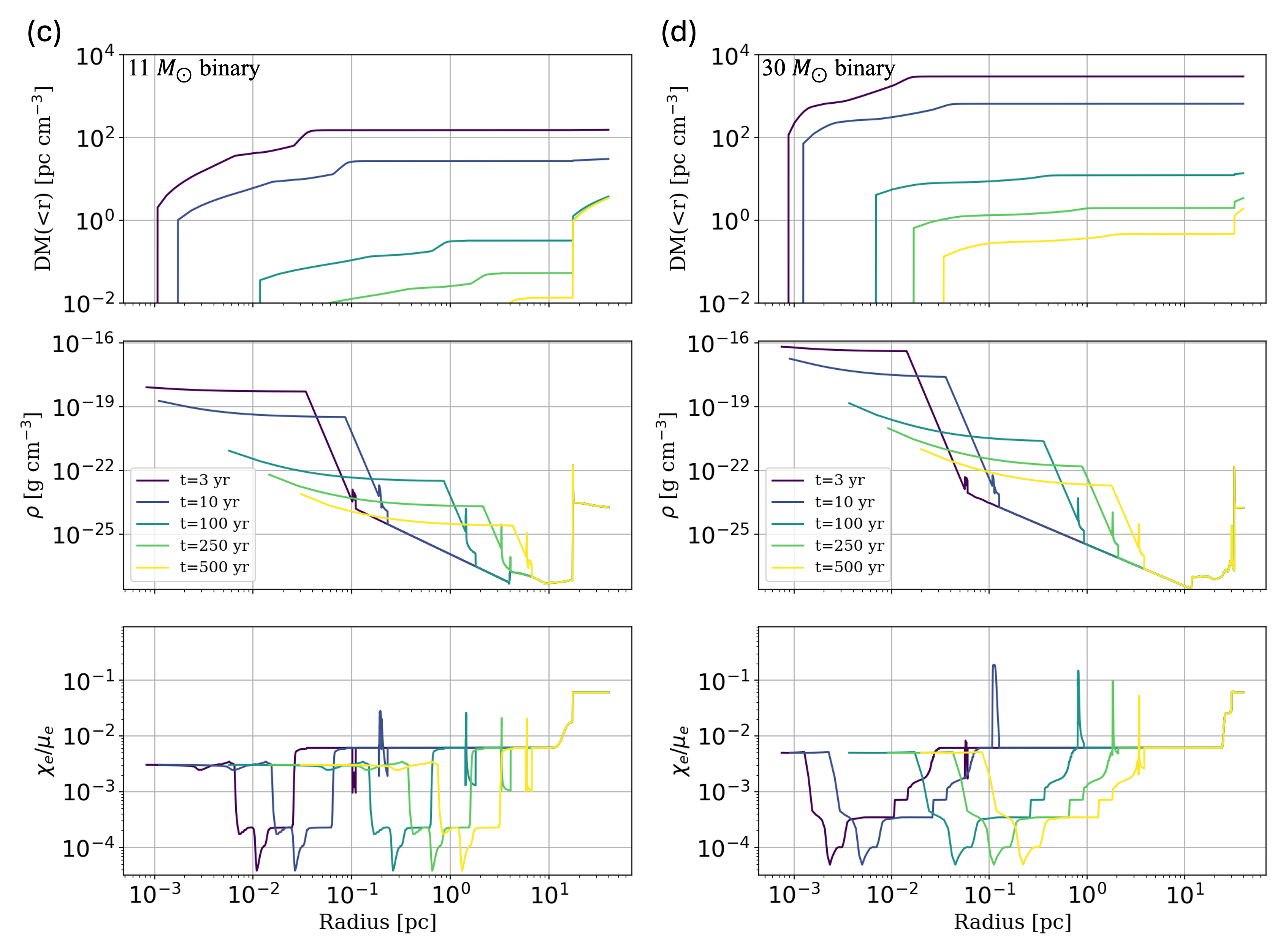
Figure 6 provides an independent cross-check of the above interpretation by showing the radial cumulative DM (top panels) together with the corresponding mass-density (middle panels) and ionization-fraction (bottom panels) profiles at several representative epochs. To facilitate comparison with analytic expectations, we interpret the radial structure in a set of characteristic regimes, starting from the density profiles.

1. Inner-core region. As an illustrative example, we focus on $t=3\,$yr (the initial condition of our SNR calculations). At this epoch, the ejecta are extremely dense and retain a core–envelope structure close to the adopted ejecta profile (Eq. B6), i.e., an approximately flat (nearly uniform) inner core surrounded by a steeply declining power-law envelope. As the remnant evolves, the inner-core region gradually develops a modest radial gradient (i.e., a weak decrease with radius). In the inner-core region, the cumulative DM therefore rises rapidly at small radii and is dominated by the unshocked ejecta.

2. Rapidly declining unshocked-ejecta envelope. Outside the nearly uniform core, the unshocked ejecta enter a steep power-law envelope (with the initial decline set by the ejecta index $n$). The density therefore decreases rapidly with radius, and the cumulative DM correspondingly flattens once the line of sight exits the core.

3. Shocked region. After the unshocked-ejecta envelope, the profiles enter the shocked layer. Although the shocked plasma is highly ionized (see $\chi_{e}$), its DM contribution remains small because the shocked region has a limited path length and a comparatively low mass density, consistent with the decomposition in Fig. 5.

4. Wind-dominated region (pre-SN wind$\times$CSM). Outside the shocked layer, the density profile transitions to the circumstellar environment shaped by pre-SN mass loss, exhibiting an approximately wind-like scaling $\rho\propto r^{-s}$ over a broad radial range (with $s=2$ in most analytic wind models).

5. Pre-SN wind–CSM interaction morphologies: SS vs. BS. “Beyond the wind-like region, the SS and BS channels develop distinct pre-SN wind–CSM interaction morphologies, including a hot cavity excavated by fast winds and density bumps produced by fast–slow wind interactions.

   • SS channel: hot bubble + “double” wall + WR-driven bump. In the SS models (Fig. 6a,b), the hot bubble is primarily generated by the interaction between the fast OB-type wind and the ambient ISM: the OB wind sweeps up the ambient medium into an outer dense shell (“ISM wall”), while the reverse shock propagating back into the wind heats the shocked wind material and inflates a high-pressure hot bubble. At later stages, the dense and slower RSG wind is confined by the hot-bubble thermal pressure, producing an additional inner density enhancement (“bubble wall”). A WR wind, when present (in the $30\,M_{\odot}$ case), can interact with the RSG wind and imprint a modest bump in the cavity profile.

   • BS channel: ISM wall + WR-like bump(with an absent/weak bubble wall). In the BS models (Fig. 6c,d), the H envelope is stripped quickly, so the progenitor largely skips the RSG-wind stage (especially in the $11\,M_{\odot}$ case) and the evolution is dominated by a WR-like He-star wind, broadly similar to the WR-wind phase in the $30\,M_{\odot}$ SS model. In the $30\,M_{\odot}$ BS case in particular, a brief yet physical RSG-like slow-wind phase can still occur and form an inner “bubble wall,” but the subsequent WR-like fast wind rapidly disrupts this structure and drives it outward, leaving it nearly coincident with the “ISM wall” and thus hard to distinguish in the radial profiles. The remaining prominent feature is typically a WR-like bump.

6. Outer ambient ISM: late-time growth of the cumulative DM. At sufficiently large radii—beyond the wind-bubble structure—the ambient medium approaches an approximately constant density. At early times ($t\sim 3$–$10\,$yr) this outer material contributes little to the cumulative DM, whereas at late times ($t\gtrsim 100\,$yr) the declining ejecta density becomes comparable to that of the ambient medium and the cumulative DM can increase again toward the outer boundary.

V.2.2 The derivatives of DM

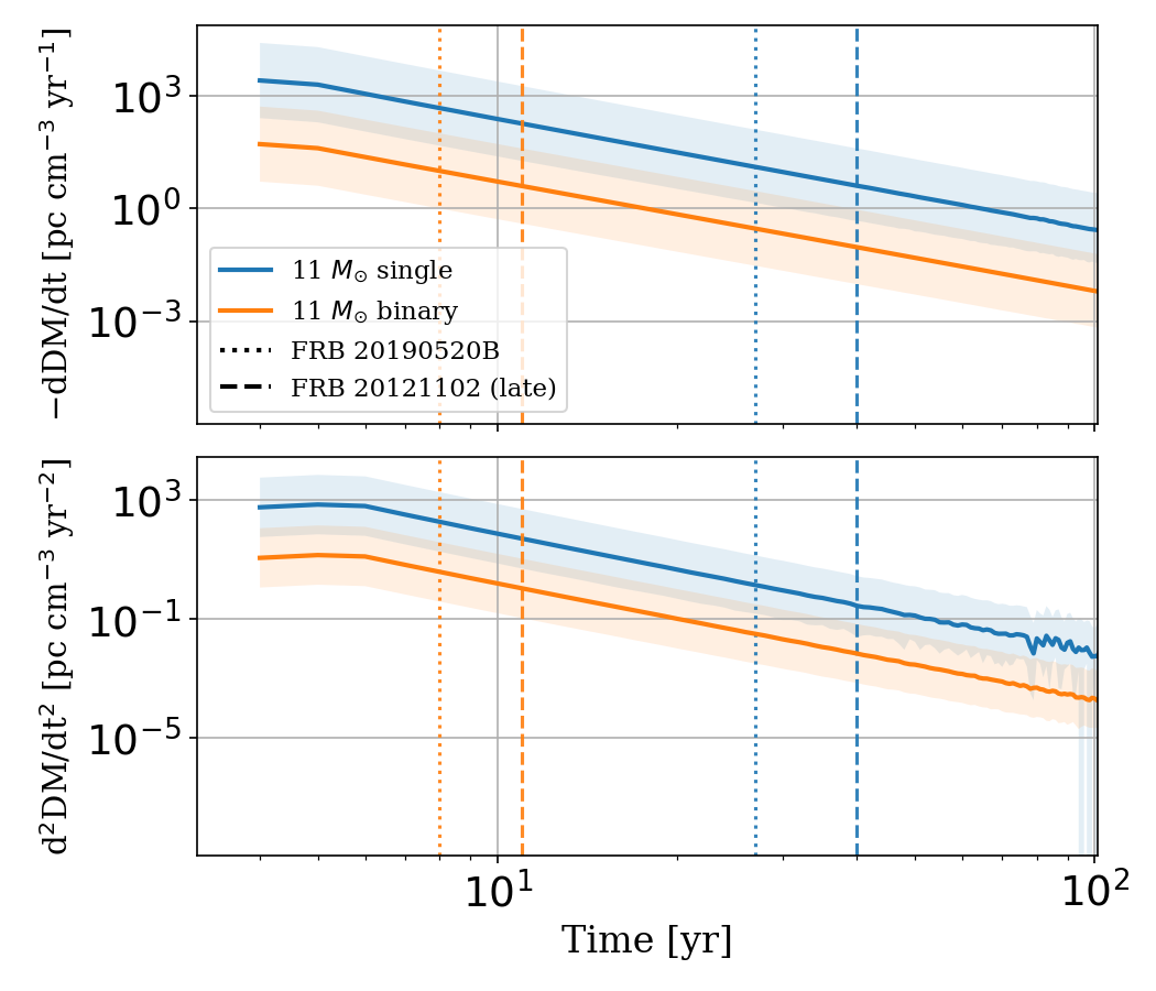
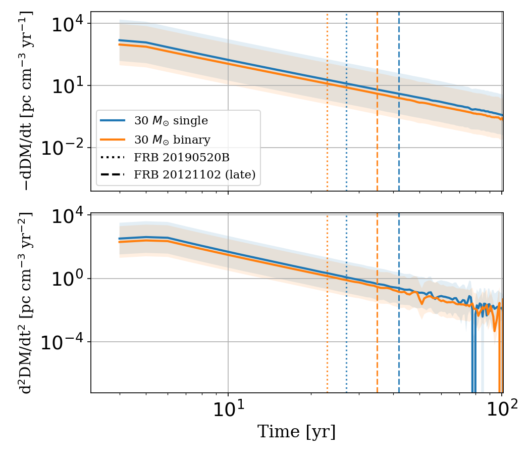
To characterize the secular evolution of ${\rm DM}_{\rm SNR}(t)$ and identify the observational time window in which an FRB can exhibit a measurable DM drift, we compute the first and second time derivatives of the simulated DM using Eq. (20). Figure 7 shows that both ${\rm dDM}/{\rm d}t$ and ${\rm d}^{2}{\rm DM}/{\rm d}t^{2}$ approximately follow a power-law decline in time over the smooth part of the evolution. At $t\gtrsim 100\,$yr, small-amplitude fluctuations become visible, and they are especially prominent in the second derivative. This behavior is expected because finite-difference estimates of higher-order derivatives amplify snapshot-to-snapshot irregularities in ${\rm DM}(t)$; physically, additional non-smooth features can also be introduced when the shock structure encounters density inhomogeneities (shells/bubbles) in the progenitor-shaped CSM.

Motivated by the observed secular decreases in FRB 20190520B ($\mathrm{dDM}/\mathrm{d}t\simeq-12.4\,{\rm pc\,cm^{-3}\,yr^{-1}}$; Niu2025) and FRB 20121102 ($\mathrm{dDM}/\mathrm{d}t=-3.93\,{\rm pc\,cm^{-3}\,yr^{-1}}$; Wang2025arXiv250715790W), we identify the corresponding time window after the SN explosion at which an FRB would need to occur. We denote this FRB occurrence time as $t_{\rm occur}$, i.e., the elapsed time between the SN explosion and the observed FRB activity. Assuming the DM drift is dominated by the local SNR contribution and using the fiducial parameter values adopted in this section, we find $t_{\rm occur}\simeq 27\,$yr (SS) and $t_{\rm occur}\simeq 8\,$yr (BS) for the $11\,M_{\odot}$ models, and $t_{\rm occur}\simeq 27\,$yr (SS) and $t_{\rm occur}\simeq 23\,$yr (BS) for the $30\,M_{\odot}$ models for FRB 20190520B. For FRB 20121102, the same fiducial matching gives systematically later epochs, $t_{\rm occur}\simeq 40\,$yr (11 SS), $11\,$yr (11 BS), $42\,$yr (30 SS), and $35\,$yr (30 BS). The corresponding fiducial ${\rm DM}_{\rm SNR}$ values for both sources are summarized in Table 2. Notably, the significantly lower DM in the $11\,M_{\odot}$ BS case compared with the other progenitors is primarily driven by its much smaller ejecta mass (see Table 1), which directly lowers the unshocked-ejecta electron column. These values correspond to the very early SNR phase, close to the transition from optically thick to optically thin conditions for GHz radio emission (see Section V.2.3 and Table 3). The short duration of this “ambiguous” phase may naturally contribute to the rarity of FRBs showing a clear SNR-like secular DM signature.

Table 2: Fiducial (HH) local SNR DM values at $t_{\rm occur}$ for FRB 20190520B and FRB 20121102.

Progenitor model	${\rm DM}_{\rm SNR}$ for FRB 20190520B	${\rm DM}_{\rm SNR}$ for FRB 20121102
	(pc cm-3)	(pc cm-3)
$11\,M_{\odot}$ SS	183.6	88.5
$11\,M_{\odot}$ BS	44.9	26.2
$30\,M_{\odot}$ SS	202.8	97.7
$30\,M_{\odot}$ BS	167.5	83.0

The simulated second-derivative DM curvature evaluated at $t_{\rm occur}$ is summarized in Table 3 for FRB 20190520B and in Appendix Table 5 for FRB 20121102. At these early epochs, the curvature for FRB 20190520B is typically $\mathrm{d}^{2}{\rm DM}/\mathrm{d}t^{2}\sim 1$–$4\,{\rm pc\,cm^{-3}\,yr^{-2}}$ across the four models, while for FRB 20121102 it is generally smaller, $\sim 0.1$–$1.4\,{\rm pc\,cm^{-3}\,yr^{-2}}$. Following the order-of-magnitude estimate used by Niu2025, we define $\left|\mathrm{d}^{2}{\rm DM}/\mathrm{d}t^{2}\right|_{\rm est}\equiv\alpha\,|\mathrm{dDM}/\mathrm{d}t|/t_{\rm SNR}$ and evaluate it using $t_{\rm SNR}\simeq t_{\rm occur}$. For both FRB 20190520B and FRB 20121102, the estimator remains consistent with the simulated trends at the factor-of-few level, with agreement within $\sim 1.1$–$1.6$.

Figure 7: Time evolution of the DM time derivative in the full-region calculation for the $11\,M_{\odot}$ (left) and $30\,M_{\odot}$ (right) models. For the fiducial (HH) configuration, $t_{\rm occur}$ for FRB 20190520B (Table 3) is $27$ (SS) and $8$ (BS) yr for $11\,M_{\odot}$, and $27$ (SS) and $23$ (BS) yr for $30\,M_{\odot}$; for FRB 20121102 (Table 5), it is $40$ (SS) and $11$ (BS) yr for $11\,M_{\odot}$, and $42$ (SS) and $35$ (BS) yr for $30\,M_{\odot}$.

Figure 8: Time evolution of the optical depth in the full region for the $11\,M_{\odot}$ (left) and $30\,M_{\odot}$ (right) models, including contributions from free–free absorption and Thomson scattering.

V.2.3 Optical depth evolution in the full region

To assess whether FRB 20190520B and FRB 20121102 can plausibly escape from an SNR environment during the inferred occurrence time $t_{\rm occur}$, we compute the time evolution of the optical depth in the full-region calculation and indicate the epoch at which the system becomes optically thin. Figure 8 shows that at early times the total optical depth is dominated by free–free absorption, so we define the GHz escape time $t_{\rm esc}$ by the condition $\tau_{\rm ff}(t_{\rm esc})=1$.

For the models shown in Figure 8, we find $t_{\rm esc}=13\,$yr for the $11\,M_{\odot}$ SS model and $t_{\rm esc}=17\,$yr for the $30\,M_{\odot}$ SS model. For the $30\,M_{\odot}$ BS model, we find $t_{\rm esc}=13\,$yr. In contrast, the $11\,M_{\odot}$ BS model is essentially transparent from the beginning ($t_{\rm esc}\simeq 0\,$yr; $\tau_{\rm tot}<1$ at all simulated times).

Table 3: Summary of characteristic timescales and DM derivatives evaluated at $t_{\rm occur}$ for different assumed ionization configurations of the unshocked ejecta ($\chi_{e,\rm unej}$) and the unshocked ISM ($\chi_{e,\rm ISM}$).

Ionization config.	Quantity	$11\,M_{\odot}$ SS	$11\,M_{\odot}$ BS	$30\,M_{\odot}$ SS	$30\,M_{\odot}$ BS
FF: $\chi_{e,\rm unej}=1$, $\chi_{e,\rm ISM}=1$	$t_{\rm esc}$ (yr)	32	6	62	46
	$t_{\rm occur}$ (yr)	60	16	65	55
	$\mathrm{d}^{2}{\rm DM}/\mathrm{d}t^{2}$ (pc cm-3 yr-2)	0.65	2.45	0.51	0.73
	$\left|\mathrm{d}^{2}{\rm DM}/\mathrm{d}t^{2}\right|_{\rm est}$ (pc cm-3 yr-2)	0.40	1.50	0.35	0.41
HF: $\chi_{e,\rm unej}=0.1$, $\chi_{e,\rm ISM}=1$	$t_{\rm esc}$ (yr)	13	0	17	13
	$t_{\rm occur}$ (yr)	27	8	27	23
	$\mathrm{d}^{2}{\rm DM}/\mathrm{d}t^{2}$ (pc cm-3 yr-2)	1.40	3.88	1.17	1.40
	$\left|\mathrm{d}^{2}{\rm DM}/\mathrm{d}t^{2}\right|_{\rm est}$ (pc cm-3 yr-2)	0.89	3.01	0.84	0.99
MF: $\chi_{e,\rm unej}=0.01$, $\chi_{e,\rm ISM}=1$	$t_{\rm esc}$ (yr)	5	0	4	0
	$t_{\rm occur}$ (yr)	13	–	11	10
	$\mathrm{d}^{2}{\rm DM}/\mathrm{d}t^{2}$ (pc cm-3 yr-2)	2.60	–	3.28	3.04
	$\left|\mathrm{d}^{2}{\rm DM}/\mathrm{d}t^{2}\right|_{\rm est}$ (pc cm-3 yr-2)	1.84	–	2.06	2.28
FH: $\chi_{e,\rm unej}=1$, $\chi_{e,\rm ISM}=0.1$	$t_{\rm esc}$ (yr)	32	6	62	46
	$t_{\rm occur}$ (yr)	60	16	65	55
	$\mathrm{d}^{2}{\rm DM}/\mathrm{d}t^{2}$ (pc cm-3 yr-2)	0.065	2.45	0.51	0.73
	$\left|\mathrm{d}^{2}{\rm DM}/\mathrm{d}t^{2}\right|_{\rm est}$ (pc cm-3 yr-2)	0.40	1.50	0.35	0.41
HH: $\chi_{e,\rm unej}=0.1$, $\chi_{e,\rm ISM}=0.1$	$t_{\rm esc}$ (yr)	13	0	17	13
	$t_{\rm occur}$ (yr)	27	8	27	23
	$\mathrm{d}^{2}{\rm DM}/\mathrm{d}t^{2}$ (pc cm-3 yr-2)	1.41	3.88	1.17	1.40
	$\left|\mathrm{d}^{2}{\rm DM}/\mathrm{d}t^{2}\right|_{\rm est}$ (pc cm-3 yr-2)	0.89	3.01	0.84	0.99
MH: $\chi_{e,\rm unej}=0.01$, $\chi_{e,\rm ISM}=0.1$	$t_{\rm esc}$ (yr)	5	0	4	0
	$t_{\rm occur}$ (yr)	13	–	11	10
	$\mathrm{d}^{2}{\rm DM}/\mathrm{d}t^{2}$ (pc cm-3 yr-2)	2.59	–	3.28	3.03
	$\left|\mathrm{d}^{2}{\rm DM}/\mathrm{d}t^{2}\right|_{\rm est}$ (pc cm-3 yr-2)	1.84	–	2.06	2.28

• In the ionization configuration labels, H/M/L denote High/Middle/Low ionization levels, and F denotes Fully ionized.

• $t_{\rm occur}$ is determined by matching the observed DM derivative of FRB 20190520B, i.e., imposing $\mathrm{dDM}/\mathrm{d}t=-12.4\,$pc cm^-3 yr^-1. “–” indicates that no solution for $t_{\rm occur}$ exists under this condition for the stated ionization assumption.

• $t_{\rm esc}$ is defined by $\tau_{\rm ff}(t_{\rm esc})=1$; $t_{\rm esc}=0$ indicates the model is transparent at all simulated times.

V.3 RM results

The RM and magnetic-field evolutions are shown in Fig. 9. In this shocked-region-only RM framework, only the $11\,M_{\odot}$ SS model reproduces the observed RM range and decay trend of FRB 20121102; the $30\,M_{\odot}$ SS model and both BS models remain below the data and do not satisfy the joint amplitude–slope constraints.

The strong RM contrast between SS and BS models is physically consistent with the shocked-shell dynamics discussed in Section V.1. In particular, the dominant driver is the large difference in shocked mass $M_{\rm sh}$ (Fig. 2e), which translates into a large density contrast in the shocked region. Although BS models can have a higher shock velocity $v_{\rm sh}$ in a more rarefied environment (Fig. 2d), this does not compensate for their much lower shocked density. As a result, the ram pressure $\rho v_{\rm sh}^{2}$—and hence the amplified magnetic field in our prescription—remains significantly smaller than in SS models. In addition, the denser SS shocked layer produces a substantially higher post-shock electron density $n_{e}$ (see Fig. 2b), which further boosts $\int n_{e}B_{\parallel}\,\mathrm{d}l$ and amplifies the final RM separation between SS and BS channels.

Therefore, in a deliberately conservative sense, if we include only magnetic-field amplification in the SNR shock region and neglect other nonlinear effects or additional magnetic/ionization enhancement (e.g., from a MWN or photoionization), the current RM data for FRB 20121102 select the $11\,M_{\odot}$ SS case as the only successful model in our grid, despite studies arguing for a strong MWN environment for this source (Beloborodov2017; Yang2019).

Figure 9: Time evolution of RM and magnetic field for the $11\,M_{\odot}$ (left) and $30\,M_{\odot}$ (right) models, with the FRB 20121102 RM data mapped onto the model time axis (see text). In the top panels, blue circles denote RM measurements from Hilmarsson2021, while red circles denote the newly added RM measurements from Wang2025arXiv250715790W. The top panels show RM evolution, and the bottom panels show magnetic-field evolution, where $\langle B_{\rm sh}\rangle$ is the electron-density-weighted mean field in the shocked region. Shaded bands mark the observed RM range and the allowed $\langle B_{\rm sh}\rangle$ range.

V.4 Simulation v.s. analytic models

Table 4: Physical parameters adopted in different analytic/semi-analytic DM prescriptions.

Model	Parameters in formula	Adopted values
YZ17: ionized ejecta (FE; Eq. 4)	$M_{1},\,E_{51},\,\chi_{e},\,\mu_{m}$	$\mu_{m}=1.2$
PG18: shocked ionized (Eq. 5–6)	$M_{1},\,E_{51}$ shared ISM: $n_{0},\,\mu_{m},\,\mu_{e}$ wind: $\mu_{e},\,K(\dot{M},v_{w})$	ISM: $n_{0}=1\penalty 10000\ \mathrm{cm^{-3}}$ SS: $\mu_{m}=0.62,\,\mu_{e}=1.18$ BS: $\mu_{m}=1.34,\,\mu_{e}=2.0$ wind: $\dot{M}=10^{-5}\,M_{\odot}\,\mathrm{yr^{-1}}$ $v_{w}=10\penalty 10000\ \mathrm{km\,s^{-1}}$
Zhao+2021: SSDW wind (Eq. 8–12)	$M_{\rm ej},\,E_{51},\,n,\,s,$ $\mu_{a},\,\chi_{e},\,\dot{M},\,v_{w}$	$n=10,\ s=2$ $w_{\rm core}=0.1,\ \mu_{a}=1$ $\dot{M}=10^{-5}\,M_{\odot}\,\mathrm{yr^{-1}}$ $v_{w}=10\penalty 10000\ \mathrm{km\,s^{-1}}$

Figure 10: Time evolution of the SNR DM comparing numerical simulations with analytic expectations. Left panels show $11\,M_{\odot}$ models and right panels show $30\,M_{\odot}$ models; the top row corresponds to SS progenitors and the bottom row to BS progenitors. The “upper limit” curve assumes that the entire SNR material is fully ionized and that the ejecta are composed purely of hydrogen. For Zhao+21 and YZ17, we adopt the fiducial assumption $\chi_{e,\mathrm{unsh}}=0.1$

Fig. 10 compares the DM evolution obtained from our numerical SNR simulations with several commonly adopted analytic prescriptions. Hereafter, we denote Yang&Zhang2017 as YZ17 and Piro&Gaensler2018 as PG18.

We evaluate the analytic prescriptions using the same explosion and wind parameters adopted in our progenitor setup (Table 1). For the remaining analytic-model parameters, we follow the values adopted in the original literature where they are explicitly specified (Table 4). Here we only restate the mathematical definitions: $n_{e}=\rho/(\mu_{e}m_{p})$, $n_{\rm tot}=\rho/(\mu_{m}m_{p})$, and $\mu_{a}=\sum_{i}n_{i}A_{i}/\sum_{i}n_{i}$, where $n_{\rm tot}$ denotes the total particle number density (ions + electrons).

For specific models, Yang&Zhang2017 adopt $\mu_{m}=1.2$ (solar-composition, approximately neutral material), while ZYZhao2021b state $\mu_{a}\simeq 1$ for their fiducial H-dominated ejecta. When required, we compute $\mu_{a}$ directly from the simulated elemental composition. For the PG18 analytic curves, which do not explicitly state $\mu_{m}$ or $\mu_{e}$, we adopt fiducial composition assumptions; for a fully ionized H/He mixture, where $X$ and $Y$ are the hydrogen and helium mass fractions ($X+Y=1$), the standard relations are $\mu_{e}=2/(1+X)$ and $\mu_{m}=1/(2X+3Y/4)$. We then use: (i) SS case with H+He-dominated ejecta, $X\simeq 0.7$, $Y\simeq 0.3$, giving $\mu_{m}\simeq 0.62$ and $\mu_{e}\simeq 1.18$; (ii) BS case with He-dominated ejecta (H envelope lost), giving $\mu_{m}\simeq 1.34$ and $\mu_{e}\simeq 2.0$. These adopted values are the ones used in our PG18 comparisons.

We also evaluate the analytic prescriptions using the simulated, composition-dependent $\mu_{a}$, $\mu_{e}$, and $\mu_{m}$. These results are presented in Appendix C and Fig. 13.

In Fig. 10, the black dashed curve denotes the upper limit, which assumes H-dominated unshocked ejecta and CSM ($\mu_{e}=\mu_{a}=1$) that are fully ionized ($\chi_{e}=1$). Among the cases shown, the largest deviation from the numerical results occurs for the shocked-ionized ejecta scenario, whereas most analytic prescriptions fall within the upper and lower envelopes of our DM evolution. Under our fiducial assumptions in Fig. 10, YZ17 most closely matches the $11\,M_{\odot}$ SS case, while the PG18 wind case is closer for the $30\,M_{\odot}$ SS case. These "best-match" identifications are dependent on progenitor-model choices and parameter assumptions and are not intended to indicate a general preference among analytic prescriptions. Notably, when we adopt simulation-based, composition-dependent $\mu_{a}$, $\mu_{e}$, and $\mu_{m}$ (Fig. 13), the $11\,M_{\odot}$ SS case becomes more consistent with the Zhao+2021 prediction.

Using the $t_{\rm occur}$ values constrained by Fig. 7, we obtain the corresponding ${\rm DM}_{\rm SNR}$ values of $183.6\,{\rm pc\,cm^{-3}}$ ($11\,M_{\odot}$ SS), $202.8\,{\rm pc\,cm^{-3}}$ ($30\,M_{\odot}$ SS), $44.9\,{\rm pc\,cm^{-3}}$ ($11\,M_{\odot}$ BS), and $167.5\,{\rm pc\,cm^{-3}}$ ($30\,M_{\odot}$ BS). This indicates that the DM constraint varies significantly not only with model parameters but also with progenitor channel. Nevertheless, all inferred contributions lie in the tens-to-hundreds ${\rm pc\,cm^{-3}}$ range, representing a non-negligible extra component that can materially affect FRB cosmological analyses.

V.5 Shocked-region electron source and ionization states

In addition to the total DM_sh, our simulations track the contribution to the electron density from different elements and ionization stages in the shocked region physically.

Figure 11: Radial profiles in the shocked region at the DM_sh peak, showing number densities of electrons (red) and selected elements for the four models considered in this work. The cyan and blue curves correspond to H and He, respectively.

Fig. 11 shows the radial number-density profiles in the shocked region at the DM_sh peak (see Fig. 2a). A clear channel dependence is visible: in the SS models, the shocked composition is generally H-rich with He as the secondary contributor, whereas in the BS models He dominates and metals remain subdominant. Notably, compared with the $11\,M_{\odot}$ SS model, the $30\,M_{\odot}$ SS model has a smaller hydrogen fraction and is therefore more Type IIb-like than a typical H-rich Type IIP case. This difference ultimately reflects the distinct progenitor-envelope structures: SS ejecta are largely composed of the progenitor’s H-rich envelope, while in the BS channel binary interaction efficiently removes the H envelope prior to core collapse (e.g., via common-envelope evolution and Roche-lobe overflow), leaving a He-rich progenitor whose ejecta contain comparatively little H. As a result, in the BS models the post-shock electron budget is primarily supplied by ionized He, whereas in the SS models it is dominated by ionized H.

This composition difference also helps explain why the BS models reach a larger $\langle Z\rangle$ at the peak (bottom panels of Fig. 3) than the SS models: helium can contribute up to two electrons per ion once ionized, raising the typical ionic charge and hence $\langle Z\rangle$ relative to an H-dominated composition.

This interpretation is further supported by the ionization-state structure of the shocked region in Fig. 12: in panel (a), corresponding to the $11\,M_{\odot}$ SS model, the peak number density of H⁺ exceeds that of He²⁺, whereas in panel (b), corresponding to the $11\,M_{\odot}$ BS model, the shocked region is instead dominated by He⁺ and He²⁺.

(a) $11\,M_{\odot}$ SS

(b) $11\,M_{\odot}$ BS

Figure 12: Ionization-state profiles in the shocked region at $t=30\,\mathrm{yr}$ for the $11\,M_{\odot}$ SS and BS models.

VI Model Limitations and Future Directions

In this section, we outline some of the main implications of our preliminary results and discuss directions for future refinement.

• The ionization and thermal evolution history of the unshocked ejecta is treated approximately in the current setup. In particular, we do not yet include a fully self-consistent ionization–recombination balance, nor possible CCO-related heating/ionization channels, in the unshocked region. This limitation introduces a relatively broad uncertainty when constraining source-environment parameters from DM evolution, and should be improved in future work.

• In our current 1D SNR simulations we do not enable cosmic-ray (CR) acceleration and transport. As a result, potentially important CR-related processes—including escaping CR particles and CR-driven magnetic-field amplification (e.g., streaming instabilities and Bell-type instabilities)—are absent. Incorporating these effects in future calculations may provide new physical insight into the magnitude and time evolution of RM.

• The present 1D framework assumes spherical symmetry and a stationary central engine. Real SNR evolution is intrinsically 3D and often asymmetric: binary stripping through Roche-lobe overflow is non-spherical, the SN explosion and external CSM can be nonuniform and anisotropic, and a young magnetar may have a substantial natal kick velocity. In addition, the binary-stripped channel considered here represents only one pathway within a much broader binary-interaction parameter space (e.g., different mass ratios, orbital separations, mass-transfer histories, and common-envelope outcomes). These effects can produce significant sightline-to-sightline variance in shell structure, and therefore in DM and RM. Extending the model toward multidimensional calculations and a broader binary-model grid will be essential to quantify these geometric and progenitor-channel systematics.

• The apparent rarity of FRBs with a clear SNR-like secular DM signature can be naturally understood as a short observational window effect, consistent with the population-level transient-association and timescale arguments presented by Dong2025.

VII Summary

In this paper, we develop a framework to quantify the local SNR contribution to FRB DM using 1D HD+NEI simulations for both $11\,M_{\odot}$ and $30\,M_{\odot}$ progenitors in single-star (SS) and binary-stripped (BS) channels. Our main conclusions are as follows.

• Considering only the shocked region, the DM contribution is limited (${\lesssim}10\,{\rm pc\,cm^{-3}}$) and is especially negligible for BS models. By contrast, even under this conservative setup—using the simulated shocked-plasma ionization state and ram-pressure-based magnetic amplification—the predicted RM can still reach the high values observed in FRB 20121102 for the $11\,M_{\odot}$ SS model. Within our model grid, this shocked-region RM comparison selects only the $11\,M_{\odot}$ SS case and disfavors the $30\,M_{\odot}$ SS and BS progenitor models as primary explanations of the FRB 20121102 RM data.

• For DM evolution, the dominant contribution comes from the unshocked ejecta. Its early-time decline is governed by free expansion and follows ${\rm DM}\propto t^{-\alpha}$ with $\alpha\simeq 1.8$–$1.9$ (slightly shallower than 2), while the late-time behavior transitions toward a regime increasingly influenced by the approximately constant-density ambient ISM/CSM contribution.

• BS models generally yield smaller DM than SS models at the same $M_{\rm ZAMS}$ because H-envelope stripping reduces ejecta mass and therefore the available electron column in the unshocked ejecta, which dominates ${\rm DM}_{\rm SNR}$ in our simulations. This SS–BS contrast is additionally modulated by reverse-shock development and CSM structure: BS models (and also the massive SS model) can evolve in lower-density wind-blown cavities, delaying strong reverse-shock formation at ages of a few hundred years and further reducing the shocked-ejecta DM contribution.

• The total optical depth is generally dominated by free–free absorption. Using the condition $\tau_{\rm ff}=1$, we infer $t_{\rm esc}\lesssim 70\,$yr across the explored ionization configurations. For weakly ionized ejecta ($\chi_{e,\rm unej}\sim 0.01$), the SNR is nearly transparent to FRB emission from very early times.

• Using the observed DM decay rates of FRB 20190520B and FRB 20121102 to constrain $t_{\rm occur}$, we find $t_{\rm occur}\lesssim 100\,$yr (measured from the SN explosion) in all fiducial models, and FRB 20121102 consistently occurs later than FRB 20190520B within the same progenitor model; in the great majority of cases, both sources can be transparent to GHz FRB escape.

• The mass dependence is not always monotonic. In our models, DM is dominated by weakly ionized unshocked ejecta, so under the low-ionization assumption (approximately fixed $\chi_{e}$, effectively at most one free electron per atom), larger mean atomic/electron weights in metal-rich ejecta can reduce $n_{e}$ and produce non-monotonic trends across progenitors. This behavior can change or even reverse when the reverse shock penetrates more ejecta and/or reverse-shock-related radiation (photoionization/PR) further ionizes heavy elements, increasing the electron yield.

• A common conclusion from both FRB 20190520B and FRB 20121102 is that the inferred local SNR contribution falls in the tens-to-hundreds ${\rm pc\,cm^{-3}}$ range. At the fiducial-value $t_{\rm occur}$ constrained from the observed DM slopes, the inferred ${\rm DM}_{\rm SNR}$ shows a clear model split for both sources: for FRB 20190520B, the $11\,M_{\odot}$ BS model gives only $\sim 44.9\,{\rm pc\,cm^{-3}}$, while the other models are $\sim 200\,{\rm pc\,cm^{-3}}$; for FRB 20121102, the $11\,M_{\odot}$ BS model gives $\sim 26.2\,{\rm pc\,cm^{-3}}$, while the others are $\sim 100\,{\rm pc\,cm^{-3}}$. The significantly smaller DM in the $11\,M_{\odot}$ BS case is mainly due to its much smaller ejecta mass. Therefore, the early CCSN/SNR local contribution to ${\rm DM}_{\rm source}$ is non-negligible and can materially affect FRB cosmological inferences.

• For FRB 20121102, the coexistence of strong RM evolution and a two-stage DM-slope evolution (early weak rise and late decline) suggests that a pure single-component interpretation is incomplete. A hybrid SNR+MWN picture is favored, where the late-time DM decline is consistent with SNR expansion while additional local plasma from MWN-related processes can contribute to the early-stage slope turnover and magneto-ionic variability.

These results underscore the need for physically consistent choices of progenitor and local-environment models when estimating and marginalizing the local DM term in FRB cosmology. Future work will expand the progenitor grid and include additional local components (e.g., MWN and host H II regions) to further tighten constraints on ${\rm DM}_{\rm source}$.

Data Availability

The data presented in this paper is available to the research community upon request to the authors.

Appendix A Gaunt Factor for Free–Free Absorption

The free–free absorption coefficient used in Eq. (6) depends on the velocity–averaged Gaunt factor $g_{\rm ff}(\nu,T_{\rm e},Z)$, which corrects the classical bremsstrahlung cross section for quantum and kinematic effects. The asymptotic behavior of the Gaunt factor was derived by NovikovThorne1973 and later summarized in Fig. 5.2 of RybickiLightman1979. Its dependence can be expressed in terms of two dimensionless parameters:

$$u=\frac{h\nu}{k_{\rm B}T_{\rm e}},\qquad\eta=\frac{k_{\rm B}T_{\rm e}}{Z^{2}R_{\rm y}},$$ (A1)

where $R_{\rm y}=13.6{\rm\,eV}$ is the Rydberg energy.

The Gaunt factor admits three analytic limits:

(1) Large–angle region

The transition to large–angle Rutherford scattering occurs when the impact parameter reaches the regime where

$$1\;\gtrsim\;u\;\gtrsim\;\eta^{1/2}.$$ (A1)

In this regime the Gaunt factor is of order unity,

$$g_{\rm ff}^{\rm(LA)}\simeq 1.$$ (A2)

(2) Small–angle classical region ($u\ll 1$ and $\eta<1$)

$$g_{\rm ff}^{\rm(cl)}=\frac{\sqrt{3}}{\pi}\ln\!\left[\frac{1}{2\,\xi^{5/2}}\left(\frac{k_{\rm B}T_{\rm e}}{Z^{2}R_{\rm y}}\right)^{1/2}\left(\frac{k_{\rm B}T_{\rm e}}{h\nu}\right)\right],$$ (A3)

where $\xi=e^{\gamma}\simeq 1.781$ and $\gamma$ is Euler’s constant.

(3) Small–angle U.P. region ($u\ll 1$ and $\eta>1$)

$$g_{\rm ff}^{\rm(UP)}=\frac{\sqrt{3}}{\pi}\ln\!\left[\frac{1}{\xi^{2}}\left(\frac{k_{\rm B}T_{\rm e}}{h\nu}\right)\right].$$ (A4)

Because the SNR spans a broad range of temperatures ($T_{\rm e}\sim 10^{4}$–$10^{7}$ K) and the FRB frequencies lie in the GHz band, different radial layers naturally fall into different asymptotic regimes. To ensure numerical smoothness, we evaluate the Gaunt factor using a blended interpolation across the boundaries $u=\eta^{1/2}$ and $\eta=1$. Throughout this work, we compute $g_{\rm ff}$ at $\nu=10^{9}\,{\rm Hz}$.

Appendix B Characteristic Scales and Self-Similar Constants in the Wind Case

In this appendix, we summarize the characteristic scales and dimensionless constants adopted in the self-similar driven wave (SSDW) solution for a supernova remnant (SNR) expanding into a wind-like circumstellar medium (CSM) with density profile $\rho_{\rm w}\propto r^{-2}$ ($s=2$).

B.1 Characteristic Radius and Timescale

For a wind environment characterized by $K\equiv\dot{M}/(4\pi v_{\rm w})$, we define the normalized parameter $K_{13}\equiv K/(10^{13}\,{\rm g\,cm^{-1}})$. Following the standard SSDW scaling (e.g., Tang&Chevalier2017; ZYZhao2021a), the characteristic radius and timescale are given by

$$R_{\rm ch}\simeq 6.58\times 10^{2}\,\mathrm{pc}\;M_{1}\left(\frac{5.1}{K_{13}}\right),$$ (B1)

and

$$t_{\rm ch}\simeq 2.86\times 10^{5}\,\mathrm{yr}\;E_{51}^{-1/2}\,M_{1}^{3/2}\left(\frac{5.1}{K_{13}}\right),$$ (B2)

The numerical factor $5.1$ arises from the fiducial normalization $\dot{M}=10^{-5}\,M_{\odot}\,\mathrm{yr^{-1}}$ and $v_{w}=10\,\mathrm{km\,s^{-1}}$, for which $K\simeq 5.1\times 10^{13}\,\mathrm{g\,cm^{-1}}$. These characteristic scales are used to normalize the self-similar evolution of the forward shock, reverse shock, and contact discontinuity.

B.2 Contact Discontinuity and the Constant $\zeta_{c}$

We follow the standard parametrization of the ejecta and ambient-medium density profiles (e.g., TM99), writing

$$\rho(r,t)=\begin{cases}\rho_{\rm ej}(r,t),&r\leq R_{\rm ej}(t),\\[4.0pt] \rho_{\rm a}(r),&r>R_{\rm ej}(t),\end{cases}$$ (B3)

where the ambient medium is described by a power law

$$\rho_{\rm a}(r)=\eta_{s}\,r^{-s},$$ (B4)

and the freely expanding ejecta take the form

$$\rho_{\rm ej}(r,t)=\frac{M_{\rm ej}}{R_{\rm ej}^{3}(t)}\,f\!\left(\frac{r}{R_{\rm ej}(t)}\right).$$ (B5)

Here $R_{\rm ej}(t)$ is the outer radius of the ejecta and $w\equiv r/R_{\rm ej}$. The ejecta structure function $f(w)$ is specified by a flat inner core and a power-law outer envelope,

$$f(w)=\begin{cases}f_{0},&0\leq w\leq w_{\rm core},\\[4.0pt] f_{0}\left(\dfrac{w_{\rm core}}{w}\right)^{n},&w_{\rm core}\leq w\leq 1,\end{cases}\qquad(n>5),$$ (B6)

where $w_{\rm core}$ denotes the fractional core radius and $n$ is the outer power-law index of the ejecta. The normalization constant $f_{0}$ is fixed by the mass conservation condition $\int_{0}^{1}4\pi w^{2}f(w)\,dw=1$, yielding

$$f_{0}=\frac{3}{4\pi w_{\rm core}^{n}}\left[\frac{1-n/3}{1-(n/3)\,w_{\rm core}^{\,3-n}}\right].$$ (B7)

The radius of the contact discontinuity can be written as (Tang&Chevalier2017)

$$R_{c}^{*}(t^{*})=\left[\left(\lambda_{c}\,t^{*}\right)^{-\tilde{\alpha}}+\left(c\,t^{*\beta}\right)^{-\tilde{\alpha}}\right]^{-1/\tilde{\alpha}},$$ (B8)

where $R_{c}^{*}\equiv R_{c}/R_{\rm ch}$ and $t^{*}\equiv t/t_{\rm ch}$. Here $\tilde{\alpha}$ is the interpolation exponent in the fitting formula of Tang&Chevalier2017 and is unrelated to the DM time-scaling index $\alpha$ (defined in the main text via ${\rm DM}\propto t^{-\alpha}$). This expression interpolates between the early-time free-expansion behavior $R_{c}^{*}\simeq\lambda_{c}t^{*}$ and the self-similar ejecta-dominated regime $R_{c}^{*}\simeq c\,t^{*\beta}$, with $\beta=(n-3)/(n-s)$. In the SSDW limit ($t\ll t_{\rm ch}$), $R_{c}$ reduce to

$$R_{c}(t)\simeq\zeta_{c}\,R_{\rm ch}\left(\frac{t}{t_{\rm ch}}\right)^{\frac{n-3}{n-s}},$$ (B9)

where $s=2$ for the wind case. The dimensionless normalization constant $\zeta_{c}$ encapsulates the detailed structure of the self-similar solution and is given by

$$\zeta_{c}=\left(A\,f_{0}\,w_{\rm core}^{\,n}\,\lambda_{c}^{\,n-3}\right)^{\frac{1}{n-s}}.$$ (B10)

where the constant $A$ is a dimensionless coefficient that depends on $(n,s)$, with values tabulated in Chevalier1982. In this work, we adopt $A=0.067$, corresponding to $n=10$ and $s=2$. The parameter $\lambda_{c}$ is a dimensionless constant related to the density profile of the ejecta and can be expressed as

$$\lambda_{c}^{2}=2\,w_{\rm core}^{-2}\left(\frac{5-n}{3-n}\right)\left(\frac{w_{\rm core}^{\,n-3}-n/3}{w_{\rm core}^{\,n-5}-n/5}\right).$$ (B11)

Appendix C Analytic-Model Comparison Using Simulated Mean Molecular Weights

In these appendix figures, the analytic prescriptions are evaluated using the composition-dependent quantities extracted from the simulations. For the unshocked ejecta and unshocked CSM we adopt $\mu_{a}$, under the assumption that each atom in the unshocked ejecta contributes only one free electron (hence $\mu_{e}=\mu_{a}$), while for the shocked region we use $\mu_{e}$ and $\mu_{m}$ computed from the self-consistent ionization evolution. In the PG18 wind case, the time-dependent $\mu_{e}(t)$ in the shocked region introduces an early-time variation that is qualitatively consistent with the NEI features seen in our shocked-region simulations. By contrast, the PG18 shocked-ionized case shows a nearly negligible NEI imprint because the DM evolution depends primarily on the ratio $\mu_{m}/\mu_{e}$ (see Eq. 6); this ratio varies less than $\mu_{e}$ or $\mu_{m}$ individually, thereby suppressing the apparent ionization-driven modulation in ${\rm DM}(t)$.

Figure 13: Same format as Fig. 10, but the analytic prescriptions adopt the simulated mean molecular weights ($\mu_{a},\,\mu_{e},\,\mu_{m}$) for each model, rather than the fiducial values used in Section V.4.

Appendix D Occurrence-Time and Curvature Table for FRB 20121102

In this appendix table, $t_{\rm occur}$ and the DM-derivative quantities are evaluated at the epoch where $\mathrm{dDM}/\mathrm{d}t=-3.93\,{\rm pc\,cm^{-3}\,yr^{-1}}$, corresponding to the second-stage DM evolution of FRB 20121102.

Table 5: Same format as Table 3, but for FRB 20121102. Here $t_{\rm occur}$ and DM-derivative quantities are defined at $\mathrm{dDM}/\mathrm{d}t=-3.93\,{\rm pc\,cm^{-3}\,yr^{-1}}$ (the second-stage DM evolution of FRB 20121102).

Ionization config.	Quantity	$11\,M_{\odot}$ SS	$11\,M_{\odot}$ BS	$30\,M_{\odot}$ SS	$30\,M_{\odot}$ BS
FF: $\chi_{e,\rm unej}=1$, $\chi_{e,\rm ISM}=1$	$t_{\rm esc}$ (yr)	32	6	62	46
	$t_{\rm occur}$ (yr)	87	24	98	84
	$\mathrm{d}^{2}{\rm DM}/\mathrm{d}t^{2}$ (pc cm-3 yr-2)	0.21	0.50	0.15	0.10
	$\left|\mathrm{d}^{2}{\rm DM}/\mathrm{d}t^{2}\right|_{\rm est}$ (pc cm-3 yr-2)	0.09	0.33	0.07	0.09
HF: $\chi_{e,\rm unej}=0.1$, $\chi_{e,\rm ISM}=1$	$t_{\rm esc}$ (yr)	13	0	17	13
	$t_{\rm occur}$ (yr)	40	11	42	35
	$\mathrm{d}^{2}{\rm DM}/\mathrm{d}t^{2}$ (pc cm-3 yr-2)	0.28	1.07	0.24	0.29
	$\left|\mathrm{d}^{2}{\rm DM}/\mathrm{d}t^{2}\right|_{\rm est}$ (pc cm-3 yr-2)	0.19	0.69	0.17	0.21
MF: $\chi_{e,\rm unej}=0.01$, $\chi_{e,\rm ISM}=1$	$t_{\rm esc}$ (yr)	5	0	4	0
	$t_{\rm occur}$ (yr)	19	5	17	15
	$\mathrm{d}^{2}{\rm DM}/\mathrm{d}t^{2}$ (pc cm-3 yr-2)	0.60	1.43	0.65	0.67
	$\left|\mathrm{d}^{2}{\rm DM}/\mathrm{d}t^{2}\right|_{\rm est}$ (pc cm-3 yr-2)	0.40	1.56	0.45	0.46
FH: $\chi_{e,\rm unej}=1$, $\chi_{e,\rm ISM}=0.1$	$t_{\rm esc}$ (yr)	32	6	62	46
	$t_{\rm occur}$ (yr)	87	24	98	84
	$\mathrm{d}^{2}{\rm DM}/\mathrm{d}t^{2}$ (pc cm-3 yr-2)	0.21	0.50	0.15	0.10
	$\left|\mathrm{d}^{2}{\rm DM}/\mathrm{d}t^{2}\right|_{\rm est}$ (pc cm-3 yr-2)	0.09	0.33	0.07	0.09
HH: $\chi_{e,\rm unej}=0.1$, $\chi_{e,\rm ISM}=0.1$	$t_{\rm esc}$ (yr)	13	0	17	13
	$t_{\rm occur}$ (yr)	40	11	42	35
	$\mathrm{d}^{2}{\rm DM}/\mathrm{d}t^{2}$ (pc cm-3 yr-2)	0.22	1.08	0.24	0.29
	$\left|\mathrm{d}^{2}{\rm DM}/\mathrm{d}t^{2}\right|_{\rm est}$ (pc cm-3 yr-2)	0.20	0.69	0.17	0.21
MH: $\chi_{e,\rm unej}=0.01$, $\chi_{e,\rm ISM}=0.1$	$t_{\rm esc}$ (yr)	5	0	4	0
	$t_{\rm occur}$ (yr)	19	5	17	15
	$\mathrm{d}^{2}{\rm DM}/\mathrm{d}t^{2}$ (pc cm-3 yr-2)	0.60	1.43	0.65	0.67
	$\left|\mathrm{d}^{2}{\rm DM}/\mathrm{d}t^{2}\right|_{\rm est}$ (pc cm-3 yr-2)	0.40	1.56	0.45	0.46