Combinatorial Allocation Bandits with Nonlinear Arm Utility

Abstract

A matching platform is a system that matches different types of participants, such as companies and job-seekers. In such a platform, merely maximizing the number of matches can result in matches being concentrated on highly popular participants, which may increase dissatisfaction among other participants, such as companies, and ultimately lead to their churn, reducing the platform’s profit opportunities. To address this issue, we propose a novel online learning problem, Combinatorial Allocation Bandits (CAB), which incorporates the notion of arm satisfaction. In CAB, at each round $t=1,\dots,T$, the learner observes $K$ feature vectors corresponding to $K$ arms for each of $N$ users, assigns each user to an arm, and then observes feedback following a generalized linear model (GLM). Unlike prior work, the learner’s objective is not to maximize the number of positive feedback, but rather to maximize the arm satisfaction. For CAB, we provide an upper confidence bound algorithm that achieves an approximate regret upper bound, which matches the existing lower bound for the special case. Furthermore, we propose a TS algorithm and provide an approximate regret upper bound. Finally, we conduct experiments on synthetic data to demonstrate the effectiveness of the proposed algorithms compared to other methods.

1 Introduction

Online learning is a framework in which decisions are made sequentially based on observed information. It has a wide range of potential applications, such as recommender systems, and has been studied extensively from a theoretical perspective (Auer et al., 2002a; Cesa-Bianchi and Lugosi, 2006; Li et al., 2010).

Although these studies make important theoretical contributions, they mainly focus on maximizing the number of positive feedback, such as matches or clicks, which sometimes fail to describe real-world business objectives. For example, under unconstrained settings, a match-maximizing algorithm often yields an imbalanced selection of arms, leading to dissatisfaction among infrequently selected arms. In job-matching platforms that recommend companies to visiting users, the revenue model typically relies on fees paid by the companies participating in the platform to hire qualified applicants. Thus, the economic cost of company churn can outweigh raw match counts. Such a structure also appears in dating apps and paper review processes. Dating apps can be viewed as a match between users. When matches concentrate on a small number of highly popular users, many others receive few or no matches, which in turn reduces their incentives to remain active. This decline in active participation is undesirable from the platform’s perspective. Similarly, paper review processes can be regarded as a match between authors and reviewers. If authors are not sufficiently satisfied with the quality of the reviews, they may submit their work to other journals, resulting in a loss of feature submissions.

The key point in the above discussions is that companies whose satisfaction falls below a certain level are expected to have a higher probability of leaving the platform. Here, incorporating principles of economics and the cost of interviewing many applicants, we model each arm’s satisfaction as a concave function of the number of matches it secures. Under this model, it is business-aligned to minimize the number of arms that receive few or no matches and are at risk of churn, rather than to create a small subset of arms that monopolize many matches. As illustrated on the right side of fig. 1, our goal is to ensure that many arms satisfy, even at the cost of reducing the number of matches. Here, satisfaction refers, in the context of a job-matching platform, to the evaluation that a company assigns to the platform, which depends on factors such as the quality and suitability of the users allocated to it. For the functional form, we consider concave functions to capture diminishing marginal utility. By leveraging the concept of satisfaction, we assume that the concentration and dispersion of matches are appropriately balanced, without imposing explicit fairness constraints.

As an illustration of why linear reward maximization may be undesirable, consider the following scenario using fig. 1: an arm is recommended to a user, and the user decides whether to match with the recommended arm. There are $4$ arms, A, B, C, and D, and arm A is assumed to be a ”good” arm that is easy to match with. In this setting, if a goal is to maximize the number of matches, the optimal action is to recommend only arm A, as shown on the left side of fig. 1. Moreover, even for arm A, which receives many assignments, real-world constraints such as budget limits and capacity restrictions, as well as the economic principle of diminishing marginal utility, imply that the satisfaction obtained does not necessarily grow proportionally with the reward.

To address such concentration, several approaches have been considered, including adding constraints to the learning procedure or incorporating fairness. The former contains the bandits with knapsacks (Badanidiyuru et al., 2013; Agrawal and Devanur, 2016; Sankararaman and Slivkins, 2018), which extends the multi-armed bandit by introducing constraints. However, this problem mainly targets situations with well-specified quantitative constraints, such as resource limitations in clinical trials or budget constraints. It thus cannot capture aspects of our interest, such as the satisfaction of arms or the diminishing property of the utility function.

One of the latter approaches is to promote fairness by requiring that each arm be selected at least a certain number of times (Joseph et al., 2016; Li et al., 2019; Xu et al., 2020). While this strategy indeed guarantees a formal notion of fairness in terms of selection counts, it does not take into account which users are assigned to each arm, and thus may not necessarily lead to actual satisfaction. For example, suppose that there are users whose evaluations from the perspective of an arm range from $0.1$ to $0.9$ in increments of $0.1$, and three arms A, B, and C that yield rewards equal to the evaluation multiplied by $1$, $0.9$, and $0.8$, respectively. If we require that at least two users be assigned to each arm, then the five highest-evaluation users will be assigned to A, the two lowest-evaluation users to C, and the remaining users to B. In this case, although formal fairness in terms of the number of selections is maintained, arms B and C end up being allocated lower-evaluation users, which may lead to dissatisfaction. Moreover, excessive fairness may lead a good arm to recognize that it is being treated disadvantageously.

When designing algorithms for bandit settings, it is important to balance exploration and exploitation, since the learner has to make decisions sequentially under an unknown environment. To this end, there are some types of algorithms. For example, the upper confidence bound algorithm, which performs optimistic evaluation with respect to uncertainty (Lai, 1987; Auer et al., 2002b; Qin et al., 2014; Li et al., 2017; Lattimore and Szepesvári, 2020), and the Thompson sampling algorithm, which assumes a model for unknown parameters and samples parameters from the posterior distribution (Thompson, 1933; Agrawal and Goyal, 2013; Takemura and Ito, 2019; Abeille and Lazaric, 2017), have been proposed.

For space constraints, we provide a discussion of the related work in Appendix B.

Figure 1: This figure provides a schematic illustration comparing the results obtained by maximizing the number of matches with the desired matches obtained using satisfaction. We assume that arm A is the most popular firm, and that popularity decreases toward arm D.

1.1 Our Contributions

Our contributions consist of proposing CAB, developing algorithms, analysing regrets, and conducting experiments.

Most importantly, we propose the Combinatorial Allocation Bandits (CAB), which directly addresses the issues discussed above. In the CAB setting, at each round $t=1,\dots,T$, the learner observes $K$ feature vectors in $\mathbb{R}^{d}$ corresponding to the $K$ arms for each of the $N$ users. Based on these observations, the learner assigns each user to an arm and then receives feedback according to a generalized linear model (GLM). The learner’s goal is to maximize the cumulative expected arm satisfaction. The objective function we consider is the sum of satisfactions over arms. As mentioned in Section 4.3, it has a structure close to that of a submodular welfare problem, so it is different from the submodular functions dealt with in Chen et al. (2018).

The technical contribution of our work is to propose algorithms for CAB and to provide regret analyses. We use $\alpha$-approximate regret defined in (3) as a measurement, which captures the performance gap between the chosen allocation and an $\alpha$-approximation to the optimum. CAB belongs to the class of contextual combinatorial semi-bandits with feedback given by a GLM (we call it CCGLS). However, to the best of our knowledge, no algorithms have been developed for CCGLS, and thus our algorithms and analyses are novel in this respect (see more details in Appendix B).

We propose an upper confidence bound (UCB) algorithm, CAB-UCB (Algorithm 1), and a Thompson sampling (TS) algorithm, CAB-TS (Algorithm 2). In Section 4.1, we show that CAB-UCB achieves an $\alpha$-approximate regret upper bound of $\widetilde{O}(d\sqrt{NT}+dN)$ (Theorem 4.1), where $\widetilde{O}(\cdot)$ ignores logarithm factors. This upper bound is optimal in terms of $d$, $N$, and $T$ when compared with the lower bound for the special case in which the feedback follows a linear model (Takemura et al., 2021). In Section 4.2, we show that CAB-TS achieves an $\alpha$-approximate regret upper bound of $\widetilde{O}(dN\sqrt{T}+dN^{3/2})$ (Theorem 4.2). For CAB-TS, we carefully construct the sampling from the distribution to handle the combinatorial setting with generalized linear feedback.

Finally, in Section 5, we compare our algorithm with algorithms to maximize the number of matches or to emphasize fairness. In our experiments, CAB-UCB yielded the best results. This result is consistent with the theoretical results.

1.2 Technical Challenges

Although the literature on GLM and that on combinatorial settings have each advanced, there are aspects of CCGLS that cannot be addressed by a straightforward combination of these two lines of research.

For the UCB algorithm, the extension is relatively straightforward: the key idea is to construct confidence bounds for each arm’s expected reward under the GLM, and then apply the standard optimistic principle. Although designing an appropriate bonus term requires careful analysis to account for the GLM structure, the overall approach follows established techniques.

In contrast, the TS algorithm poses two main challenges. First, unlike standard TS, where a single parameter sample suffices per round, our combinatorial setting requires sampling model parameters separately for each user $i$. This is because assessing the variability introduced by sampling across the combinatorial structure necessitates independent samples (see Remark D.9 for details). Although Takemura and Ito (2019) also considers a TS algorithm in a combinatorial setting, their approach assumes linear feedback and a linear objective function, which allows for a single sampling per round using different analytical techniques.

Second, handling the nonlinearity of the objective function is more challenging in TS than in UCB. In UCB, the bonus term can be designed to directly account for the nonlinearity, providing a deterministic upper bound on the estimation error. In contrast, in CAB-TS, we must exploit the probabilistic properties of the sampled parameters to obtain tight bounds. A naive analysis that does not carefully leverage these properties not only requires additional assumptions on the objective function but also leads to a worse upper bound (see Remark D.15 for details).

2 Preliminaries

In this section, we describe the setting of the GLM and the submodular welfare problem used in the implementation of our algorithms.

Notations

For $n\in\mathbb{N}$, let $[n]=\{1,\dots,n\}$. For $x\in\mathbb{R}^{d}$, denote the transpose by $x^{\top}$. For a positive definite matrix $A$, define $\|x\|_{A}=\sqrt{x^{\top}Ax}$, and let $\lambda_{\min}(A)$ and $\lambda_{\max}(A)$ denote its minimum and maximum eigenvalues, respectively. Let $\bm{0}$ be the all-zero vector. For a set $X$, let $f\colon 2^{X}\to\mathbb{R}$ be a set function. $f$ is monotone if $f(S)\leq f(T)$ whenever $S\subseteq T\subseteq X$, and $f$ is submodular if $f(S\cup T)+f(S\cap T)\leq f(S)+f(T)$ for any $S,T\subseteq X$. We denote the Lipschitz constant of the function $g$ by $L_{g}$. Let $\Pi=\{\pi\colon[N]\to[K]\}$.

2.1 Generalized Linear Models

Within the framework of GLM (McCullagh,Peter and A., 1983), the conditional distribution of the response variable $Y$ given the explanatory variable $X$ belongs to the exponential family. Formally, the probability density function parameterized by $\theta$ is given by

$$\mathbb{P}(Y|\theta;X)\propto\exp\left\{YX^{\top}\theta-m(X^{\top}\theta)\right\},$$ (1)

where $m\colon\mathbb{R}\to\mathbb{R}$ is a known twice differentiable function and $m$ satisfies $\dot{m}(X^{\top}\theta)=\mathbb{E}[Y|X]$ and $\ddot{m}(X^{\top}\theta)=V(Y|X)$. In what follows, we set $\mu(X^{\top}\theta)=\dot{m}(X^{\top}\theta)$. The exponential family includes various distributions, such as the Gaussian, Gamma, Poisson, and Bernoulli distributions.

In this setting, given independent samples $Y_{1},\dots,Y_{n}$ conditional on $X_{1},\dots,X_{n}$, and we denote the dataset by $\mathcal{D}=\{(X_{i},Y_{i})\}_{i=1}^{n}$. Then, the negative log-likelihood function is given by $\mathcal{L}(\mathcal{D};\theta)=\sum_{i=1}^{n}[m(X_{i}^{\top}\theta)-Y_{i}X_{i}^{\top}\theta]+\text{constant}$. Then, since $m$ is differentiable, the maximum likelihood estimator (MLE) is given by the maximizer of $\sum_{i=1}^{n}[m(X_{i}^{\top}\theta)-Y_{i}X_{i}^{\top}\theta]$ (see Filippi et al. (2010); Li et al. (2017) for details).

However, in the problem considered in our study, using the MLE requires an initial exploration. To avoid this issue, we employ a regularized MLE with ridge regularization. Here, the regularized negative log-likelihood corresponding to the regularized MLE takes the form $\widetilde{\mathcal{L}}(\mathcal{D};\theta,\lambda)=\mathcal{L}(\mathcal{D};\theta)+\frac{\lambda}{2}\|\theta\|_{2}^{2}$.

2.2 Submodular Welfare Problem

The submodular welfare problem was first studied by Lehmann et al. (2001) and is defined as follows: the submodular welfare problem, given $m$ items and $n$ players with submodular utility functions $w_{i}\colon 2^{[m]}\to\mathbb{R}_{\geq 0}$, is the problem of maximizing $\sum_{i=1}^{n}w_{i}(S_{i})$, where $S_{1},\dots,S_{n}$ are disjoint subsets of the item set. A limitation for the submodular welfare problem is that no approximation better than $1-1/e$ can be achieved unless $P=NP$ (Khot et al., 2008). There are two commonly considered oracle models, the value oracle model and the demand oracle model. The former model returns the value of utility $w_{i}(S)$, and the latter model returns the set $S$ which maximizes $w_{i}(S)-\sum_{j\in S}p_{j}$ given an assignment of prices to items $p\colon[m]\to\mathbb{R}$. We call an algorithm $\varepsilon$-approximate algorithm if the value obtained by the algorithm (we denote it ALG ) satisfies the inequality $\varepsilon\text{OPT}_{sub}\leq\text{ALG}$, where $\text{OPT}_{sub}$ denotes the optimal value. Under the value oracle model, there exists an approximate algorithm that achieves the following approximation:

Lemma 2.1 (Vondrak 2008, Section 5).

There is a $1-1/e$-approximate algorithm for the submodular welfare problem when the utility functions are monotone submodular, under the value oracle model.

In addition, even without the monotonicity assumption, Lee et al. (2009) implies the existence of a $1/4$-approximate solution, since the submodular welfare problem is maximizing a submodular function under matroid constraints.

3 Combinatorial Allocation Bandits

This section introduces a setting of Combinatorial Allocation Bandits (CAB) and our intention for constructing the problem.

3.1 Problem Setting

Problem 1 Combinatorial Allocation Bandits (CAB)

1:for $t=1,\dots,T$ do

2:  Context: Observe $\{\phi_{t}(i,a)\}_{a\in[K]}$ for each $i\in[N]$.

3:  Action: Choose allocation $\pi_{t}\in\Pi$.

4:  Feedback: Observe $y_{t}(i)\sim\mathbb{P}(\cdot|\theta^{*};\phi_{t}(i,\pi_{t}(i)))$ for each $i\in[N]$.

5:  Reward (unobserved): Receive $f_{t}(\pi_{t};\theta^{\ast})=\sum_{a\in[K]}r(\sum_{i\in\pi_{t}^{-1}(a)}\mu(\phi_{t}(i,a)^{\top}\theta^{\ast}))$.

CAB (Problem 1) is a novel problem in online learning that we propose in this study. Let $T$ be the total number of rounds. At round $t$, for each user $i\in[N]$, the learner obtains a context set $\{\phi_{t}(i,a)\}_{a\in[K]}$ with $\|\phi_{t}(i,a)\|\leq 1$, where the contexts are chosen by an oblivious adversary before the learning process begins. Note that $i$ is not associated with a particular user, but instead denotes the index reflecting the order of observation. Given the observations, the learner determines the allocation $\pi_{t}\in\Pi$ at round $t$. Subsequently, based on $\pi_{t}$, the learner observes the feedback $y_{t}(i)=y_{t}(i,\pi_{t}(i))$ for each $i\in[N]$. Let $\mathcal{F}_{t}=\sigma(y_{1}(1),\dots,y_{1}(N),\dots,y_{t}(1),\dots,y_{t}(N),\pi_{1},\dots,\pi_{t})$, where $\sigma(\mathcal{A})$ is the smallest $\sigma$-algebra containing $\mathcal{A}$. Then, $(\mathcal{F}_{t})_{t}$ is a filtration. Denote the conditional probability and expectation given the history of observations by

$$\mathbb{P}_{t}(\cdot)=\mathbb{P}(\cdot\mid\mathcal{F}_{t-1})\quad\text{and}\quad\mathbb{E}_{t}[\cdot]=\mathbb{E}[\cdot\mid\mathcal{F}_{t-1}].$$

We consider that the feedback $y_{t}(i)$ observed by the learner follows a GLM with an unknown parameter $\theta^{\ast}\in\mathbb{R}^{d}$ (Section 2.1). We assume that $\|\theta^{\ast}\|_{2}\leq D$ for some constant $D>0$. Accordingly, the probability density function (or the probability mass function) of $y_{t}(i)$ can be expressed using (1) as $\mathbb{P}(y_{t}(i)|\theta^{\ast};\phi_{t}(i,\pi_{t}(i)))$, whose mean is given by $\mu(\phi_{t}(i,\pi_{t}(i))^{\top}\theta^{\ast})$. In this problem, we assume that the deviation between the observation and its mean, $y_{t}(i)-\mu(\phi_{t}(i,\pi_{t}(i))^{\top}\theta^{\ast})$, is sub-Gaussian with parameter $\sigma>0$. That is, for any $t\in[T]$, $i\in[N]$, and $\xi\in\mathbb{R}$ it holds that $\mathbb{E}_{t}[e^{\xi(y_{t}(i)-\mu(\phi_{t}(i,\pi_{t}(i))^{\top}\theta^{\ast}))}]\leq e^{\xi^{2}\sigma^{2}/2}$. Furthermore, similar to Li et al. (2017); Jun et al. (2021); Liu et al. (2025), we impose the following assumption on $\mu$.

Assumption 3.1.

We assume that $\mu$ is first-order differentiable and Lipschitz continuous, and $\kappa_{\mu}=\inf_{\{\|x\|\leq 1,\>\|\theta-\theta^{\ast}\|\leq D+1\}}\dot{\mu}(x^{\top}\theta)>0$.

At the end of each round, an unknown satisfaction is generated for each arm according to the allocation $\pi_{t}$. Specifically, we consider the satisfaction $r(\sum_{i\in\pi_{t}^{-1}(a)}\mu(\phi_{t}(i,a)^{\top}\theta^{\ast}))$, where $r\colon\mathbb{R}_{\geq 0}\to\mathbb{R}_{\geq 0}$ is a known concave and monotone increasing function bounded by $M$. We assume that $r$ is Lipschitz continuous. For convenience, we define

$$f_{t}(\pi;\theta)=\sum_{a\in[K]}r\bigg(\sum_{i\in\pi^{-1}(a)}\mu(\phi_{t}(i,a)^{\top}\theta)\bigg).$$ (2)

In CAB, the goal of the learner is to maximize the cumulative satisfaction $\sum_{t=1}^{T}f_{t}(\pi_{t};\theta^{\ast})$. However, in general, maximizing $f_{t}$ is NP-hard even when $\theta^{\ast}$ is known (Theorem C.1). For this reason, we assume that the learner has access to a $\alpha$-approximate oracle ($\alpha\in(0,1]$) that returns an approximate solution to the maximization of $r$ and a linear term. Formally, given $v=\{v_{i}(a)\}_{i\in[N],a\in[K]}$ and $w=\{w_{i}(a)\}_{i\in[N],a\in[K]}$, the learner can obtain an allocation $\pi$ satisfying

$$\sum_{a\in[K]}r\Big(\sum_{i\in\pi^{-1}(a)}v_{i}(a)\Big)+\sum_{i=1}^{N}w_{i}(\pi(i))\geq\alpha\text{OPT}(v,w),$$

where $\text{OPT}(v,w)=\max_{\pi\in\Pi}\big(\sum_{a\in[K]}r(\sum_{i\in\pi^{-1}(a)}v_{i}(a))+\sum_{i=1}^{N}w_{i}(\pi(i))\big)$. For instance, when $v_{i}(a)=\mu(\phi_{t}(i,a)^{\top}\theta^{\ast})$ and $w_{i}(a)=0$, the allocation $\pi$ satisfies $f_{t}(\pi;\theta^{\ast})\geq\alpha f_{t}(\pi_{t}^{\ast};\theta^{\ast})$, where $\pi_{t}^{\ast}=\operatorname*{arg\,max}_{\pi\in\Pi}f_{t}(\pi;\theta^{\ast})$.

To evaluate the learner’s performance, it is natural to use regret, which is defined as the cumulative difference between the achieved value and the optimal value at each round. However, since the learner has access only to a $\alpha$-approximate oracle, a direct comparison with the optimal solution would be unfair. Thus, we define the $\alpha$-approximate regret $\mathcal{R}_{T}^{\alpha}$ (hereinafter, referred to as regret for simplicity), which measures performance relative to the $\alpha$-scaled optimal solution:

$$\mathcal{R}_{T}^{\alpha}=\sum_{t=1}^{T}\left(\alpha f_{t}(\pi_{t}^{\ast};\theta^{\ast})-f_{t}(\pi_{t};\theta^{\ast})\right).$$ (3)

When $\alpha=1$, this definition reduces to the standard regret.

Next, we explain the intention behind formulating the problem in the formulation described above. To simplify the explanation of our modeling intention, we take the case of a job-matching platform as an example, where the observed $y_{t}(i)$ takes values $0$ or $1$. Here, $y_{t}(i)$ is a binary variable indicating whether a match occurs, and $\mu(\phi_{t}(i,a)^{\top}\theta^{\ast})$ can be interpreted as the expected number of matches.

We regard $\mu(\phi_{t}(i,a)^{\top}\theta^{\ast})$ as the affinity between a user and an arm. Therefore, if the affinity is high, matches are more likely to occur, and the expected value of the average number of matches $y_{t}(i)$, $\mu(\phi_{t}(i,a)^{\top}\theta^{\ast})$, becomes large.

As the argument of the satisfaction function $r$, we use $\sum_{i\in\pi_{t}^{-1}(a)}\mu(\phi_{t}(i,a)^{\top}\theta^{\ast})$. From the arm’s perspective, it is desirable to allocate users with high affinity. Accordingly, using $\sum_{i\in\pi_{t}^{-1}(a)}\mu(\phi_{t}(i,a)^{\top}\theta^{\ast})$ as the argument of satisfaction $r$ captures the notion that the arm’s satisfaction should increase under such allocations.

We consider the satisfaction $r$ to be a concave and monotone increasing function. This assumption is intended to capture diminishing marginal utility (Pratt, 1964; Mas-Colell et al., 1995) and to reflect the presence of upper bounds on budgets or resources. Moreover, concavity imposes a penalty on excessively biased allocations. As a result, it is possible to remove the concentration and obtain allocations that are closer to fair without making fairness an explicit objective.

4 Algorithm and Theoretical Results

In this section, we present algorithms for CAB and regret analyses. We provide UCB and TS algorithms.

4.1 Upper Confidence Bound Algorithm

Our proposed UCB method, CAB-UCB, is based on the UCB principle, which is commonly used in bandit algorithm design (Lai, 1987; Auer et al., 2002b; Qin et al., 2014; Li et al., 2017).

CAB-UCB has two parameters, $\lambda_{0}>0$ and $c_{1}>0$. The parameter $\lambda_{0}$ determines the regularization strength for MLE. In addition, $\lambda_{0}$ plays the role of ensuring that $\lambda_{\min}(V_{t})$ is strictly positive. The parameter $c_{1}$ controls exploration, and a larger value results in a greater degree of exploration.

In each round, we compute $\overline{\theta}_{t}$, the MLE of $\theta^{\ast}$, using the set of observations $\mathcal{D}_{t}=\{(x_{s}(i),y_{s}(i))\}_{i\in[N],s<t}$, where $x_{s}(i)=\phi_{s}(i,\pi_{s}(i))$. In calculating $\pi_{t}$, we balance both exploitation and exploration by maximizing the sum of the estimated expected value $f_{t}(\pi;\overline{\theta}_{t})$ in (2), and the bonus term

$$g_{t}(\pi)=c_{1}\sum_{i=1}^{N}\|\phi_{t}(i,\pi(a))\|_{V_{t}^{-1}},$$ (4)

where $V_{t}=\lambda_{0}I+\sum_{s=1}^{t-1}\sum_{i=1}^{N}x_{s}(i)x_{s}(i)^{\top}$. The bonus term is related to the width of the confidence interval.

Algorithm 1 CAB-UCB

1:The total rounds $T$, the number of users $N$, and tuning parameter $\lambda_{0}$ and $c_{1}$.

2:$\mathcal{D}_{0}=\varnothing$.

3:$V_{1}\leftarrow\lambda_{0}I$.

4:for $t=1,\dots,T$ do

5:  $\overline{\theta}_{t}\leftarrow\operatorname*{arg\,min}_{\theta\in\mathbb{R}^{d}}\widetilde{\mathcal{L}}(\mathcal{D}_{t};\theta,\kappa_{\mu}\lambda_{0})$.

6:  Choose $\pi_{t}=\operatorname*{arg\,max}_{\pi\in\Pi}(f_{t}(\pi;\overline{\theta}_{t})+g_{t}(\pi))$, where $f_{t}$ and $g_{t}$ are defined in (2) and (4).

7:  Observe $y_{t}(i)$ for any $i\in[N]$.

8:  $x_{t}(i)\leftarrow\phi_{t}(i,\pi_{t}(i))$ for any $i\in[N]$ and $\mathcal{D}_{t+1}\leftarrow\mathcal{D}_{t}\cup\{(x_{t},(i),y_{t}(i))\}_{i\in[N]}$.

9:  $V_{t+1}\leftarrow\lambda_{0}I+\sum_{s=1}^{t}\sum_{i=1}^{N}x_{s}(i)x_{s}(i)^{\top}$.

4.1.1 Regret Analysis

Algorithm 1 achieves the following regret:

Theorem 4.1.

Fix any $\delta\in(0,1)$. If we run Algorithm 1 with $c_{1}=\frac{L_{r}L_{\mu}}{\kappa_{\mu}}\Big(\sigma\sqrt{d\log\left(1+\frac{NT}{d\lambda_{0}}\right)+2\log\frac{1}{\delta}}+\kappa_{\mu}D\sqrt{\lambda_{0}}\Big)$ and $\lambda_{0}\geq\frac{\sigma^{2}}{\kappa_{\mu}^{2}}\left(d\log\left(1+\frac{NT}{d}\right)+2\log\frac{1}{\delta}\right)$, then, with probability at least $1-2\delta$, the regret is upper bounded by

$$\mathcal{R}_{T}^{\alpha}=\widetilde{O}(\kappa_{\mu}^{-1}L_{r}L_{\mu}D(d\sqrt{NT}+dN)).$$

This bound matches the lower bound for contextual combinatorial linear bandit, the special case of CAB (Takemura et al., 2021, Theorem 7) in terms of $d$, $T$, and $N$, up to logarithmic factors. If $f(\pi;\theta_{1})-f(\pi;\theta_{2})\leq C\sum_{i}\lvert\mu(x_{t}(i)^{\top}\theta_{1})-\mu(x_{t}(i)^{\top}\theta_{2})\rvert$ holds for any $\pi\in\Pi$ and $\theta_{1},\theta_{2}\in\mathbb{R}^{d}$, where $C>0$ is a constant, then we can derive a similar bound for a general CCGLS as well. While we use the regularization in Algorithm 1, a similar bound can be obtained via an initial exploration. Using the initial exploration, however, introduces an additional regret term and requires assumptions on $\phi_{t}$ . The complete statement and proof of Theorem 4.1 are given in Section D.2.

4.2 Thompson Sampling Algorithm

Here, we introduce CAB-TS, which is based on the TS method (Thompson, 1933). The TS algorithm has been proposed for various problems, such as multi-armed bandits and contextual bandits. Theoretically, in these problems, the TS algorithm often has worse regret upper bounds than the UCB algorithms (Agrawal and Goyal, 2013; Takemura and Ito, 2019; Abeille and Lazaric, 2017). However, previous studies have shown that the TS algorithm is empirically comparable to or outperforms the UCB algorithms (Chapelle and Li, 2011; May et al., 2012; Wang and Chen, 2018).

CAB-TS has parameters $\lambda_{0}>0$ and $a>0$, which control the regularization strength and the degree of exploration, respectively. Up to the step of computing $\overline{\theta}_{t}$ via the regularized MLE, the procedure is identical to Algorithm 1. However, the subsequent method for computing $\pi_{t}$ differs. In CAB-TS, after computing $\overline{\theta}_{t}$, for each $i\in[N]$, we independently sample $\widetilde{\varepsilon}_{t}(i)$ from $\mathcal{N}(\bm{0},a^{2}H_{t}^{-1})$, where $H_{1}=L_{\mu}\lambda_{0}I$ and $H_{t}=\sum_{s=1}^{t-1}\sum_{i=1}^{N}(x_{s}(i)^{\top}\overline{\theta}_{t})(x_{s}(i)x_{s}(i)^{\top}+\frac{\lambda_{0}}{Nt}I)$ for $t\geq 2$. In what follows, we collectively denote these samples by $\widetilde{\bm{\varepsilon}}_{t}=\{\widetilde{\varepsilon}_{t}(1),\dots,\widetilde{\varepsilon}_{t}(N)\}$. We choose the allocation $\pi_{t}$ to maximize the objective function $f_{t}(\pi;\overline{\theta}_{t})+h_{t}(\pi;\widetilde{\bm{\varepsilon}}_{t})$, where

$$h_{t}(\pi;{\bm{\varepsilon}})=\sum_{i=1}^{N}\phi_{t}(i,\pi(i))^{\top}{\varepsilon}(i).$$ (5)

Algorithm 2 CAB-TS

1:The total rounds $T$, the number of users $N$, and tuning parameter $\lambda_{0}$ and $a$.

2:$\mathcal{D}_{0}=\varnothing$.

3:$V_{1}\leftarrow\lambda_{0}I$ and $H_{1}\leftarrow L_{\mu}\lambda_{0}I$.

4:for $t=1,\dots,T$ do

5:  $\overline{\theta}_{t}\leftarrow\operatorname*{arg\,min}_{\theta\in\mathbb{R}^{d}}\widetilde{\mathcal{L}}(\mathcal{D}_{t};\theta,\kappa_{\mu}\lambda_{0})$.

6:  for $i=1,\dots,N$ do

7:   $\widetilde{\varepsilon}_{t}(i)\overset{\text{i.i.d.}}{\sim}\mathcal{N}(\bm{0},a^{2}H_{t}^{-1})$.   

8:  Choose $\pi_{t}=\operatorname*{arg\,max}_{\pi\in\Pi}(f_{t}(\pi;\overline{\theta}_{t})+h_{t}(\pi;\widetilde{\bm{\varepsilon}}_{t}))$, where $f_{t}$ and $h_{t}$ are defined in (2) and (5).

9:  Observe $y_{t}(i)$ for any $i\in[N]$.

10:  $x_{t}(i)\leftarrow\phi_{t}(i,\pi_{t}(i))$ for any $i\in[N]$ and $\mathcal{D}_{t+1}\leftarrow\mathcal{D}_{t}\cup\{(x_{t},(i),y_{t}(i))\}_{i\in[N]}$.

11:  $V_{t+1}\leftarrow\lambda_{0}I+\sum_{s=1}^{t}\sum_{i=1}^{N}x_{s}(i)x_{s}(i)^{\top}$.

12:  $H_{t+1}\leftarrow\sum_{s=1}^{t}\sum_{i=1}^{N}\dot{\mu}(x_{s}(i)^{\top}\overline{\theta}_{t})(x_{s}(i)x_{s}(i)^{\top}+\frac{\lambda_{0}}{Nt}I)$.

We approximate the posterior of $\theta^{\ast}$ using the Laplace approximation. In this setting, we adopt the procedure described in line $7$ of Algorithm 2, because sampling $\widetilde{\varepsilon}_{t}(i)$ i.i.d. plays an important role, although using a common $\widetilde{\varepsilon}_{t}(i)$ for all $i$ is also a natural idea (see Remark D.9 for more details). Furthermore, while the objective function in line $8$ of Algorithm 2 is designed so that $\widetilde{\bm{\varepsilon}}_{t}$ affects it linearly, it is possible to establish theoretical guarantees even when $\pi_{t}=\operatorname*{arg\,max}_{\pi\in\Pi}\sum_{a\in[K]}r\left(\sum_{i\in\pi^{-1}}\mu(\phi_{t}(i,a)^{\top}(\overline{\theta}_{t}(i)+\widetilde{\varepsilon}_{t}(i))\right)$, provided that suitable assumptions are imposed on $r$ (see Section D.4 for details).

(a) Comparisons of cumulative satisfaction (our objective) and match (typical objective) at each round.

(b) Comparisons of cumulative satisfaction and match with varying satisfaction parameters ($\beta$).

(c) Comparisons of cumulative satisfaction and match with varying arm popularity parameters ($\lambda$).

(d) Probability of selecting each arm

(e) Sum of expected matches.

Figure 2: Comparisons of cumulative satisfaction and match (a) at each time step, and with varying (b) satisfaction parameters ($\beta$), (c) arm popularity parameters ($\lambda$). Note that the results in (b) and (c) are normalized by those of the optimal algorithm. We show empirical selection probabilities of each arm under each method in (d), average sum of expected matches in the last 10 steps in (e).

4.2.1 Regret Analysis

Algorithm 2 achieves the following regret bound:

Theorem 4.2.

Algorithm 2 with $a=c_{1}\sqrt{L_{\mu}N}$ and $\lambda_{0}\geq\frac{\sigma^{2}}{\kappa_{\mu}^{2}}\left(d\log\left(1+\frac{NT}{d}\right)+2\log\frac{1}{\delta}\right)$ achieves the following regret upper bound for any $\delta\in(0,1/T)$:

$$\mathbb{E}[\mathcal{R}_{T}^{\alpha}]=\widetilde{O}(\kappa_{\mu}^{-1}L_{r}L_{\mu}D(dN\sqrt{T}+dN^{3/2})).$$

where $c_{1}=\frac{L_{r}L_{\mu}}{\kappa_{\mu}}\Big(\sigma\sqrt{d\log\big(1+\frac{NT}{d\lambda_{0}}\big)+2\log\frac{1}{\delta}}+\kappa_{\mu}D\sqrt{\lambda_{0}}\Big)$.

Compared with CAB-UCB, the dependence on the regret upper bound is worse by a factor of $\sqrt{N}$. The complete statement and proof of Theorem 4.2 are given in Section D.3. Also, in Section D.4, we provide the other type TS algorithm, which maximizes $\sum_{a\in[K]}r\big(\sum_{i\in\pi_{t}^{-1}(a)}\mu(\phi_{t}(i,a)^{\top}(\overline{\theta}_{t}+\widetilde{\varepsilon}_{t}(i)))\big)$. Similar to CAB-UCB, the analysis for CAB-TS can also be extended to a general CCGLS under the appropriate assumption.

4.3 Implementation of Algorithms

We present the construction of the $\alpha$-approximation oracle assumed in our framework. To construct the oracle, we use the submodular welfare problem (Section 2.2). Define $g_{a}\colon 2^{[N]}\to\mathbb{R}_{\geq 0}$ by $g_{a}(S;\theta)=r(\sum_{i\in S}\mu(\phi_{t}(i,a)^{\top}\theta))$. Then, $g_{a}$ is a submodular function due to the concavity of $r$. We express $f_{t}$ as $f_{t}(\pi;\theta)=\sum_{a\in[K]}g_{a}(\pi^{-1}(a))$. Since $f_{t}(\pi;\theta)$ is written as a sum of submodular functions, maximizing $f_{t}(\pi;\theta)$ corresponds to the submodular welfare problem. In addition, $\max_{\pi\in\Pi}(f_{t}(\pi;\theta)+g_{t}(\pi))$ is maximizing $f_{t}(\pi;\theta)$ with an additive function, which is also the submodular welfare problem. Therefore, by applying the result of Lemma 2.1, we can efficiently obtain an approximate solution and construct the desired oracle.

On the other hand, $\max_{\pi\in\Pi}(f_{t}(\pi;\theta)+h_{t}(\pi;{\bm{\varepsilon}}_{t}))$ is not monotone because $h_{t}$ may take negative values. This can be addressed by adding a suitable constant during optimization to guarantee non-negativity, and then the oracle can be constructed by the argument of Lee et al. (2009).

5 Experiments

This section empirically evaluates CAB-UCB and CAB-TS using synthetic data. Our code to reproduce the experimental results is shared as Supplementary Material.

5.1 Setting

To conduct synthetic experiments, we define the $5$-dimensional feature vector $\phi(i,a)$ as follows.

$$\phi(i,a)=\lambda\cdot\phi_{pop}(i,a)+(1-\lambda)\cdot\phi_{base}(i,a),$$ (6)

where $\phi_{pop}$ and $\phi_{base}$ are sampled from the standard normal distribution. The element of $\phi_{pop}$ is strictly increasing with respect to the arm index, satisfying $\phi_{pop}(i,a_{j})>\phi_{pop}(i,a_{j+1})$ for all $j$. $\lambda$ is an experimental parameter to control the structure of arm popularities. A large $\lambda$ represents that all users prefer arms in the same order, making it difficult to simultaneously maximize the number of matches and arm satisfaction. We use $\mu(x)=1/(1+\exp{(-x)})$ and $r(x)=\min\{x,\beta\}$ as reward and satisfaction functions, meaning that matches more than $\beta$ has NO effect on satisfaction When $\beta$ is small, satisfaction saturates quickly.

We compare CAB-UCB (Algorithm 1), CAB-TS ($\varepsilon$) (Algorithm 2), and CAB-TS ($\theta$) (Algorithm 3) to three different baselines, “Random”, “Max match”, and “FairX”. Random selects an arm uniformly at random. Max match is a UCB algorithm that aims to maximize cumulative expected matches. FairX is a UCB-based fairness algorithm proposed by Wang et al. (2021). This method ensures that each arm receives a share of exposure that is proportional to its expected match, aiming to mitigate the over-selection of specific arms. We describe the rigorous algorithms of the baselines in Section E.1.

5.2 Results

We use the default experiment parameters of $N=50$, $K=10$, $T=500$, $\lambda=0.5$, and $\beta=5.0$. We compare the CAB as variants to the baselines in terms of cumulative arm satisfaction (our objective) and matches (typical objective) in Figures 2(a) to 2(c). Note that the results of Figure 2(b) and 2(c) are normalized by those of optimal algorithms, which use the true $\theta$ to maximize matches and satisfaction, respectively.

Figure 2(a) shows cumulative satisfaction and matches of every method at each step. We observe that CAB-UCB improves cumulative satisfaction compared to the baselines by directly modeling satisfaction rather than matches. On the other hand, the cumulative satisfaction of Max match is smaller than Random, even though Max match provides high performance in terms of cumulative matches. This suggests that simply maximizing cumulative matches produces many matches that do not lead to arm satisfaction. Moreover, we can see that CAB-UCB outperforms FairX in terms of satisfaction. FairX does not directly maximize satisfaction, so it still fails to improve satisfaction as effectively as our satisfaction-aware algorithm.

Among CAB variants, CAB-UCB exhibits the best performance in terms of satisfaction, which is consistent with the theoretical results presented in Section 4. Although CAB-TS ($\varepsilon$) is theoretically superior to CAB-TS ($\theta$), CAB-TS ($\varepsilon$) shows smaller satisfaction empirically. One possible reason for this discrepancy is the difference in implementation. In Algorithm 3, the optimization objective can be expressed as a sum of monotone submodular functions, whereas the optimization problem in Algorithm 2 does not satisfy monotonicity. Therefore, we use different optimization approaches (see Section E.1 for details).

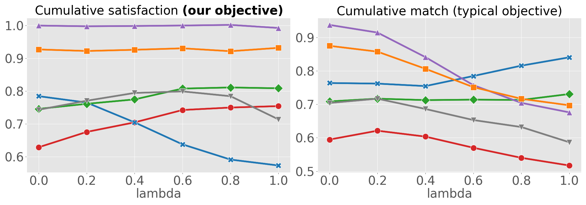
In Figure 2(b), we vary the satisfaction parameter ($\beta$). Since matches that exceed the value of $\beta$ do not lead to the arm’s satisfaction, when this value is small, there arises a significant difference between maximizing matches and maximizing satisfaction. The results show that CAB-UCB provides nearly the same performance as the optimal algorithm in terms of cumulative satisfaction with various satisfaction parameters. It is reasonable that Max match gradually increases cumulative satisfaction as $\beta$ increases. This is because maximizing cumulative matches becomes similar to maximizing cumulative satisfaction when $\beta$ is large. Moreover, CAB-UCB improves satisfaction compared to FairX, which is consistent with the result of Figure 2(a). In terms of matches, we observe that CAB-UCB and CAB-TS ($\theta$) improve cumulative matches as $\beta$ increases, while MaxMatch performs best for smaller values of $\beta$. This is because CAB improves cumulative matches by maximizing cumulative satisfaction when $\beta$ is large.

Figure 2(c) varies the popularity of arms ($\lambda$). The larger value of $\lambda$ represents the situation where all users prefer arms in the same order. We observe that the difference in cumulative satisfaction between CAB-UCB and Max match increases with larger values of $\lambda$. When all users prefer specific arms, Max match mostly selects the most or second most popular arms as shown in Figure 2(d), which reports empirical arm selection probabilities when $\lambda=1.0$ under each method. Moreover, Figure 2(e) reports the average sum of expected matches for selected arms in the last 10 steps, and the black horizontal line indicates the value of $\beta$. It illustrates that Max match chooses the specific arms excessively, assigning more than $\beta$ matches. We can see a similar trend from the results of FairX, although FairX reduces excessive assignments. In contrast, CAB-UCB improves cumulative satisfaction effectively in the situation where Max match, and FairX fail severely, by being aware of the arm satisfaction structure.

6 Conclusions

We proposed CAB, developed its algorithm, established regret upper bounds, and further conducted experimental evaluations of its performance.

We conclude by discussing several directions for future research. One possible direction is to improve the dependence on $\kappa_{\mu}$. An approach toward this improvement is considered in Liu et al. (2025); Zhang et al. (2025). However, instead of assuming Lipschitz continuity with respect to $\mu$, they adopt a different assumption from ours, namely self-concordance. Another natural extension is to consider dynamic environments, in which the set of available arms is not fixed but may evolve, with some arms leaving as a result of the allocation process and new arms emerging. Addressing such settings would require algorithms that can adapt to both statistical uncertainty and changes in the action set.

Appendix A Notations

Table 1 summarizes the symbols used in this paper.

Table 1: Notation

Symbol Meaning $T\in\mathbb{N}$ time horizon $N\in\mathbb{N}$ the number of users $K\in\mathbb{N}$ the number of arms $d\in\mathbb{N}$ dimension of feature vector $\sigma$ parameter about sub-Gaussian $\kappa_{\mu}$ parameter satisfies Assumption 3.1 $\kappa_{r}$ parameter satisfies Assumption D.10 $L_{g}$ Lipschitz constant of function $g$ $D>0$ Upper bound on $\|\theta^{\ast}\|_{2}$ $\mu\colon\mathbb{R}_{\geq 0}\to\mathbb{R}_{\geq 0}$ expectation of feedback $r\colon\mathbb{R}_{\geq 0}\to\mathbb{R}_{\geq 0}$ satifaction function $\phi_{t}(i,a)$ feature vector according to to user $i$ and arm $a$ at round $t$ $x_{t}(i)=\phi_{t}(i,\pi_{t}(i))$ chosen feature vector for user $i$ at round $t$ $y_{t}(i)$ feedback for $i$ at round $t$ $\theta^{\ast}$ unknown parameter $\overline{\theta}_{t}$ MLE of $\theta^{\ast}$ at round $t$ $V_{t}=\sum_{s=1}^{t-1}\sum_{i=1}^{N}x_{s}(i)x_{s}(i)^{\top}+\lambda I$ information matrix at round $t$ $\Pi=\{\pi:[N]\to[K]\}$ set of all functions from $[N]$ to $[K]$ $f_{t}(\pi;\theta)=\sum_{a\in[K]}r(\sum_{i\in\pi^{-1}(a)}\mu(\phi_{t}(i,a)^{\top}\theta))$ cumulative expected satisfaction at round $t$ $\pi_{t}\in\Pi$ chosen allocation at round $t$ $\pi_{t}^{\ast}=\operatorname*{arg\,max}_{\pi\in\Pi}f_{t}(\pi;\theta^{\ast})$ optimal allocation at round $t$ $\mathcal{R}_{T}^{\alpha}=\sum_{t=1}^{T}\left(\alpha f_{t}(\pi_{t}^{\ast};\theta^{\ast})-f_{t}(\pi_{t};\theta^{\ast})\right)$ approximate regret

Appendix B Related Work

We introduce several related works.

Contextual Combinatorial Semi-bandits and Generalized Linear Models

From a technical perspective, a closely related problem setting is that of contextual combinatorial semi-bandits (CCS). CCS was first studied by Qin et al. (2014). CCS are problems in which, at each round, one first observes the arms together with their associated contexts, then selects a combination of arms based on these observations and past outcomes, and finally observes the reward, which depends on the chosen contexts and an unknown parameter. They consider a general framework that includes nonlinear reward functions and propose a UCB algorithm, while assuming a linear model for the feedback. Under CAB with $\mu(x)=x$, their algorithm achieves a regret upper bound of $\widetilde{O}({\max\{\sqrt{d},\sqrt{N}\}}\sqrt{dNT})$. To the best of our knowledge, the best known bound is $\widetilde{O}(d\sqrt{NT}+dN)$, which is achieved by the UCB algorithm of Takemura et al. (2021). In Takemura and Ito (2019), in addition to UCB algorithms, a TS algorithm was studied under the setting where the reward is linear in the feedback, and it was shown that a regret upper bound of $\mathcal{R}_{T}=\widetilde{O}(\max\{d,\sqrt{dN}\}\sqrt{dNT})$ can be achieved. For CCS with linear reward functions, the existing works have investigated lower bounds in addition to upper bounds. In Kveton et al. (2015), a lower bound of $\Omega(\min\{\sqrt{dNT},NT\})$ was established for combinatorial semi-bandits (non-contextual), whereas for CCS, an improved lower bound of $\Omega(\min\{d\sqrt{NT}+dN,NT\})$ was derived by Takemura et al. (2021).

As a related research direction, generalized linear (contextual) bandits have also been studied. In this framework, a generalized linear model is adopted as the feedback model, rather than a linear model, and the contextual bandits setting was first investigated by Filippi et al. (2010). In the non-combinatorial case, existing work on GLM has primarily focused on UCB algorithms (Li et al., 2017; Jun et al., 2017; Lee et al., 2024; Zhang et al., 2025), while TS algorithms have also been developed (Jun et al., 2017; Ding et al., 2021; Kim et al., 2023). On the other hand, to the best of our knowledge, there are only a few studies that consider combinatorial settings. One notable example is Liu et al. (2025), which uses the UCB algorithm and considers a non-contextual setting in which the feedback is sampled from a Bernoulli distribution with its mean specified by a logistic model.

Fair Allocation

One line of research with a closely related idea is fair resource allocation, although the technical relevance is limited. Among them, some studies use an evaluation metric called $\alpha$-fairness, namely $fair_{\alpha}(x)=\frac{x^{1-\alpha}-1}{1-\alpha}$ ($0\geq\alpha<1$). The function $fair_{\alpha}(x)$ is concave, and its use is close in spirit to the idea of this work (Cayci et al., 2020; Si Salem et al., 2022; Sinha et al., 2023). However, they consider an objective function of the form $\sum_{i}fair(\sum_{t=1}^{T}w_{t}(i))$, where $w_{t}(i)$ denotes the utility for $i$ at round $t$, which evaluates the overall fairness across the entire horizon. This differs from our setting. If one emphasizes the final fairness of the allocation over the whole period, their objective function is more appropriate. In contrast, we consider that dissatisfaction over a short period may also lead to churn. Therefore, as an objective function in CAB, we argue that $\sum_{t=1}^{T}f_{t}$ is appropriate.

Moreover, there are technical differences. Representative aspects are the feedback model and the action space. Since the true utility function or the reward vector is observed at the end of each round in their works, their feedback assumption is stronger than the setting we consider (e.g.,the platform observes only whether a match occurred). Regarding the action space, while Sinha et al. (2023, Section 4) discusses integrality constraints, their formulation essentially considers fractional decisions rather than combinatorial ones. Thus, although the high-level idea is similar to our work, the technical setting is entirely different, and a direct comparison of theoretical results is impossible.

Bandits With Fairness Constraints

One line of research addressing fairness in the context of the bandit problem is Joseph et al. (2016). In their work, fairness is defined as allocating arms without favoring any particular arm, based on their expected rewards. On the other hand, a problem that deals with a concept of fairness similar to that considered in this study is the combinatorial sleeping bandits with fairness constraints proposed by Li et al. (2019). In this problem, for each arm $a$, a minimum selection count $n_{a}$ is specified, and the objective is to maximize the cumulative expected reward under this constraint. Li et al. (2019) provided a UCB algorithm, while Huang et al. (2020) later proposed a TS algorithm. Xu et al. (2020) focused on the objective function, considering a setting where the total reward $R$, obtained as a linear combination of the rewards from the arms, is transformed by a strictly concave function $f$, resulting in the objective function $f(R)$. More recently, studies have considered constraints that combine knapsack constraints with fairness constraints (Liu et al., 2022).

Bandits With Knapsacks

The Bandits with Knapsacks (BwK) problem extends the standard bandit setting by introducing knapsack-type resource constraints. Given budget limitations on multiple resources, the learner can no longer obtain rewards once any resource budget is depleted. The goal is to maximize the cumulative expected reward. As a method of introducing constraints into the multi-armed bandits, Badanidiyuru et al. (2013) proposed the BwK framework, which incorporates budget constraints. Building on this framework, subsequent studies have extended the knapsack constraints to linear contextual bandits (Badanidiyuru et al., 2014; Agrawal and Devanur, 2016) and combinatorial semi-bandits (Sankararaman and Slivkins, 2018).

Appendix C NP-hardness

We discuss the computational complexity of this problem and introduce the notion of approximate regret to address it. As the following theorem shows, computing $\pi^{\ast}_{t}$ and $\pi_{t}$ is NP-hard.

Theorem C.1.

Consider a set of $N$ items and $K$ players, and let $r\colon\mathbb{R}\to\mathbb{R}_{\geq 0}$ be a monotone concave function. We consider the problem of maximizing $\sum_{i\in[K]}v_{i}(S_{i})$ subject to $\cup_{i\in[K]}S_{i}=[N]$ and $S_{i}\cap S_{j}=\emptyset$ for $i\neq j$, where $v_{a}\colon 2^{[N]}\to\mathbb{R}{\geq 0}$ is defined by $v_{a}(S)=r\left(\sum_{i\in S}w_{i,a}\right)$, and $w_{i,a}>0$ denotes the value of item $i$ for agent $a$. Then, there exists a concave and monotone increasing function $r$ for which the above problem is NP-hard.

Our proof uses an approach similar to that of Lehmann et al. (2001, Theorem 10).

Proof.

We will perform a reduction from the well-known NP-complete problem ’Knapsack’ (as detailed in Garey and Johnson (1979)). The problem is as follows: given a sequence of integers $a_{1},\dots,a_{m}$ and a target total $t$, the objective is to determine if a subset $S$ of these integers exists such that the sum of the elements in $S$ equals $t$ (i.e., $\sum_{i\in S}a_{i}=t$). Based on this input, we will construct two valuations for the m items.

We consider the decision problem of determining whether $\max f(\mathcal{F})=Vt+V-t$ holds for $\mathcal{F}=\{U_{1},U_{2}\}$ with $U_{1}\cap U_{2}=\emptyset$, $U_{1}\cup U_{2}=U$, $f(\mathcal{F})=v_{1}(U_{1})+v_{2}(U_{2})$, $r(x)=\min\{Vt,x\}$, and $V=\sum_{i\in U}a_{i}$. Let $w_{i,1}=Va_{i},w_{i,2}=a_{i}$. We allocate $S$ to valuation $1$ and $S^{c}$ to valuation $2$. We examine three cases: $\sum_{i\in S}a_{i}=t$, $\sum_{i\in S}a_{i}<t$, and $\sum_{i\in S}a_{i}>t$.

• If $\sum_{i\in S}a_{i}=t$, then $v_{1}(S)+v_{2}(S^{c})=Vt+V-t$.

• If $\sum_{i\in S}a_{i}<t$, then $v_{1}(S)+v_{2}(S^{c})=V\sum_{i\in S}a_{i}+V-\sum_{i\in S}a_{i}<Vt+V-t$.

• If $\sum_{i\in S}a_{i}>t$, then $v_{1}(S)+v_{2}(S^{c})=V\sum_{i\in S}t+V-\sum_{i\in S}a_{i}<Vt+V-t$.

Therefore, the instance of “Knapsack” is a Yes-instance precisely when the proposition is satisfied, and a No-instance otherwise. ∎

Appendix D Details of Section 4

In this section, we provide the omitted proofs in Section 4.

D.1 Technical Lemmas

Here, in preparation for the proofs of the theorems, we introduce technical lemmas that are commonly used in the proofs of Theorems 4.1 and 4.2.

The following lemma guarantees that the estimator $\overline{\theta}_{t}$, obtained by the regularized MLE, “good” estimates the true parameter with high probability. While Kveton et al. (2020, Lemma 9) relies on an initial exploration phase to establish this property, an analogous result can be derived by employing regularization instead.

Lemma D.1.

Assume that $\lambda_{0}\geq\frac{\sigma^{2}}{\kappa_{\mu}^{2}}\left(d\log\left(1+\frac{NT}{d}\right)+2\log\frac{1}{\delta}\right)$. Then, For any $\delta\in(0,1)$, with probability at least $1-\delta$, for all $t\in[T]$,

$$\|\overline{\theta}_{t}-\theta^{\ast}\|_{2}\leq D+1.$$

Proof.

Let $S_{t}=\sum_{s=1}^{t-1}\sum_{i=1}^{N}\big(y_{s}(i)-\mu(x_{s}(i)^{\top}\theta^{\ast})\big)x_{s}(i).$ First, using Chen et al. (1999, Lemma A), we show that the following proposition holds:

$$\|S_{t}-\kappa_{\mu}{\lambda_{0}}\theta^{\ast}\|_{V_{t}^{-1}}\leq\kappa_{\mu}(D+1)\sqrt{{\lambda_{0}}}\Rightarrow\|\overline{\theta}_{t}-\theta^{\ast}\|_{2}\leq D+1.$$

Define the map $H_{t}(\theta)=\sum_{s=1}^{t-1}\sum_{i=1}^{N}\mu(x_{s}(i)^{\top}\theta)x_{s}(i)+\kappa_{\mu}{\lambda_{0}}\theta.$ From the definition of $\overline{\theta}_{t}$, we have $H_{t}(\overline{\theta}_{t})=\sum_{s=1}^{t-1}\sum_{i=1}^{N}y_{s}(i)x_{s}(i).$ Thus, it holds that

$$H_{t}(\overline{\theta}_{t})-H_{t}(\theta^{\ast})=\sum_{s=1}^{t-1}\sum_{i=1}^{N}(y_{s}(i)-\mu(x_{s}(i)^{\top}\theta^{\ast}))x_{s}(i)-\kappa_{\mu}{\lambda_{0}}\theta^{\ast}=S_{t}-\kappa_{\mu}{\lambda_{0}}\theta^{\ast}.$$

Moreover, for any $\theta\in\{\theta\mid\|\theta-\theta^{\ast}\|_{2}\leq D+1\}$, from Assumption 3.1, we have

$$\nabla_{\theta}H_{t}(\theta)=\sum_{s=1}^{t-1}\sum_{i=1}^{N}\dot{\mu}(x_{s}(i)^{\top}\theta)x_{s}(i)x_{s}(i)^{\top}+\kappa_{\mu}{\lambda_{0}}I\succeq\kappa_{\mu}\sum_{s=1}^{t-1}\sum_{i=1}^{N}x_{s}(i)x_{s}(i)^{\top}+\kappa_{\mu}{\lambda_{0}}I=\kappa_{\mu}V_{t}.$$

Therefore, applying Chen et al. (1999, Lemma A) to the map $\theta\mapsto V_{t}^{-1/2}(H_{t}(\theta)-H_{t}(\theta^{\ast}))$ yields the proposition

$$\|S_{t}-\kappa_{\mu}{\lambda_{0}}\theta^{\ast}\|_{V_{t}^{-1}}\leq\kappa_{\mu}(D+1)\sqrt{\lambda_{\min}(V_{t})}\Rightarrow\|\overline{\theta}_{t}-\theta^{\ast}\|_{2}\leq D+1.$$

Since $\lambda_{\min}(V_{t})\geq{\lambda_{0}}$, we obtain

$$\|S_{t}-\kappa_{\mu}{\lambda_{0}}\theta^{\ast}\|_{V_{t}^{-1}}\leq\kappa_{\mu}(D+1)\sqrt{{\lambda_{0}}}\Rightarrow\|\overline{\theta}_{t}-\theta^{\ast}\|_{2}\leq D+1.$$

Next, we upper bound $\|S_{t}-\kappa_{\mu}{\lambda_{0}}\theta^{\ast}\|_{V_{t}^{-1}}$. By the triangle inequality and $V_{t}\succeq{\lambda_{0}}I$, we have

$$\|S_{t}-\kappa_{\mu}{\lambda_{0}}\theta^{\ast}\|_{V_{t}^{-1}}\leq\|S_{t}\|_{V_{t}^{-1}}+\kappa_{\mu}{\lambda_{0}}\|\theta^{\ast}\|_{V_{t}^{-1}}\leq\|S_{t}\|_{V_{t}^{-1}}+\kappa_{\mu}\sqrt{{\lambda_{0}}}\|\theta^{\ast}\|_{2}\leq\|S_{t}\|_{V_{t}^{-1}}+\kappa_{\mu}D\sqrt{{\lambda_{0}}},$$

where the last inequality follows from $\|\theta^{\ast}\|_{2}\leq D$. Thus, we have

$$\|S_{t}\|_{V_{t}^{-1}}\leq\kappa_{\mu}\sqrt{{\lambda_{0}}}\Rightarrow\|\overline{\theta}_{t}-\theta^{\ast}\|_{2}\leq D+1.$$ (7)

Here, from Abbasi-yadkori et al. (2011, Theorem 1), with probability at least $1-\delta$, for all $t\geq 1$, it holds that

$$\|S_{t}\|_{V_{t}^{-1}}^{2}\leq 2\sigma^{2}\log\left(\frac{\det(V_{t})^{1/2}\det\left(\lambda_{0}I\right)^{-1/2}}{\delta}\right)\leq\sigma^{2}d\left(\log\left(1+\frac{Nt}{d\lambda_{0}}\right)+2\log\frac{1}{\delta}\right),$$ (8)

where the second inequality follows from $\det(V_{t})\leq((\operatorname*{tr}(\lambda_{0}I)+Nt)/d)^{d}=(\lambda_{0}+Nt/d)^{d}$. Thus, using (8) and the definiton of $\lambda_{0}$, it holds that $\|S_{t}\|_{V_{t}^{-1}}\leq\kappa_{\mu}\sqrt{{\lambda_{0}}}.$ Therefore, by (7), we have $\|\overline{\theta}_{t}-\theta^{\ast}\|_{2}\leq D+1$ for any $t$ with probability at least $1-\delta$. ∎

The following lemma shows that the regularized MLE also controls the error of the objective function.

Lemma D.2.

Assume that it holds that $\|\overline{\theta}_{t}-\theta^{\ast}\|_{2}\leq D+1$. Then, For any $\delta\in(0,1)$, with probability at least $1-\delta$, for all $t\in[T]$,

$$\lvert f_{t}(\pi;\theta^{\ast})-f_{t}(\pi;\overline{\theta}_{t})\rvert\leq c_{1}\sum_{i=1}^{N}\|\phi_{t}(i,\pi(i))\|_{V_{t}^{-1}},$$

where $c_{1}=\kappa_{\mu}^{-1}L_{r}L_{\mu}\left(\sigma\sqrt{d\log\left(1+\frac{NT}{d\lambda_{0}}\right)+2\log\frac{1}{\delta}}+\kappa_{\mu}D\sqrt{\lambda_{0}}\right)$.

Proof.

Let $S_{t}=\sum_{s=1}^{t-1}\sum_{i=1}^{N}(y_{s}(i)-\mu(x_{s}(i)^{\top}\theta^{\ast}))x_{s}(i)$, $\mathcal{D}_{1}=\{x_{s}(i),y_{s}(i)\}_{i\in[N],s<t}$, and $\mathcal{D}_{2}=\{x_{s}(i),\mu(x_{s}(i)^{\top}\theta^{\ast})\}_{i\in[N],s<t}$.

First, we expand Kveton et al. (2020, Lemma 1) to the regularized MLE. It holds that

$$S_{t} =\nabla_{\theta}\mathcal{L}(D_{2};\theta^{\ast})-\nabla_{\theta}\mathcal{L}(D_{1};\theta^{\ast})=\nabla_{\theta}\widetilde{\mathcal{L}}(D_{1};\overline{\theta}_{t},\kappa_{\mu}\lambda_{0})-\nabla_{\theta}\mathcal{L}(D_{1};\theta^{\ast})$$

$$=\nabla_{\theta}\widetilde{\mathcal{L}}(D_{1};\overline{\theta}_{t},\kappa_{\mu}\lambda_{0})-\nabla_{\theta}\widetilde{\mathcal{L}}(D_{1};\theta^{\ast},\kappa_{\mu}\lambda_{0})+\kappa_{\mu}\lambda_{0}\theta^{\ast}=\nabla_{\theta}^{2}\widetilde{\mathcal{L}}(D_{1};\theta^{\prime},\kappa_{\mu}\lambda_{0})(\overline{\theta}_{t}-\theta^{\ast})+\kappa_{\mu}\lambda_{0}\theta^{\ast}$$

$$=V(\overline{\theta}_{t}-\theta^{\ast})+\kappa_{\mu}\lambda_{0}\theta^{\ast},$$

where $\theta^{\prime}$ is a convex combination of $\overline{\theta}_{t}$ and $\theta^{\ast}$, and $V=\nabla_{\theta}^{2}\widetilde{\mathcal{L}}(D_{1};\theta^{\prime},\kappa_{\mu}\lambda_{0})$. We used $\nabla_{\theta}\mathcal{L}(D_{2};\theta^{\ast})=\nabla_{\theta}\widetilde{\mathcal{L}}(D_{1};\overline{\theta}_{t},\kappa_{\mu}\lambda_{0})=0$ in the second equality.

Next, we bound $\lvert f_{t}(\pi;\theta^{\ast})-f_{t}(\pi;\overline{\theta}_{t})\rvert$.

$$\lvert f_{t}(\pi;\theta^{\ast})-f_{t}(\pi;\overline{\theta}_{t})\rvert \leq L_{r}L_{\mu}\sum_{i=1}^{N}\lvert x_{t}(i)^{\top}(\theta^{\ast}-\overline{\theta}_{t})\rvert$$

$$\leq L_{r}L_{\mu}\sum_{i=1}^{N}\|x_{t}(i)\|_{V_{t}^{-1}}\|\theta^{\ast}-\overline{\theta}_{t}\|_{V_{t}}=L_{r}L_{\mu}\sum_{i=1}^{N}\|x_{t}(i)\|_{V_{t}^{-1}}\|V^{-1}S_{t}-\kappa_{\mu}\lambda_{0}V^{-1}\theta^{\ast}\|_{V_{t}}$$

$$\leq L_{r}L_{\mu}\sum_{i=1}^{N}\|x_{t}(i)\|_{V_{t}^{-1}}(\|V^{-1}S_{t}\|_{V_{t}}+\kappa_{\mu}\lambda_{0}\|V^{-1}\theta^{\ast}\|_{V_{t}})$$

$$\leq L_{r}L_{\mu}\sum_{i=1}^{N}\|x_{t}(i)\|_{V_{t}^{-1}}(\sqrt{S_{t}^{\top}V^{-1}V_{t}V^{-1}S_{t}}+\kappa_{\mu}\lambda_{0}\sqrt{\theta^{\ast\top}V^{-1}V_{t}V^{-1}\theta^{\ast}})$$

$$\leq\kappa_{\mu}^{-1}L_{r}L_{\mu}\sum_{i=1}^{N}\|x_{t}(i)\|_{V_{t}^{-1}}(\|S_{t}\|_{V_{t}^{-1}}+\kappa_{\mu}D\sqrt{\lambda_{0}}),$$

where the second inequality follows from the Cauchy-Schwarz inequality, and the last inequality follows from the $\kappa_{\mu}V_{t}\preceq V$ on $\|\overline{\theta}_{t}-\theta^{\ast}\|_{2}\leq D+1$.

Therefore, combining the above ineqaulity with (8) in the proof of Lemma D.1, we have that, with probability at least $1-\delta$, for all $t\geq 1$,

$$\lvert f_{t}(\pi;\theta^{\ast})-f_{t}(\pi;\overline{\theta}_{t})\rvert\leq\kappa_{\mu}^{-1}L_{r}L_{\mu}\left(\sigma\sqrt{d\log\left(1+\frac{Nt}{d\lambda_{0}}\right)+2\log\frac{1}{\delta}}+\kappa_{\mu}D\sqrt{\lambda_{0}}\right)\sum_{i=1}^{N}\|x_{t}(i)\|_{V_{t}^{-1}}.$$

∎

We can bound $\sum_{t=1}^{T}\sum_{i=1}^{N}\|x_{t}(i)\|_{V_{t}^{-1}}^{2}$ using the following lemma:

Lemma D.3 (Takemura et al. 2021, Lemma 2).

Let $\{x_{t}(i)\}_{(i,t)\in[N]\times\mathbb{N}}$ a sequence in $\mathbb{R}^{d}$ satisfying $\|x_{t}(i)\|_{2}\leq 1$. For all $t\geq 1$, define $V_{t}=\lambda_{0}I+\sum_{s=1}^{t-1}\sum_{i=1}^{N}x_{s}(i)x_{s}(i)^{\top}$, where $\lambda_{0}\geq 0$. It holds that

$$\sum_{t=1}^{T}\sum_{i=1}^{N}\min\left\{\frac{1}{\sqrt{N}},\|x_{t}(i)\|_{V_{t}^{-1}}\right\} \leq\sqrt{2dNT\log\left(1+\frac{NT}{d\lambda_{0}}\right)},\quad\text{and}$$

$$\sum_{t=1}^{T}\sum_{i=1}^{N}\mathds{1}\left[\|x_{t}(i)\|_{V_{t}^{-1}}>\frac{1}{\sqrt{N}}\right] <2dN\log\left(1+\frac{NT}{d\lambda_{0}}\right).$$

This lemma implies that

$$\sum_{t=1}^{T}\sum_{i=1}^{N}\|x_{t}(i)\|_{V_{t}^{-1}} =\sum_{t=1}^{T}\sum_{i=1}^{N}\left(\mathds{1}\left[\|x_{t}(i)\|_{V_{t}^{-1}}>\frac{1}{\sqrt{N}}\right]+\mathds{1}\left[\|x_{t}(i)\|_{V_{t}^{-1}}\leq\frac{1}{\sqrt{N}}\right]\right)\|x_{t}(i)\|_{V_{t}^{-1}}$$

$$\leq\sqrt{2dNT\log\left(1+\frac{NT}{d\lambda_{0}}\right)}+\frac{2dN}{\sqrt{\lambda_{0}}}\log\left(1+\frac{NT}{d\lambda_{0}}\right)$$ (9)

D.2 Details of Section 4.1

We provide the complete version of Theorem 4.1.

Theorem D.4.

Fix any $\delta\in(0,1)$. If we run Algorithm 1 with $c_{1}=\frac{L_{r}L_{\mu}}{\kappa_{\mu}}\big(\sigma\sqrt{d\log\left(1+\frac{Nt}{d\lambda_{0}}\right)+2\log\frac{1}{\delta}}+\kappa_{\mu}D\sqrt{\lambda_{0}}\big)$ and $\lambda_{0}\geq\frac{\sigma^{2}}{\kappa_{\mu}^{2}}\left(d\log\left(1+\frac{NT}{d}\right)+2\log\frac{1}{\delta}\right)$, then, with probability at least $1-2\delta$, the regret of algorithm is upper bounded by

$$\mathcal{R}_{T}^{\alpha} \leq 2c_{1}\left(\sqrt{2dNT\log\left(1+\frac{NT}{d\lambda_{0}}\right)}+\frac{2dN}{\sqrt{\lambda_{0}}}\log\left(1+\frac{NT}{d\lambda_{0}}\right)\right).$$

If we set $\lambda_{0}=\kappa_{\mu}^{-2}\sigma^{2}\left(d\log\left(1+\frac{NT}{d}\right)+2\log\frac{1}{\delta}\right)$, we have

$$\mathcal{R}_{T}=\widetilde{O}(d\sqrt{NT}+dN).$$

Proof.

We define $x_{t}^{\ast}(i)=\phi_{t}(i,\pi_{t}^{\ast}(i))$, $\Delta_{t}=\overline{\theta}_{t}-\theta^{\ast}$. First, we bound the one-step regret, $f_{t}(\pi_{t}^{\ast};\theta^{\ast})-f_{t}(\pi_{t};\theta^{\ast})$, for fixed $t>\tau$. Here, we want to bound the following terms:

$$\alpha f_{t}(\pi_{t}^{\ast};\theta^{\ast})-f_{t}(\pi_{t};\theta^{\ast})=(\alpha f_{t}(\pi_{t}^{\ast};\overline{\theta}_{t})-f_{t}(\pi_{t};\overline{\theta}_{t}))+\alpha(f_{t}(\pi_{t}^{\ast};\theta^{\ast})-f_{t}(\pi_{t}^{\ast};\overline{\theta}_{t}))+(f_{t}(\pi_{t};\overline{\theta}_{t})-f_{t}(\pi_{t};\theta^{\ast})).$$

From the definition of $\pi_{t},$ the first term is bounded as

$$\alpha f_{t}(\pi_{t}^{\ast};\overline{\theta}_{t})-f_{t}(\pi_{t};\overline{\theta}_{t})\leq g_{t}(\pi_{t})-\alpha g_{t}(\pi_{t}^{\ast})=c_{1}\sum_{i=1}^{N}(\|x_{t}(i)\|_{V_{t}^{-1}}-\alpha\|x_{t}^{\ast}(i)\|_{V_{t}^{-1}}).$$ (10)

The second and third term is bounded as

$$\alpha(f_{t}(\pi_{t}^{\ast};\theta^{\ast})-f_{t}(\pi_{t}^{\ast};\overline{\theta}_{t})) \leq\alpha c_{1}\sum_{i=1}^{N}\|x_{t}^{\ast}(i)\|_{V_{t}^{-1}},$$ (11)

$$f_{t}(\pi_{t};\overline{\theta}_{t})-f_{t}(\pi_{t};\theta^{\ast}) \leq c_{1}\sum_{i=1}^{N}\|x_{t}(i)\|_{V_{t}^{-1}}$$ (12)

from Lemma D.2.

Combining (10), (11), and (12), with probability at least $1-2\delta$, it holds that

$$f_{t}(\pi_{t}^{\ast};\theta^{\ast})-f_{t}(\pi_{t};\theta^{\ast})\leq 2c_{1}\sum_{i=1}^{N}\|x_{t}(i)\|_{V_{t}^{-1}}.$$

Since $\|x_{t}(i)\|_{2}\leq 1$, we have

$$\sum_{t=1}^{T}(f_{t}(\pi_{t}^{\ast};\theta^{\ast})-f_{t}(\pi_{t};\theta^{\ast})) \leq 2c_{1}\sum_{t=1}^{T}\sum_{i=1}^{N}\|x_{t}(i)\|_{V_{t}^{-1}}\leq 2c_{1}\sqrt{NT}\sqrt{\sum_{t=1}^{T}\sum_{i=1}^{N}\|x_{t}(i)\|^{2}_{V_{t}^{-1}}}$$

$$\leq 2c_{1}\left(\sqrt{2dNT\log\left(1+\frac{NT}{d\lambda_{0}}\right)}+\frac{2dN}{\sqrt{\lambda_{0}}}\log\left(1+\frac{NT}{d\lambda_{0}}\right)\right),$$ (13)

where the second inequality follows from the Cauchy–Schwartz inequality and the last inequality follows from Section D.1. This is the desired upper bound. ∎

D.3 Details of Section 4.2.1

Here is the complete version of Theorem 4.2.

Theorem D.5.

Algorithm 2 with $a=c_{1}\sqrt{L_{\mu}N}$ and $\lambda_{0}\geq\kappa_{\mu}^{-2}\sigma^{2}\left(d\log\left(1+\frac{NT}{d}\right)+2\log\frac{1}{\delta}\right)$ achieves the following regret bound for any $\delta\in(0,1/T)$:

$$\mathbb{E}[\mathcal{R}_{T}^{\alpha}] \leq(c_{1}+c_{2})\left(1+\frac{2}{0.15-2\delta}\right)\left(\sqrt{2dNT\log\left(1+\frac{NT}{d\lambda_{0}}\right)}+\frac{2dN}{\sqrt{\lambda_{0}}}\log\left(1+\frac{NT}{d\lambda_{0}}\right)\right)+4\delta MT,$$

where $c_{1}=\kappa_{\mu}^{-1}L_{r}L_{\mu}\left(\sigma\sqrt{d\log\left(1+\frac{Nt}{d\lambda_{0}}\right)+2\log\frac{1}{\delta}}+\kappa_{\mu}D\sqrt{\lambda_{0}}\right)$ and $c_{2}=c_{1}\sqrt{2\kappa_{\mu}^{-1}L_{\mu}N\log\frac{KN}{\delta}}$.

If we set $\lambda_{0}=\kappa_{\mu}^{-2}\sigma^{2}\left(d\log\left(1+\frac{NT}{d}\right)+2\log\frac{1}{\delta}\right)$, we have

$$\mathcal{R}_{T}=\widetilde{O}(dN\sqrt{T}+dN^{3/2}).$$

To prove Theorem D.5, we first bound the one-step regret. For convenience, we define

$$E_{1,t}=\{{}^{\forall}\pi\in\Pi\mid\lvert f_{t}(\pi;\theta^{\ast})-f_{t}(\pi;\overline{\theta}_{t})\rvert\leq c_{1}\sum_{i=1}^{N}\|\phi_{t}(i,\pi(i))\|_{V_{t}^{-1}}\}.$$ (14)

Lemma D.6.

Define events $E_{2,t}$ and $E_{3,t}$ as

$$E_{2,t} =\left\{{}^{\forall}\pi\in\Pi\mid\lvert h_{t}(\pi;\widetilde{\bm{\varepsilon}}_{t})\rvert\leq c_{2}\sum_{i=1}^{N}\|\phi_{t}(i,\pi(i))\|_{V_{t}^{-1}}\right\},\>\>\text{and}$$

$$E_{3,t} =\left\{h_{t}(\pi_{t}^{\ast};\widetilde{\bm{\varepsilon}}_{t})>c_{1}\sum_{i=1}^{N}\|\phi_{t}(i,\pi_{t}^{\ast}(i))\|_{V_{t}^{-1}}\right\}.$$

Let $\mathbb{P}_{t}(E_{2,t})\geq 1-p_{2}$ and $\mathbb{P}_{t}(E_{3,t})\geq p_{3}$ ($p_{3}>p_{2}$). If $E_{1,t}$ holds, then we have

$$\mathbb{E}_{t}[\alpha f_{t}(\pi_{t}^{\ast};\theta^{\ast})-f_{t}(\pi_{t};\theta^{\ast})]\leq(c_{1}+c_{2})\left(1+\frac{2\alpha}{p_{3}-p_{2}}\right)\mathbb{E}_{t}\left[\sum_{i=1}^{N}\|x_{t}(i)\|_{V_{t}^{-1}}\right]+p_{2}M$$

Proof.

Let $c=c_{1}+c_{2}$, $\mathcal{S}_{t}=\{\pi\in\Pi\mid c\sum_{i=1}^{N}\|x_{t}(i)\|_{V_{t}^{-1}}<f_{t}(\pi_{t}^{\ast};\theta^{\ast})-f_{t}(\pi;\theta^{\ast})\}$, $\overline{\mathcal{S}}_{t}=\mathcal{A}_{t}/\mathcal{S}_{t}$, and $\pi_{t}^{\prime}=\operatorname*{arg\,min}_{\pi\in\overline{\mathcal{S}}_{t}}\sum_{i=1}^{N}\|\phi_{t}(i,\pi(i))\|_{V_{t}^{-1}}$.

First, we will bound $\alpha f_{t}(\pi_{t}^{\ast};\theta^{\ast})-f_{t}(\pi_{t};\theta^{\ast})$ on $E_{2,t}$. At round $t$ on $E_{2,t}$, we have

$$f_{t}(\pi_{t}^{\ast};\theta^{\ast})-f_{t}(\pi_{t};\theta^{\ast}) \leq f_{t}(\pi_{t}^{\ast};\theta^{\ast})-f_{t}(\pi_{t}^{\prime};\theta^{\ast})+(f_{t}(\pi_{t}^{\prime};\overline{\theta}_{t})+h_{t}(\pi_{t}^{\prime};\widetilde{\bm{\varepsilon}}_{t}))-(f_{t}(\pi_{t};\overline{\theta}_{t})+h_{t}(\pi_{t};\widetilde{\bm{\varepsilon}}_{t}))$$

$$\quad+h_{t}(\pi_{t};\widetilde{\bm{\varepsilon}}_{t})-h_{t}(\pi_{t}^{\prime};\widetilde{\bm{\varepsilon}}_{t})+c_{1}\sum_{i=1}^{N}(\|\phi_{t}(i,\pi_{t}^{\prime}(i))\|_{V_{t}^{-1}}+\|\phi_{t}(i,\pi_{t}(i))\|_{V_{t}^{-1}})$$

$$\leq(c_{1}+c_{2})\sum_{i=1}^{N}(2\|\phi_{t}(i,\pi_{t}^{\prime}(i))\|_{V_{t}^{-1}}+\|\phi_{t}(i,\pi_{t}(i))\|_{V_{t}^{-1}}),$$

where the first inequality follows from the definition of $E_{1,t}$ and $E_{2,t}$, and the second inequality follows from the property of $\alpha$-approximation oracle, and the definition of $\mathcal{S}_{t}$ and $\pi_{t}^{\prime}$.

Second, we want to bound $\mathbb{E}_{t}\left[\sum_{i=1}^{N}\|\phi_{t}(i,\pi_{t}^{\prime}(i))\|_{V_{t}^{-1}}\right]$ by $\mathbb{E}_{t}\left[\sum_{i=1}^{N}\|\phi_{t}(i,\pi_{t}(i))\|_{V_{t}^{-1}}\right]$. Note that

$$\mathbb{E}_{t}[\sum_{i=1}^{N}\|\phi_{t}(i,\pi_{t}(i))\|_{V_{t}^{-1}}] \geq\mathbb{E}_{t}[\sum_{i=1}^{N}\|\phi_{t}(i,\pi_{t}^{\prime}(i))\|_{V_{t}^{-1}}\mid\pi_{t}\in\overline{\mathcal{S}}_{t}]\mathbb{P}_{t}(\pi_{t}\in\overline{\mathcal{S}}_{t})$$

$$\geq\sum_{i=1}^{N}\|\phi_{t}(i,\pi_{t}^{\prime}(i))\|_{V_{t}^{-1}}\mathbb{P}_{t}(\pi_{t}\in\overline{\mathcal{S}}_{t}).$$

Thus, $\mathbb{E}_{t}[f_{t}(\pi_{t}^{\ast};\theta^{\ast})-f_{t}(\pi_{t};\theta^{\ast})]\leq c(1+2/\mathbb{P}_{t}(\pi_{t}\in\overline{\mathcal{S}}_{t}))\sum_{i=1}^{N}\|\phi_{t}(i,\pi_{t}(i))\|_{V_{t}^{-1}}$ on $E_{2,t}$.

Third, we will lower-bound $\mathbb{P}_{t}(\pi_{t}\in\overline{\mathcal{S}}_{t})$.

$$\mathbb{P}_{t}(\pi_{t}\in\overline{\mathcal{S}}_{t}) \geq\mathbb{P}_{t}\left({}^{\exists}\pi\in\overline{\mathcal{S}}_{t},f_{t}(\pi;\overline{\theta}_{t})+h_{t}(\pi;\widetilde{\bm{\varepsilon}}_{t})>\max_{\pi^{\prime}\in\mathcal{S}_{t}}f_{t}(\pi^{\prime};\overline{\theta}_{t})+h_{t}(\pi^{\prime};\widetilde{\bm{\varepsilon}}_{t})\right)$$

$$\geq\mathbb{P}_{t}\left(f_{t}(\pi_{t}^{\ast};\overline{\theta}_{t})+h_{t}(\pi_{t}^{\ast};\widetilde{\bm{\varepsilon}}_{t})>\max_{\pi^{\prime}\in\mathcal{S}_{t}}f_{t}(\pi^{\prime};\overline{\theta}_{t})+h_{t}(\pi^{\prime};\widetilde{\bm{\varepsilon}}_{t})\right)$$

$$\geq\mathbb{P}_{t}\left(f_{t}(\pi_{t}^{\ast};\overline{\theta}_{t})+h_{t}(\pi_{t}^{\ast};\widetilde{\bm{\varepsilon}}_{t})>f_{t}(\pi_{t}^{\ast};\theta^{\ast}),E_{2,t}\right)$$

$$\geq\mathbb{P}_{t}\left(f_{t}(\pi_{t}^{\ast};\overline{\theta}_{t})+h_{t}(\pi_{t}^{\ast};\widetilde{\bm{\varepsilon}}_{t})>f_{t}(\pi_{t}^{\ast};\overline{\theta}_{t})+c_{1}\sum_{i=1}^{N}\|\phi_{t}(i,\pi_{t}^{\ast}(i))\|_{V_{t}^{-1}}\right)-\mathbb{P}\left(\overline{E}_{2,t}\right)$$

$$\geq\mathbb{P}_{t}\left(h_{t}(\pi_{t}^{\ast};\widetilde{\bm{\varepsilon}}_{t})>c_{1}\sum_{i=1}^{N}\|\phi_{t}(i,\pi_{t}^{\ast}(i))\|_{V_{t}^{-1}}\right)-\mathbb{P}\left(\overline{E}_{2,t}\right),$$

where the first inequality follows from the definition of $\overline{\mathcal{S}}_{t}$, the second inequality follows from the fact that $A_{t}^{\ast}\in\overline{\mathcal{S}}_{t}$, the forth inequality follows from $f_{t}(\pi;\overline{\theta}_{t})+h_{t}(\pi;\widetilde{\bm{\varepsilon}}_{t})\leq f_{t}(\pi;\theta^{\ast})+(c_{1}+c_{2})\sum_{i=1}^{N}\|\phi_{t}(i,\pi(i))\|_{V_{t}^{-1}}\leq f_{t}(\pi_{t}^{\ast};\theta^{\ast})$ for any $\pi\in\mathcal{S}_{t}$ on $E_{1,t}$ and $E_{2,t}$, and the last inequality follows from the definition of $E_{1,t}$.

Finally, we can achieve the desired bound, using the inequality,

$$\mathbb{E}_{t}[f_{t}(\pi_{t}^{\ast};\theta^{\ast})-f_{t}(\pi_{t};\theta^{\ast})] =\mathbb{E}_{t}[(f_{t}(\pi_{t}^{\ast};\theta^{\ast})-f_{t}(\pi_{t};\theta^{\ast}))\mathds{1}[E_{2,t}]]+\mathbb{E}_{t}[(f_{t}(\pi_{t}^{\ast};\theta^{\ast})-f_{t}(\pi_{t};\theta^{\ast}))\mathds{1}[\overline{E}_{2,t}]]$$

$$\leq\mathbb{E}_{t}[(f_{t}(\pi_{t}^{\ast};\theta^{\ast})-f_{t}(\pi_{t};\theta^{\ast}))\mathds{1}[E_{2,t}]]+M\mathbb{P}_{t}(\overline{E}_{2,t}).$$

∎

$p_{2}$ and $p_{3}$ in Lemma D.6 can be bounded as follows, respectively.

Lemma D.7.

For each $t\geq 1$, $E_{2,t}$ holds with probability at least $1-2\delta$.

Lemma D.8.

$E_{3,t}$ holds with probability at least $0.15$.

We prove these lemmas.

Proof of Lemma D.7.

From Kveton et al. (2020, Lemma 4), $E_{2,t}^{\prime}=\{{}^{\forall}(i,a)\in[N]\times[K]\mid\lvert\phi_{t}(i,a)^{\top}\widetilde{\varepsilon}_{t}(i)\rvert\leq c_{2}\|\phi_{t}(i,a)\|_{V_{t}^{-1}}\}$ holds with probability at least $1-2\delta$. Their proof uses the union bound, so we can apply that lemma to our algorithm, which samples $\widetilde{\varepsilon}_{t}(i)$ independently for each $i\in[N]$. On $E_{2,t}^{\prime}$, we have $\sum_{i=1}^{N}\lvert\phi_{t}(i,\pi(i))^{\top}\widetilde{\varepsilon}_{t}(i)\rvert\leq c_{2}\sum_{i=1}^{N}\|\phi_{t}(i,\pi(i))\|_{V_{t}^{-1}}$ for any $\pi\in\Pi$. In addition, we have $\lvert h_{t}(\pi;\widetilde{\bm{\varepsilon}}_{t})\rvert\leq\sum_{i=1}^{N}\lvert\phi_{t}(i,\pi(i))^{\top}{\widetilde{\varepsilon}_{t}(i)}\rvert$ from the triangle inequality. Theorefore, on $E_{2,t}^{\prime}$, it holds that $\lvert h_{t}(\pi;\widetilde{\bm{\varepsilon}}_{t})\rvert\leq c_{2}\sum_{i=1}^{N}\|\phi_{t}(i,\pi(i))\|_{V_{t}^{-1}}$ for any $\pi\in\Pi$. In other words, $E_{2,t}$ holds with probability at least $1-2\delta$. ∎

Proof of Lemma D.8.

Using $H_{t}\preceq L_{\mu}V_{t}$, and Cauchy–Schwarz inequality, we have

$$\mathbb{P}_{t}\left(h_{t}(\pi_{t}^{\ast};\widetilde{\bm{\varepsilon}}_{t})>c_{1}\sum_{i=1}^{N}\|\phi_{t}(i,\pi_{t}^{\ast}(i))\|_{V_{t}^{-1}}\right) \geq\mathbb{P}_{t}\left(h_{t}(\pi_{t}^{\ast};\widetilde{\bm{\varepsilon}}_{t})>c_{1}\sqrt{L_{\mu}N\sum_{i=1}^{N}\|\phi_{t}(i,\pi_{t}^{\ast}(i))\|_{H_{t}^{-1}}^{2}}\right)$$

$$=\mathbb{P}_{t}\left(\sum_{i=1}^{N}\phi_{t}(i,\pi_{t}^{\ast}(i))^{\top}\widetilde{\varepsilon}_{t}(i)>a\sqrt{\sum_{i=1}^{N}\|\phi_{t}(i,\pi_{t}^{\ast}(i))\|_{H_{t}^{-1}}^{2}}\right)$$ (15)

Next, we derive a lower bound. From $\widetilde{\varepsilon}_{t}(i)\sim\mathcal{N}(\bm{0},a^{2}H_{t}^{-1})$, we have $\phi_{t}(i,\pi_{t}^{\ast}(i))^{\top}\widetilde{\varepsilon}_{t}(i)\sim\mathcal{N}(0,a^{2}\|\phi_{t}(i,\pi_{t}^{\ast}(i))\|_{H_{t}^{-1}}^{2})$. Moreover, since $\{\widetilde{\varepsilon}_{t}(i)\}_{i=1}^{N}$ are independent, it follows that $\sum_{i=1}^{N}\phi_{t}(i,\pi_{t}^{\ast}(i))^{\top}\widetilde{\varepsilon}_{t}(i)\sim\mathcal{N}(0,a^{2}\sum_{i=1}^{N}\|\phi_{t}(i,\pi_{t}^{\ast}(i))\|_{H_{t}^{-1}}^{2})$. Consequently, we obtain

$$\mathbb{P}_{t}\left(\sum_{i=1}^{N}\phi_{t}(i,\pi_{t}^{\ast}(i))^{\top}\widetilde{\varepsilon}_{t}(i)>a\sqrt{\sum_{i=1}^{N}\|\phi_{t}(i,\pi_{t}^{\ast}(i))\|_{H_{t}^{-1}}^{2}}\right)\geq 0.15.$$ (16)

Combining (D.3) with (16) yields the desired bound. ∎

We are now ready to prove Theorem D.5.

Proof of Theorem D.5.

Let $E_{4,t}=\{\|\overline{\theta}_{t}-\theta^{\ast}\|_{2}\leq D+1\}$, $\mathbb{P}(E_{4,t})\geq 1-p_{4}$, $p_{1}\geq\mathbb{P}(\overline{E}_{1,t}\land E_{4,t})$, $\mathbb{P}_{t}(\overline{E}_{2,t})\geq 1-p_{2}$ on the event $E_{4,t}$, and $\mathbb{P}_{t}(E_{3,t})\geq 1-p_{3}$.

$$\mathbb{E}[\mathcal{R}_{T}^{\alpha}] =\sum_{t=1}^{T}\mathbb{E}[f_{t}(\pi_{t}^{\ast};\theta^{\ast})-f_{t}(\pi_{t};\theta^{\ast})]$$

$$\leq\sum_{t=1}^{T}\mathbb{E}[(f_{t}(\pi_{t}^{\ast};\theta^{\ast})-f_{t}(\pi_{t};\theta^{\ast}))\mathds{1}[E_{1,t},E_{4,t}]]+(p_{1}+p_{4})MT$$

$$\leq\sum_{t=1}^{T}\mathbb{E}[\mathbb{E}_{t}[(f_{t}(\pi_{t}^{\ast};\theta^{\ast})-f_{t}(\pi_{t};\theta^{\ast}))\mathds{1}[E_{1,t},E_{4,t}]]]+(p_{1}+p_{4})MT$$

From Lemma D.6, it holds that

$$\mathbb{E}[\mathcal{R}_{T}^{\alpha}] \leq(c_{1}+c_{2})\left(1+\frac{2}{p_{3}-p_{2}}\right)\mathbb{E}\left[\sum_{t=1}^{T}\sum_{i=1}^{N}\|x_{t}(i)\|_{V_{t}^{-1}}\right]+(p_{1}+p_{2}+p_{4})MT$$

$$\leq(c_{1}+c_{2})\left(1+\frac{2}{p_{3}-p_{2}}\right)\mathbb{E}\left[\sqrt{NT\sum_{t=1}^{T}\sum_{i=1}^{N}\|x_{t}(i)\|_{V_{t}^{-1}}^{2}}\right]+(p_{1}+p_{2}+p_{4})MT,$$

where we used the Cauchy-Schwarz inequality in the last inequality.

Next, we bound $p_{1}$, $p_{2}$, $p_{3}$, and $p_{4}$. From Lemmas D.2, D.7, D.8 and D.1, we have $p_{1}\leq\delta$, $p_{2}\leq 2\delta$, $p_{3}\geq 0.15$, and $p_{4}\leq\delta$. In addition, from the definition of $\lambda_{0}$, we have $p_{4}\leq\delta$ from Kveton et al. (2020, Lemma 9). Therefore, using these bounds and Section D.1, we can achieve the desired bound. ∎

Remark D.9.

For each $i$, sampling i.i.d. from a Gaussian distribution is used to obtain a lower bound for (D.3). Indeed, $\sum_{i=1}^{N}\phi_{t}(i,\pi_{t}^{\ast}(i))^{\top}\widetilde{\varepsilon}_{t}(i)\sim\mathcal{N}(0,a^{2}\sum_{i=1}^{N}\|\phi_{t}(i,\pi_{t}^{\ast}(i))\|_{H_{t}^{-1}}^{2})$, which leads to the bound in (16), is derived from the independence. On the other hand, if we sample a single $\overline{\varepsilon}_{t}$ from $\mathcal{N}(0,a^{2}\sum_{i=1}^{N}\|\phi_{t}(i,\pi_{t}^{\ast}(i))\|_{H_{t}^{-1}}^{2})$ and set $\widetilde{\varepsilon}_{t}(i)=\overline{\varepsilon}_{t}$ for any $i\in[N]$, then $\sum_{i=1}^{N}\phi_{t}(i,\pi_{t}^{\ast}(i))^{\top}\widetilde{\varepsilon}_{t}(i)\sim\mathcal{N}(0,a^{2}\|\sum_{i=1}^{N}\phi_{t}(i,\pi_{t}^{\ast}(i))\|_{H_{t}^{-1}}^{2})$, and this prevents us from obtaining a desirable probability bound.

D.4 Variant of Algorithm 2

In this section, we provide a variant of the TS algorithm.

In Algorithm 2, we sample $\widetilde{\varepsilon}_{t}(i)$ from $\mathcal{N}(\bm{0},a^{2}H_{t}^{-1})$ for any $i\in[N]$, and maximize $f_{t}(\pi;\overline{\theta}_{t})+h_{t}(\pi;\widetilde{\bm{\varepsilon}}_{t})$. However, it is also a natural idea to sample $\widetilde{\theta}_{t}(i)$ from $\mathcal{N}(\overline{\theta}_{t},a^{2}H_{t}^{-1})$ and instead maximize $\widetilde{f}_{t}$, defined as follows:

$$\widetilde{f}_{t}(\pi;\bm{\theta})=\sum_{a\in[K]}r\left(\sum_{i\in\pi^{-1}(a)}\mu(\phi_{t}(i,a)^{\top}\theta(i))\right).$$ (17)

The algorithm can be written as Algorithm 3. Note that from a theoretical standpoint, this algorithm has weaknesses compared with Algorithm 2, as discussed in Remark D.15.

Algorithm 3 CAB-TS (variant)

1:The total rounds $T$, the number of users $N$, and tuning parameter $\lambda_{0}$ and $a$.

2:$\mathcal{D}_{0}=\varnothing$

3:for $t=1,\dots,T$ do

4:  $V_{t}\leftarrow\lambda_{0}I+\sum_{s=1}^{t-1}\sum_{i=1}^{N}x_{s}(i)x_{s}(i)^{\top}$.

5:  $\overline{\theta}_{t}\leftarrow\operatorname*{arg\,min}_{\theta\in\mathbb{R}^{d}}\widetilde{\mathcal{L}}(\mathcal{D}_{t};\theta,\kappa_{\mu}\lambda_{0})$.

6:  $H_{t}\leftarrow\sum_{s=1}^{t-1}\sum_{i=1}^{N}\dot{\mu}(x_{s}(i)^{\top}\overline{\theta}_{t})(x_{s}(i)x_{s}(i)^{\top}+\frac{\lambda_{0}}{N(t-1)}I)$.

7:  for $i=1,\dots,N$ do

8:   $\widetilde{\theta}_{t}(i)\overset{\text{i.i.d.}}{\sim}\mathcal{N}(\overline{\theta}_{t},a^{2}H_{t}^{-1})$.   

9:  Choose $\pi_{t}=\operatorname*{arg\,max}_{\pi\in\Pi}\widetilde{f}_{t}(\pi;\widetilde{\bm{\theta}}_{t})$, where $\widetilde{f}_{t}$ is defined in (17).

10:  Observe $y_{t}(i)$ for any $i\in[N]$.

11:  Let $x_{t}(i)\leftarrow\phi_{t}(i,\pi_{t}(i))$ for any $i\in[N]$ and $\mathcal{D}_{t+1}\leftarrow\mathcal{D}_{t}\cup\{(x_{t},(i),y_{t}(i))\}_{i\in[N]}$.

D.4.1 Regret Analysis

In the following part, let

$$c_{1}^{\star} =\kappa_{\mu}^{-1}L_{r}L_{\mu}\left(\sigma\sqrt{d\log\left(1+\frac{Nt}{d\lambda_{0}}\right)+2\log\frac{1}{\delta}}+\kappa_{\mu}D\sqrt{\lambda_{0}}\right),\>\>\text{and}$$

$$c_{2}^{\star} =c_{1}^{\star}\kappa_{r}^{-1}\kappa_{\mu}^{-3/2}L_{r}L_{\mu}^{3/2}\sqrt{2N\log\frac{KN}{\delta}}.$$

First, we introduce an additional assumption that is necessary for the theoretical analysis.

Assumption D.10.

We assume that $\kappa_{r}=\inf_{\{x\in\mathbb{R}_{\geq 0}\}}\dot{r}(x)>0$, and $r$ is first-order differentiable.

Under this assumption, the following theorem holds.

Theorem D.11.

Algorithm 2 with $a=c_{1}^{\star}\kappa_{r}^{-1}\kappa_{\mu}^{-1}\sqrt{L_{\mu}N}$ and $\lambda_{0}\geq\kappa_{\mu}^{-2}\sigma^{2}\left(d\log\left(1+\frac{NT}{d}\right)+2\log\frac{1}{\delta}\right)$ achieves the following regret bound for any $\delta\in(0,1/T)$:

$$\mathbb{E}[\mathcal{R}_{T}^{\alpha}] \leq(c_{1}^{\star}+c_{2}^{\star})\left(1+\frac{2}{0.15-2\delta}\right)\left(\sqrt{2dNT\log\left(1+\frac{NT}{d\lambda_{0}}\right)}+\frac{2dN}{\sqrt{\lambda_{0}}}\log\left(1+\frac{NT}{d\lambda_{0}}\right)\right)+4\delta MT.$$

For convenience, we define

$$E_{1,t}^{\star}=\{{}^{\forall}\pi\in\Pi\mid\lvert f_{t}(\pi;\theta^{\ast})-f_{t}(\pi;\overline{\theta}_{t})\rvert\leq c_{1}^{\star}\sum_{i=1}^{N}\|\phi_{t}(i,\pi(i))\|_{V_{t}^{-1}}\}.$$ (18)

To prove Theorem D.11, we introduce the following lemma, similar to the proof of Theorem D.5.

Lemma D.12.

Define events $E_{2,t}^{\star}$ and $E_{3,t}^{\star}$ as

$$E_{2,t}^{\star} =\{{}^{\forall}\pi\in\Pi\colon\lvert\widetilde{f}_{t}(\pi;\widetilde{\bm{\theta}}_{t})-f_{t}(\pi;\overline{\theta}_{t})\rvert\leq c_{2}^{\star}\sum_{i\in A}\|\phi_{t}(i,\pi(i)\|_{V_{t}^{-1}}\},\>\>\text{and}$$

$$E_{3,t}^{\star} =\{f_{t}(\pi_{t}^{\ast};\widetilde{\theta}_{t})-f_{t}(\pi_{t}^{\ast};\overline{\theta}_{t})>c_{1}^{\star}\sum_{i\in\pi_{t}^{\ast}}\|\phi_{t}(i,\pi^{\ast}(i))\|_{V_{t}^{-1}}\}.$$

Let $\mathbb{P}_{t}(E_{2,t}^{\star})\geq 1-p_{2}$ and $\mathbb{P}_{t}(E_{3,t}^{\star})\geq p_{3}$ ($p_{3}>p_{2}$). If $E_{1,t}^{\star}$ holds, then we have

$$\mathbb{E}_{t}[\alpha f_{t}(\pi_{t}^{\ast};\theta^{\ast})-f_{t}(\pi_{t};\theta^{\ast})]\leq(c_{1}^{\star}+c_{2}^{\star})\left(1+\frac{2\alpha}{p_{3}-p_{2}}\right)\mathbb{E}_{t}\left[\sum_{i=1}^{N}\|x_{t}(i)\|_{V_{t}^{-1}}\right]+p_{2}M$$

Proof.

Although the definitions of $E_{2,t}^{\star}$ and $E_{3,t}^{\star}$ are different, it can be proved by the same procedure as in Lemma D.6. ∎

$p_{2}$ and $p_{3}$ in Lemma D.6 can be bounded as follows, respectively.

Lemma D.13.

For each $t\geq 1$, $E_{2,t}^{\star}$ holds with probability at least $1-2\delta$.

Lemma D.14.

$E_{3,t}^{\star}$ holds with probability at least $0.15$.

We prove these lemmas.

Proof of Lemma D.7.

Using the bound $\lvert\widetilde{f}(\pi;\widetilde{\bm{\theta}}_{t})-f(\pi;\overline{\theta}_{t})\rvert\leq L_{r}L_{\mu}\sum_{i=1}^{N}\lvert\phi_{t}(i,\pi(i))^{\top}(\widetilde{\theta}_{t}(i)-\overline{\theta}_{t})\rvert$, this lemma can be proved by the same approach as in Lemma D.7. ∎

We use Assumption D.10 to prove Lemma D.14.

Proof of Lemma D.14.

First, we derive two inequalities from the assumptions. From the assumption regarding $r$, we have

$$\widetilde{f}_{t}(\pi_{t}^{\ast};\widetilde{\bm{\theta}}_{t})-f_{t}(\pi_{t}^{\ast};\overline{\theta}_{t}) \geq\kappa_{r}\left(\sum_{i=1}^{N}(\mu(\phi_{t}(i,\pi_{t}^{\ast}(i))^{\top}\widetilde{\theta}_{t}(i))-\mu(\phi_{t}(i,\pi_{t}^{\ast}(i))^{\top}\overline{\theta}_{t}))\right)$$

$$\geq\kappa_{r}\kappa_{\mu}\left(\sum_{i=1}^{N}\phi_{t}(i,\pi_{t}^{\ast}(i))^{\top}(\widetilde{\theta}_{t}(i)-\overline{\theta}_{t})\right).$$ (19)

Using this inequalities, $H_{t}\preceq L_{\mu}V_{t}$, and Cauchy–Schwarz inequality, we have

$$\mathbb{P}_{t}\left(\widetilde{f}_{t}(\pi_{t}^{\ast};\widetilde{\bm{\theta}}_{t})-f_{t}(\pi_{t}^{\ast};\overline{\theta}_{t})>c_{1}^{\star}\sum_{i=1}^{N}\|\phi_{t}(i,\pi_{t}^{\ast}(i))\|_{V_{t}^{-1}}\right)$$

$$\geq\mathbb{P}_{t}\left(\kappa_{r}\kappa_{\mu}\sum_{i=1}^{N}\phi_{t}(i,\pi_{t}^{\ast}(i))^{\top}(\widetilde{\theta}_{t}(i)-\overline{\theta}_{t})>c_{1}^{\star}\sqrt{L_{\mu}N\sum_{i=1}^{N}\|\phi_{t}(i,\pi_{t}^{\ast}(i))\|_{H_{t}^{-1}}^{2}}\right)$$

$$=\mathbb{P}_{t}\left(\sum_{i=1}^{N}\phi_{t}(i,\pi_{t}^{\ast}(i))^{\top}(\widetilde{\theta}_{t}(i)-\overline{\theta}_{t})>a\sqrt{\sum_{i=1}^{N}\|\phi_{t}(i,\pi_{t}^{\ast}(i))\|_{H_{t}^{-1}}^{2}}\right)$$ (20)

Next, we derive a lower bound from the definition of $\widetilde{\bm{\theta}}_{t}$. Since $\widetilde{\theta}_{t}(i)\sim\mathcal{N}(\overline{\theta}_{t},a^{2}H_{t}^{-1})$, we have $\phi_{t}(i,\pi_{t}^{\ast}(i))^{\top}(\widetilde{\theta}_{t}(i)-\overline{\theta}_{t})\sim\mathcal{N}(0,a^{2}\|\phi_{t}(i,\pi_{t}^{\ast}(i))\|_{H_{t}^{-1}}^{2})$. Moreover, because $\{\widetilde{\theta}_{t}(i)\}_{i=1}^{N}$ are independent, it follows that $\sum_{i=1}^{N}\phi_{t}(i,\pi_{t}^{\ast}(i))^{\top}(\widetilde{\theta}_{t}(i)-\overline{\theta}_{t})\sim\mathcal{N}(0,a^{2}\sum_{i=1}^{N}\|\phi_{t}(i,\pi_{t}^{\ast}(i))\|_{H_{t}^{-1}}^{2})$. Consequently, we obtain

$$\mathbb{P}_{t}\left(\sum_{i=1}^{N}\phi_{t}(i,\pi_{t}^{\ast}(i))^{\top}(\widetilde{\theta}_{t}(i)-\overline{\theta}_{t})>a\sqrt{\sum_{i=1}^{N}\|\phi_{t}(i,\pi_{t}^{\ast}(i))\|_{H_{t}^{-1}}^{2}}\right)\geq 0.15.$$ (21)

Combining (D.3) with (16) yields the desired bound. ∎

Using the same techniques as the proof of Theorem D.5, we can prove Theorem D.11 easily.

Remark D.15.

Although the idea of Algorithm 3 is natural, it is theoretically unattractive for two reasons: it worsens the upper bound, and it necessitates an additional assumption. Indeed, the upper bound is degraded by $\kappa_{r}^{-1}\kappa_{\mu}^{-1}L_{r}L_{\mu}$. This loss originates from the inequality used in the proof of Lemma D.13, $\lvert\widetilde{f}_{t}(\pi;\widetilde{\bm{\theta}}_{t})-f_{t}(\pi;\overline{\theta}_{t})\rvert\leq L_{r}L_{\mu}\sum_{i=1}^{N}\lvert\phi_{t}(i,\pi(i))^{\top}(\widetilde{\theta}_{t}(i)-\overline{\theta}_{t})\rvert$, and from (D.4.1) in the proof of Lemma D.14. These analyses arise from using maximization of $\widetilde{f}_{t}$. Furthermore, while we need Assumption D.10 to control (D.4.1), this assumption is somewhat restrictive. For instance, in a scenario where satisfaction does not increase once a sufficient match with a user is obtained, we can consider $r(x)=\min(a,x)$ ($a\in\mathbb{R}_{\geq 0}$). However, in this case, $r$ is not differentiable at $x=a$, and its derivative becomes $0$ for $x>a$, and thus Assumption D.10 is not satisfied.

Appendix E Details of Section 5

This section describes the detailed experiment settings and reports additional results.

E.1 Baseline Algorithms

We first describe detailed algorithms of “Max match” and “FairX”. First, we show the detailed algorithm of Max match in Algorithm 4, which is a UCB-based algorithm maximizing the sum of matches. We can see the important difference between Max match and CAB-UCB in line 6. Max match chooses arms with the highest sum of expected matches instead of satisfaction.

Algorithm 5 shows FairX’s algorithm in detail. FairX is a UCB-based fairness algorithm proposed by Wang et al. (2021). This method ensures that each arm receives a share of exposure that is proportional to its expected match, aiming to mitigate the over-selection of specific arms. Wang et al. (2021) proposes UCB-based and TS-based algorithms in the stochastic linear bandit setting. For fair comparisons, we use the UCB-based algorithm and extend it to CAB. To implement the term of argmax, we calculate $\sum_{i\in[N]}\sum_{a\in[K]}\frac{\mu(\phi_{t}(i,a)^{\top}\theta)}{\sum_{a^{\prime}\in[K]}\mu(\phi_{t}(i,a^{\prime})^{T}\theta)}\cdot\mu(\phi_{t}(i,a)^{\top}\theta)$ with sampled $\theta$ from $\text{CR}_{t}$ 50 times.

We then describe the implementation of ”CAB-TS ($\varepsilon$)” in Algorithm 2. The optimization problem in Algorithm 2 does not satisfy monotonicity since $h_{t}(\pi;\widetilde{\varepsilon}_{t})$ might be a negative value. For convenience, we set $w_{i}(S\cup j)-w_{i}(S)$ to 0 to retain monotonicity if $w_{i}(S\cup j)-w_{i}(S)<0$.

Finally, we describe the hyperparameters of these algorithms. In the main text, we use $\lambda_{0}=d$, $c_{1}=\sqrt{d}$ for CAB-UCB and Max match, $a=\sqrt{dN}$ for CAB-TS, and $\gamma=0.1$ for FairX.

Algorithm 4 Max match

1:The total rounds $T$, the number of users $N$, and tuning parameter $\lambda_{0}$ and $\alpha$.

2:$\mathcal{D}_{0}=\varnothing$.

3:$V_{1}\leftarrow\lambda_{0}I$.

4:for $t=1,\dots,T$ do

5:  $\overline{\theta}_{t}\leftarrow\operatorname*{arg\,min}_{\theta\in\mathbb{R}^{d}}\widetilde{\mathcal{L}}(\mathcal{D}_{t};\theta,\kappa_{\mu}\lambda_{0})$.

6:  Choose $\pi_{t}=\operatorname*{arg\,max}_{\pi}\bigg(\sum_{i\in\pi^{-1}(a)}\mu(\phi_{t}(i,a)^{\top}\theta)+g_{t}(\pi)\bigg)$, where $g_{t}$ is defined in (4).

7:  Observe $y_{t}(i)$ for any $i\in[N]$.

8:  $x_{t}(i)\leftarrow\phi_{t}(i,\pi_{t}(i))$ for any $i\in[N]$ and $\mathcal{D}_{t+1}\leftarrow\mathcal{D}_{t}\cup\{(x_{t},(i),y_{t}(i))\}_{i\in[N]}$.

9:  $V_{t+1}\leftarrow\lambda_{0}I+\sum_{s=1}^{t}\sum_{i=1}^{N}x_{s}(i)x_{s}(i)^{\top}$.

Algorithm 5 FairX

1:The total rounds $T$, the number of users $N$, and tuning parameter $\lambda_{0}$ and $\gamma$.

2:$\mathcal{D}_{0}=\varnothing$.

3:$V_{1}\leftarrow\lambda_{0}I$.

4:for $t=1,\dots,T$ do

5:  $\overline{\theta}_{t}\leftarrow\operatorname*{arg\,min}_{\theta\in\mathbb{R}^{d}}\widetilde{\mathcal{L}}(\mathcal{D}_{t};\theta,\kappa_{\mu}\lambda_{0})$.

6:  Set $\text{CR}_{t}=(\theta:\|\theta-\overline{\theta}\|_{V_{t}}\leq\sqrt{\gamma})$.

7:  Choose $\theta_{t}=\operatorname*{arg\,max}_{\theta\in\text{CR}_{t}}\bigg(\sum_{i\in[N]}\sum_{a\in[K]}\frac{\mu(\phi_{t}(i,a)^{\top}\theta)}{\sum_{a^{\prime}\in[K]}\mu(\phi_{t}(i,a^{\prime})^{\top}\theta)}\cdot\mu(\phi_{t}(i,a)^{\top}\theta)\bigg)$.

8:  Construct policy $P_{t}(i,a)=\frac{\mu(\phi_{t}(i,a)^{\top}\theta)}{\sum_{a\in[K]}\mu(\phi_{t}(i,a)^{\top}\theta)}$.

9:  Sample $\pi_{t}\sim P_{t}$.

10:  Observe $y_{t}(i)$ for any $i\in[N]$.

11:  $x_{t}(i)\leftarrow\phi_{t}(i,\pi_{t}(i))$ for any $i\in[N]$ and $\mathcal{D}_{t+1}\leftarrow\mathcal{D}_{t}\cup\{(x_{t},(i),y_{t}(i))\}_{i\in[N]}$.

12:  $V_{t+1}\leftarrow\lambda_{0}I+\sum_{s=1}^{t}\sum_{i=1}^{N}x_{s}(i)x_{s}(i)^{\top}$.

E.2 Details Setup

In this subsection, we provide the detailed setup of the synthetic experiments. We first define the 5-dimensional feature vector $\phi(i,a)$ as follows.

$$\phi(i,a)=\lambda\cdot\phi_{pop}(i,a)+(1-\lambda)\cdot\phi_{base}(i,a),$$ (22)

where $\phi_{pop}$ and $\phi_{base}$ are sampled from the standard normal distribution. The element of $\phi_{pop}$ is strictly increasing with respect to the arm index, satisfying $\phi_{pop}(i,a_{j})>\phi_{pop}(i,a_{j+1})$ for all $j$. Then, we synthesize the unknown true parameter $\theta^{*}$, sampled from the standard uniform distribution.

We use the default experiment parameters of $N=50$, $K=10$, $T=500$, $\lambda=0.5$, and $\beta=5.0$. We evaluate the performance of four algorithms in terms of cumulative arm satisfaction (our objective) and matches (typical objective). These evaluation metrics are calculated as follows.

$$\text{Cumulative arm satisfaction}=\sum_{t=1}^{T}f_{t}(\pi_{t};\theta)$$

$$\text{Cumulative matches}=\sum_{t=1}^{T}\sum_{a\in[K]}\sum_{i\in\pi_{t}^{-1}(a)}y_{t}(i),$$

All experiments were performed on a MacBook Air (13-inch, Apple M3, 24 GB RAM).

E.3 Additional Results

In Figure 3 to 4, we report additional results on synthetic experiments in order to demonstrate that CAB-UCB and CAB-TS perform better than the baselines in various situations. We vary the number of arms and $\gamma$ in FairX. We compare CAB-UCB and CAB-TS to the baselines in terms of cumulative arm satisfaction (our objective) and matches (typical objective) normalized by those of the optimal algorithms, which use the true $\theta$. Unless otherwise specified, we set $N=50$, $K=10$, $T=500$, $\lambda=0.5$, and $\beta=5.0$.

How does CAB-UCB perform with varying the number of arms?  In Figure 3, we compare CAB-UCB with the baselines by varying the number of arms. The results show that CAB-UCB improves cumulative satisfaction across various numbers of arms. We also observe that CAB-UCB is superior to the other CAB variants, which is consistent with the result of the main text.

How does CAB-UCB perform with varying $\gamma$ in FairX?  Figure 4 compares the performance of the methods with varying $\gamma$ in FairX. Figure 4 shows that CAB-UCB is superior to all baselines with respect to satisfaction. This result suggests that FairX fails to maximize arm satisfaction effectively, regardless of the value of $\gamma$, since FairX does not directly maximize arm satisfaction.

Figure 3: Comparisons of cumulative satisfaction (our objective) and match (typical objective) with varying the number of arms.

Figure 4: Comparisons of cumulative satisfaction (our objective) and match (typical objective) with varying $\gamma$ in FairX.