GNN For Muon Particle Momentum estimation

Abstract

Due to a high rate of overall data generation relative to data generation of interest, the CMS experiment at the Large Hadron Collider uses a combination of hardware- and software-based triggers to select data for capture. Accurate momentum calculation is crucial for improving the efficiency of the CMS trigger systems, enabling better classification of low- and high- momentum particles and reducing false triggers. This paper explores the use of Graph Neural Networks (GNNs) for the momentum estimation task. We present two graph construction methods and apply a GNN model to leverage the inherent graph structure of the data. In this paper firstly, we show that the GNN outperforms traditional models like TabNet in terms of Mean Absolute Error (MAE), demonstrating its effectiveness in capturing complex dependencies within the data. Secondly we show that the dimension of the node feature is crucial for the efficiency of GNN.

1 Introduction

Many common data capture triggers used in the CMS experiment at the Large Hadron Collider rely on accurately recording the momentum of muon particles detected in the collision data. Generally, these triggers require that the muon momentum be above some minimal threshold. After particle hit data is captured by the detector and sent to the trigger stations we estimate the momentum of that particle. In this research we present a Graph Neural Network (GNN) based model to estimate the momentum of the particles.

Graph Neural Networks as seen initially in Scarselli et al. (2008) and Gori et al. (2005a) have emerged as powerful tools for analyzing data with inherent graph structures, such as social networks, molecular structures, and, as we explore in this paper, data from particle physics experiments. In particular, the CMS trigger stations record multiple features of high-energy Muon particles, which can be naturally represented as nodes and edges in a graph. We propose two graph construction methods and utilize a GNN to process this data, aiming to improve the accuracy of downstream tasks, such as classification. Our approach capitalizes on the message-passing mechanism inherent in GNNs to capture complex patterns within the data. We are able to observe that the GNN are able to estimate the momentum of these particles with a less error compared to Tabnet models Arik and Pfister (2021).

2 Related Work

To estimate the momentum of muon particles initally Boosted Decision Trees (BDTs) were used as seen in Acosta et al. (2018).

3 Background

The concept of graph neural networks (GNNs) was first introduced in early research, laying the foundation for the field Gori et al. (2005b). Micheli (2009) later developed one of the earliest spatial-based graph convolutional networks (GCNs), characterized by non-recursive layers arranged in a composite architecture. Over the years, various forms of spatial-based GCNs have been proposed, each building upon and extending Micheli’s initial ideas Atwood and Towsley (2016). On the other hand, Bruna et al. (2013) pioneered spectral-based GCNs, utilizing principles from spectral graph theory to perform graph convolution. Since their introduction, numerous advancements and variations of spectral-based GCNs have emerged, further refining and expanding their capabilities.

4 Dataset and pre processing

The high energy Muon particles are passed through the CMS trigger which has 4 stations. The dataset is created when these particles hit the stations. These stations record 7 features namely Phi, Theta, Bending Angle, Time Info, Ring Number, Front and Mask. So we have in total 28(4*7) features extracted. This data is then converted into graphs using the following methods.

4.1 Each trigger station as a Node of the Graph:

Each trigger station has extracted 7 features. Here each station is considered to be a node of the graph and the 7 features become the node features. A fully connected graph is created from these nodes like Figure 1.

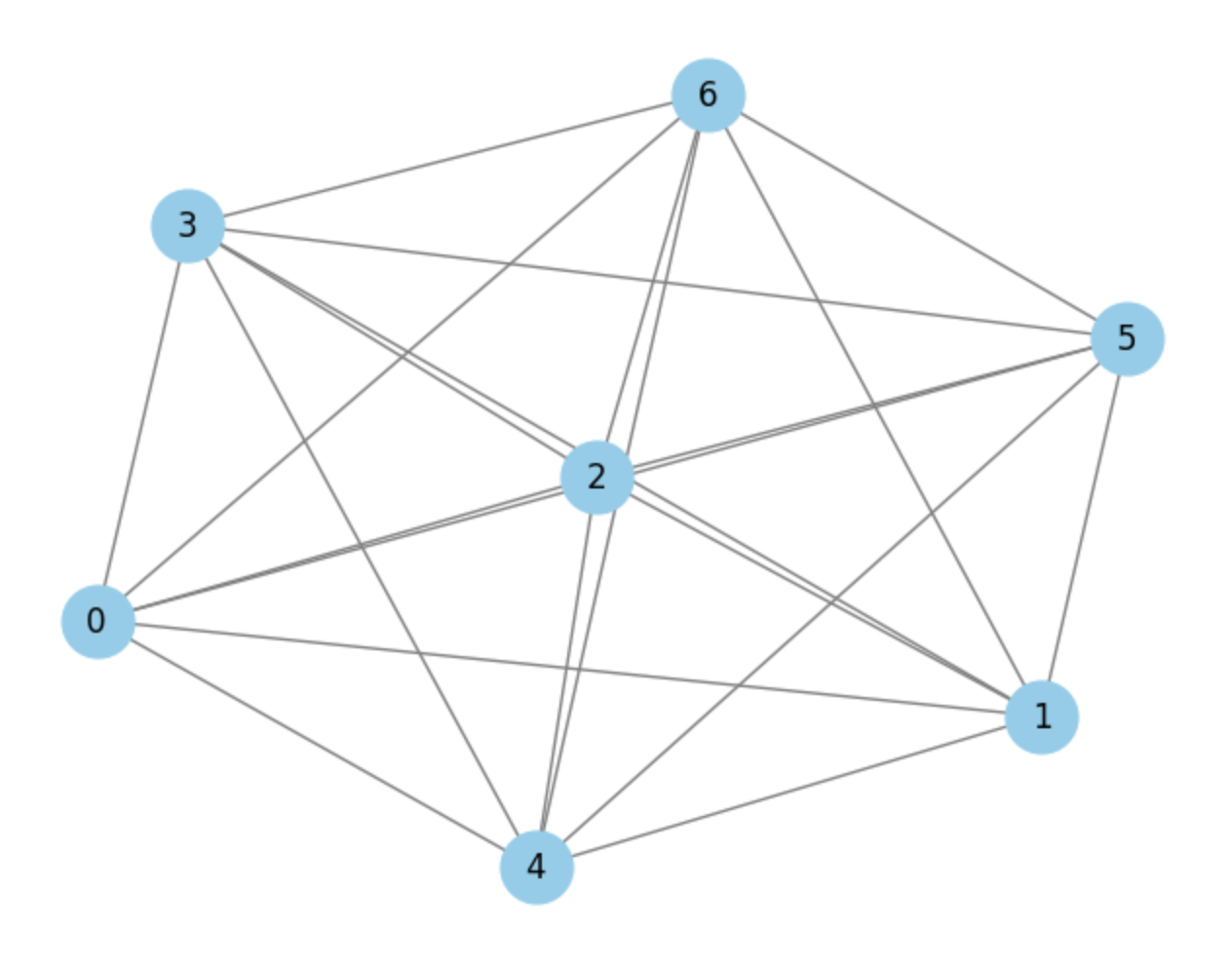
4.2 Each feature extracted as a Node of the Graph:

Each trigger station has extracted 7 features. Here each feature is considered to be a node of the graph and the values of these features extracted from 4 stations become the node features. A fully connected graph is created from these nodes like Figure 2.

Figure 1: Each station as a Node of the Graph

Figure 2: Each feature as a Node of the Graph

5 Model and Training

Message passing in GNNs enables nodes to exchange information with their neighbors. Nodes aggregate messages from adjacent nodes and update their own features based on these aggregated messages. This process helps nodes learn from their local graph structure and refine their representations iteratively. Once the representations are refined we can perform any downstream task like classification.

5.1 Message Passing in Our Model

In our model, the message-passing mechanism is designed as follows:

Message Computation:

• mlp1: A linear layer that computes the raw message from node $i$ to node $j$ by transforming the concatenated features $x_{i}$ and $x_{j}-x_{i}$:

  $$\text{msg}_{i\to j}=\text{ReLU}(\text{mlp1}(\text{concat}(x_{i},x_{j}-x_{i})))$$

  where ReLU (Rectified Linear Unit) introduces non-linearity Nair and Hinton (2010).

• mlp2: A linear layer applied to node features $x$ to transform them from the input dimension to the output dimension:

  $$x=\text{ReLU}(\text{mlp2}(x))$$

Weight Calculation:

• mlp3 and mlp4: Linear layers that compute scalar weights $w_{1}$ and $w_{2}$ based on the concatenated node features and messages. These weights are computed using the Sigmoid activation function Rumelhart et al. (1986):

  $$w_{1}=\text{Sigmoid}(\text{mlp3}(\text{concat}(x,\text{msg})))$$

  $$w_{2}=\text{Sigmoid}(\text{mlp4}(\text{concat}(x,\text{msg})))$$

• mlp5 and mlp6: Linear layers that project node features and messages into a lower-dimensional space (16 dimensions) for attention weight computation. These weights are derived using the Tanh activation function De Ryck et al. (2021):

  $$w_{1}=\text{Tanh}(\text{mlp5}(x_{i}))$$

  $$w_{2}=\text{Tanh}(\text{mlp6}(\text{msg}_{i\to j}))$$

• mlp7: Computes the final attention weight $w$ from the product of $w_{1}$ and $w_{2}$, normalized using the Softmax function Bridle (1989):

  $$w=\text{Softmax}(\text{mlp7}(w_{1}\cdot w_{2}),\text{edge\_index}[0])$$

Aggregation and Update:

• The final node feature $x^{\prime}$ is computed as a weighted sum of the messages and the node’s own features:

  $$x^{\prime}=w_{1}\cdot\text{msg}_{i\to j}+w_{2}\cdot x_{i}$$

  where $w_{1}$ and $w_{2}$ adjust the contributions from the message and node features, respectively.

5.2 Loss Function

To effectively train our model, we introduce a custom loss function that combines the mean squared error (MSE) with domain-specific penalties for predictions outside a lower limit $L$.

The loss function is defined as:

$$\mathcal{L}=\frac{1}{n}\sum_{i=1}^{n}\left[(y_{i}-\hat{y}_{i})^{2}+\mathbf{1}_{\{\hat{y}_{i}>L\}}\left(\frac{1}{1+e^{-3(\hat{y}_{i}-L)}}-1\right)-\mathbf{1}_{\{\hat{y}_{i}\leq L\}}\cdot\frac{1}{2}\right]$$ (1)

where:

• $(y_{i}-\hat{y}_{i})^{2}$: This is the Mean Squared Error between the true $y_{i}$ and the predicted value $\hat{y}_{i}$.

• $\mathbf{1}_{\{\hat{y}_{i}>L\}}$: An indicator function that applies a logistic penalty when the prediction $\hat{y}_{i}$ exceeds the lower limit $L$, ensuring smoother penalties as predictions exceed this threshold.

• $\mathbf{1}_{\{\hat{y}_{i}\leq L\}}$: An indicator function that applies a fixed penalty of $-\frac{1}{2}$ when $\hat{y}_{i}$ is less than or equal to $L$, discouraging predictions below this limit.

• $L$: The lower threshold limit, representing a critical boundary below which predictions are penalized more harshly.

5.3 Training

The GNN models were trained for 50 epochs on a single P100 GPU, taking approximately 2.5 hours when 7 nodes were taken and 45 minutes when 4 nodes where taken. The training utilized the Adam optimizer with a learning rate of 0.0002 and a weight decay of 5e-4.‘ReduceLROnPlateau‘ scheduler was employed to adjust the learning rate during training.

6 Results and discussion

We come up with 2 observations seeing Table 1. First that the Graph with higher node features is able to capture the information of the particle more accurately compared to the one with smaller node feature. Second is that the GNN based model gives lesser Mean Average Error(MAE) compared to the TabNet models.

Model	MAE	Params	Inf. Speed	Epochs to
				Converge
TabNet	0.8855	7,488	0.0193 ms	20
GNN (4-dim node feat.)	0.8850	99,952	0.1391 ms	47
GNN (7-dim node feat.)	0.8474	101,152	0.114 ms	18

Table 1: Comparison of models on MAE, parameter count, inference speed, and convergence.

Model	MAE	MSE	Avg Inference Time (micro-sec)	No. of Parameters
TabNet	0.9607	2.9746	458.7	6696
GNN-bendAngle	1.202931	3.520059	522.204	5579
GNN-bendAngle2	1.215189	3.605358	530.19	5903
GNN-etaValue	1.146910	3.240220	522.204	5579
GNN-etaValue2	0.992087	2.525927	530.19	5903
GNN-etaValue3	1.145697	3.276628	614.565	6437
GNN-etaValue4	1.133285	3.205457	267.509	6112
GNN-etaValue5	0.941620	2.312492	515.472	6545
GNN-etaValue6	0.946957	2.286622	283.216	14176

Table 2: Comparison of TabNet and GNN Models

7 Conclusion

In summary, our study demonstrates the effectiveness of Graph Neural Networks (GNNs) in analyzing data from CMS trigger stations. The GNN model, which captures both local and global graph structures, outperformed traditional methods like TabNet, indicating its potential for more accurate and insightful analysis in high-energy physics experiments.

8 Acknowledgement

9 Broader Impact

The use of GNN models for estimating momentum in CMS can give us a better efficiency of the trigger systems. It opens us a new domain to explore and achieve higher efficiency of the triggers and also understand high energy physics in a better way.