The Collective Voice of Ly$\alpha$ Emitters: Insights from JWST Stacked Spectroscopy

How Ly$\alpha$ photons escape from galaxies during the first billion years remains a central question for understanding early galaxy evolution and cosmic reionization. While Ly$\alpha$ emitters (LAEs) are known to be metal-poor and highly ionized, most studies rely on spatially integrated measurements, leaving the internal connection between Ly$\alpha$ emission, chemical enrichment, and feedback largely unexplored. We present a spatially resolved stacked analysis of 287 LAEs at $z>4$ observed with JWST/NIRSpec prism spectroscopy. By constructing a two-dimensional stack from public surveys (CAPERS, CEERS, JADES, and RUBIES), we probe the average internal structure of typical LAEs ($z_{\rm median}=5.5$, $M_{\rm UV,median}=-18.7$, EW(Ly$\alpha$)_median = 61 Å) on sub-kiloparsec scales. We find a clear radial decoupling between resonant and non-resonant emission: while EW(Hβ) and other optical lines decline with radius, EW(Ly$\alpha$) increases toward the outskirts, and the Ly$\alpha$ escape fraction rises from $\sim 16\%$ in the center to $\gtrsim 24\%$ at larger radii. This behavior indicates that resonant scattering redistributes Ly$\alpha$ photons into lower-density outer regions, where escape becomes more efficient. Optical diagnostics and $T_{e}$ measurements reveal low metallicities ($12+\log(\rm O/H)\simeq 7.7\pm 0.2$), high ionization parameters, negligible dust attenuation, and systematically elevated N/O ratios ($\log({\rm N/O})\sim-0.4$). The latter place typical LAEs among the growing population of nitrogen-enhanced high-redshift galaxies, pointing to rapid and possibly feedback-driven chemical enrichment. The inferred ionizing photon production efficiency, $\log(\xi_{\rm ion}/{\rm Hz\,erg^{-1}})\simeq 25.2$, together with the high Ly$\alpha$ escape fractions, suggests that these systems are efficient, though not extreme, contributors to the ionizing photon budget. Comparison with SPICE radiation-hydrodynamic simulations shows that bursty supernova feedback models naturally reproduce the observed radial trends in Ly$\alpha$ escape, UV slope, and emission-line equivalent widths, linking the spatial redistribution of Ly$\alpha$ to stochastic star formation and feedback-driven gas flows. Our results demonstrate that Ly$\alpha$ emission, chemical enrichment, and feedback are tightly connected in typical $z>4$ LAEs, and highlight the power of spatially resolved stacking with JWST to uncover the internal physical drivers of early galaxy evolution.

1 Introduction

Figure 1: From top to bottom: EW(Ly$\alpha$), $M_{\rm UV}$ vs redshift in our sample of 287 LAEs. Histograms reporting the distributions of rest-frame EW(Ly$\alpha$), $M_{\rm UV}$, and redshift are also shown at the side of the main panels.

Figure 2: 2D stacked spectrum of 287 LAEs using the NIRSpec/MSA prism spectra of LAEs at $z>4$. One pixel corresponds to 0.1 arcsec on the y-axis. Some of the brightest detected emission lines are marked with a vertical dashed white line.

Figure 3: Spectrum extracted from pixel 0 of the LAEs stack. (Top) Best-fit models to the observed data (blue solid line) are shown as solid coloured lines. Different colors mark different wavelength groups for which the fit is performed independently, as described in Sect. 3. (Bottom) Residuals of the best-fitting models shown in the top panel. 1$\sigma$ noise level is reported as shaded blue region.

Ly$\alpha$ emitters (LAEs) represent a fundamental population of galaxies in the early Universe. Characterized by strong Ly$\alpha$ emission and typically faint UV continua, LAEs are thought to trace low-mass, metal-poor systems with intense star formation (e.g., Kornei et al., 2010; Verhamme et al., 2018; Ono et al., 2010). Because Ly$\alpha$ photons are resonantly scattered by neutral hydrogen, their escape depends sensitively on the geometry, kinematics of the gas, as well as on the geometry of the dust (Verhamme et al., 2006). As a result, LAEs provide a unique laboratory for studying the interplay between star formation, interstellar medium (ISM) properties, and radiative transfer at high redshift (e.g., Kusakabe et al., 2022; Jung et al., 2024).

Over the past decade, large photometric and spectroscopic surveys have established LAEs as a key feature found in the galaxy demographic at $z>4$, spanning the epoch of reionization and its immediate aftermath. Their low metallicities, blue UV slopes, and high ionization parameters suggest that LAEs may represent an early evolutionary phase of star-forming events, potentially linked to efficient production of ionizing photons (Wilkins et al., 2011; Cullen et al., 2023; Napolitano et al., 2023). The presence of strong Ly$\alpha$ emission is in general an indication of non negligible escape of Lyman continuum photons (e.g., Marchi et al., 2018; Pahl et al., 2024) and, for this reason, LAEs are also thought to be key contributor to cosmic reionization (e.g., Saxena et al., 2024; Matthee et al., 2022). However, most observational constraints on LAEs have relied on spatially integrated measurements, limiting our ability to connect Ly$\alpha$ emission to the internal physical conditions of galaxies.

Understanding the spatial origin of Ly$\alpha$ emission is particularly critical. Observations have shown that Ly$\alpha$ halos can be significantly more extended than the UV continuum, indicating that resonant scattering redistributes Ly$\alpha$ photons over large spatial scales and that Ly$\alpha$ photons may also be scattered by the circum-galactic medium (Leclercq et al., 2017; Kusakabe et al., 2022; Hayes et al., 2014; Steidel et al., 2011). At higher redshifts, direct spatially resolved studies are far more challenging due to the intrinsic faintness and compactness of LAEs. As a consequence, it has been unclear how Ly$\alpha$ emission relates to the distribution of stars, metals, and ionized gas within early galaxies, and whether spatial gradients in metallicity, ionization, or dust play a dominant role in regulating Ly$\alpha$ escape.

The advent of the James Webb Space Telescope (JWST, Gardner et al., 2006, 2023) has transformed this landscape. In particular, NIRSpec prism observations provide continuous spectral coverage from the rest-frame UV to the optical at $z>4$, enabling simultaneous access to Ly$\alpha$, UV metal lines, Balmer recombination lines, and key optical diagnostics such as [O ii]λλ3726,3729, [O iii]λ5007, and [N ii]λλ6548,6584. Although the prism mode operates at low spectral resolution ($R\simeq 30$–300), its unprecedented sensitivity allows the detection of faint emission lines in galaxies that were previously accessible only through narrow-band Ly$\alpha$ surveys (e.g., Jones et al., 2024; Kageura et al., 2025; Tang et al., 2024; Yamada et al., 2012; Inoue et al., 2020; Umeda et al., 2025).

Early JWST observations have already revealed the remarkable diversity of physical conditions in high-redshift galaxies, including extreme ionization states, low metallicities, and signatures of chemical enrichment that challenge simple evolutionary models. At the same time, JWST has enabled the first systematic detection of rest-frame optical lines in large samples of LAEs, opening a new window onto their ionized gas properties. However, even with JWST, spatially resolved spectroscopy of individual LAEs remains feasible only through deep observations, with the most notable case being GN-z11 $z=10.6$ which shows a 0.4^′′ Ly$\alpha$-UV peak offset and a $\sim$0.78^′′ extended Ly$\alpha$ profile (Maiolino et al., 2024b; Scholtz et al., 2024).

Stacking techniques therefore provide a powerful complementary approach to extract key spectral features and infer physical properties across objects of similar nature. By co-adding spectra from large samples of galaxies, stacking enables measurements of average properties that would otherwise be inaccessible. When applied to two-dimensional spectra, 2D spectral stacking can preserve spatial information, allowing radial trends to be studied statistically even when individual objects are too faint to be well detected (Tripodi et al., 2024).

In this work, we exploit the growing archive of JWST/NIRSpec prism observations to perform a spatially resolved stacked analysis of LAEs at $z>4$. We compile a sample of 287 LAEs drawn from multiple public surveys across the COSMOS, EGS, UDS, and GOODS-N/S fields, making this one of the largest spectroscopic samples of high-redshift LAEs assembled to date. By stacking, we achieve high signal-to-noise ratios while retaining radial information on scales of $\sim 0.1^{\prime\prime}$, corresponding to sub-kiloparsec physical distances at the median redshift of the sample.

This stacking strategy allows us to investigate, in a uniform and self-consistent framework, how Ly$\alpha$ emission relates to UV continuum slopes, Balmer recombination lines, metal-line diagnostics, and chemical abundances as a function of radius. In particular, we use a combination of empirical diagnostics, photoionization models, and direct electron-temperature measurements to constrain metallicity, ionization parameter, and nitrogen enrichment. We further estimate Ly$\alpha$ escape fractions and the ionizing photon production efficiency, $\xi_{\rm ion}$, and explore how these quantities vary spatially within the stacked galaxies.

By combining the statistical power of stacking with the broad wavelength coverage of JWST, this work provides a population-level view of the internal structure of LAEs during the first billion years of cosmic history. Our results offer new insights into the physical mechanisms governing Ly$\alpha$ escape, chemical enrichment, and ionizing photon production in early galaxies, and demonstrate the effectiveness of stacked JWST spectroscopy as a tool for studying systems beyond the reach of individual observations.

Throughout the paper we adopt AB magnitudes (Oke & Gunn, 1983) and the $\Lambda$CDM cosmology from Planck Collaboration et al. (2020): $H_{0}=67.4\penalty 10000\ \rm km\penalty 10000\ s^{-1}\penalty 10000\ Mpc^{-1}$, $\Omega_{m}=0.315$, and $\Omega_{\Lambda}=0.685$.

2 A sample of Ly$\alpha$ emitters at $z>4$

The aim of this study is to investigate the connection between Ly$\alpha$ emission and rest-frame UV and optical properties of Ly$\alpha$ emitters (LAEs) at $z>4$ using spatially resolved spectroscopy. For this purpose, JWST/NIRSpec Multi Shutter Array (MSA) prism observations offer the optimal combination of broad spectral coverage ($\sim$0.6–5.3 $\mu$m) and high sensitivity, despite their relatively low spectral resolution ($R\simeq 30$–300). We compiled all publicly available NIRSpec/prism spectroscopy from the DAWN JWST Archive(DJA, Heintz et al., 2024; de Graaff et al., 2025), covering the COSMOS (Scoville et al., 2007), EGS (Davis et al., 2007), UDS (Lawrence et al., 2007), and GOODS-N/S fields (Grogin et al., 2011; Koekemoer et al., 2011).

In particular, for the GOODS-N/S fields we considered the catalog of 82 LAEs identified by Jones et al. (2025). Similarly, for the EGS and UDS fields we adopted the LAEs samples reported by Napolitano et al. (2024) and Napolitano et al. (2025b), comprising 42 and 74 LAEs, respectively. We then complemented these samples with new LAE identifications from the CANDELS-Area Prism Epoch of Reionization Survey (CAPERS; GO-6368, PI Mark Dickinson). CAPERS observed a total of 21 NIRSpec pointings, uniformly distributed across the COSMOS, UDS, and EGS fields, using the prism configuration. For CAPERS targets, we used the internal CAPERS data reduction which follows the general procedures outlined in Arrabal Haro et al. (2023). Details of the survey strategy, target selection, data reduction, and redshift identification are provided in the collaboration papers (e.g., Napolitano et al., 2025b; Taylor et al., 2025).

Background subtraction was performed using local background estimates from adjacent shutters. As a result, some degree of self-subtraction may affect the 2D spectra of the most spatially extended sources at distances beyond $\pm 2.5$ off-centered pixels. In our analysis, however, we restrict the measurements to pixels within $\pm 2$, and therefore our results are not expected to be significantly biased by potential self-subtraction effects.

Whenever available, we also considered spectroscopic redshifts and the absolute UV magnitude (M_UV) provided by literature. For unpublished sources, we derived the redshift and M_UV from the line centroids of rest-frame optical emission lines and the median observed flux averaged over 1450–1550 Å, respectively (see Napolitano et al., 2025b, for details).

We note that for the identification of additional LAEs in CAPERS, we applied the same methodology adopted in the aforementioned studies (Napolitano et al., 2024; Jones et al., 2025; Napolitano et al., 2025b). Briefly, due to the low spectral resolution of the 1D NIRSpec prism data, Ly$\alpha$ emission is modeled within a $\sim$ 4–5 pixels window centered on the observed emission peak at the expected Ly$\alpha$ wavelength. As a first step, the line flux is computed via direct integration over this window. The continuum is estimated through a linear fit to the red side of Ly$\alpha$, spanning from 1900 Å to three pixels red-ward of the emission peak. To further refine the measurement, we adopt a forward-modeling approach. We construct a library of Gaussian emission profiles with full widths at half maximum (FWHM) uniformly sampled in the range 100–1500 km s^-1. We note that star-forming galaxies at z $\sim$ 5–7 were found to have Ly$\alpha$ FWHM $\sim$ 300 km s^-1 (e.g., Pentericci et al., 2018; Tang et al., 2024). The assumed range of FWHM have been adopted to sample properties of star-forming LAE with a broad prior. For each profile, the amplitude is drawn from a uniform distribution constrained to produce an integrated flux within a factor of 0.2–5 of that obtained from direct integration. Each Gaussian profile is combined with a step-function continuum: the red side is given by the linear fit, while the blue side is fixed to the median flux blue-ward of the line, accounting for intergalactic medium absorption. The full model is convolved with a Gaussian kernel ($\sigma_{R}(\lambda_{\mathrm{obs}})$), matching the instrumental resolution. The fit is performed using a Markov Chain Monte Carlo (MCMC) analysis implemented with the emcee package (Foreman-Mackey et al., 2013), using 10 walkers and 20,000 steps. The best-fit Ly$\alpha$ flux and rest-frame equivalent width (EW₀, hereafter just EW) are derived from the posterior medians, with uncertainties given by the 68th percentile intervals. Overall, following this procedure, we identified 83 and 87 additional LAEs in the CAPERS-EGS and CAPERS-COSMOS fields, respectively.

By selecting sources with signal-to-noise ratio (S/N) on the EW of Ly$\alpha$ $>3$, we considered a total of 368 LAEs at z $>$ 4 across the COSMOS, EGS, UDS, and GOODS-N/S fields. All spectra were visually inspected to ensure data quality, and the following additional selection criteria were applied to guarantee the robustness of the analysis. First, to minimize AGN contamination, we excluded known broad-line AGNs reported in the literature (e.g., Maiolino et al., 2024a; Juodžbalis et al., 2026), as well as objects identified through visual inspection, removing 24 sources ($\sim 6\%$ of the initial sample). Second, we discarded spectra affected by strong artifacts, including multiple spurious spikes in the spectral region of interest or severe truncation due to the physical gap between the NIRSpec detectors. Third, we excluded LAEs whose spectra were contaminated by nearby secondary sources. The final sample comprises 287 LAEs at $z>4$.

Fig. 1 presents the distribution of the final sample in rest-frame equivalent width of Ly$\alpha$ (EW(Ly$\alpha$)), $M_{\mathrm{UV}}$, and redshift. The sample has a median EW_median(Ly$\alpha$)$=61$ Å and a median $M_{\mathrm{UV,median}}=-18.7$, with 16th and 84th percentiles at $M_{\mathrm{UV}}=-17.9$ and $-19.7$, respectively. The median redshift of the sample is $z_{\rm median}=5.5$, with 16th and 84th percentiles at $z=4.6$ and $=6.8$, respectively. This corresponds to a median angular scale of $6.113\penalty 10000\ \rm kpc/"$, which we adopt as the reference distance to angular conversion scale, hereafter.

Figure 4: [N ii]λ6584/Hα vs [Ne iii] _blend/[O ii]. Our observed ratios in pixels $0$, $\pm 1$ are compared with models from the NUVOLOSO project (Pérez-Díaz et al. in prep.) at $\log(n)[\rm cm^{-3}]=2.0$ (gray scale) and $\log(n)[\rm cm^{-3}]=3.0$ (coloured scale). The grid is color-coded by discrete values of ionization parameter, $\log(U)$, and nitrogen abundance, $\log(\rm N/O)$, as reported in the respective color bars.

3 Methods

Table 1: EW₀ of the fitted emission lines.

Line	Pix -2	Pix -1	Pix 0	Pix 1	Pix 2
Ly$\alpha$	$63\pm 5$	$33\pm 1$	$30\pm 1$	$35\pm 1$	$74\pm 6$
C II†	–	–	–	$1.3\pm 0.7$	–
Si IV†	–	–	–	$2\pm 1$	–
C IV	–	–	$7\pm 1$	$7\pm 2$	–
O iii]λ1666 +He ii	–	$8\pm 1$	$10\pm 2$	$21\pm 3$	–
C III]	$18\pm 5$	$17\pm 3$	$9\pm 1$	$20\pm 2$	$16\pm 4$
He i λ3487	–	–	–	$9\pm 2$	–
[O ii]λλ3726,3729	$45\pm 8$	$49\pm 2$	$38\pm 1$	$49\pm 2$	$80\pm 8$
[Ne iii]λ3869 +Hζ +Hη +He i λ3889	$57\pm 7$	$60\pm 3$	$60\pm 1$	$57\pm 3$	$68\pm 8$
Hδ	$27\pm 6$	$24\pm 2$	$26\pm 1$	$19\pm 2$	$26\pm 5$
Hγ + [O iii]λ4363	$76\pm 12$	$65\pm 7$	$83\pm 2$	$71\pm 6$	$95\pm 15$
He i λ4471	–	$6\pm 2$	$9\pm 1$	$4\pm 2$	–
He II	–	$4\pm 2$	$12\pm 2$	$8\pm 2$	–
Hβ	$144\pm 10$	$160\pm 5$	$175\pm 3$	$155\pm 4$	$162\pm 10$
[O iii]λ5007	$716\pm 23$	$847\pm 14$	$938\pm 12$	$846\pm 13$	$709\pm 26$
He i λ5876	$71\pm 15$	$47\pm 5$	$41\pm 3$	$31\pm 3$	–
Hα	$<722$	$775_{-74}^{+34}$	$837\pm 30$	$769\pm 46$	$<892$
[N II]	–	$76_{-21}^{+55}$	$83\pm 20$	$129\pm 33$	–
[S ii]	–	$22\pm 6$	$30\pm 5$	$27\pm 6$	–
He i λ7065	–	$15\pm 5$	$20\pm 3$	$17\pm 4$	–
[Ar iii] †	–	–	$7\pm 3$	$9\pm 3$	–††
[O ii] λλ7319,7330	–	–	$16\pm 5$	–	–

Notes. Columns: line name, EW₀ in different pixels from -2 to 2 in units of Å. The symbol ^† marks tentative detections. ^††: we find a tentative detection of [Ar iii] in pix 2, but the continuum level is too noisy to derive a reliable estimate of its EW.

3.1 Stacking procedure

To maximize the S/N across the spectrum, we performed a stacked analysis of the parent sample of 287 LAEs (see Sect. 2). Specifically, we constructed a composite two-dimensional (2D) spectrum of LAEs at $z>4$ by stacking their JWST/NIRSpec prism observations. Prior to stacking, each individual spectrum was de-redshifted, interpolated onto a common rest-frame wavelength grid, and normalized by the rest-frame UV continuum flux at $\lambda_{\rm rest}=1500\penalty 10000\ \text{\AA }$ derived from $M_{\rm UV}$ (see Sect. 2). All spectra were spatially aligned with respect to the galaxy center, defined as the brightest pixel in continuum and emission-line flux. Specifically, we first computed the sum of the flux over the whole spectral wavelength range for each spatial pixel; then, we fitted this spatial flux profile with a Gaussian, and we adopted the value of the peak pixel as the galaxy center. This is a commonly established method for deriving the center of a source in 2D spectra (see e.g. appendix A in Castellano et al., 2025), and the results have been verified by visual inspection. This alignment is essential for obtaining reliable radial profiles of both line and continuum emission.

The composite flux in each wavelength and spatial bin was computed as the median of the flux distribution across the stacked spectra. We chose to adopt the median stacking over the average stacking for two main reasons: (1) to allow a fair comparison with results from other studies in the literature (e.g., Roberts-Borsani et al., 2024; Isobe et al., 2025); (2) the median approach is known to mitigate the contribution of outliers, producing spectra that better represent the average properties of individual galaxies. Associated uncertainties were estimated as the semi-difference between the 16th and 84th percentiles of the flux distribution in each bin, divided by the square root of the number of stacked galaxies. We verified that this approach yields the most conservative uncertainty estimates when compared to standard error propagation or to the dispersion measured from 1000 stacked spectra generated by randomly perturbing individual spectra within their errors (see also Roberts-Borsani et al., 2024; Isobe et al., 2025). Therefore, percentile-based uncertainties simultaneously capture the statistical error of the individual spectra and the intrinsic variation in physical properties across the galaxy population, which we intentionally preserve when modelling the stacked spectrum and inferring physical parameters.

The final 2D stacked spectrum is shown in Fig. 2. The five central spatial pixels ($0,\penalty 10000\ \pm 1,\penalty 10000\ \pm 2$) exhibit significant continuum and emission-line signal, while in pixels $\pm 3$ only a tentative Ly$\alpha$ detection is observed (see Sect. 5.4 for discussion). We note that the angular distance between adjacent spatial pixels is 0.1$"$ (Jakobsen et al., 2022; Böker et al., 2023).

3.2 Spectral modelling

From the stacked 2D spectrum, we extracted one-dimensional (1D) spectra for each spatial pixel in the range $[-3,3]$ (see Fig. 2) and fitted them independently. Emission lines and continuum were modelled using a Bayesian framework based on MCMC sampling, implemented with the emcee package (Foreman-Mackey et al., 2013). Given the large wavelength coverage of each spectrum, the fitting was performed over separate wavelength intervals, simultaneously modelling emission lines and continuum within each interval (see, e.g., the coloured fits in Fig. 3). The continuum was described by a power-law model ($F_{\lambda}\propto\lambda^{\alpha}$), with free slope and normalization. All emission lines, except Ly$\alpha$ and blended lines, were modelled with a single Gaussian profile, with free peak flux, central wavelength, and velocity dispersion, yielding posterior distributions for all parameters. To model blends of unrelated species (i.e., O iii]λ1666 +He II, Hγ +[O iii]λ4363), we adopted two Gaussians, as this provides a better representation of the observed profile than a single Gaussian; however, due to the strong degeneracy of the fit, we do not attempt to decompose the individual components and instead consider only the total blended flux. For emission-line doublets with fixed wavelength separation and intrinsic flux ratios, the number of free parameters was reduced by fixing the relative peak fluxes and wavelength offsets to their atomic values and enforcing a common line width (e.g., [Ne iii]λλ3869,3967, [N ii]λλ6548,6584, [O iii]λλ4959,5007; see Tripodi et al. 2024 for details).

Line fluxes, widths, and rest-frame equivalent widths were derived from the median (50th percentile) of the posterior distributions, with uncertainties estimated as the semi-difference between the 16th and 84th percentiles. The EW of all detected and tentative emission lines are reported in Tab. 1. Line ratios used in Sect. 4 and in the discussion of Sect. 5 are reported in Tab. 3.

Thanks to the high S/N achieved in the central spatial pixels ($0,\penalty 10000\ \pm 1$), we were able to robustly constrain the contribution of [N ii]λλ6548,6584 (hereafter [N II]) to the Hα emission. Specifically, the inclusion of the [N II] component is strongly favored, with a difference in the Bayesian Information Criterion of $\Delta(\mathrm{BIC})>10$ when comparing fits with and without [N II] (see Fig. 12 in Appendix B). This level of constraint is not achieved in the $\pm 2$ pixels; therefore, all measurements reported for Hα in these outer pixels correspond to the blended Hα +[N II] emission.

Given the asymmetric shape of the underlying continuum adjacent to the Ly$\alpha$ emission line, caused by the presence of the Ly$\alpha$-break blueward of the emission, we fitted the continuum in the rest-frame 1250–1500 Å wavelength range using a linear model implemented with the scipy curve_fit package. The Ly$\alpha$ emission line in the stacked galaxy spectra is intrinsically asymmetric, reflecting the dispersion in velocity offset compared to the systemic redshift of the LAEs sample, commonly observed in individual LAEs (e.g., Verhamme et al., 2018; Jung et al., 2024; Prieto-Lyon et al., 2025). As a result, a single Gaussian profile does not adequately represent the observed emission of the stack. Therefore, we measured the Ly$\alpha$ line flux via direct integration over the rest-frame 1200–1240 Å wavelength window. The EW(Ly$\alpha$) was then derived from the measured Ly$\alpha$ flux and the continuum level extrapolated at the wavelength corresponding to the Ly$\alpha$ peak.

4 Data Analysis and Results

Figs. 3, 10 and 11 present the observed stacked spectra for each spatial element in the 2D spectrum along with the best-fit models. Emission lines are detected in 5 different spatial pixels, namely pixels 0, +1, -1, +2, -2 in increasing order of distance from the center (i.e., pixel 0). In the following sections, we report the main findings concerning the spatially resolved spectral properties in our stack of LAEs.

Differently from non-LAEs (see e.g., Roberts-Borsani et al., 2024), LAEs exhibit a rich set of bright emission lines spanning both the rest-frame UV and optical wavelength ranges. In the UV, Ly$\alpha$ emission is detected from the central regions out to the outskirts. Among the metal and helium lines, C iii] is robustly detected at all radii, while O iii]λ1666 +He ii λ1640 and He ii λ4686 are detected only in the central spatial pixels ($0,\pm 1$). Notably, also C iv emission is observed exclusively in the central pixels, suggesting that the physical conditions required to produce high-ionization lines are confined to the innermost regions.

In the optical regime, [O ii]λλ3726,3729 (hereafter [O ii]λ3727), [Ne iii], the Balmer series down to Hδ, [O iii]λ5007, and He i λ5875 are detected from the center to the outer spatial pixels. Additional optical lines, including He i λ4471, [S ii], and He i λ7065, are detected only in the central regions ($0,\pm 1$), and [O II]λλ7319,7330 (hereafter [O ii]λ7320) just in the central pixel. Tentative detections of Ar III are also found in pixels $0$ and $+1$. Other tentative detections are listed in Tab. 1.

We report the results for the EWs of all emission lines in Tab. 1, and we will discuss the implications for the properties of LAEs in Sect. 5.4.

Table 2: UV slopes, metallicity and nitrogen-over-oxygen abundance

	$\beta_{\rm UV}$	$\log(Z_{\rm Sanders}/Z_{\odot})$	$\log(Z_{\rm direct}/Z_{\odot})$	$\log(Z_{\rm\textsc{HCm}}/Z_{\odot})$	$\log(\rm N/O)_{\rm\textsc{HCm}}$
Pix 2	$-2.5\pm 0.1$	$-1.38\pm 0.05$	$-1.20\pm 0.03$	$-0.96\pm 0.02$	N/A
Pix 1	$-2.07\pm 0.02$	$-1.20\pm 0.03$	$-0.85\pm 0.02$	$-0.85\pm 0.04$	$-0.3\pm 0.2$
Pix 0	$-1.95\pm 0.02$	$-1.22\pm 0.02$	$-0.93\pm 0.01$	$-0.91\pm 0.02$	$-0.5\pm 0.4$
Pix -1	$-2.32\pm 0.01$	$-1.23\pm 0.03$	$-0.80\pm 0.02$	$-0.90\pm 0.07$	$-0.8\pm 0.4$
Pix -2	$-2.29\pm 0.05$	$-1.26\pm 0.05$	$-1.04\pm 0.04$	$-1.00\pm 0.05$	N/A

Notes. Columns: UV continuum $\beta$ slope; metallicity computed from the calibrations reported in Sanders et al. (2025); metallicity computed from the $T_{e}$-direct method using models from NUVOLOSO project (see Sect. 5.2); metallicity computed from HCm; N/O abundance computed from HCm.

4.1 Photoionization models

In this section, we briefly describe the photoionization models retrieved from the ‘detailed analysis of Nebular UltraViolet and Optical emission Lines to Optimize Studies of the iOnized gas’ (NUVOLOSO) project (Pérez-Díaz et al. in prep), which will be used in the analysis to derive key physical quantities such as gas-phase metallicity, ionization parameter and nitrogen-to-oxygen abundances.

Photoionization models were computed using Cloudy v25 (Gunasekera et al., 2025), where the ionizing source is SSPs accounting for binaries from BPASS v2.3 (Byrne et al., 2022) characterized by the same metallicity of the gas-phase ISM and accounting for a young burst with age of 1 Myr. Longer ages (up to 3 Myr) induces small differences in the chemical abundance derivation (e.g., Pérez-Montero, 2014).

Model grids have been derived covering a great range of the parameter space. In terms of chemical composition of the gas-phase, the explored metallicities range from 0.086 Z_⊙ (extremely metal-poor) to 1.8 Z_⊙ (super-solar) in steps of 0.2 dex. All elements are scaled following the solar proportions (Asplund et al., 2021), with the exception of N for which we explore alternative ratios from -2.0 to 0.5 and C which is scaled following log(C/N) = 0.6 (Berg et al., 2016; Steidel et al., 2016; Pérez-Montero & Amorín, 2017). By means of variations of log($U$) which is covered in the range of [-4.0, -1.0], we explore different scenarios accounting for the total number of ionizing photons released by the same SED shape, for fixed H density of 1000 cm^-3 and assuming the standard dust-to-gas ratio of the Milky Way. These models represent a small subset of the grid of models that constitute the NUVOLOSO project (Pérez-Díaz et al. in prep.).

4.2 Test of the observed [N ii]λ6584/Hα ratio

A robust determination of the [N ii]λ6584/Hα ratio is important for constraining the dust attenuation via Balmer decrements that include Hα. To further assess the reliability of the [N ii]λ6584/Hα ratios inferred from the best-fitting spectra in pixels $0$ and $\pm 1$ (see Sect. 3), we compared our measurements with predictions from the photoionization models of the NUVOLOSO project (see Sect. 4.1; Pérez-Díaz et al., in prep.).

We measure $\log(\text{[{N}\,{\sc{ii}}]{l}{6584}{}{}}/\text{Ha})=-1.0\pm 0.1$ in pixel $0$, $\log(\text{[{N}\,{\sc{ii}}]{l}{6584}{}{}}/\text{Ha})=-0.77\pm 0.15$ in pixel $+1$, and $\log(\text{[{N}\,{\sc{ii}}]{l}{6584}{}{}}/\text{Ha})=-1.0^{+0.2}_{-0.3}$ in pixel $-1$ (see also Tab. 3). As shown in Fig. 4, where [N ii]λ6584/Hα is compared with [Ne iii] _blend/[O ii], our measurements are in good agreement with model predictions at gas density $\log(n/\rm cm^{-3})=3$, supporting the robustness of the inferred [N ii]λ6584/Hα ratios despite the limited spectral resolution. Our results also match Hα/(Hα +[N ii]λλ6548,6584)$=0.96$ found in a stack of medium resolution grating spectra of $z>4$ galaxies (Sandles et al., 2024), and the [N ii]λ6584/Hα ratios found in a sample of 588 galaxies at $1.5<z<7$ using R$=1000$ grating spectra (see Fig. 3 in Cameron et al., 2026). As an additional consistency check, we derived the [N ii]λ6584/Hα ratio from the $R=1000$ grating spectra of a subset of our parent sample. In particular, for the 53 LAEs in JADES DR4 with available high-resolution spectroscopy (Curtis-Lake et al., 2025a, b), we measure an average value of $\log(\text{[{N}\,{\sc{ii}}]{l}{6584}{}{}}/\text{Ha})=-1.3\pm 0.5$. This result is consistent with the value inferred from our stacked spectrum within the uncertainties. The small offset between the two measurements may reflect differences in sample properties, as the JADES subsample is, on average, brighter in $M_{\rm UV}$ and characterized by lower EW(Ly$\alpha$) compared to the full stacked sample.

From the comparison with the models in Fig. 4, we also infer ionization parameters in the range $-2.0<\log({\rm U})<-1.5$ and nitrogen-to-oxygen abundance ratios spanning $-0.5<\log({\rm N/O})<0.0$. As an independent check, we also estimate the N/O abundance in pixel $0$, where the S/N is highest, using the empirical correlation between $\log({\rm N/O})$ and the [N ii]λ6584/[S ii] line ratio reported by Pérez-Montero & Contini (2009) and by Cataldi et al. (2025). This approach yields $\log({\rm N/O})=-0.3\pm 0.2$ and $=-0.5\pm 0.1$, respectively, which is consistent with the values inferred from the photoionization models within the uncertainties.

The implications of these constraints for the gas-phase metallicity and nitrogen enrichment are discussed in detail in Sects. 5.2 and 5.3, respectively.

4.3 UV slopes and dust correction

The blue UV continuum slopes, $\beta_{\rm UV}$, reported in Tab. 2 are derived from the best-fitting spectral models shown in Figs. 3, 10, 11, assuming $F_{\lambda}\propto\lambda^{\beta_{\rm UV}}$, and are measured within the interval 1300–2600 Å avoiding bright emission lines. This is approximately the standard Calzetti wavelength range (Calzetti et al., 1994), usually adopted to measure $\beta_{\rm UV}$.

A robust estimate of the dust attenuation, $A_{V}$, is required to reliably correct emission-line fluxes separated widely in wavelength. However, the low spectral resolution of NIRSpec/prism makes the determination of $A_{V}$ especially challenging in our data. In particular, the Balmer decrement Hα/Hβ is affected by blending between Hα and [N ii]λ6584; the Hβ/Hγ ratio critically depends on an accurate measurement of the [O iii]λ4363 line, which is blended with Hγ; while the Hβ/Hδ decrement is sensitive to the signal-to-noise ratio of the underlying continuum, which becomes progressively weaker and noisier in the outer spatial pixels. Indeed, the Hβ/Hδ ratio is only measured up to pixels $\pm 1$ with S/N$>4$.

Assuming that the [N ii]λ6584 contribution to Hα inferred from our best-fit models in pixels $0$ and $\pm 1$ is reliable (see Sect. 3 and Sect. 4.2), the resulting negative Hα/Hβ Balmer decrements are consistent with no dust attenuation at all radii. Balmer decrements below Case B are found even in high S/N individual spectra (e.g., Reddy et al., 2015), supporting no dust contribution. This scenario is in good agreement with the uniformly blue UV slopes observed across the spatial extent of the stacked LAEs.

From the Hβ/Hδ ratio, we infer instead higher dust attenuation values which increase radially ($A_{V}=0.7\pm 0.4,0.9\pm 0.5,2.1\pm 0.7$ in pixels $0,-1,1$), excluding the pixels $2,-2$ due to the low S/N. This trend, however, is at odds with the observed UV continuum slopes, which become progressively bluer toward the outskirts. Given the large uncertainties, the values are still consistent with Case B with no attenuation, within 2-3 $\sigma$. Therefore, in the following we adopt no dust attenuation in our analysis.

4.4 Line blending and contamination correction.

When measuring [Ne iii]λ3869, we explicitly account for flux contributions from Hη, Hζ ($\lambda=3890.17$ Å), and He i λ3889, all of which are blended with [Ne iii]λ3869 at the spectral resolution of the NIRSpec/prism. We define the total blended flux as $\text{[{Ne}\,{\sc{iii}}]{}{}{}{}}_{\rm blend}=\text{[{Ne}\,{\sc{iii}}]{l}{3869}{}{}}+\text{Hz}+\text{{He}\,{\sc{i}}{\,l}{3889}{}{}}+\text{Hh}$.

To estimate the contamination from these additional lines, we proceed as follows. For the Balmer lines Hζ and Hη, we measure the $\text{Hd}/\text{[{Ne}\,{\sc{iii}}]{}{}{}{}}_{\rm blend}$ flux ratio from the spectral fits, obtaining values in the range $0.3$–$0.4$. Assuming theoretical Balmer line ratios from Case B recombination with electron temperature $T_{\mathrm{e}}=10{,}000$ K and electron density $n_{\mathrm{e}}=10^{3}\penalty 10000\ \mathrm{cm}^{-3}$ (Storey & Hummer, 1995), this implies $\text{Hh}/\text{[{Ne}\,{\sc{iii}}]{}{}{}{}}_{\rm blend}=0.08$–$0.11$ and $\text{Hz}/\text{[{Ne}\,{\sc{iii}}]{}{}{}{}}_{\rm blend}=0.12$–$0.17$.

The contamination from He i λ3889 is estimated in the central pixels ($0$, $\pm 1$) using the detected He i λ5876 emission line, assuming Case B recombination (i.e., $\text{{He}\,{\sc{i}}{\,l}{5876}{}{}}/\text{{He}\,{\sc{i}}{\,l}{3889}{}{}}=1.19$). This yields $\text{{He}\,{\sc{i}}{\,l}{3889}{}{}}/\text{[{Ne}\,{\sc{iii}}]{}{}{}{}}_{\rm blend}=0.17$–$0.20$ (see Tab. 3). For the outer pixels ($\pm 2$), where no He I line is detected or the flux determination is compromised by the noisy continuum, we assume the same $\text{{He}\,{\sc{i}}{\,l}{3889}{}{}}/\text{[{Ne}\,{\sc{iii}}]{}{}{}{}}_{\rm blend}$ ratio as in the inner regions.

Combining all contributions, we obtain $(\text{Hz}+\text{Hh}+\text{{He}\,{\sc{i}}{\,l}{3889}{}{}})/\text{[{Ne}\,{\sc{iii}}]{}{}{}{}}_{\rm blend}=0.37$–$0.48$, which corresponds to $\text{[{Ne}\,{\sc{iii}}]{l}{3869}{}{}}/\text{[{Ne}\,{\sc{iii}}]{}{}{}{}}_{\rm blend}=0.52$–$0.63$ (see Tab. 3). Given the uncertainties associated with the assumption of no dust and the inferred He i λ3889 contribution, we present the line ratios involving [Ne iii]λ3869 corrected for blending in Fig. 13. The corrected values should be considered as lower limits on the intrinsic [Ne iii]λ3869 flux.

Figure 5: [O iii]λ5007/Hβ–[Ne iii]λ3869/[O ii]λ3727 line ratio (‘OHNO’) diagram for the LAE stack compared with observations and photo-ionization models. Spatially resolved ratios for our stack are plotted as solid circles in both panels and are colour coded based on the distance (in pixel) from the center of the galaxy (i.e., pixel 0). Error bars represent standard deviation. (Left) Our LAEs stack (coloured dots) is compared with $z\sim 0$ SDSS AGNs as blue colormap with contours, SMACS 06355, 10612 and 04590 red triangles; Trussler et al., 2023; the left-most square of the three is 06355, a type-II AGN identified by Brinchmann, 2023, high-z C III] emitters (orange squares, Arevalo-Gonzalez et al., 2025), a sample of galaxies at $z>2$ (yellow squares, Backhaus et al., 2024), a sample of star-forming galaxies in CEERS at $2.7<z<6.5$ (purple squares, Shapley et al., 2023), and at $7<z<9$ (green squares, Tang et al., 2023). Contours represent the percentiles (from 15% to 95% for SDSS with a step of 10%) of the number of objects in a sample. (Right) overlaid to our results (as in the left panel) are the photoionization models of Cameron et al. (2023); Katz et al. (2023) at hydrogen densities $\log n{\rm[cm^{-3}]}=2.0$ (gray scale grid) and $\log n{\rm[cm^{-3}]}=3.0$ (coloured scale grid). The grid shows the variation of the ionization parameter and metallicity (colour scales on the right-hand side of the figure, same limits are adopted for gray scale). To guide the eye, lighter colors represent lower metallicity and higher ionization. Y-axis is the same as the left panel.

5 Spatially resolved properties of Ly$\alpha$ emitters

5.1 UV slopes and Dust attenuation

Our stacked sample of $z>4$ LAEs exhibits progressively bluer UV continuum slopes $\beta_{\rm UV}$ with increasing radius, indicating a spatial variation in the underlying stellar populations and/or dust content. Our inferred UV slopes ($\beta_{\rm UV}\sim-2.2$ on average) are in good agreement with measurements for single LAEs at $z>5$ (Witstok et al., 2024, 2025), for a stack of 42 LAEs in JADES (Kumari et al., 2024), but also for star-forming galaxies at $z\sim 5$–7 and in the same $M_{\rm UV}$ range reported in the literature (Wilkins et al., 2011; Finkelstein et al., 2012; Bouwens et al., 2014; Nanayakkara et al., 2024; Cullen et al., 2023; Dottorini et al., 2025). When compared with the stacked LAEs presented in Roberts-Borsani et al. (2024), we find that the central UV slope in their stack is steeper than ours in the central pixel by a factor of $\sim 1.4$ (i.e., bluer), with $\beta_{\rm UV}=-2.59\pm 0.05$, while the agreement improves toward larger radii. However, we note that (i) Roberts-Borsani et al. (2024) measured $\beta_{\rm UV}$ in a much redder interval (1600-2800 Å) which intrinsically implies bluer slopes, also compared to other works (see detailed discussion in Dottorini et al., 2025); (ii) their UV slope is averaged over the spectral extraction window, which is 3-4 pixels; (iii) our parent sample includes approximately five times more LAEs than that of Roberts-Borsani et al. (2024), which may partially explain the differences observed in the central regions.

The observed radial trend in $\beta_{\rm UV}$ suggests a decreasing dust attenuation with radius, implying little to no dust contribution on the largest spatial scales probed by our stacks. This is consistent with our results from the Balmer decrement $\text{Ha}/\text{Hb}$. Indeed, blue UV slopes are found to be connected with the overall low dust content also in other single LAEs at similar redshifts (e.g., Kornei et al., 2010; Ono et al., 2010; Napolitano et al., 2023), as well as with the weak dust attenuation reported by Roberts-Borsani et al. (2024) in LAE stacks and by Witstok et al. (2024, 2025) in single LAEs. Alternatively, the trend may also reflect an increasing contribution from younger and/or more metal-poor stellar populations in the outskirts, highlighting the degeneracy between dust and stellar population effects when relying solely on UV continuum slopes. However, as discussed in Sect. 5.2 and Sect. 5.4, these two scenarios are currently unlikely. While a robust detection of a negative metallicity gradient would support such interpretations, the gradient observed in our data remains tentative and not statistically significant. Moreover, the declining radial trend of EW(Hβ) instead points toward centrally concentrated, younger stellar populations, consistent with enhanced recent star formation in the inner regions.

5.2 Metallicity and ionization from optical diagnostics

A powerful diagnostic to break the degeneracy between gas-phase metallicity and ionization parameter is the combined use of the [O iii]/Hβ and [Ne iii]λ3869/[O ii]λ3727 line ratios, commonly referred to as the OHNO diagram (Backhaus et al., 2022). The left panel of Fig. 5 shows the OHNO diagram for the observed ratios in our LAE stacks, where we adopt [Ne iii] _blend/[O ii], and compare them with other $z>2$ galaxy samples (see figure caption for details, Trussler et al., 2023; Arevalo-Gonzalez et al., 2025; Shapley et al., 2023; Backhaus et al., 2024; Tang et al., 2023), the population of $z\sim 0$ SDSS AGNs (left panel), and photoionization models (right panel, Cameron et al., 2023; Katz et al., 2023). In the left panel, our measurements are broadly consistent with the high-redshift galaxy population, yet they lie toward the lower end of the [O iii]/Hβ distribution.

The right panel of Fig. 5 presents a comparison with photoionization models from Cameron et al. (2023); Katz et al. (2023). In particular, models with gas density $\log(n/\rm cm^{-3})=3$ provide the best overall agreement with the observed line ratios. At fixed metallicity, lower-density models that reproduce our data require ionization parameters that are unusually high for LAEs and more characteristic of AGN-like excitation (i.e. $\log(U)>-1$). Visually comparing our best-fitting values with the models, we infer an average metallicity of $\log(Z/Z_{\odot})\sim-0.8\pm 0.1$ (i.e., $12+\log(\rm O/H)=7.89\pm 0.10$) across all pixels, and a tentative gradient in ionization parameter, having $\log(U)\simeq-1.5$ in the central regions, decreasing slightly to $\log(U)\simeq-1.75$ in pixel $-2$. When adopting the corrected [Ne iii]λ3869/[O ii]λ3727 ratios (lighter symbols in Fig. 13; see also Sect. 4.4), the inferred metallicity increases by $\sim 0.2$ dex, while the ionization parameter decreases by a comparable amount. These values for the ionization parameter are also in agreement with those inferred from the comparison of the [N ii]λ6584/Hα vs [Ne iii]λ3869 _blend/[O ii]λ3727 diagnostic with the NUVOLOSO models.

To improve the level of accuracy in constraining both metallicity and ionization parameter, we further explore two independent methods: the $T_{e}$-direct method using NUVOLOSO models and HII-CHI-Mistry photo-ionization models.

Owing to the high S/N achieved in the stacked spectra at all radii for [O iii], Hβ, and the blended Hγ +[O iii]λ4363 feature, we were able to derive gas-phase metallicities using the direct $T_{e}$ method and relying on predictions from the NUVOLOSO grid of models to account for the contribution of all blended lines. Assuming negligible dust attenuation, the ratio between [O iii]λ4959, 5007 and [O iii]λ4363 +Hγ in comparison to model predictions (see Pérez-Díaz et al. in prep.) yields electron temperatures of $T_{e}(\text{[{O}\,{\sc{iii}}]{}{}{}{}})=15{,}200\pm 500$ K, $14{,}400\pm 800$ K, $13{,}600\pm 1{,}000$ K, $18{,}500\pm 1{,}200$ K, and $16{,}500\pm 1{,}300$ K in pixels $0$, $+1$, $-1$, $+2$, and $-2$, respectively. As a further test, we verified that these values are in agreement within uncertainties with $T_{e}(\text{[{O}\,{\sc{iii}}]{}{}{}{}})$ derived from the observed [O iii]λ4363/[O iii]λ5007, assuming that [O III]$\lambda$4363$=$[O III]$\lambda$4363+Hγ-(Hβ $\times$0.47) for Case B with no dust. Specifically, by means of Pyneb, we have $T_{e}(\text{[{O}\,{\sc{iii}}]{}{}{}{}})=18{,}000\pm 2{,}000$ K, $16{,}000\pm 4{,}000$ K, $12{,}000\pm 4{,}000$ K, $27{,}000\pm 10{,}000$ K, and $21{,}000\pm 10{,}000$ K in pixels $0$, $+1$, $-1$, $+2$, and $-2$.

Adopting the results from NUVOLOSO, the electron temperature associated with the O⁺ zone is estimated following Campbell et al. (1986) as $T_{e}(\text{[{O}\,{\sc{ii}}]{}{}{}{}})=0.7\times T_{e}(\text{[{O}\,{\sc{iii}}]{}{}{}{}})+3000\penalty 10000\ \rm K$. Ionic and total oxygen abundances are then computed using pyneb, assuming that oxygen resides entirely in the $\rm O^{2+}$ and $\rm O^{+}$ states within H II regions. The predictions from our photoionization models reveal some amounts of neutral O and highly ionized O³⁺ fractions, which add up to 0.13 dex to the derived metallicity from $\rm O^{2+}$ and $\rm O^{+}$. Moreover, given the inferred $T_{e}(\text{[{O}\,{\sc{ii}}]{}{}{}{}})\sim 14{,}000$ K and the detection of both [O ii]λ3727 and [O ii]λ7120 in the central pixel, we estimated the electron density to be of the order $\log(n_{e}/\rm cm^{-3})=3.4-4.0$, accounting for uncertainties on the line ratio and the electron temperature, which is an upper limit on $n_{e}$ given the assumption of no dust. This result further supports the evidence of high electron density inferred from the comparison with photoionization models in the OHNO diagram. Although the model grids do not reach values higher than $\log(n_{e}/\rm cm^{-3})=3.0$, a higher electron density would imply systematically lower values of $\log(U)$, leaving the metallicity estimates and the trends mostly unaffected.

Based on the observed [O iii]/Hβ and [O ii]/Hβ ratios, we find a clear decrease in metallicity (since O dominates the metal budget) with galactocentric radius, from $12+\log(\rm O/H)=7.76$–$7.84$ in the central regions (pixels 0,$\pm 1$) to $12+\log(\rm O/H)=7.49$–$7.69$ in the outskirts (see Tab. 2). We also estimate metallicities using the OHNO-based diagnostic from our photoionization models, explicitly accounting for the blending of [Ne iii]λ3869 with Hζ, Hη, and He i λ3889, and recover the same radial trend as obtained with the $T_{e}$-based method (see Tab. 2).

Figure 6: Nitrogen-over-oxygen abundance vs metallicity in terms of $12+\log(\rm O/H)$. Our result is shown as a magenta star, while results from literature are coded as in the legend (Schaerer et al., 2024; Topping et al., 2024; Castellano et al., 2024; Napolitano et al., 2025a; Zavala et al., 2024; Izotov et al., 2023; Cameron et al., 2026; Bhattacharya & Kobayashi, 2025; Arellano-Córdova et al., 2025; Isobe et al., 2023; Naidu et al., 2026; Martinez et al., 2025; Marques-Chaves et al., 2024). We also show the relation derived in Cataldi et al. (2025) as a brown line and in Nicholls et al. (2017) as a gray line. The black cross in the upper right corner represents the average error on metallicity and N/O for the literature compilation.

Figure 7: Averaged radial profile of the rest-frame EWs of the brightest emission lines. (Left) The panel shows the comparison between the radial profiles of the EWs of [O iii], Hβ and Hα normalized to their EW at pixel 0. The unconstrained contribution of [N II] to the Hα flux yields upper limits for the EW(Hα) in pixels $\pm 2$. (Center) Averaged radial profile for EW(Ly$\alpha$) and EW(C iii]). (Right) Averaged radial profile for EW(Hβ). The right y-axis displays values of age of the galaxy at fixed metallicity.

Figure 8: C iv/Ly$\alpha$ vs C iv/C iii]. Our result for pixel 0 (1) is shown as a blue (cyan) star. We show for comparison other LAEs stacks (red, green hexagons and black circle, Kumari et al., 2024) and a sample of galaxies at $1.5<z<6.4$ (Schmidt et al., 2021). The yellow region defined by C iv/C iii] $>0.75$ identifies possible LyC leakers (Schaerer et al., 2022), while the violet one with C iv/Ly$\alpha$$>0.2$ identifies possible AGN candidates (Kumari et al., 2024).

Another approach to estimate chemical abundances, relying on predictions from photoionization models, is using HII-CHI-Mistry (HCm Pérez-Montero, 2014; Pérez-Montero et al., 2019, 2020). In short, HCm estimates chemical abundances (namely 12+log(O/H) and log(N/O), and the ionizing conditions, log($U$)) from the predictions of a large set of photoionization models that account for the diversity of physical and chemical conditions in galaxies. We employed the optical version HCm v5.5 and, given the nature of the galaxies that constitute our sample, we relied on the predictions from BPASS models, assuming empirical relations derived from Extreme Emission Line Galaxies (EELGs Pérez-Montero et al., 2021). Under the assumption of no dust attenuation, the code yields 12+log(O/H) = $7.7-7.8$ across pixels (see Tab. 2), which is in agreement with our previous estimates. Additionally, HCm independently determines the N/O abundance. In our case, we found $-0.8<\log(\rm N/O)<-0.3$ (see Tab. 2) indicating high N/O in LAEs in agreement with the values reported in Sect. 4.2. This N/O enhancement is discussed in detail in Sect. 5.3.

Finally, if deriving the metallicity from Sanders et al. (2025) calibrations using the [O iii]/Hβ ratio, we find values of $12+\log(\rm O/H)$ that are systematically lower by $\sim 0.3$ dex than those inferred above from other diagnostics (see Tab 2). This is likely due to the fact that Sanders’ calibrations do not account for the presence of states higher than $\rm O^{2+}$, while the robust detection of He ii λ4686 points to the need to account for higher ionized species (Pérez-Montero, 2017; Pérez-Díaz et al., 2022).

In summary, the metallicities derived using the $T_{e}$-based method and HCm are broadly consistent with each other and with those inferred from the photoionization models of Cameron et al. (2023); Katz et al. (2023). The small offsets observed, at the level of $\sim 0.1$–$0.2$ dex, can be attributed to differences in model assumptions, including variations in the adopted stopping criteria for the photoionization calculations. Overall, we find that LAEs are characterized by sub-solar gas-phase metallicities, typically at the level of $\sim 10$–15% of the solar value. These results are in agreement with the general population of galaxies at $z>3$ (Curti et al., 2024; Venturi et al., 2024; Hu et al., 2024), but smaller values of metallicity are reported in other smaller LAE stacks, with $Z\sim 6\%Z_{\odot}$ (Kumari et al., 2024; Roberts-Borsani et al., 2024). However, Roberts-Borsani et al. (2024) inferred metallicity from Sander’s calibrations, which could bias the results towards lower values (see discussion above).

We also found evidence for either negative or flat metallicity gradient in LAEs, in which the metallicity decreases toward the outskirts (see Tab. 2). Negative gradients are thought to arise typically from an inside-out galaxy formation scenario, where stars form earlier in the inner parts of the galaxy, which turn out to be more chemically enriched than the outskirts. Conversely, flatter trends might arise in the case of mergers or outflows that mix and redistribute the gas in the galaxy. Metallicity gradients have been extensively studied at high redshift in the past few years: a large observational effort led by Li et al. (2025) found that at $z>5$ galaxy centers are more metal rich, exhibiting negative metallicity gradients of $\sim-0.4$ dex kpc^-1. This was interpreted as an initial phase of galaxy growth dominated by inside-out mode, with inefficient feedback and gas mixing. Other studies carried out with NIRSpec/IFU seem to point to flatter gradients (although with large scatter), such as those found in a few interacting galaxies (Carniani et al., 2024), or those studied by Fujimoto et al. (2025) in the ALPINE-CRISTAL sample. However, most of these studies focused on galaxies with stellar masses larger than the bulk of our LAEs sample.

5.3 Enhanced N/O in LAEs

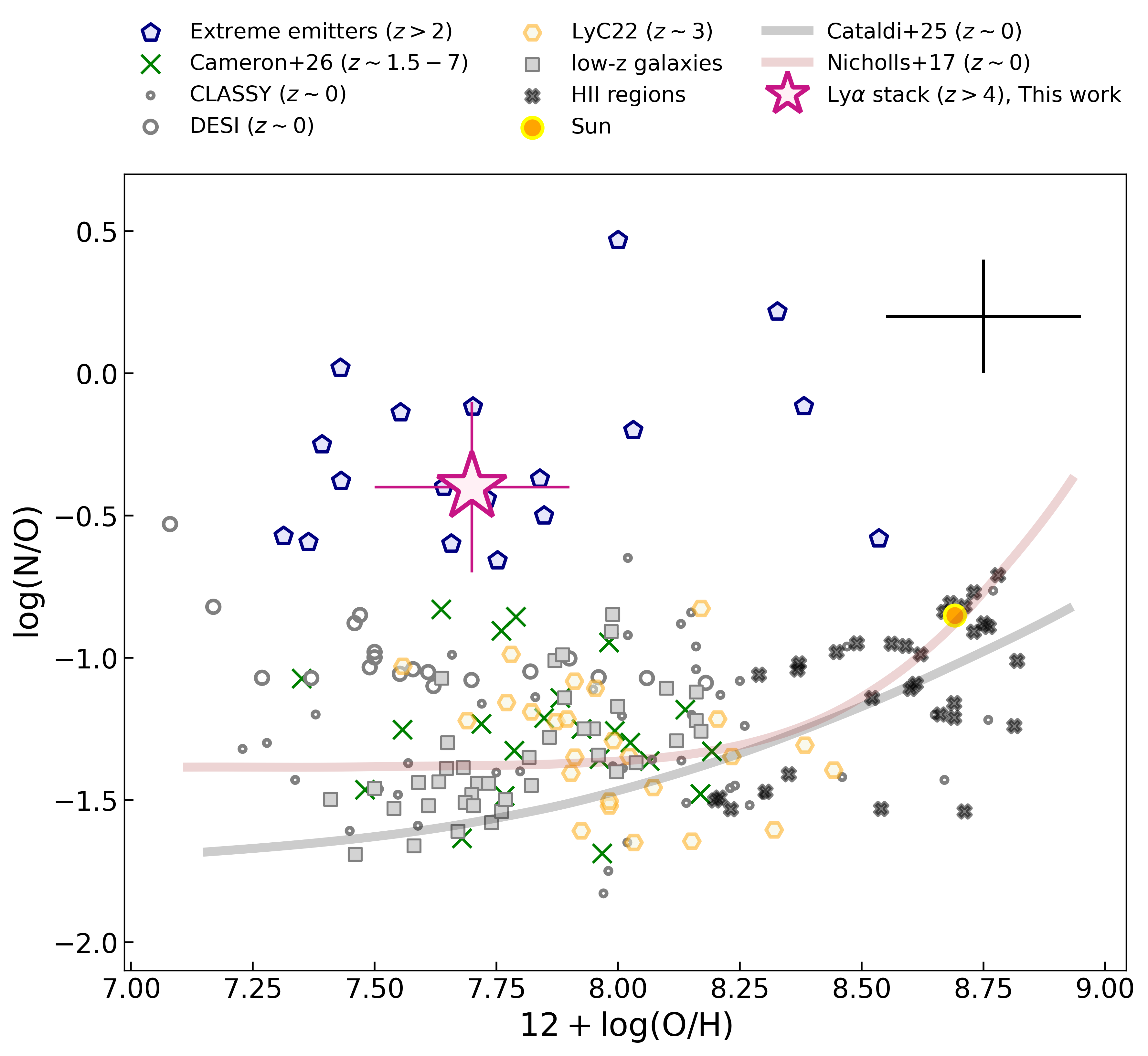
In Fig. 6, we compare the N/O abundance vs metallicity of our LAE stack with a compilation of nitrogen emitters spanning a wide range of redshifts (Schaerer et al., 2024; Topping et al., 2024; Castellano et al., 2024; Napolitano et al., 2025a; Zavala et al., 2024; Izotov et al., 2023; Cameron et al., 2026; Bhattacharya & Kobayashi, 2025; Arellano-Córdova et al., 2025; Isobe et al., 2023; Naidu et al., 2026; Martinez et al., 2025; Marques-Chaves et al., 2024). Interestingly, high N/O ratio has also been found in Haro 11, a system with both measured LyC and Ly$\alpha$ escape (James et al., 2013; Komarova et al., 2024). The average error on metallicity and N/O for the literature compilation is reported as black cross in the upper right corner of the plot. Our result is shown as a magenta star that conservatively accounts for uncertainties arising from the metallicity determination using different models, the spatial variation of metallicity within the stack (yielding $12+\log(\rm O/H)=7.7\pm 0.2$, see Sect. 5.2), and from the N/O determination using different relations and at different radii (yielding $\log(\rm N/O)=-0.4\pm 0.3$, see Sects. 4, 5.2). We find that LAEs exhibit enhanced nitrogen-over-oxygen abundance, which is comparable to that observed in other high-redshift star-forming galaxies. Although the available data prevent us from ascertaining the origin of the observed high N/O ratio, we explore two possible scenarios.

In recent years, mounting evidence has pointed to a growing population of nitrogen-enriched galaxies at high redshift, including both star-forming systems and AGN hosts (Schaerer et al., 2026; Cataldi et al., 2025; Curti et al., 2024; Napolitano et al., 2025a; Flury et al., 2025; Isobe et al., 2025; Tripodi et al., 2025; Ji et al., 2024; Rizzuti et al., 2025; Stiavelli et al., 2025; Topping et al., 2024; Zhu et al., 2025, 2026; Hayes et al., 2025). In particular, Cataldi et al. (2025) presented a comprehensive analysis of $\sim 500$ nitrogen emitters at $z\sim 2$–6, showing that high-redshift galaxies exhibit a systematic enhancement in N/O relative to the local relation, with $\Delta({\rm N/O})\sim 0.18$ dex on average. This enhancement is metallicity dependent, reaching $\sim 0.3$–0.4 dex at $12+\log(\rm O/H)\lesssim 8.1$. This turn-over point is, by definition, affected as well by the turn-over point from the N/O vs O/H relation, which changes slightly depending on the methodology used for the chemical abundance estimations (Vincenzo et al., 2016; Andrews & Martini, 2013; Pérez-Díaz et al., 2021). A similar picture emerges for AGN host galaxies: a stacking analysis of Type I and Type II AGN hosts at $z\sim 4$–7 reports elevated nitrogen abundances, with $\log(\rm N/O)>-0.6$ (Isobe et al., 2025). Nitrogen enhancement has been explained invoking several processes. For instance, it has been suggested that super star clusters containing Wolf-Rayet stars and massive stars ($M\gtrsim 10^{4}\penalty 10000\ \rm M_{\odot}$) are the most likely culprits of N-enhancement (Zhu et al., 2026). In detail, massive stars with low metallicity and high angular velocity may produce nitrogen in the first Myrs of their existence: the high rotation favors the transportation of the C into the core causing a bottleneck in the CNO cycle. This makes N destruction highly inefficient and, therefore, nitrogen accumulates and is easily ejected in the surrounding medium through stellar winds or stellar collapse (Meynet & Maeder, 2002; Zhu et al., 2026). Interestingly, some high-z ‘N-enhanced’ galaxies have also been interpreted as proto-clusters that would later evolve into globular clusters in the local universe (Cameron et al., 2023; Senchyna et al., 2024; Ji et al., 2025; Schaerer et al., 2025).

Alternatively, LAEs may display elevated N/O ratios due to oxygen depletion rather than nitrogen enrichment. Evidence of oxygen depletion has been found in a sample of infrared galaxies by Pérez-Díaz et al. (2024). Thanks to constraints on stellar mass, metallicity, star formation rate and N/O they were able to single out the origin on N/O enhancement finding that, for some galaxies, episodes of pristine gas infall due to mergers could have reduced the amount of oxygen, directly boosting the N/O ratio. Other works favour the interpretation of oxygen depletion caused by either supernova winds, dilution by pristine gas, or a combination of high star-formation and differential galactic winds (Stiavelli et al., 2025; McClymont et al., 2026; Rizzuti et al., 2025; Arroyo-Polonio et al., 2023).

Figure 9: Averaged radial profiles of the observed continuum UV slope (Top left), the rest-frame EW(Ly$\alpha$) (Top right), the escape fraction of Ly$\alpha$, $f_{\rm esc}^{\rm Ly\alpha}$ (Bottom left) and the gas-phase metallicity (Bottom right) compared with SPICE simulations with smooth and bursty stellar models.

5.4 Ly$\alpha$ properties and connection with UV-optical emission lines

The left and central panels of Fig. 7 show the averaged radial profiles of the equivalent widths (EWs) of Hα, Hβ, [O iii], C iii], and Ly$\alpha$. While the optical non-resonant emission lines display mild to steeply declining trends with increasing radius, the EW(Ly$\alpha$) exhibits a pronounced increase toward the outskirts. Since the EW traces the ratio between the considered line flux and adjacent continuum, we interpret the spatially increasing trend of EW(Ly$\alpha$) as a proof of spatially extended Ly$\alpha$ emission with respect to the compact UV-continuum due to resonant scattering (e.g., Kusakabe et al., 2022; Jung et al., 2024; Scholtz et al., 2024). Such a trend has also been observed in local Ly$\alpha$ emitters from the LaCOS survey, which consists of green pea-like galaxies around $z\sim 0.2$ (Saldana-Lopez et al., 2026). They found that the scale length of Ly$\alpha$ halos can be 10$\times$ larger than that in the UV, for that sample of starbursts.

Interestingly, the EW(C iii]) also increases in pixels $>0$ by a factor of 2, despite the fact that it is not a resonant line.

In star-forming galaxies, the EWs of Balmer recombination lines such as Hβ and Hα are known to trace the cosmic evolution of the specific star formation rate (sSFR; Fumagalli et al. 2012; Sobral et al. 2014). For a fixed stellar population age (see right panel of Fig. 7), EW$(\text{Hb})$ can therefore be used as a rough proxy for sSFR. In this context, the higher EW$(\text{Hb})$ observed in the central regions suggests that our sample is dominated by galaxies experiencing centrally concentrated star formation, leading to the rapid build-up of stellar mass in their inner regions (e.g., Baker et al. 2023; Dekel et al. 2009; Krumholz et al. 2018; Tacchella et al. 2016; Tripodi et al. 2023; Zolotov et al. 2015; see also Zhang et al. 2012 for a local dwarf galaxy analogue). A qualitatively similar, but even stronger, trend has been reported for stacked AGN host galaxies at $z>4$ (Tripodi et al., 2024). Although the upper limits on Hα in pixels $\pm 2$, due to the uncertain contribution of [N ii]λ6584, are consistent with this picture, the trend at these radii remains tentative given the large uncertainties on EW(Hβ).

Using our constraints on the Ly$\alpha$ and Hα fluxes, we can estimate the Ly$\alpha$ escape fraction ($f_{\rm esc}^{\rm Ly\alpha}$), defined as the ratio between the observed and intrinsic Ly$\alpha$ flux. The observed Hα flux serves as a proxy for the intrinsic Ly$\alpha$ emission under the assumption of Case B recombination and a null dust attenuation, such that

$$f^{\rm Ly\alpha}_{\rm esc}=\dfrac{F^{\rm Ly\alpha}_{\rm obs}}{F^{\rm Ly\alpha}_{\rm int}}=\dfrac{F^{\rm Ly\alpha}_{\rm obs}}{8.2\times F^{\text{Ha}}_{\rm obs}}.$$ (1)

Applying this relation at each radius, we find $f^{\rm Ly\alpha}_{\rm esc}\simeq 16\%$ in the central regions, increasing to $f^{\rm Ly\alpha}_{\rm esc}\gtrsim 24\%$ in the outskirts. The resulting averaged radial trend is shown in the bottom panel of Fig. 9. Comparable high Ly$\alpha$ escape fractions have been measured in individual LAEs at $z>6$ (Saxena et al., 2024; Napolitano et al., 2024; Llerena et al., 2025a), supporting the idea that our stacked sample is representative of the broader LAE population at $z>4$. Furthermore, the average $f^{\rm Ly\alpha}_{\rm esc}\gtrsim 20\%$ found in our stack is in agreement with the value derived from the empirical $f^{\rm Ly\alpha}_{\rm esc}-\mathrm{EW}(Ly\alpha)$ relation reported in (Saxena et al., 2024) at EW(Ly$\alpha$)=60Å, which matches the median EW(Ly$\alpha$)_median in our analysis. Since both Ly$\alpha$ and Hα originate from star-forming regions, the increasing trend of $f^{\rm Ly\alpha}_{\rm esc}$ as a function of the radial profile further supports our previous finding of a more spatially extended Ly$\alpha$ emission due to its resonant scattering process with respect to the non-resonant Balmer lines.

Finally, we estimate the ionizing photon production efficiency, $\xi_{\rm ion}$, using the EW([O iii]) as a proxy and adopting the empirical relation calibrated for star-forming galaxies at $z\sim 4$–10 by Llerena et al. (2025b). Averaged over all radii, we find $\log(\xi_{\rm ion}/{\rm Hz,erg^{-1}})\simeq 25.2\pm 0.1$, where the uncertainty includes systematic errors in the adopted calibration. This value lies close to the mean $\xi_{\rm ion}$ reported in the literature for galaxies with $M_{\rm UV}\simeq-19.1$ (Llerena et al., 2025b) and at $M_{\rm UV}\simeq-18,\penalty 10000\ 5<z<8$ (Papovich et al., 2025), in good agreement with the median UV magnitude of our sample, $M_{\rm UV,median}=-18.7$. Moreover, it agrees well with the values of $\xi_{\rm ion}$ inferred by semi-analytical model at $4<z<10$ (Yung et al., 2020).

5.5 The connection between UV-optical lines and LyC escape

Since the escape of Ly$\alpha$ and LyC photons is facilitated by similar interstellar medium geometries and low column densities (Verhamme et al., 2017), Ly$\alpha$ is widely considered an important tracer of Lyman continuum (LyC) escape. Indeed, several Ly$\alpha$ properties correlate with LyC escape, including the Ly$\alpha$ equivalent width, the Ly$\alpha$ escape fraction, and the Ly$\alpha$ velocity offset (Marchi et al., 2018; Verhamme et al., 2017).

Empirically, $f_{\rm esc}^{\rm Ly\alpha}\sim 20\%$ typically corresponds to $f_{\rm esc}^{\mathrm{LyC}}\sim 5$–$10\%$, with the latter generally smaller (e.g., Flury et al., 2022). The LaCOS resolved study of Ly$\alpha$ emission confirms correlations between Ly$\alpha$ EW and Ly$\alpha$ luminosity with $f_{\rm esc}^{\mathrm{LyC}}$ (Le Reste et al., 2025), although they also find an anticorrelation between Ly$\alpha$ halo size and $f_{\rm esc}^{\mathrm{LyC}}$ (Saldana-Lopez et al., 2026). But overall, our inferred Ly$\alpha$ escape fractions are compatible with moderate LyC leakage. Another proposed tracer of LyC escape is the [O iii]λλ4959,5007/[O ii]λλ3726,3729 ratio (O32; Jaskot & Oey 2013; Izotov et al. 2018). Although recent studies indicate that the correlation between O32 and $f_{\rm esc}^{\mathrm{LyC}}$ is not tight—likely due to complex gas geometry and kinematics—a high O32 appears to be a necessary (though not sufficient) condition for significant leakage (e.g., as shown for Haro 11 by Keenan et al., 2017). For instance, Flury et al. (2022) showed that among galaxies with $\log(\mathrm{O32})>1.0$, more than 60% are strong LyC leakers ($f_{\rm esc}^{\mathrm{LyC}}>5\%$). Our stacked spectra show $\log(\mathrm{O32})>1.0$ at all radii except for pix$=-2$, where $\log(\mathrm{O32})=0.86\pm 0.05$ (Tab. 3), further supporting the picture of density-bounded or porous ionized regions.

We can also estimate $f_{\rm esc}^{\mathrm{LyC}}$ from the relation between the UV continuum slope and LyC escape fraction derived by Chisholm et al. (2022) and calibrated using the LzLCS survey (Jaskot et al., 2024). Applying this relation to our radial $\beta_{\rm UV}$ measurements yields $f_{\rm esc}^{\mathrm{LyC}}\sim 3\%$ in the central regions, increasing up to $\sim 15\%$ in the outskirts, in broad agreement with the indirect constraints discussed above. Finally, Schaerer et al. (2022) suggested that strong LyC leakers typically exhibit $\text{{C}\,{\sc{iv}}{}{}{}{}}/\text{{C}\,{\sc{iii}}]{}{}{}{}}\gtrsim 0.75$ (see also Saxena et al. 2022). In our data, C iv is securely detected only in pixels $0$ and $1$, limiting the applicability of this diagnostic across all radii. Nevertheless, the measured ratios are consistent with moderate LyC escape rather than extreme leakage ($f_{\rm esc}^{\mathrm{LyC}}>0.1$) that would be expected from the observed C iv/C iii] compared with the threshold defined by Schaerer et al. (2022), as shown in Fig. 8. Moreover, we find $f_{\rm esc}^{\mathrm{LyC}}<f^{\rm Ly\alpha}_{\rm esc}$, which is consistent with the results reported in (Saxena et al., 2024). By means of the same diagnostic plot, our stack is also classified as star-forming lying below the empirical AGN threshold.

Overall, the combined UV line ratios, O32 values, $\beta_{\rm UV}$ trends, and Ly$\alpha$ escape fractions—consistently indicate that our LAEs are dominated by stellar photoionization and likely exhibit moderate LyC escape fractions. These properties reinforce the scenario in which typical $z>4$ LAEs represent efficient, though not extreme, contributors to the ionizing photon budget during cosmic reionization.

6 Constraining feedback models from the SPICE simulations

In this section, we compare some observed properties of our LAEs stack with predictions from the SPICE simulations. As shown in Bhagwat et al. (2024), variations in supernova feedback significantly influence the strength of galactic outflows. These differences reshape the interstellar and circumgalactic media, thereby affecting the escape fraction of Lyman-continuum photons and leading to distinct reionization scenarios. The SPICE radiation-hydrodynamic simulations account for two different modes of supernova feedback, namely smooth and bursty (Bhagwat et al., 2024, 2025). The difference in the models originates from the timing of injection of supernova energy leading to highly stochastic star-formation histories in the bursty model, while non-stochastic star-formation in the smooth model (Basu et al., 2026). To enable a proper comparison with our observed properties, we built a simulated stacked sample, which comprises 132 Ly$\alpha$ emitters per feedback model in a range of redshift and UV magnitude matching the observed ones. For each LAE, we extracted datacubes in 12 random line-of-sight (los). Then, for each galaxy and los, we placed 5 JWST/NIRSpec mock slits at different inclination angles, all centered on the peak of UV emission. This results in a total of 132$\times$12$\times$5 simulated spectra per feedback model. For each model, we stacked all the generated 2D spectra adopting the same procedure as the observed stack (see Sect. 3). Finally, the UV continuum slope, and the EW of Ly$\alpha$, Hα and Hβ are calculated using the stacked spectra.

In the top and bottom panels of Fig. 9, we compare the radial profiles of the UV continuum slope, rest-frame EW(Ly$\alpha$), Ly$\alpha$ escape fraction and metallicity with the results from the SPICE models. The SPICE bursty model produces bluer UV slopes than the smooth model and therefore matches our observations more closely. In both SPICE smooth and bursty models, the EW(Ly$\alpha$) and Ly$\alpha$ escape fractions increase with radius. However, the bursty model shows a significantly stronger rise, particularly in the second radial bin (pixel 2), where both the EW(Ly$\alpha$) and Ly$\alpha$ escape fraction increase sharply relative to the central bin. Conversely, the smooth model predicts a more gradual increase with a smaller amplitude for EW(Ly$\alpha$) and a flattening for the Ly$\alpha$ escape fraction. In SPICE, the enhanced rise shown by the bursty case is associated with feedback driven outflows that reduce central H I column densities and create low-density channels (see Bhagwat et al., 2024). These ISM conditions increase the escape probability of resonantly scattered Ly$\alpha$ photons and redistribute them outward relative to the UV continuum. The smooth model instead maintains higher and more centrally concentrated neutral gas columns, leading to lower Ly$\alpha$ escape fractions and weaker radial variation.

The Balmer line EW profiles provide an independent constraint. Under Case B recombination, Hα and Hβ originate from the same H II regions and trace the same emission measure, with a fixed intrinsic ratio (Osterbrock & Ferland, 2006). Therefore, in the absence of dust, their radial profiles should have identical shapes up to a constant factor. While the observed radial profiles of Hα and Hβ equivalent width match and are consistent with negligible dust (see Fig. 7), in the smooth model we find that EW(Hα) decreases with radius, but less steeply than EW(Hβ). Indeed, the smooth model shows a centrally enhanced dust density, thus suppressing Hβ more strongly and steepening its radial EW profile relative to Hα.

Finally, the metallicity profiles predicted by SPICE (Garcia et al., 2025b, a) are also strongly affected by the feedback model (bottom right panel of Fig. 9). The smooth model develops a steep negative metallicity gradient with elevated central metallicities, which is also connected to the stronger central dust attenuation (see Bhagwat et al., 2024) and higher attenuation of Hβ. Conversely, the bursty model exhibits flatter and overall lower metallicity profiles in agreement with our observed profiles, implying a combination of the redistribution of metal-enriched gas by episodic feedback and inside-out growth. The weaker radial dust gradients in this model also produce more similar EW radial profiles for Hα and Hβ.

Overall, we have demonstrated that comparing synthetic SPICE observables with real data provides a powerful approach to disentangling and constraining different feedback mechanisms at high redshift. Specifically, the combined radial trends in EW(Ly$\alpha$) and Ly$\alpha$ escape fraction, particularly the pronounced rise at intermediate radii, together with flatter metallicity gradients and moderate Balmer EW slopes, indicate that the bursty SPICE feedback prescription is in agreement with the data presented and thus highly favored.

Such a model naturally provides for a more bursty star formation history, which has been proposed as a potential explanation for the high abundance of luminous sources observed at early cosmic times (e.g., Gelli et al., 2024; Muñoz et al., 2026). However, within the SPICE simulations, the dust-attenuated luminosity functions predicted by both the bursty and smooth feedback models reproduce observations equally well up to $z=10$ (Bhagwat et al., 2024). This degeneracy suggests that additional constraints are required. In particular, comparisons with other observables, such as galaxy morphology and kinematics, could provide further discriminatory power.

7 Summary and Conclusions

In this work, we performed a spatially resolved stacked analysis of 287 LAEs at $z>4$ using JWST/NIRSpec prism spectroscopy. Specifically, we investigated the radial trend of emission lines and continuum properties on sub-kiloparsec scales. Our main findings can be summarized as follows:

• LAEs exhibit strong UV and optical emission lines, including Ly$\alpha$, C III], [O II], [Ne III], Balmer lines, and [O iii] across multiple spatial elements. High-ionization features such as C iv and He II are confined to the central regions, suggesting stratified ionization conditions.

• Radially increasing blue UV slopes ($\beta_{\rm UV}\sim-2.2$ on average) and Balmer decrements consistent with Case B recombination indicate negligible dust attenuation at all radii.

• Using $T_{e}$-based measurements, HCm, and photoionization models, we consistently derive sub-solar metallicities of $\sim 10$–15% $Z_{\odot}$ ($12+\log({\rm O/H})\sim 7.5$–7.9). We find evidence for either a negative (i.e. decreasing) or flat metallicity gradient with radius. The ionization parameter is high, $\log(U)\sim-1.5$ in the central regions, mildly decreasing outward, and the gas density is consistent with $\log(n/{\rm cm}^{-3})\sim 3$.

• We measure elevated nitrogen-to-oxygen ratios ($\log({\rm N/O})\sim-0.4\pm 0.3$), placing LAEs among the growing population of nitrogen-enriched galaxies at high redshift.

• While non-resonant optical lines show declining equivalent-width profiles with radius, EW(Ly$\alpha$) increases toward the outskirts, indicating spatially extended Ly$\alpha$ emission relative to the UV continuum. The Ly$\alpha$ escape fraction rises from $\sim 16\%$ in the center to $\gtrsim 24\%$ in the outer regions.

• We infer $\log(\xi_{\rm ion}/{\rm Hz\,erg^{-1}})\simeq 25.2\pm 0.1$, consistent with galaxies of similar UV luminosity and supportive of efficient ionizing photon production.

• Comparison with SPICE radiation-hydrodynamic simulations favors bursty supernova feedback models, which better reproduce the observed radial trends of EW(Ly$\alpha$) and $f_{\rm esc}^{\rm Ly\alpha}$.

Overall, our analysis demonstrates that Ly$\alpha$ emission is not merely a tracer of instantaneous star formation, but a sensitive probe of the internal structure, feedback processes, and circumgalactic environment of early galaxies. The increasing Ly$\alpha$ escape fraction with radius supports a scenario in which resonant scattering redistributes Ly$\alpha$ photons into lower-density outer regions, where they can escape more efficiently. These properties suggest that typical $z>4$ LAEs are efficient, though not extreme, contributors to the ionizing photon budget during cosmic reionization.

Importantly, our stacked analysis probes the bulk of the LAE population at $z_{\rm median}=5.5$, characterized by $M_{\rm UV,median}=-18.7$ and EW(Ly$\alpha$)_median=61 Å, rather than rare, exceptionally luminous systems. Our results therefore provide a representative view of the physical conditions and Ly$\alpha$ radiative transfer properties in typical high-redshift LAEs.

More broadly, this work highlights the power of stacked JWST spectroscopy to deliver a population-level view of the internal structure of early galaxies that would otherwise remain inaccessible. By statistically resolving radial trends in emission-line and continuum properties, stacking bridges the gap between detailed studies of rare bright systems and the average properties of the high-redshift galaxy population. As JWST surveys continue to expand and the number of spectroscopically confirmed LAEs increases, this approach will enable us to explore how Ly$\alpha$ emission, metallicity, ionization conditions, and escape fractions depend on $M_{\rm UV}$, redshift, and EW(Ly$\alpha$), providing a more comprehensive framework for understanding the role of LAEs during the first billion years of cosmic history.

Appendix A Spectra for off-centered pixels

Figure 10: Same as Fig. 3 for pixels 1 and -1 of the LAEs stack.

Figure 11: Same as Fig. 3 for pixels 2 and -2 of the LAEs stack.

In Fig. 10-11, we show the spectra extracted from the off-centered pixels (pixels 1,-1,2,-2).

Appendix B Comparison of the models with and without the [N II] component

In Fig. 12, we compare the best-fitting models of the blended Hα –[N ii]λλ6548,6584 feature obtained without (top panel) and with (bottom panel) the inclusion of the [N II] component. The observed spectrum clearly favors the model including the [N II] doublet, as it accounts for the excess flux on the blue side of Hα and yields a significant improvement in the Bayesian Information Criterion (BIC).

Figure 12: Comparison of the best-fitting models of the blended Hα-[N ii]λλ6548,6584 without (top) and with (bottom) the [N II] component.

Appendix C OHNO diagram with conservative blending correction for [Ne iii]

In Fig. 13 we show the [Ne iii]/[O ii] ratio corrected for the blending contamination along with the uncorrected ratios and the photoionization models, already presented in Fig. 5.

Figure 13: Same as the right panel of Fig. 5 but with the [Ne iii]/[O ii] ratio corrected for the blending contamination as lighter circles. The maximum correction for [Ne iii]λ3869 due to the blend with He i λ3889, Hη and Hζ is $\approx$ 0.3 dex.

Appendix D Table

In Tab. 3 we report the line ratios used in Sects. 4.4, 4.2 to estimate the contamination correction for [Ne iii] _blend and the contribution of [N ii]λ6584 to Hα, respectively.

Table 3: Line ratios

Line ratio	Pix -2	Pix -1	Pix 0	Pix 1	Pix 2
Hδ/[Ne iii] blend	$0.42\pm 0.20$	$0.34\pm 0.04$	$0.37\pm 0.03$	$0.30\pm 0.04$	$0.34\pm 0.10$
Hη/[Ne iii] blend	$0.11\pm 0.04$	$0.10\pm 0.01$	$0.10\pm 0.01$	$0.08\pm 0.01$	$0.10\pm 0.02$
Hζ/[Ne iii] blend	$0.17\pm 0.05$	$0.14\pm 0.02$	$0.15\pm 0.01$	$0.12\pm 0.02$	$0.14\pm 0.04$
He i λ3889/[Ne iii] blend	N/A	$0.24\pm 0.03$	$0.20\pm 0.02$	$0.17\pm 0.03$	N/A
[Ne iii]λ3869/[Ne iii] blend	$<0.7$	$0.52\pm 0.06$	$0.55\pm 0.04$	$0.63\pm 0.06$	$<0.8$
[N ii]λ6584/Hα	N/A	$0.10\pm 0.05$	$0.10\pm 0.02$	$0.17\pm 0.05$	N/A
[O iii]λλ4959,5007/[O ii]λλ3726,3729	$12_{-2}^{+3}$	$11\pm 1$	$15\pm 1$	$12\pm 1$	$7\pm 1$

Notes. Columns: ratios name; values of line ratio in different pixels from -2 to 2, assuming no dust correction.

References

- Andrews & Martini (2013) Andrews, B. H. & Martini, P. 2013, ApJ, 765, 140
- Arellano-Córdova et al. (2025) Arellano-Córdova, K. Z., Berg, D. A., Mingozzi, M., et al. 2025, MNRAS, 544, 1588
- Arevalo-Gonzalez et al. (2025) Arevalo-Gonzalez, F., Tripodi, R., Llerena, M., et al. 2025, arXiv e-prints, arXiv:2512.16365
- Arrabal Haro et al. (2023) Arrabal Haro, P., Dickinson, M., Finkelstein, S. L., et al. 2023, ApJ, 951, L22
- Arroyo-Polonio et al. (2023) Arroyo-Polonio, A., Iglesias-Páramo, J., Kehrig, C., et al. 2023, A&A, 677, A114
- Asplund et al. (2021) Asplund, M., Amarsi, A. M., & Grevesse, N. 2021, A&A, 653, A141
- Backhaus et al. (2022) Backhaus, B. E., Trump, J. R., Cleri, N. J., et al. 2022, ApJ, 926, 161
- Backhaus et al. (2024) Backhaus, B. E., Trump, J. R., Pirzkal, N., et al. 2024, ApJ, 962, 195
- Baker et al. (2023) Baker, W. M., Tacchella, S., Johnson, B. D., et al. 2023, arXiv e-prints, arXiv:2306.02472
- Basu et al. (2026) Basu, A., Bhagwat, A., Ciardi, B., & Costa, T. 2026, MNRAS, 545, staf2240
- Berg et al. (2016) Berg, D. A., Skillman, E. D., Henry, R. B. C., Erb, D. K., & Carigi, L. 2016, ApJ, 827, 126
- Bhagwat et al. (2024) Bhagwat, A., Costa, T., Ciardi, B., Pakmor, R., & Garaldi, E. 2024, MNRAS, 531, 3406
- Bhagwat et al. (2025) Bhagwat, A., Napolitano, L., Pentericci, L., Ciardi, B., & Costa, T. 2025, MNRAS, 542, 128
- Bhattacharya & Kobayashi (2025) Bhattacharya, S. & Kobayashi, C. 2025, arXiv e-prints, arXiv:2508.11998
- Böker et al. (2023) Böker, T., Beck, T. L., Birkmann, S. M., et al. 2023, PASP, 135, 038001
- Bouwens et al. (2014) Bouwens, R. J., Illingworth, G. D., Oesch, P. A., et al. 2014, ApJ, 793, 115
- Brinchmann (2023) Brinchmann, J. 2023, MNRAS, 525, 2087
- Byrne et al. (2022) Byrne, C. M., Stanway, E. R., Eldridge, J. J., McSwiney, L., & Townsend, O. T. 2022, MNRAS, 512, 5329
- Calzetti et al. (1994) Calzetti, D., Kinney, A. L., & Storchi-Bergmann, T. 1994, ApJ, 429, 582
- Cameron et al. (2026) Cameron, A. J., Carreira, C., Simmonds, C., et al. 2026, arXiv e-prints, arXiv:2601.15964
- Cameron et al. (2023) Cameron, A. J., Saxena, A., Bunker, A. J., et al. 2023, arXiv e-prints, arXiv:2302.04298
- Campbell et al. (1986) Campbell, A., Terlevich, R., & Melnick, J. 1986, MNRAS, 223, 811
- Carniani et al. (2024) Carniani, S., Venturi, G., Parlanti, E., et al. 2024, A&A, 685, A99
- Castellano et al. (2024) Castellano, M., Napolitano, L., Fontana, A., et al. 2024, ApJ, 972, 143
- Castellano et al. (2025) Castellano, M., Napolitano, L., Moreschini, B., et al. 2025, arXiv e-prints, arXiv:2512.08490
- Cataldi et al. (2025) Cataldi, E., Belfiore, F., Curti, M., et al. 2025, arXiv e-prints, arXiv:2512.07955
- Chisholm et al. (2022) Chisholm, J., Saldana-Lopez, A., Flury, S., et al. 2022, MNRAS, 517, 5104
- Cullen et al. (2023) Cullen, F., McLure, R. J., McLeod, D. J., et al. 2023, MNRAS, 520, 14
- Curti et al. (2024) Curti, M., Maiolino, R., Curtis-Lake, E., et al. 2024, A&A, 684, A75
- Curtis-Lake et al. (2025a) Curtis-Lake, E., Cameron, A. J., Bunker, A. J., et al. 2025a, arXiv e-prints, arXiv:2510.01033
- Curtis-Lake et al. (2025b) Curtis-Lake, E., Cameron, A. J., Bunker, A. J., et al. 2025b, arXiv e-prints, arXiv:2510.01033
- Davis et al. (2007) Davis, M., Guhathakurta, P., Konidaris, N. P., et al. 2007, ApJ, 660, L1
- de Graaff et al. (2025) de Graaff, A., Brammer, G., Weibel, A., et al. 2025, A&A, 697, A189
- Dekel et al. (2009) Dekel, A., Sari, R., & Ceverino, D. 2009, ApJ, 703, 785
- Dottorini et al. (2025) Dottorini, D., Calabrò, A., Pentericci, L., et al. 2025, A&A, 698, A234
- Finkelstein et al. (2012) Finkelstein, S. L., Papovich, C., Salmon, B., et al. 2012, ApJ, 756, 164
- Flury et al. (2025) Flury, S. R., Arellano-Córdova, K. Z., Moran, E. C., & Einsig, A. 2025, MNRAS, 543, 3367
- Flury et al. (2022) Flury, S. R., Jaskot, A. E., Ferguson, H. C., et al. 2022, ApJ, 930, 126
- Foreman-Mackey et al. (2013) Foreman-Mackey, D., Hogg, D. W., Lang, D., & Goodman, J. 2013, PASP, 125, 306
- Fujimoto et al. (2025) Fujimoto, S., Faisst, A. L., Tsujita, A., et al. 2025, arXiv e-prints, arXiv:2510.16116
- Fumagalli et al. (2012) Fumagalli, M., Patel, S. G., Franx, M., et al. 2012, ApJ, 757, L22
- Garcia et al. (2025a) Garcia, A. M., Torrey, P., Bhagwat, A., et al. 2025a, Metallicity Gradients in Modern Cosmological Simulations II: The Role of Bursty Versus Smooth Feedback at High-Redshift
- Garcia et al. (2025b) Garcia, A. M., Torrey, P., Bhagwat, A., et al. 2025b, Metallicity Gradients in Modern Cosmological Simulations I: Tension Between Smooth Stellar Feedback Models and Observations
- Gardner et al. (2023) Gardner, J. P., Mather, J. C., Abbott, R., et al. 2023, PASP, 135, 068001
- Gardner et al. (2006) Gardner, J. P., Mather, J. C., Clampin, M., et al. 2006, Space Sci. Rev., 123, 485
- Gelli et al. (2024) Gelli, V., Mason, C., & Hayward, C. C. 2024, ApJ, 975, 192
- Grogin et al. (2011) Grogin, N. A., Kocevski, D. D., Faber, S. M., et al. 2011, ApJS, 197, 35
- Gunasekera et al. (2025) Gunasekera, C. M., van Hoof, P. A. M., Dehghanian, M., et al. 2025, arXiv e-prints, arXiv:2508.01102
- Hayes et al. (2014) Hayes, M., Östlin, G., Duval, F., et al. 2014, ApJ, 782, 6
- Hayes et al. (2025) Hayes, M. J., Saldana-Lopez, A., Citro, A., et al. 2025, ApJ, 982, 14
- Heintz et al. (2024) Heintz, K. E., Watson, D., Brammer, G., et al. 2024, Science, 384, 890
- Hu et al. (2024) Hu, W., Papovich, C., Dickinson, M., et al. 2024, ApJ, 971, 21
- Inoue et al. (2020) Inoue, A. K., Yamanaka, S., Ouchi, M., et al. 2020, PASJ, 72, 101
- Isobe et al. (2025) Isobe, Y., Maiolino, R., D’Eugenio, F., et al. 2025, MNRAS, 541, L71
- Isobe et al. (2023) Isobe, Y., Ouchi, M., Tominaga, N., et al. 2023, ApJ, 959, 100
- Izotov et al. (2023) Izotov, Y. I., Schaerer, D., Worseck, G., et al. 2023, MNRAS, 522, 1228
- Izotov et al. (2018) Izotov, Y. I., Worseck, G., Schaerer, D., et al. 2018, MNRAS, 478, 4851
- Jakobsen et al. (2022) Jakobsen, P., Ferruit, P., Alves de Oliveira, C., et al. 2022, A&A, 661, A80
- James et al. (2013) James, B. L., Tsamis, Y. G., Walsh, J. R., Barlow, M. J., & Westmoquette, M. S. 2013, MNRAS, 430, 2097
- Jaskot & Oey (2013) Jaskot, A. E. & Oey, M. S. 2013, ApJ, 766, 91
- Jaskot et al. (2024) Jaskot, A. E., Silveyra, A. C., Plantinga, A., et al. 2024, ApJ, 973, 111
- Ji et al. (2025) Ji, X., Maiolino, R., Ferland, G., et al. 2025, MNRAS, 541, 2134
- Ji et al. (2024) Ji, X., Übler, H., Maiolino, R., et al. 2024, MNRAS, 535, 881
- Jones et al. (2025) Jones, G. C., Bunker, A. J., Saxena, A., et al. 2025, MNRAS, 536, 2355
- Jones et al. (2024) Jones, G. C., Bunker, A. J., Saxena, A., et al. 2024, A&A, 683, A238
- Jung et al. (2024) Jung, I., Finkelstein, S. L., Arrabal Haro, P., et al. 2024, ApJ, 967, 73
- Juodžbalis et al. (2026) Juodžbalis, I., Maiolino, R., Baker, W. M., et al. 2026, MNRAS[arXiv:2504.03551]
- Kageura et al. (2025) Kageura, Y., Ouchi, M., Nakane, M., et al. 2025, ApJS, 278, 33
- Katz et al. (2023) Katz, H., Saxena, A., Cameron, A. J., et al. 2023, MNRAS, 518, 592
- Keenan et al. (2017) Keenan, R. P., Oey, M. S., Jaskot, A. E., & James, B. L. 2017, ApJ, 848, 12
- Koekemoer et al. (2011) Koekemoer, A. M., Faber, S. M., Ferguson, H. C., et al. 2011, ApJS, 197, 36
- Komarova et al. (2024) Komarova, L., Oey, M. S., Hernandez, S., et al. 2024, ApJ, 967, 117
- Kornei et al. (2010) Kornei, K. A., Shapley, A. E., Erb, D. K., et al. 2010, ApJ, 711, 693
- Krumholz et al. (2018) Krumholz, M. R., Burkhart, B., Forbes, J. C., & Crocker, R. M. 2018, MNRAS, 477, 2716
- Kumari et al. (2024) Kumari, N., Smit, R., Witstok, J., et al. 2024, arXiv e-prints, arXiv:2406.11997
- Kusakabe et al. (2022) Kusakabe, H., Verhamme, A., Blaizot, J., et al. 2022, A&A, 660, A44
- Lawrence et al. (2007) Lawrence, A., Warren, S. J., Almaini, O., et al. 2007, MNRAS, 379, 1599
- Le Reste et al. (2025) Le Reste, A., Scarlata, C., Hayes, M. J., et al. 2025, ApJS, 280, 27
- Leclercq et al. (2017) Leclercq, F., Bacon, R., Wisotzki, L., et al. 2017, A&A, 608, A8
- Li et al. (2025) Li, Z., Cai, Z., Wang, X., et al. 2025, ApJS, 280, 62
- Llerena et al. (2025a) Llerena, M., Pentericci, L., Amorín, R., et al. 2025a, arXiv e-prints, arXiv:2510.25647
- Llerena et al. (2025b) Llerena, M., Pentericci, L., Napolitano, L., et al. 2025b, A&A, 698, A302
- Maiolino et al. (2024a) Maiolino, R., Scholtz, J., Witstok, J., et al. 2024a, Nature, 627, 59
- Maiolino et al. (2024b) Maiolino, R., Übler, H., Perna, M., et al. 2024b, A&A, 687, A67
- Marchi et al. (2018) Marchi, F., Pentericci, L., Guaita, L., et al. 2018, A&A, 614, A11
- Marques-Chaves et al. (2024) Marques-Chaves, R., Schaerer, D., Kuruvanthodi, A., et al. 2024, A&A, 681, A30
- Martinez et al. (2025) Martinez, Z., Berg, D. A., James, B. L., et al. 2025, ApJ, 995, 204
- Matthee et al. (2022) Matthee, J., Naidu, R. P., Pezzulli, G., et al. 2022, MNRAS, 512, 5960
- McClymont et al. (2026) McClymont, W., Tacchella, S., Smith, A., et al. 2026, MNRAS[arXiv:2507.08787]
- Meynet & Maeder (2002) Meynet, G. & Maeder, A. 2002, A&A, 390, 561
- Muñoz et al. (2026) Muñoz, J. B., Chisholm, J., Sun, G., et al. 2026, arXiv e-prints, arXiv:2601.07912
- Naidu et al. (2026) Naidu, R. P., Oesch, P. A., Brammer, G., et al. 2026, The Open Journal of Astrophysics, 9, 56033
- Nanayakkara et al. (2024) Nanayakkara, T., Glazebrook, K., Jacobs, C., et al. 2024, Scientific Reports, 14, 3724
- Napolitano et al. (2025a) Napolitano, L., Castellano, M., Pentericci, L., et al. 2025a, ApJ, 989, 75
- Napolitano et al. (2023) Napolitano, L., Pentericci, L., Calabrò, A., et al. 2023, A&A, 677, A138
- Napolitano et al. (2025b) Napolitano, L., Pentericci, L., Dickinson, M., et al. 2025b, arXiv e-prints, arXiv:2508.14171
- Napolitano et al. (2024) Napolitano, L., Pentericci, L., Santini, P., et al. 2024, A&A, 688, A106
- Nicholls et al. (2017) Nicholls, D. C., Sutherland, R. S., Dopita, M. A., Kewley, L. J., & Groves, B. A. 2017, MNRAS, 466, 4403
- Oke & Gunn (1983) Oke, J. B. & Gunn, J. E. 1983, ApJ, 266, 713
- Ono et al. (2010) Ono, Y., Ouchi, M., Shimasaku, K., et al. 2010, ApJ, 724, 1524
- Osterbrock & Ferland (2006) Osterbrock, D. E. & Ferland, G. J. 2006, Astrophysics of gaseous nebulae and active galactic nuclei
- Pahl et al. (2024) Pahl, A., Shapley, A., Steidel, C. C., et al. 2024, ApJ, 974, 212
- Papovich et al. (2025) Papovich, C., Cole, J. W., Hu, W., et al. 2025, arXiv e-prints, arXiv:2505.08870
- Pentericci et al. (2018) Pentericci, L., Vanzella, E., Castellano, M., et al. 2018, A&A, 619, A147
- Pérez-Díaz et al. (2021) Pérez-Díaz, B., Masegosa, J., Márquez, I., & Pérez-Montero, E. 2021, MNRAS, 505, 4289
- Pérez-Díaz et al. (2022) Pérez-Díaz, B., Pérez-Montero, E., Fernández-Ontiveros, J. A., & Vílchez, J. M. 2022, A&A, 666, A115
- Pérez-Díaz et al. (2024) Pérez-Díaz, B., Pérez-Montero, E., Fernández-Ontiveros, J. A., Vílchez, J. M., & Amorín, R. 2024, Nature Astronomy, 8, 368
- Pérez-Montero (2014) Pérez-Montero, E. 2014, MNRAS, 441, 2663
- Pérez-Montero (2017) Pérez-Montero, E. 2017, PASP, 129, 043001
- Pérez-Montero & Amorín (2017) Pérez-Montero, E. & Amorín, R. 2017, MNRAS, 467, 1287
- Pérez-Montero et al. (2021) Pérez-Montero, E., Amorín, R., Sánchez Almeida, J., et al. 2021, MNRAS, 504, 1237
- Pérez-Montero & Contini (2009) Pérez-Montero, E. & Contini, T. 2009, MNRAS, 398, 949
- Pérez-Montero et al. (2019) Pérez-Montero, E., Dors, O. L., Vílchez, J. M., et al. 2019, MNRAS, 489, 2652
- Pérez-Montero et al. (2020) Pérez-Montero, E., Kehrig, C., Vílchez, J. M., et al. 2020, A&A, 643, A80
- Planck Collaboration et al. (2020) Planck Collaboration, Aghanim, N., Akrami, Y., et al. 2020, A&A, 641, A6
- Prieto-Lyon et al. (2025) Prieto-Lyon, G., Mason, C. A., Strait, V., et al. 2025, arXiv e-prints, arXiv:2509.18302
- Reddy et al. (2015) Reddy, N. A., Kriek, M., Shapley, A. E., et al. 2015, ApJ, 806, 259
- Rizzuti et al. (2025) Rizzuti, F., Matteucci, F., Molaro, P., Cescutti, G., & Maiolino, R. 2025, A&A, 697, A96
- Roberts-Borsani et al. (2024) Roberts-Borsani, G., Treu, T., Shapley, A., et al. 2024, ApJ, 976, 193
- Saldana-Lopez et al. (2026) Saldana-Lopez, A., Hayes, M. J., Le Reste, A., et al. 2026, ApJ, 999, 71
- Sanders et al. (2025) Sanders, R. L., Shapley, A. E., Topping, M. W., et al. 2025, arXiv e-prints, arXiv:2508.10099
- Sandles et al. (2024) Sandles, L., D’Eugenio, F., Maiolino, R., et al. 2024, A&A, 691, A305
- Saxena et al. (2024) Saxena, A., Bunker, A. J., Jones, G. C., et al. 2024, A&A, 684, A84
- Saxena et al. (2022) Saxena, A., Cryer, E., Ellis, R. S., et al. 2022, MNRAS, 517, 1098
- Schaerer et al. (2026) Schaerer, D., Izotov, Y. I., Marques-Chaves, R., et al. 2026, arXiv e-prints, arXiv:2601.06968
- Schaerer et al. (2022) Schaerer, D., Izotov, Y. I., Worseck, G., et al. 2022, A&A, 658, L11
- Schaerer et al. (2025) Schaerer, D., Marques-Chaves, R., Atek, H., et al. 2025, arXiv e-prints, arXiv:2512.16549
- Schaerer et al. (2024) Schaerer, D., Marques-Chaves, R., Xiao, M., & Korber, D. 2024, A&A, 687, L11
- Schmidt et al. (2021) Schmidt, K. B., Kerutt, J., Wisotzki, L., et al. 2021, A&A, 654, A80
- Scholtz et al. (2024) Scholtz, J., Witten, C., Laporte, N., et al. 2024, A&A, 687, A283
- Scoville et al. (2007) Scoville, N., Aussel, H., Brusa, M., et al. 2007, ApJS, 172, 1
- Senchyna et al. (2024) Senchyna, P., Plat, A., Stark, D. P., et al. 2024, ApJ, 966, 92
- Shapley et al. (2023) Shapley, A. E., Reddy, N. A., Sanders, R. L., Topping, M. W., & Brammer, G. B. 2023, ApJ, 950, L1
- Sobral et al. (2014) Sobral, D., Best, P. N., Smail, I., et al. 2014, MNRAS, 437, 3516
- Steidel et al. (2011) Steidel, C. C., Bogosavljević, M., Shapley, A. E., et al. 2011, ApJ, 736, 160
- Steidel et al. (2016) Steidel, C. C., Strom, A. L., Pettini, M., et al. 2016, ApJ, 826, 159
- Stiavelli et al. (2025) Stiavelli, M., Morishita, T., Chiaberge, M., et al. 2025, ApJ, 981, 136
- Storey & Hummer (1995) Storey, P. J. & Hummer, D. G. 1995, MNRAS, 272, 41
- Tacchella et al. (2016) Tacchella, S., Dekel, A., Carollo, C. M., et al. 2016, MNRAS, 458, 242
- Tang et al. (2023) Tang, M., Stark, D. P., Chen, Z., et al. 2023, MNRAS, 526, 1657
- Tang et al. (2024) Tang, M., Stark, D. P., Ellis, R. S., et al. 2024, MNRAS, 531, 2701
- Taylor et al. (2025) Taylor, A. J., Kokorev, V., Kocevski, D. D., et al. 2025, ApJ, 989, L7
- Topping et al. (2024) Topping, M. W., Stark, D. P., Senchyna, P., et al. 2024, MNRAS, 529, 3301
- Tripodi et al. (2024) Tripodi, R., D’Eugenio, F., Maiolino, R., et al. 2024, A&A, 692, A184
- Tripodi et al. (2023) Tripodi, R., Lelli, F., Feruglio, C., et al. 2023, A&A, 671, A44
- Tripodi et al. (2025) Tripodi, R., Martis, N., Markov, V., et al. 2025, Nature Communications, 16, 9830
- Trussler et al. (2023) Trussler, J. A. A., Adams, N. J., Conselice, C. J., et al. 2023, MNRAS, 523, 3423
- Umeda et al. (2025) Umeda, H., Ouchi, M., Kikuta, S., et al. 2025, ApJS, 277, 37
- Venturi et al. (2024) Venturi, G., Carniani, S., Parlanti, E., et al. 2024, arXiv e-prints, arXiv:2403.03977
- Verhamme et al. (2018) Verhamme, A., Garel, T., Ventou, E., et al. 2018, MNRAS, 478, L60
- Verhamme et al. (2017) Verhamme, A., Orlitová, I., Schaerer, D., et al. 2017, A&A, 597, A13
- Verhamme et al. (2006) Verhamme, A., Schaerer, D., & Maselli, A. 2006, A&A, 460, 397
- Vincenzo et al. (2016) Vincenzo, F., Belfiore, F., Maiolino, R., Matteucci, F., & Ventura, P. 2016, MNRAS, 458, 3466
- Wilkins et al. (2011) Wilkins, S. M., Bunker, A. J., Stanway, E., Lorenzoni, S., & Caruana, J. 2011, MNRAS, 417, 717
- Witstok et al. (2025) Witstok, J., Maiolino, R., Smit, R., et al. 2025, MNRAS, 536, 27
- Witstok et al. (2024) Witstok, J., Smit, R., Saxena, A., et al. 2024, A&A, 682, A40
- Yamada et al. (2012) Yamada, T., Nakamura, Y., Matsuda, Y., et al. 2012, AJ, 143, 79
- Yung et al. (2020) Yung, L. Y. A., Somerville, R. S., Popping, G., & Finkelstein, S. L. 2020, MNRAS, 494, 1002
- Zavala et al. (2024) Zavala, J. A., Bakx, T., Mitsuhashi, I., et al. 2024, ApJ, 977, L9
- Zhang et al. (2012) Zhang, H.-X., Hunter, D. A., Elmegreen, B. G., Gao, Y., & Schruba, A. 2012, AJ, 143, 47
- Zhu et al. (2025) Zhu, P., Kewley, L. J., Hsiao, T. Y.-Y., & Trussler, J. 2025, ApJ, 994, L29
- Zhu et al. (2026) Zhu, P., Trussler, J., & Kewley, L. J. 2026, ApJ, 998, 5
- Zolotov et al. (2015) Zolotov, A., Dekel, A., Mandelker, N., et al. 2015, MNRAS, 450, 2327