Full Dynamic Range Sky-Modelling For Image Based Lighting

Abstract

Accurate environment maps are a key component to modelling real-world outdoor scenes. They enable captivating visual arts, immersive virtual reality and a wide range of scientific and engineering applications. To alleviate the burden of physical-capture, physically-simulation and volumetric rendering, sky-models have been proposed as fast, flexible, and cost-saving alternatives. In recent years, sky-models have been extended through deep learning to be more comprehensive and inclusive of cloud formations, but recent work has demonstrated these models fall short in faithfully recreating accurate and photorealistic natural skies. Particularly at higher resolutions, DNN sky-models struggle to accurately model the 14EV+ class-imbalanced solar region, resulting in poor visual quality and scenes illuminated with skewed light transmission, shadows and tones. In this work, we propose Icarus, an all-weather sky-model capable of learning the exposure range of Full Dynamic Range (FDR) physically captured outdoor imagery. Our model allows conditional generation of environment maps with intuitive user-positioning of solar and cloud formations, and extends on current state-of-the-art to enable user-controlled texturing of atmospheric formations. Through our evaluation, we demonstrate Icarus is interchangeable with FDR physically captured outdoor imagery or parametric sky-models, and illuminates scenes with unprecedented accuracy, photorealism, lighting directionality (shadows), and tones in Image Based Lightning (IBL).

1 Introduction

Modelling real-world illumination has been a long-standing area of study reflecting human perception of physical spaces and the visual quality of media and film [17, 49, Säks_2024]. Early works modelled illumination data combined from various sources as parametric sky-models to enable a wide range of engineering and scientific applications [42, 50]. With the advent of the digital age, parametric sky-models were extended to colour [45], and subsequent numerical and parametric models [50, 44, 51, 46, 20, 8, 15, 24, 25, 34, 68] generated clear and overcast skies with selective inclusion of a solar disk to enable Image-Based Lighting (IBL) techniques [12] and facilitate the rendering of synthetic objects into real and virtual scenes.

Recent advancements have proposed all-encompassing DNN sky-models capable of generating weathered skies [23, 41, 55, 64, 38], but such models offer variable performance in downstream applications. Recent work has demonstrated that these model are not evaluated to the same standard as aforementioned numerical and parametric models, and commonly reported metrics including $L_{1}$, PSNR, HDR-VDP-3 inadequately quantify a sky-model’s illumination and exposure range [38]. As a result, DNN sky-models often gravitate towards either accurate illumination with indiscernible atmospheric formations (e.g. clouds), or photorealistic atmospheric formation with poor illumination [38]. Though a balance between photorealism and accurate illumination can be achieved, performance is dependent on image resolution, input-modalities, tone mapping operator(s), and the characteristics of the physically-captured dataset.

Among other factors, the visual characteristics of the sky are a reflection of geographic/temporal locality, atmospheric aerosol/particle composition, and current weather systems [9]. Though skies have been captured with a range of apparatus (e.g. spectroradiometers, pyranometers, and cameras [58, 31, 61]) and modelled in complex physical simulations and path tracers (libRadtran [16], A.R.T [63]), no apparatus or model fully-encompasses the myriad of complex systems required to accurately and photorealistically recreate natural skies. Current all-encompassing sky-models offer a generalization of weathered skies often insufficient for independent use, and proposed partial-sky-models which augment clear-skies to weathered environment maps [55, 64, 41] have not been demonstrated to offer improvement. Alternatives to sky-models include labour- and computationally-intensive multi-step volumetric cloud rendering [29, 2] and cloud simulations [6, 22]. Though such alternative approaches have their merit (e.g. extraterrestrial worlds), physically captured skies offer a level of accuracy and photorealism which is often unsurpassed and preferable despite being labour-intensive, inflexible and of fixed temporal- and geo-locality [31, 61].

In this work, we propose Icarus, the first all-encompassing DNN sky-model capable of generating photorealistic weathered environment maps with the full exposure range of natural outdoor illumination. We achieve this by proposing a method for decomposing High Dynamic Range (HDR) imagery to Low Dynamic Range (LDR) brackets, enabling DNNs with our novel decoder architecture to model arbitrary exposure-ranges as brackets which can be merged (fused) to High Dynamic Range Imagery (HDRI) post generation. We demonstrate that LDR brackets can be accurately fused with our proposed DNN fusion model, or through various established methods from HDR literature per the desired representation. Combined, our model Icarus enables user-placement of atmospheric and solar formations and extends to offer user-configurability of cloud-textures through image-to-image style selection and stochastic style generation.

2 Background

Figure 2: Each column illustrates the impact of an incremental clipping intensity with exposure equalization to the 14.2EV FDR ground truth. Though these partial-capture environment maps are visually unaltered when clipped from FDR 14.2EV to LDR 1EV, renderings exhibit lost illuminance ($\oiint_{I}$), altering tones, shadows and light transmission (sun transmission; black glass orb). See Sec. 3 for definition of EV and $\oiint_{i}$.

Recent work has demonstrated visually imperceptible inaccuracies in sky-model illumination can result in pronounced inaccuracies in downstream applications. Though conventional LDR imagery is suitable for many scientific [58] and rendering applications, HDR [52] imagery is integral to capturing the estimated $22$ f-stops of an average real-world outdoor scene. Many conventional cameras today support HDR, but colloquial use of the term has rendered its definition dubious as a majority of HDRI only partially-capture the exposure range of outdoor scenes. As demonstrated by Fig. 2, incrementally clipping the exposure range of an HDRI to emulate partial-capture results in visually indiscernible alterations to the environment maps (Fig. 2, top), but pronounced alteration to illumination in IBL scenes through softer tones, shadows, and light transmission (Fig. 2, bottom). Therefore, though all clipped environment maps in Fig. 2 are by definition HDR, sky-modelling requires distinct HDRI which fully-capture the exposure range of outdoor scenes to accurately model illumination. To distinguish between HDRI, we define the following:

1. Low Dynamic Range (LDR) Imagery: Display-referenced imagery with compressed dynamic range which can be clipped and displayed in 8-bit colour (24-bit RGB) precision.

2. High Dynamic Range (HDR) Imagery: Scene-referenced measures of illumination with uncompressed dynamic range and precision greater than LDR 8-bit colour (24-bit RGB) for later adaptation to LDR displays. This includes imagery captured by conventional cameras in 12-bit RAW.

3. Extended Dynamic Range (EDR) Imagery: HDR images captured using techniques such as LDR bracketing for greater exposure range than a single image from a conventional camera.

4. Full Dynamic Range (FDR) Imagery / Physically-Captured Imagery: HDR images that fully-capture the dynamic range of a reference scene without truncation (saturation) of the exposure range.

This distinction between HDRIs is necessary given the predominance of LDR/HDR/EDR sky datasets, and the limited applicability of HDR literature developed for conventional HDRI exposure ranges [69, 14, 40, 65]. To fully-capture the exposure range of an outdoor scene as FDR HDRI, specialized and labour-intensive physical-capture techniques are required [28, 52, 61].

(a) Cloudy sky with obfuscated sun

(b) Overcast sky

Figure 3: Comparison of AllSky and our model (Icarus) to mitigation of solar modelling by substitution of a parametric Hošek-Wilkie sun (HW [25, 55]) and manual parametric boosting of the HDR environment map (Boosted [10]; $\gamma$=0.5, $\beta$=2, $\rho$=6). Adding an HW sun (LDR+HW Sun) skips atmospheric attenuation and allows the sun to ‘pierce’ through clouds to create strong shadows. Boosting an HDR image (Boosted LDR) is subject to weather-dependent parameter selection. If the sun is obstructed, boosting is prone to over-exposing and producing unpredictable shadows. Both mitigation strategies alter the perceived tones in IBL renderings (lambertian planar surface), but AllSky and our model (Icarus with $f_{\text{\tiny Robertson}}$ fusion, right column) accurately model real-world FDR illumination for photorealistic IBL renderings. Footnote 2

To enable DNN sky-models to uniformly generate weathered skies and solar luminous intensity, previous works have proposed a range of tone mapping operators to compress HDRI to favourable visible or latent color-spaces [23, 10, 38, 41, 55]. Recent work has demonstrated that aggressive tone mapping operators such as $\mu\text{-lawLog}_{2}$ [38] are required to support solar exposure ranges but introduce a non-linear relationship between compressed LDR and uncompressed HDR spaces. This results in exponentially large errors at high exposures and fluctuating illumination in generated environment maps. Irrespective of tone mapping operator selection, the intrinsic class-imbalance of solar-pixels has been demonstrated to be increasingly prohibitive at higher resolution, with adversarial training heavily favouring solar features in differentiation [30, 41, 38]. Similarly, natural stochasticity in the textures of cloud formations and in the intensity of the solar disk have been shown to inhibit supervised training, where the application of $L_{1}$ and LPIPS [70] on models with insufficient tractability for image-reconstruction results in smooth/blurred cloud formations and suppressed illumination [23, 55, 38].

To mitigate modeling solar luminance, prior works have proposed the substitution of the solar disk with a parametrically generated disk [55], manual parametric boosting [10] and composite shading. As demonstrated in Fig. 3, performance is varied with strategies exhibiting limited generalization to the four primary sky configurations: clear, cloudy, cloudy with overcast sun and overcast skies . Though results can be visually appealing, emulating atmospheric attenuation for reliable luminance in downstream applications remains a challenge. Augmenting LDR environment maps to FDR via an Inverse Tone Mapping Operator (iTMO) Multilayer Perceptron (MLP) has been attempted by Text2Light [10], but visual quality is compromised [38].

As a result, the modelling of outdoor FDR imagery remains a challenge without a clear solution [59]. Regardless of the approach, the current limitations result in many situations where physical capture is the preferred and unsurpassed method to provide both photorealism and weather variations [67, 18].

3 Methodology

In this work, we propose a novel approach to DNN sky-modelling enabling the generation of high resolution environment maps with arbitrary exposure ranges and real-world atmospheric stochasticity. We quantize dynamic range in terms of the Exposure Value (EV) of an image $I_{c,ij}$ given $EV=\log_{2}\left(\max\left({\left|I\right|}_{ij}\right)-\min\left({\left|I\right|}_{ij}\right)+1\right)$, where $|I|$ is grayscale intensity. This enables the comparison of environment map peak intensities (e.g. solar disks), providing insight into both luminous flux and luminous intensity (casting of shadows and diffused illumination) [38]. We pair EV with Integrated Illumination ($\oiint_{I}$) to quantize luminous flux given an environment map’s solid angles ($\Omega$, pixel-wise angular field-of-view) as:

$$\oiint_{I}(I)=\sum{\Omega\odot|I|}$$ (1)

This cumulative measure characterizes an environment map’s illuminance of a scene, inclusive of the solar disk and the multiple scatterings within the atmosphere which respectively represent two thirds and one third of the sky’s luminous flux [9]. As demonstrated in Fig. 2, these measures offer sensitivity to compare otherwise visually indiscernible differences between environment maps and are key to distinguishing HDR from our FDR environment maps.

In this work, we propose a novel approach to DNN sky-modeling by first decomposing HDRI to LDR exposure brackets (bracketing) and thus alleviate the requirement for tone mapping operators. These LDR brackets enable unsupervised training of our proposed style-aware generator with novel decoder architecture and methodology for post generation fusion to FDR environment maps. Lastly, we define the novel discriminators which enable training and ensure the coherence of LDR exposure brackets by accounting for per-exposure feature variability and continuity between exposures.

3.1 High Dynamic Range Imaging: Bracketing

The predominant method to train HDR DNNs is to compress HDRI $\hat{I}$ using a bijective tone mapping operator $T_{m}$ to create displayable and/or training-favourable LDR imagery $\check{I}=T_{m}(\hat{I})$. Recent work has shown this approach to introduce a non-linear relationship between LDR- and HDR-spaces and to have a limited compatibility with class-imbalanced exposure ranges [38]. Given the exposure range required of sky-models (i.e. blue sky vs. solar disk), inverse-tone mapping $\hat{I}^{\prime}=T_{m}^{-1}(\check{I}^{\prime})$ exacerbates small LDR errors to exponentially large HDR errors, and retention of the complete HDR spectrum skews training such that underrepresented classes are disproportionately ignored or overly emphasized [38].

To overcome these limitations, we propose a novel bracketing approach which truncates class-imbalances and alleviates the requirement for tone mapping. We achieve this by defining a pseudo-inverse function to HDR fusion [39, 52] as $\left\{\check{I}_{n}:f^{-1}\left(\hat{I},\Delta{t}_{n}\right)\right\}^{N}$, decomposing HDRI $\hat{I}_{c,ij}$ to brackets (sets) of $N$-LDR exposures $\left\{\check{I}_{n,c,ij}\right\}^{N}$ with respect to exposure time $\Delta{t}_{n}$, a weighting $W_{n,c,ij}$ of exposures and optional tone mapper $T_{m}$:

$$\check{I}_{n,c,ij} =f^{-1}\left(\hat{I}_{c,ij},\Delta{t}_{n}\right)$$ (2)

$$=$$

$$\hat{I}_{n}=T_{m}^{-1}\left(\check{I}_{n}\right)\Delta{t}^{-1}_{n}$$ (3)

Individual exposures can be visualized in HDR-space by partial-inversion of the decomposition as shown in Eq. 3. Tone mapping operator $T_{m}$ can be the identity operator $I=T_{\varnothing}(I)$, or a bijective tone mapping operator (e.g. $T_{\gamma}$). Though not explicitly required, as illustrated in Fig. 4 a tone mapping operator can reduce the number of exposures required for coverage of an exposure range. As shown by candle-stick lower shadow (tail between 0 and $\epsilon$), it may be necessary to overlap LDR exposures to compensate for poor granularity at low intensities (or high intensity when tone mapping).

Figure 4: Visual representation an LDR exposure bracket normalized to HDR-space by Eq. 3. Each LDR exposure is a ‘candle-stick’ where upper- and lower-limits illustrate min/max HDR intensities for $\check{I}$ clipped to $[0,1]$ and the body min/max HDR intensities for $\check{I}$ clipped to $[\epsilon,1-\epsilon]$ for $\epsilon=\underline{\epsilon}=\overline{\epsilon}=\frac{1}{255}$. Markers ($\circ$) indicate the HDR illumination intensity of an LDR exposure value of 0.5. Insufficient overlap and/or gaps between LDR exposures should be avoided during exposure selection.

3.2 Model Architecture

Figure 5: Icarus training architecture. Style-mixer (m) allows for selective training of the RGB-style encoder and RND-style mapper. The Generator (G) and Decoder (D) develop an affinity to the selected style-code source. The decoder outputs an LDR bracket $\{\check{\mathcal{I}}_{n}\}^{N}$ which is evaluated per-exposure ($\check{\mathcal{I}}_{n}$) by the LDR-discriminator $\mathcal{\check{D}}$ to produce loss $\mathcal{L}_{ldr}$ and as bracket by the HDR-discriminator $\mathcal{\hat{D}}$ to produce loss $\mathcal{L}_{hdr}$. Supervised loss $\mathcal{L}_{s}$ amalgamates per-exposure class-selective losses ($sL_{1}$) applied to low-variability classes (i.e. border, skydome) and optional per-exposure LPIPS with RGB-style reconstruction tasks.

With the objective of enabling both supervised and adversarial training, we propose Icarus as illustrated in Fig. 5. Inspired from the style-aware generative pipeline of Semantic Region-Adaptive Normalization (SEAN, [71]), Icarus is all-encompassing sky-model with novel handling of style stochasticity, LDR brackets and fusion.

3.2.1 Style Encoder & Mapper

In the absence of labelled datasets and tools to classify cloud-formations, current DNN sky-models unconditionally generate cloud formations with little diversity. Where segmentation structure is deterministic of cloud formations, some models achieve a greater diversity by overfitting to input masks [38] but overall, the capacity for conditional or unconditional generation of all 27 categories of variably-textured and altitude-specific cloud formations [47] is undemonstrated. Similarly, from an extraterrestrial Point-Of-View (POV) the sun is a $0.5^{\circ}$ angular-diameter disk with near-constant luminance [56], but from a terrestrial POV its size and luminance are dependent on attenuation by a stochastic weathered atmosphere and control over this luminance is also undemonstrated.

Through the set of style codes $\left\{{\mathchoice{\raisebox{0.0pt}{$\displaystyle\chi$}}{\raisebox{0.0pt}{$\textstyle\chi$}}{\raisebox{0.0pt}{$\scriptstyle\chi$}}{\raisebox{0.0pt}{$\scriptscriptstyle\chi$}}}_{k}\right\}^{\mathcal{K}}$ for classes $\mathcal{K}$, we propose a per-class latent representations of textures which can be distilled from a segmented image or stochastically produced. This enables user-control over the texture and luminance of sky, clouds and solar formations without an explicitly labelled dataset. The RGB-Style Encoder distills $\left\{{\mathchoice{\raisebox{0.0pt}{$\displaystyle\chi$}}{\raisebox{0.0pt}{$\textstyle\chi$}}{\raisebox{0.0pt}{$\scriptstyle\chi$}}{\raisebox{0.0pt}{$\scriptscriptstyle\chi$}}}_{k}\right\}^{\mathcal{K}}$ from an input image and segmentation label ($L$), providing the generator ($G$) deterministic tractability in supervised texture reconstruction. For versatility, images input to the encoder are Gamma ($T_{\gamma=2.2}$; clipped to $[0,1]$) tone mapped such that any LDR image can be used for style encoding. Inspired from StyleGAN3’s Mapping Network [30], the RND-Style Mapper generates style codes $\left\{{\mathchoice{\raisebox{0.0pt}{$\displaystyle\chi$}}{\raisebox{0.0pt}{$\textstyle\chi$}}{\raisebox{0.0pt}{$\scriptstyle\chi$}}{\raisebox{0.0pt}{$\scriptscriptstyle\chi$}}}_{k}\right\}^{\mathcal{K}}$ matching an input segmentation label, thus guiding style generation towards textures which will coherently integrate into the environment map’s structure (e.g. mitigating the generation of incompatible clear-sky sun styles with overcast cloud styles). Styles codes from either or both the RGB-Style Encoder and RND-Style Mapper can be user-selected from one or multiple runs to generate a latent image $\xi=G\left(L,\left\{{\mathchoice{\raisebox{0.0pt}{$\displaystyle\chi$}}{\raisebox{0.0pt}{$\textstyle\chi$}}{\raisebox{0.0pt}{$\scriptstyle\chi$}}{\raisebox{0.0pt}{$\scriptscriptstyle\chi$}}}_{k}\right\}^{\mathcal{K}}\right)$.

3.2.2 Decoder

Previous works have focused on uniform generation of HDR environment maps, but recent work has shown significant limitations in generating imagery with class-imbalanced exposure ranges [38]. To overcome this challenge, we propose a novel decoder $D$ configurable to a desired exposure range through an arbitrary set of $N$-decoding heads, transforming the generator’s latent image to a bracket of LDR imagery as $\left\{\check{\mathcal{I}}_{n}\right\}^{N}=D\left(\xi,L\right)$.

(a) Fusion Decoder
$\hat{\mathcal{I}}=f\left(\left\{\check{\mathcal{I}}_{n}:d_{n}\left(S\left(\xi,L\right)\right),\Delta t_{n}\right\}^{N}\right)$

(b) LDR Bracket Decoder
$\left\{\check{\mathcal{I}}_{n}:d_{n}\left(S\left(\xi,L\right)\right)\right\}^{N}$

Figure 6: Progression of generation ($\rightarrow$) and gradients ($\leftarrow$) through the decoder’s SPADE ($S$, [48]), $N$ convolutional decoding heads ($d_{n}$), and (optionally, Fig. 6(a)) HDR fusion ($f$) modules.

$$\frac{\delta\mathcal{L}}{\delta S}=\sum_{n=1}^{N}\frac{\delta\Delta t_{n}}{\delta d_{n}}\cdot\frac{\delta f}{\delta\Delta t_{n}}\cdot\frac{\delta\mathcal{L}}{\delta f}$$ (4)

$$\frac{\delta\mathcal{L}}{\delta S}=\sum_{n=1}^{N}\frac{\delta\mathcal{L}_{n}}{\delta d_{n}}$$ (5)

As illustrated in Fig. 6(a), the inclusion of a fusion ($f$) module requires modulation w.r.t exposure time ($\Delta t_{n}$) such that $\hat{\mathcal{I}}=D\left(\xi,L,\left\{\Delta t_{n}\right\}^{N}\right)$. This implicitly modulates the gradient at SPADE [48] module $S$ to be expressible as Eq. 4, resulting in vanishing gradients at higher exposures. To overcome this limitation, we propose a decoder which outputs an LDR bracket $\left\{\check{\mathcal{I}}_{n}\right\}^{N}=D\left(\xi,L\right)$, allowing the decoder to remain exposure agnostic and retain a simplified (non-vanishing) gradient at $S$ per Eq. 5.

Where the set of exposures times $\left\{\Delta t_{n}\right\}^{N}$ is initialized such that $\Delta t_{0}\leq 2^{0}$ and $T_{m}\left(\Delta t_{N}\hat{I}\right)\leq 1$, distant exposures over wide exposure ranges can exhibit grossly different features. As such, a latent image $\xi$ learned from training $\check{\mathcal{I}}_{a}=d_{a}\left(S\left(G\left(\left\{{\mathchoice{\raisebox{0.0pt}{$\displaystyle\chi$}}{\raisebox{0.0pt}{$\textstyle\chi$}}{\raisebox{0.0pt}{$\scriptstyle\chi$}}{\raisebox{0.0pt}{$\scriptscriptstyle\chi$}}}_{k}\right\}^{\mathcal{K}},L\right),L\right)\right)$ for $\Delta t_{a}$ does not guarantee that head $d_{b}$ can be trained asynchronously by $\check{\mathcal{I}}_{b}=d_{b}\left(S\left(\xi,L\right)\right)$ for $\Delta t_{b}$ with a frozen generator $G$. As training $d_{b}$ with an unfrozen generator and without $d_{a}$ can result in the generator ‘forgetting’ features required by $d_{a}$, synchronous training of heads $\left\{d_{n}\right\}^{N}$ is required, but this is prone to collapse due to seemingly-uncorrelated features at different exposures.

To mitigate and guide feature correlation-discovery, we propose synchronizing the exposure heads and iteratively decaying exposure times such that the model is incrementally exposed to higher-exposure features. We achieve this by defining a function $\delta$ to decay from $\Delta t_{0}$ to $\Delta t_{N}$ over $i$ epochs, and initializing the set of $N$-exposures times $\left\{\Delta t_{n}\right\}^{N}$ to $\Delta t_{0}$ at epoch $E_{0}$. We then uniformly decay to the target exposures at epoch $E_{i}$ and continue training for subsequent epochs as $E_{i++}$:

$$E_{0}\text{: }\Delta t= \left\{\Delta t_{0},\ldots,\Delta t_{n}\!=\!\Delta t_{0},\ldots,\Delta t_{N}\!=\!\Delta t_{0}\right\}$$ (6)

$$E_{1}\text{: }\Delta t= \left\{\Delta t_{0},\ldots,\Delta t_{n}\!=\!\delta(1),\ldots,\Delta t_{N}\!=\!\delta(1)\right\}$$

$$\text{ where }\delta(1)\leq\Delta t_{0}$$

$$E_{i-1}\text{: }\Delta t= \left\{\Delta t_{0},\ldots,\Delta t_{n},\ldots,\Delta t_{N}\!=\!\delta(i-1)\right\}$$

$$\text{ where }\Delta t_{N}\leq\delta(i-1)$$

$$E_{i}\text{: }\Delta t= \left\{\Delta t_{0},\ldots,\Delta t_{n},\ldots,\Delta t_{N}\right\}$$

$$E_{i++}\text{: }\Delta t= \left\{\Delta t_{0},\ldots,\Delta t_{n},\ldots,\Delta t_{N}\right\}$$

Though computationally more expensive than asynchronous training, iterative decay mitigates collapses and enables synchronous training of all decoder heads to fit a desired exposure range.

3.2.3 LDR Bracket Fusion

With the assumption of a linear camera response function, merging (fusion) of LDR brackets to HDRI can be achieved through $f_{\text{\tiny{\color[rgb]{1,0,0}\definecolor[named]{pgfstrokecolor}{rgb}{1,0,0}R}{\color[rgb]{0,.5,.5}\definecolor[named]{pgfstrokecolor}{rgb}{0,.5,.5}G}{\color[rgb]{0,0,1}\definecolor[named]{pgfstrokecolor}{rgb}{0,0,1}B}}}$ in Eq. 7 and other proven methods from HDR literature including Debevec [11] and Robertson [53] fusion.

$$\hat{I} =f_{\text{\tiny{\color[rgb]{1,0,0}\definecolor[named]{pgfstrokecolor}{rgb}{1,0,0}R}{\color[rgb]{0,.5,.5}\definecolor[named]{pgfstrokecolor}{rgb}{0,.5,.5}G}{\color[rgb]{0,0,1}\definecolor[named]{pgfstrokecolor}{rgb}{0,0,1}B}}}\left(\left\{\check{I}_{n},\Delta{t}_{n},W_{n}\right\}^{N}\right)$$ (7)

$$=\sum_{n=1}^{N}\Delta{t}_{n}{\check{I}_{n}}\odot\left(1\bigg/\sum_{n=1}^{N}W_{n}\right)$$

Where $W_{n}$ is a mask of values between the lower ($\underline{\epsilon}$) and upper ($\overline{\epsilon}$) saturation points as defined by:

$$W_{n,c,ij}=\begin{dcases}1&\text{if }\underline{\epsilon}\leq\check{I}_{n,c,ij}\leq\overline{\epsilon}\\ 0&\text{otherwise}\end{dcases}$$ (8)

We propose separately training a DNN-fusion module to learn bracket-adaptive weights $W_{n,c,ij}=f_{w}(\xi,L)$ as shown in Fig. 7. As shown in Eq. 9, adaptive weights $W_{n,c,ij}$ modulate exposures and exposure times respectively. Whereas Robertson fusion [53] weights values per an assumed global Gaussian-like criteria, our approach weights values per localized segmentation- and instance- aware per-exposure criteria.

$$\hat{I} =f_{\text{DNN}}\left(\left\{\check{I}_{n},\Delta{t}_{n},W_{n}\right\}^{N}\right)$$ (9)

$$=\sum_{n=1}^{N}\Delta{t}_{n}W_{n}\odot{\check{I}_{n}}\odot\left(1\Bigg/\sum_{n=1}^{N}{\Delta{t}_{n}^{2}}W_{n}\right)$$

We note conventional implementations of fusion are intended for unsigned integer LDR imagery and truncating generated floating-point precision results in lost accuracy and visual quality. We overcome this limitation by defining our own implementation of Robertson fusion $f_{\text{\tiny Robertson}}$ in Sec. C.3 which supports floating-point precision.

In addition, we note that conventional fusion methods can benefit from per-exposure class-selective masking of exposures $\check{I}_{n,c,ij}$ to a set of classes $M_{n}\subseteq\mathcal{K}$ per Eq. 10. Though this can improve accuracy and visual quality, such masking is precarious given the exposure range of atmospheric formations can be dependent on solar intensity (sunrise, daytime, sunset) and thus should be avoided.

$$\check{I}^{{}^{\prime}}_{n,c,ij}=\begin{dcases}\check{I}_{n,c,ij}&\text{if }{L}_{ij}\in M_{n}\\ 0&\text{otherwise}\end{dcases}$$ (10)

Figure 7: Fusion module $W_{n,c,ij}=f_{w}(\xi,L)$, learning bracket-adaptive weights $W_{n,c,ij}$ from latent $\xi$ and segmentation $L$.

3.3 Losses

For each exposure, we implement $L_{1}$-class-selective losses for border and skydome regions (e.g. blue sky) Where supervised training is applicable, we optionally include LPIPS [70] as a per-exposure reconstruction loss. Adversarial training implements conditional n-Layer discriminator(s) inspired by [26, 4] with adaptive gradient penalty [1, 19, 32], adaptive weighting of the adversarial loss [54] and a modified hinge loss with $\alpha=1$ and $\beta=0.5$[35, 38]. Border regions are masked from discriminator input. For training the generator $\left\{\mathcal{I}_{n}\right\}^{N}=D(G(\left\{{\mathchoice{\raisebox{0.0pt}{$\displaystyle\chi$}}{\raisebox{0.0pt}{$\textstyle\chi$}}{\raisebox{0.0pt}{$\scriptstyle\chi$}}{\raisebox{0.0pt}{$\scriptscriptstyle\chi$}}}_{n}\right\}^{N},L)$, we define an exposure-wise LDR Discriminator and bracket wise HDR Discriminator to guide learning of both individual exposures and ensure their coherence within the exposure bracket. We additionally implement a standard RGB-discriminator for training fusion module $f_{w}$.

3.3.1 LDR Discriminator

Given diminishing features for differentiation at higher exposures, we propose discriminating each exposure of an LDR bracket independently. Through implementation with per-exposure groupings of channels, the LDR discriminator $\check{\mathcal{D}}$ is equivalent to a set of $N$-discriminators such that $\check{\mathcal{D}}\equiv\left\{\check{\mathcal{D}}_{n}\right\}^{N}$. Given the model $\left\{\check{\mathcal{I}}_{n}\right\}^{N}=D\left(G\left(L,\left\{{\mathchoice{\raisebox{0.0pt}{$\displaystyle\chi$}}{\raisebox{0.0pt}{$\textstyle\chi$}}{\raisebox{0.0pt}{$\scriptstyle\chi$}}{\raisebox{0.0pt}{$\scriptscriptstyle\chi$}}}_{k}\right\}^{\mathcal{K}}\right)\right)$, hinge-losses for the discriminator ($\mathcal{L}_{ldrD}$) and generator ($\mathcal{L}_{ldrG}$) are expressible as:

$$\begin{aligned} \mathcal{L}_{ldrD}=&\frac{1}{2}\sum^{N}_{n=1}\min\left(0,\alpha-\check{\mathcal{D}}_{n}\left(\check{I}_{n},L\right)\right)\\ &+\frac{1}{2}\sum^{N}_{n=1}\min\left(0,\alpha+\check{\mathcal{D}}_{n}\left(\check{\mathcal{I}}_{n},L\right)\right)\end{aligned}$$ (11)

$$\begin{aligned} \mathcal{L}_{ldrG}=&\frac{1}{N}\sum^{N}_{n=1}w_{n}\min\left(0,\beta-\check{\mathcal{D}}_{n}\left(\check{\mathcal{I}}_{n},L\right)\right)\end{aligned}$$ (12)

The LDR discriminator provides a per-exposure loss with weighted bias $w_{n}$, emphasizing the imperative-to-visual-quality first exposure. The weighting coefficient $w_{n}$ also enables the emulation of exposure decay via Eq. 6 for asynchronous training of either the RGB-style encoder or RND-style mapper with frozen $G$ and $D$.

3.3.2 HDR Discriminator

Given the LDR Discriminator guides per-exposure training, we propose an HDR discriminator $\hat{\mathcal{D}}$ to examine the entirety of LDR brackets and ensure continuity between exposures. Given a generator $\{\check{\mathcal{I}}_{n}\}^{N}=D(G(L,{\mathchoice{\raisebox{0.0pt}{$\displaystyle\chi$}}{\raisebox{0.0pt}{$\textstyle\chi$}}{\raisebox{0.0pt}{$\scriptstyle\chi$}}{\raisebox{0.0pt}{$\scriptscriptstyle\chi$}}}))$, the modified hinge-loss can be expressed as:

$$\begin{aligned} \mathcal{L}_{hdrD}=&\frac{1}{2}\min\left(0,\alpha-\hat{\mathcal{D}}\left(\left\{\check{I}_{n}\right\}^{N},L\right)\right)\\ &+\frac{1}{2}\min\left(0,\alpha+\hat{\mathcal{D}}\left(\left\{\check{\mathcal{I}}_{n}\right\}^{N},L\right)\right)\end{aligned}$$ (13)

$$\begin{aligned} \mathcal{L}_{hdrG}=&w\min\left(0,\beta-\hat{\mathcal{D}}\left(\{\check{\mathcal{I}}_{n}\}^{N},L\right)\right)\end{aligned}$$ (14)

The HDR discriminator is fractional in size compared to the LDR discriminator, but in its absence a bracket’s exposures can exhibit de-synchronization of features. This is reflected in fused FDR imagery by artifacts including blurred features and ‘chromatic aberration’.

4 Experimental Configuration

For the purpose of comparison, all models were trained against the Laval HDR Sky database (HDRDB [27], Appendix D) and all images are gamma ($T_{\gamma};\gamma\!=\!2.2$) tone-mapped. Illustrations target the four primary skydome configurations: clear, cloudy with unobstructed sun, cloudy with obstructed sun, and overcast skies.

Table 1: Comparative of AllSky and Icarus with RGB- and RND-style at $256^{2}$ and $512^{2}$ resolution. As shown, Icarus demonstrates the capacity for improved visual quality (FID, MiFID, HDR-VDP3) and accurate illumination (EV, $\oiint_{I}$, $PL_{\Omega}$). Bold values indicate category best. ^† Icarus with exposures $\Delta t\!=\!\{2^{0},2^{-8},2^{-15}\}$ ^‡ Icarus with exposures $\Delta t\!=\!\{2^{0},2^{-8},2^{-13},2^{-14},2^{-15}\}$

		$T_{\gamma}$-cLDR			HDR
	Method	LPIPS $\downarrow$	FID $\downarrow$	MiFID $\downarrow$	HDR-VDP3 $\uparrow$	VIF $\uparrow$	EV $\leftarrow$	$\oiint_{I}\leftarrow$	$PL_{\Omega}\leftarrow$
Ground Truth $256^{2}$	-	-	-	-	-	-	8.54	1.21	0.481
AllSky	$T_{\mu\log_{2}}$	0.16	16.7	304	8.15	0.88	8.58	2.01	1.268
Icarus RND-style†	$f_{\text{\tiny{\color[rgb]{1,0,0}\definecolor[named]{pgfstrokecolor}{rgb}{1,0,0}R}{\color[rgb]{0,.5,.5}\definecolor[named]{pgfstrokecolor}{rgb}{0,.5,.5}G}{\color[rgb]{0,0,1}\definecolor[named]{pgfstrokecolor}{rgb}{0,0,1}B}}}$	-	20.1	340	8.21	1.59	9.16	1.28	0.425
Icarus RND-style†	$f_{\text{\tiny Robertson}}$	-	11.0	204	8.16	1.52	9.08	1.28	0.425
Ground Truth $512^{2}$	-	-	-	-	-	-	9.44	1.22	0.209
AllSky	$T_{\mu\log_{2}}$	0.18	24.7	411	8.15	0.82	9.99	1.58	0.539
Icarus RGB-style‡	$f_{\text{\tiny{\color[rgb]{1,0,0}\definecolor[named]{pgfstrokecolor}{rgb}{1,0,0}R}{\color[rgb]{0,.5,.5}\definecolor[named]{pgfstrokecolor}{rgb}{0,.5,.5}G}{\color[rgb]{0,0,1}\definecolor[named]{pgfstrokecolor}{rgb}{0,0,1}B}}}$	0.16	27.1	460	8.55	0.64	9.59	1.29	0.212
Icarus RGB-style‡	$f_{\text{\tiny Robertson}}$	0.16	15.1	294	8.41	0.42	9.38	1.23	0.203
Icarus RGB-style‡	$f_{\text{\tiny DNN}}$	0.16	15.3	298	8.53	0.29	9.25	1.16	0.160

4.1 HDRI Pre- and Post-processing

We reproduce the ‘hand-drawn’ segmentation proposed by AllSky [38], expanding on previously identified challenges with environment map format conversions. As HDRDB provides FDR HDRI in latlong format, models require HDRI in sky-angular format for skydome continuity [38], and IBL rendering in Blender [5] currently supports spherical or equirectangular (latlong) environment maps, format conversion are inevitable. To mitigate instability of HDRI characteristics (see Sec. D.3), we implement format conversions at $\geq 2\times$ target resolution (inter-area upsampling if required), before inter-area downsampling (average pooling) to a target resolution. Note, in order to achieve a real-world solar disk of $0.5^{\circ}$ angular diameter [56], a sky-angular resolution of $512^{2}$ or greater is required.

4.2 Models

We configure Icarus with a fixed architecture of two middle layers and four upsampling layers, reporting independently trained RGB- and RND-style variants. We compare to the current state-of-the-art model AllSky [38], retraining per author specifications with our distribution and image processing of HDRDB.

4.3 Metrics

To quantize visual quality, we report VIF [57, 62], HDR-VDP3 [37], FID [21], and MiFID [3]. To quantize illuminance, we report environment map exposure range (EV) and Integrated Illumination ($\oiint_{I}$), and propose additionally reporting environment map Peak-Luminance ($PL_{\Omega}$) as:

$$PL_{\Omega}(I)=\max\left(\Omega\odot|I|\right)$$ (15)

Where $\Omega$ is the environment map’s solid angles (pixel-wise angular field-of-view). $PL_{\Omega}$ extends EV w.r.t directionality, characterizing peak image intensity as luminance and thus with correlation to luminous flux ($\oiint_{I}$).

Visual metrics are computed in Gamma ($T_{\gamma=2.2}$; clipped to $[0,1]$) LDR space and illuminance in uncompressed HDR space. We do not report $L_{1}$, $L_{2}$, and PSNR as recent work has shown these reconstruction metrics penalize natural stochasticity in cloud formations and solar intensity [38].

5 Experimental Results

Figure 8: Comparison of model illumination ($\oiint_{I}$) and Peak-Luminance ($PL_{\Omega}$) across approximately 2k sequential samples. A shown, Icarus $512^{2}$ with RGB-styles offers stable and accurate real-world illumination from sunrise-to-sunset. Footnote 5

As shown in Tab. 1, Icarus offers the capacity for improved visual quality and accuracy in illumination, with similar results between $f_{\text{\tiny DNN}}$ and $f_{\text{\tiny Robertson}}$ fusion. This demonstrates Icarus’s architecture mitigates class-imbalances to produce both lucid atmospheric formations and real-world illumination and post-generation fusion’s mitigation of vanishing gradients at increasing exposure. Though $f_{\text{\tiny DNN}}$ and $f_{\text{\tiny Robertson}}$ are offer similar performance, the distinction from the visual quality of $f_{\text{\tiny{\color[rgb]{1,0,0}\definecolor[named]{pgfstrokecolor}{rgb}{1,0,0}R}{\color[rgb]{0,.5,.5}\definecolor[named]{pgfstrokecolor}{rgb}{0,.5,.5}G}{\color[rgb]{0,0,1}\definecolor[named]{pgfstrokecolor}{rgb}{0,0,1}B}}}$ highlights the importance of global and/or local per-exposure filtering to remove noise.

Where Tab. 1 reports average performance, Fig. 8 illustrates per-sample illumination across approximately 2k sequential samples to highlight stability in model performance. As shown, AllSky exhibits high variability in peak luminance and exposure, stemming in part from its aggressive $T_{\mu\log_{2}}$ tone mapping. In this regard, overexposure by AllSky from 14EV to 16EV (a 400% increase in HDR linear-space intensity) stems from a 5% error in $T_{\mu\log_{2}}$-space while, in contrast, overexposure by 88% in $T_{\gamma}$-space of Icarus’s $2^{-15}$ exposure would be required to produce the same error. Fig. 8 demonstrates our novel decomposition of FDR imagery to LDR brackets mitigates the requirement for aggressive tone mapping and stabilizes illumination.

Visual results from Icarus are included in Figs. 1 and 3, reflecting stable performance with real-world illumination, shadows, tones and light transmission. Additional illustrations of Icarus’s capacities for style-transferring & mixing, cloud editing, artistic creations can be found in Appendix A.

6 Discussion

In this work, we propose a novel approach to sky-modelling which overcomes many of the limitation exhibited by current state-of-the-art DNN sky-model models. Where previous works have struggled with aggressive tone mappers, clear-sky augmentation, and solar spectrum mitigation techniques, we demonstrate an all-encompassing DNN architecture capable of photorealistically and accurately modeling FDR physically captured outdoor imagery.

As Icarus enables future sky-models to achieve higher versatility, photorealism and resolution with more advanced generative pipelines, the limitations of existing datasets will become more apparent. Few datasets of FDR sky imagery are available to meet the requirements for greater resolution, coverage of geo- and temporal-localities and atmospherics (particles, aerosols, and formations). In this regard, HDRDB is limited to one geo-locality and a resolution of $512^{2}$ which, particularly at higher resolutions, is plagued by HDR artifacts including ghosting. As a side effect of our work, we note that RGB-style codes attempt to reproduce HDR artifacts while RND-Style codes can learn to ignore them. This may provide future work with an opportunity to extend the life of existing datasets such as HDRDB.

7 Conclusions

In this work, we propose Icarus, an all-encompassing sky-model capable of learning the exposure range of Full Dynamic Range (FDR) physically captured outdoor imagery. We achieve this by solving the key intrinsic problems inhibiting DNN sky-models from achieving higher resolutions and exposure ranges, demonstrating Icarus to provide photorealistic and accurate illumination, lighting directionality (shadows), light transmission, and tones. Our approach offers intuitive user-control of textures and luminance, generating environment maps suitable for Image Based Lightning (IBL) applications and interchangeable with physically captured HDRI or parametric sky-models.

Appendix A Figure Pages

Figure 9: Collection of environment maps generated by Icarus with RGB-style encoder and $f_{\text{\tiny Robertson}}$, demonstrating IBL rendering performance from sunrise to sunset.

Figure 10: Collection of environment maps generated by Icarus with RND-style mapper and $f_{\text{\tiny Robertson}}$, demonstrating IBL rendering performance from sunrise to sunset.

Figure 11: Collection of environment maps generated by AllSky [38], demonstrating IBL rendering performance from sunrise to sunset.

Figure 12: Side-by-side comparison of $f_{\text{\tiny Robertson}}$ and $f_{\text{\tiny DNN}}$, demonstrating their equivalence in terms of visual quality.

The figures in the following pages offer deeper insight into our Icarus. Please note, figures which are continuations/extension of topics from the main body can be found in respective continuation sections of the Appendix. For the extended comparison of mitigation strategies, AllSky and Icarus, please see Sec. B.2.

Figure 13: Comparison of model illumination ($\oiint_{I}$, EV) and Peak-Luminance ($PL_{\Omega}$) across approximately 6k sequential samples. A shown, Icarus $512^{2}$ with RGB-styles offers stable and accurate real-world illumination from sunrise-to-sunset.

Figure 14: Illustration of Icarus’s ability to transfer solar illumination with RGB-styles. A shown, an obfuscated sun (top row) can be un-obfuscated (middle row) or brightened (bottom row) by transferring the style of solar corona and solar disk from a preferable source image.

Figure 15: Illustration of Icarus’s ability to transfer solar illumination. A shown, a sunset (bottom row) can be brightened (middle row) or given a daytime-like appearance (top row) by transferring the styles of a daytime source image. Icarus $512^{2}$ with RGB-styles and $f_{\text{\tiny Roberson}}$ fusion.

Figure 16: Illustration of Icarus’s ability to transfer cloud formation. A shown, the gloom of dark clouds (middle row) can be alleviated (top and bottom rows) by transferring styles from preferable source images. Icarus $512^{2}$ with RGB-styles and $f_{\text{\tiny Roberson}}$ fusion.

Figure 17: Illustration of Icarus’s ability to edit cloud formations. As shown, the clouds of a source image can be edited to realistically remove (top row) or add (middle and top row) clouds. Icarus $512^{2}$ with RGB-styles and $f_{\text{\tiny Roberson}}$ fusion.

Figure 18: Illustration of Icarus’s ability to support artistic liberties in creating environment maps. As shown, the styles of a source image can be used to create surreal skies. Icarus $512^{2}$ with RGB-styles and $f_{\text{\tiny Roberson}}$ fusion.

Figure 19: Illustration of Icarus’s ability to support artistic liberties in creating environment maps. As shown, the styles of a source image can be used to create surreal skies. Icarus $512^{2}$ with RGB-styles and $f_{\text{\tiny Roberson}}$ fusion.

Figure 20: Illustration of Icarus’s ability to support artistic liberties in creating environment maps. As shown, the styles of a source image can be used to create surreal skies. Icarus $512^{2}$ with RGB-styles and $f_{\text{\tiny Roberson}}$ fusion.

Figure 21: Illustration of Icarus’s ability to support mixing of RGB- and RND-styles in creating environment maps. Icarus $512^{2}$ with RGB-styles, RND-styles and $f_{\text{\tiny Roberson}}$ fusion.

Figure 22: Illustration of Icarus’s ability to support weighted mixing of RGB- and RND-styles to creating customized environment maps. As depicted by $\lambda$, the weights of styles can be user-modulated to emphasize or subdue selected styles. As shown, the weights of solar features were reduced to create a more uniform overcast sky. Icarus $512^{2}$ with RGB-styles, RND-styles and $f_{\text{\tiny Roberson}}$ fusion.

Appendix B Background (Extended)

The following sections expand on select topics from the background in Sec. 2.

B.1 Tone Mapping Dynamic Range

Tone mapping operators ($T_{m}$) compress HDRI to a visible, displayable, or latent colour-space otherwise favourable given $\check{I}={T_{m}}\left(\hat{I}\right)$. Various operators have been used in DNN illumination and sky modelling, including: Power-Law ($T_{\gamma}$ [23]), logarithmic ($T_{log_{n}}$ [10]), $\mu\text{-law}\log_{2}$ ($T_{\mu\log_{2}}$ [38]), natural logarithmic ($T_{\log_{e}}$ [41]), and inverted ($T_{I^{-1}}$ [55]) as shown in Eqs. 17, 18, 19, 20 and 21 and Fig. 23 (left).

None: $$T_{\varnothing}\left(\hat{I}\right)=\hat{I}$$ (16)

Power-Law: $$T_{\gamma}\left(\hat{I}\right)=\hat{I}^{\frac{1}{\gamma}}$$ (17)

Logarithmic: $$T_{log_{n}}\left(\hat{I}\right)=\log_{n}(\hat{I}+1)$$ (18)

Natural Log.: $$T_{\log_{e}}\left(\hat{I}\right)=\left[log(\hat{I}+\epsilon)+\beta\right]*\alpha$$ (19)

$$\mu\text{-lawLog}_{2}\text{: } T_{\mu\log_{2}}\left(\hat{I}\right)=\log_{2}\left[\frac{\log_{e}(1+\mu\hat{I})}{\log_{e}(1.0+\mu)}+1\right]$$ (20)

Inverted: $$T_{I^{-1}}\left(\hat{I}\right)=1/\left(1+\hat{I}+0.01\right)$$ (21)

Figure 23: (left) Tone mapping operator ($T_{m}$) compression of HDR Intensity ($\hat{I}$) to LDR intensity ($\check{I}$). (right) Respective non-linearity between error ($\delta$=$0.01$) in compressed LDR-space and error ($\Delta$) in uncompressed HDR-space. As target HDR intensity increases, small errors in LDR-space result in exponentially larger errors in reconstructed HDR-space.

Figure 24: 3D surface of skydome luminance, coloured from low to high intensity. Disk above 3D surface illustrates skydome segmentation. The sun (red spike) is a small subset of pixels whose intensities belittle the remainder of the skydome. HDRDB sample from June 7th, 2016 at 1:54PM [27].

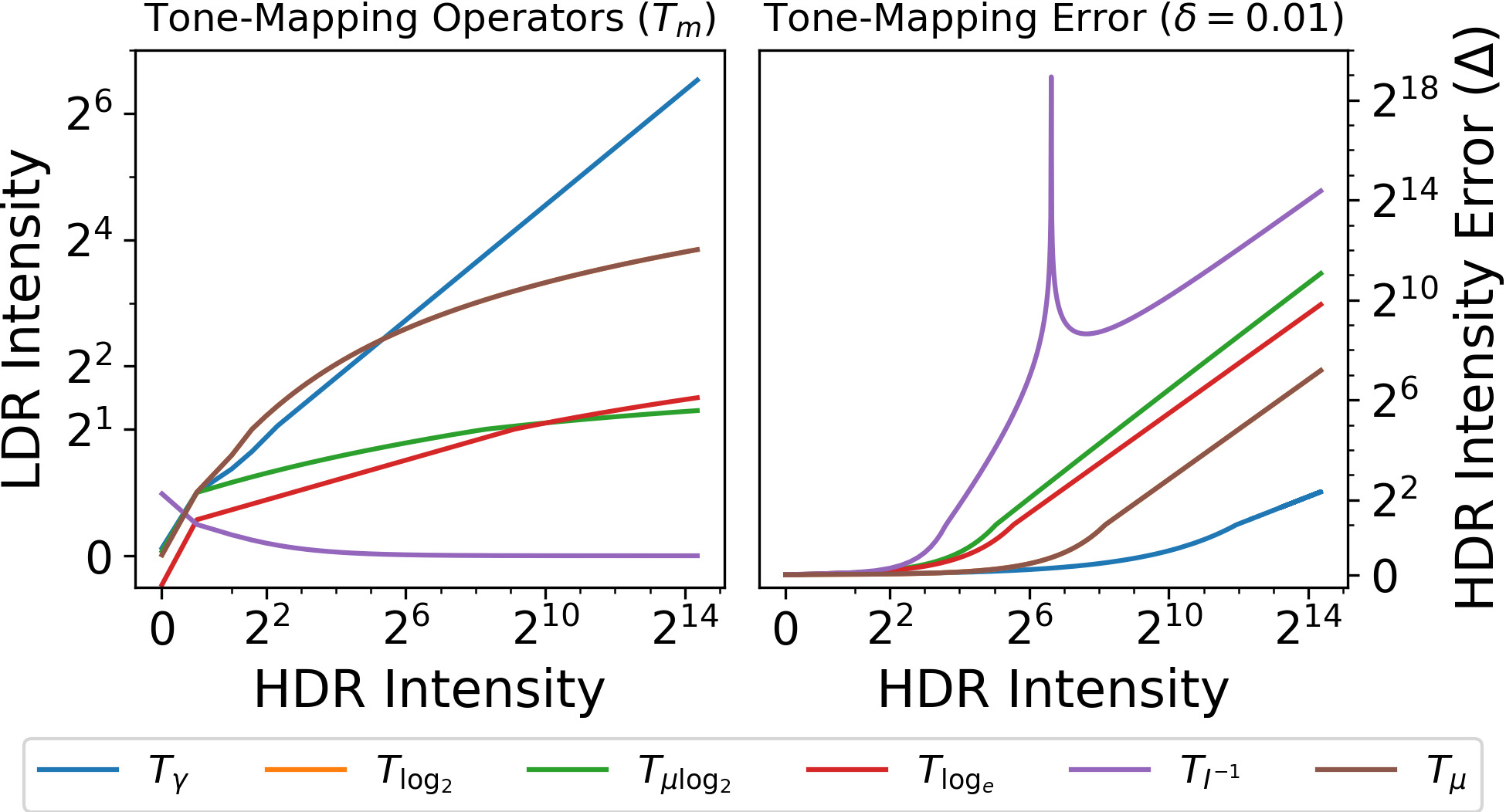
Each operator is a bijection allowing for the recovery of the original image via $\hat{I}={T_{m}}^{-1}(\check{I})$. Given $\Delta\hat{I}=|\hat{I}-{T_{m}}^{-1}({T_{m}}(\hat{I})-\delta)|$ as shown in Fig. 23 (right), these operators introduce a non-linearity between error ($\delta$) in LDR compressed space and error ($\Delta$) in uncompressed HDR space. The impact of non-linear-error is most pronounced with the solar disk (intensity-‘spike’ illustrated in Fig. 24), where a small error ($\delta$) to an LDR space solar disk results in a large error ($\Delta$) to the HDR space solar disk. This results in a profound impact to illumination in downstream applications such as IBL rendering.

B.2 Mitigation Strategies (Continued)

Strategies have been proposed to mitigate inaccurate modelling of solar luminous intensity including substitution of the solar disk [55], manual parametric boosting [10] and composite shading. In Figs. 25, 28, 27 and 26, we compare these mitigation strategies to AllSky [38] and Icarus ($512^{2}$ with RGB-styles and $f_{\text{\tiny Robertson}}$ fusion), implementing parametric Hošek-Wilkie clear skies (uniform 0.5 RGBalbedo, 1.0 turbidity) and suns [24, 25, 55], and boosting with a static set of user-selected parameters ($\gamma$=0.5, $\beta$=2, $\rho$=6) selected for similar solar intensity to FDR ground truth in Fig. 26. To mitigate calibration errors which might result in the misalignment of the solar disk, HW clear skies are matched FDR ground truth imagery (as done by CloudNet [55], though skipping histogram equalization).

As demonstrated in Figs. 25, 28, 27 and 26, mitigation strategy performance is varied, with no strategy generalizing to the four primary sky configurations: clear, cloudy, cloudy with overcast sun and overcast skies. As such, mitigation strategies require per-instance human intervention to make corrections and/or tune parameters. That said, AllSky and Icarus demonstrate reliable generalization across the four primaries, with renderings illustrating a high fidelity to ground truth illumination, shadows, tones and light transmission. Though some stochasticity in illumination is to be anticipated per natural real-world stochasticity in illumination, Icarus is shown to provide improved illumination accuracy and greater photorealism.

Figure 25: Overcast sky: Mitigation of solar modelling in environment maps through substitution of a parametric Hošek-Wilkie sun (HW [25, 55]) and manual parametric boosting of the HDR environment map (Boosted [10]; $\gamma$=0.5, $\beta$=2, $\rho$=6). Adding an HW sun (LDR+HW Sun) skips atmospheric attenuation and allows the sun to ‘pierce’ through clouds to create strong shadows. If the sun is obstructed, Boosting an HDR image (Boosted LDR) is prone to over-exposing and producing unpredictable shadows. Both mitigation strategies alter the perceived tones in IBL renderings (lambertian planar surface and color chart), but AllSky [38] and our model (Icarus, right column) accurately model real-world FDR illumination for photorealistic IBL renderings.

Figure 26: Cloudy with unobstructed sun: Mitigation of solar modelling in environment maps through substitution of a parametric Hošek-Wilkie sun (HW [25, 55]) and manual parametric boosting of the HDR environment map (Boosted [10]; $\gamma$=0.5, $\beta$=2, $\rho$=6). When the sun is unobstructed, adding an HW sun creates crisp shadows, realistic light-transmission (black glass orb) and only minor alteration of perceived tones (lambertian surface, color chart). Boosting an HDR image is subjective to user-selection of parameters, which drives both the algorithms’ selection of features and enhancement of intensity. Boosting is prone to over-exposing rendered scenes, producing unpredictable shadows, excessive light-transmission (black glass orb), and severe alteration of perceived tones (lambertian planar surface and color chart). While AllSky [38] mitigates the skewed tones from the parametric sun and over-saturation of boosting, Icarus (right column) offers greater photorealism and accuracy in illumination (EV and $\oiint_{I}$).

Figure 27: Cloudy with obstructed sun: Mitigation of solar modelling in environment maps through substitution of a parametric Hošek-Wilkie sun (HW [25, 55]) and manual parametric boosting of the HDR environment map (Boosted [10]; $\gamma$=0.5, $\beta$=2, $\rho$=6). Adding an HW sun skips atmospheric attenuation and allows the sun to ‘pierce’ through clouds to create strong shadows and unexpected light-transmission (black glass orb). If the sun is obstructed, boosting is prone to over-exposing (see skydome in $2^{nd}$ row and light-transmission to black-glass orb), producing unpredictable shadows and excessive light-transmission (black glass orb). AllSky [38] and Icarus both mitigate alteration of perceived tones (lambertian planar surface and color chart), with Icarus (right column) offering greater photorealism and accuracy in illumination (EV and $\oiint_{I}$).

Figure 28: Clear sky: Mitigation of solar modelling in environment maps through substitution of a parametric Hošek-Wilkie sun (HW [25, 55]) and manual parametric boosting of the HDR environment map (Boosted [10]; $\gamma$=0.5, $\beta$=2, $\rho$=6). In low-light settings such as dusk/sunset/sunrise, adding a parametric sun can be difficult given minor errors in camera calibration. Though an added HW sun ‘pierces’ through clouds formations with $10.9\!\times$ linear intensity of ground truth FDR Clear Sky, the absence of clouds acting as light-sources allows for relatively-indirect HW solar illumination to produce visually appealing renders without skewed tones. Boosting is subjective to user-selection of parameters driving the algorithms’ selection of features, which in low-light settings is shown to be prone to over-exposing the entirety of the skydome. This over-exposure results in unpredictable shadows (lambertian orb), excessive light-transmission (black glass orb) and altered tones (lambertian planar surface and color chart). AllSky [38] and Icarus both mitigate alteration of perceived tones (lambertian planar surface and color chart), producing renderings with accurate tones, shadows and light transmission.

Figure 29: Downsampling latlong environment maps from sky-angular shape $512^{2}$ to $64^{2}$. [Top row] Downsampling with area-interpolation retains illuminance ($\oiint_{I}$), but results in a loss of intensity from 14$EV$ to 11$EV$ (38% retention of linear space intensity). Though this has minimal impact to the visual quality of environment maps ($2^{nd}$ row), this is reflected in IBL scenes ($3^{rd}$ row, black glass orb) through a solar disk with increasing diameter both in the sky (not shown) and on incident surfaces (zoom box). As shown in the histograms (bottom row) of the zoom boxes, the intensity of light reflected off of the transmissible surface decrease from $2^{6.1}$ at $512^{2}$ to $2^{3.6}$ at $64^{2}$ (16% retention of linear space intensity).

B.3 Impact of Downsampling

As shown in Fig. 29, inter-area downsampling preserves an environment map’s luminance flux ($\oiint_{I}$), but dilation of the solar disk results in the loss of the exposure range ($EV$). The distinction between these measures is the quantification of global-illumination and peak-solar intensity, where in this example the four-pixels solar region with intensity $EV{\geq}11$ of the $512^{2}$ skydome represents 55% of the environment maps’ illumination. Though illuminance of the scene is consistent, the luminous intensity of the solar disk drives shadows and light-transmission, key to downstream applications including photorealistic IBL rendering [38] and simulating the output of solar systems [43].

Figure 30: Visual representation an LDR exposure bracket normalized to HDR-space by Eq. 3 for various tone mapping operators. Each LDR exposure is a ‘candle-stick’ where upper- and lower-limits illustrate min/max HDR intensities for $\check{I}$ clipped to $[0,1]$ and the body min/max HDR intensities for $\check{I}$ clipped to $[\epsilon,1-\epsilon]$ for $\epsilon=\underline{\epsilon}=\overline{\epsilon}=\frac{1}{255}$. Markers ($\circ$) indicate the HDR illumination intensity of an LDR exposure value of 0.5. Insufficient overlap and/or gaps between LDR exposures should be avoided during exposure selection.

Figure 31: Decomposition of an FDR image to LDR exposures by modulation of exposure $\Delta t=2^{-x}$, demonstrating atmospheric features are often visually indiscernible in exposures modulated by $2^{-6}$ or less. In exposure $2^{-14}$, the features of the solar corona is indiscernible and only the solar disk remains.

Appendix C Methodology (Extended)

We mathematically express images $I$ with the following modifiers and characteristics:

1. $I$: for an image

2. $\mathcal{I}$: for a generated image

3. $\check{I}$: for LDR colour images

4. $\hat{I}$: for HDR colour images

5. $\xi$: for latent images

6. $I_{c}$: for an image’s $c^{th}$ colour channel

7. $I_{ij}$: for row $i$ and col $j$ indexing of 2D matrices.

8. $I_{n,c,ij}$: for the $n^{th}$ exposure at color-channel $c$, row $i$ and col $j$ for 4D matrices of size $N\!\times\!C\!\times\!I\!\times\!J$.

9. $I_{n}$: for the $n^{th}$ image of an $N$-exposure LDR bracket.

10. $\{I_{n}\}^{N}$: for an $N$-exposures bracket (set) of $I_{n}$ images.

11. $k$: class $k$ of the set of classes $\mathcal{K}$

12. ${\mathchoice{\raisebox{0.0pt}{$\displaystyle\chi$}}{\raisebox{0.0pt}{$\textstyle\chi$}}{\raisebox{0.0pt}{$\scriptstyle\chi$}}{\raisebox{0.0pt}{$\scriptscriptstyle\chi$}}}_{k}$: for a style code for class $k$.

13. ${{\mathchoice{\raisebox{0.0pt}{$\displaystyle\chi$}}{\raisebox{0.0pt}{$\textstyle\chi$}}{\raisebox{0.0pt}{$\scriptstyle\chi$}}{\raisebox{0.0pt}{$\scriptscriptstyle\chi$}}}_{k}}^{\mathcal{K}}$: for the set of style codes corresponding to the $k$ classes in $\mathcal{K}$.

This allows for HDR images to be expressed as $\hat{I}_{n,c,ij}$ and LDR images part of an LDR bracket as $\{\check{I}_{n,c,ij}\}^{N}$. Where possible, we omit indiscriminative indexes to keep equations succinct.

C.1 LDR Bracketing

In Fig. 30 we expand the visual of LDR exposure brackets in Sec. 3.1 to include various tone mapping operators. By comparing candle-stick lower-limits and bodies, it can be shown that tone mapping operators can reduce the number of exposures required for coverage of a desired exposure range. This is well exemplified through the range of illumination intensity saturated in $T_{\varnothing}$’s lower limit but encompassed by $T_{\gamma}$’s elongated body. In this regard, Fig. 23 demonstrates the non-linearity of tone mapping operators where, for example, $T_{\gamma}$ decompresses values $<1$ and compresses values $>1$.

Careful consideration should be taken in determining requirements for overlapping exposures given tone mapping operator selection, distribution of image values, and desired granularity in modeling of HDR intensity. As illustrated in Fig. 31, linear coverage of FDR outdoor illumination intensity can result in many exposures with limited features and a limited ability to contribute to the desired exposure range.

C.2 LDR Exposure Fusion: HSV

We propose a simple fusion algorithm which takes advantage of HSVcolor space, converting $I_{{\color[rgb]{1,0,0}\definecolor[named]{pgfstrokecolor}{rgb}{1,0,0}R}{\color[rgb]{0,.5,.5}\definecolor[named]{pgfstrokecolor}{rgb}{0,.5,.5}G}{\color[rgb]{0,0,1}\definecolor[named]{pgfstrokecolor}{rgb}{0,0,1}B}}$ to $I_{{\color[rgb]{0,1,1}\definecolor[named]{pgfstrokecolor}{rgb}{0,1,1}\pgfsys@color@cmyk@stroke{1}{0}{0}{0}\pgfsys@color@cmyk@fill{1}{0}{0}{0}H}{\color[rgb]{1,0,0}\definecolor[named]{pgfstrokecolor}{rgb}{1,0,0}S}{\color[rgb]{.25,.25,.25}\definecolor[named]{pgfstrokecolor}{rgb}{.25,.25,.25}\pgfsys@color@gray@stroke{.25}\pgfsys@color@gray@fill{.25}V}}$ per [7]:

$${\color[rgb]{.25,.25,.25}\definecolor[named]{pgfstrokecolor}{rgb}{.25,.25,.25}\pgfsys@color@gray@stroke{.25}\pgfsys@color@gray@fill{.25}V}= \max({\color[rgb]{1,0,0}\definecolor[named]{pgfstrokecolor}{rgb}{1,0,0}R},{\color[rgb]{0,.5,.5}\definecolor[named]{pgfstrokecolor}{rgb}{0,.5,.5}G},{\color[rgb]{0,0,1}\definecolor[named]{pgfstrokecolor}{rgb}{0,0,1}B})$$ (22)

$${\color[rgb]{1,0,0}\definecolor[named]{pgfstrokecolor}{rgb}{1,0,0}S}= \begin{dcases}\frac{({\color[rgb]{.25,.25,.25}\definecolor[named]{pgfstrokecolor}{rgb}{.25,.25,.25}\pgfsys@color@gray@stroke{.25}\pgfsys@color@gray@fill{.25}V}-\min({\color[rgb]{1,0,0}\definecolor[named]{pgfstrokecolor}{rgb}{1,0,0}R},{\color[rgb]{0,.5,.5}\definecolor[named]{pgfstrokecolor}{rgb}{0,.5,.5}G},{\color[rgb]{0,0,1}\definecolor[named]{pgfstrokecolor}{rgb}{0,0,1}B})}{{\color[rgb]{.25,.25,.25}\definecolor[named]{pgfstrokecolor}{rgb}{.25,.25,.25}\pgfsys@color@gray@stroke{.25}\pgfsys@color@gray@fill{.25}V}}&\text{if }{\color[rgb]{.25,.25,.25}\definecolor[named]{pgfstrokecolor}{rgb}{.25,.25,.25}\pgfsys@color@gray@stroke{.25}\pgfsys@color@gray@fill{.25}V}\!\neq\!0\\ 0&\text{otherwise}\end{dcases}$$ (23)

$${\color[rgb]{0,1,1}\definecolor[named]{pgfstrokecolor}{rgb}{0,1,1}\pgfsys@color@cmyk@stroke{1}{0}{0}{0}\pgfsys@color@cmyk@fill{1}{0}{0}{0}H}= \begin{dcases}\frac{60({\color[rgb]{0,.5,.5}\definecolor[named]{pgfstrokecolor}{rgb}{0,.5,.5}G}-{\color[rgb]{0,0,1}\definecolor[named]{pgfstrokecolor}{rgb}{0,0,1}B})}{{\color[rgb]{.25,.25,.25}\definecolor[named]{pgfstrokecolor}{rgb}{.25,.25,.25}\pgfsys@color@gray@stroke{.25}\pgfsys@color@gray@fill{.25}V}-\min({\color[rgb]{1,0,0}\definecolor[named]{pgfstrokecolor}{rgb}{1,0,0}R},{\color[rgb]{0,.5,.5}\definecolor[named]{pgfstrokecolor}{rgb}{0,.5,.5}G},{\color[rgb]{0,0,1}\definecolor[named]{pgfstrokecolor}{rgb}{0,0,1}B})}&\text{if }{\color[rgb]{.25,.25,.25}\definecolor[named]{pgfstrokecolor}{rgb}{.25,.25,.25}\pgfsys@color@gray@stroke{.25}\pgfsys@color@gray@fill{.25}V}\!=\!{\color[rgb]{1,0,0}\definecolor[named]{pgfstrokecolor}{rgb}{1,0,0}R}\\ \frac{120+60({\color[rgb]{0,0,1}\definecolor[named]{pgfstrokecolor}{rgb}{0,0,1}B}-{\color[rgb]{1,0,0}\definecolor[named]{pgfstrokecolor}{rgb}{1,0,0}R})}{({\color[rgb]{.25,.25,.25}\definecolor[named]{pgfstrokecolor}{rgb}{.25,.25,.25}\pgfsys@color@gray@stroke{.25}\pgfsys@color@gray@fill{.25}V}-\min({\color[rgb]{1,0,0}\definecolor[named]{pgfstrokecolor}{rgb}{1,0,0}R},{\color[rgb]{0,.5,.5}\definecolor[named]{pgfstrokecolor}{rgb}{0,.5,.5}G},{\color[rgb]{0,0,1}\definecolor[named]{pgfstrokecolor}{rgb}{0,0,1}B}))}&\text{if }{\color[rgb]{.25,.25,.25}\definecolor[named]{pgfstrokecolor}{rgb}{.25,.25,.25}\pgfsys@color@gray@stroke{.25}\pgfsys@color@gray@fill{.25}V}\!=\!{\color[rgb]{0,.5,.5}\definecolor[named]{pgfstrokecolor}{rgb}{0,.5,.5}G}\\ \frac{240+60({\color[rgb]{1,0,0}\definecolor[named]{pgfstrokecolor}{rgb}{1,0,0}R}-{\color[rgb]{0,.5,.5}\definecolor[named]{pgfstrokecolor}{rgb}{0,.5,.5}G})}{({\color[rgb]{.25,.25,.25}\definecolor[named]{pgfstrokecolor}{rgb}{.25,.25,.25}\pgfsys@color@gray@stroke{.25}\pgfsys@color@gray@fill{.25}V}-\min({\color[rgb]{1,0,0}\definecolor[named]{pgfstrokecolor}{rgb}{1,0,0}R},{\color[rgb]{0,.5,.5}\definecolor[named]{pgfstrokecolor}{rgb}{0,.5,.5}G},{\color[rgb]{0,0,1}\definecolor[named]{pgfstrokecolor}{rgb}{0,0,1}B}))}&\text{if }{\color[rgb]{.25,.25,.25}\definecolor[named]{pgfstrokecolor}{rgb}{.25,.25,.25}\pgfsys@color@gray@stroke{.25}\pgfsys@color@gray@fill{.25}V}\!=\!{\color[rgb]{0,0,1}\definecolor[named]{pgfstrokecolor}{rgb}{0,0,1}B}\\ 0&\text{if }{\color[rgb]{1,0,0}\definecolor[named]{pgfstrokecolor}{rgb}{1,0,0}R}\!=\!{\color[rgb]{0,.5,.5}\definecolor[named]{pgfstrokecolor}{rgb}{0,.5,.5}G}\!=\!{\color[rgb]{0,0,1}\definecolor[named]{pgfstrokecolor}{rgb}{0,0,1}B}\end{dcases}$$ (24)

Converting images to HSVdisentangles brightness from chroma and hue, enabling the fusion of brightness channels (e.g. per Eq. 7 with $\check{I}_{c=V}$), and the creation of a fused HDR image by recombining as $\hat{I}_{{\color[rgb]{0,1,1}\definecolor[named]{pgfstrokecolor}{rgb}{0,1,1}\pgfsys@color@cmyk@stroke{1}{0}{0}{0}\pgfsys@color@cmyk@fill{1}{0}{0}{0}H}{\color[rgb]{1,0,0}\definecolor[named]{pgfstrokecolor}{rgb}{1,0,0}S}{\color[rgb]{.25,.25,.25}\definecolor[named]{pgfstrokecolor}{rgb}{.25,.25,.25}\pgfsys@color@gray@stroke{.25}\pgfsys@color@gray@fill{.25}V}}=\left\{\check{I}_{0,c={{\color[rgb]{0,1,1}\definecolor[named]{pgfstrokecolor}{rgb}{0,1,1}\pgfsys@color@cmyk@stroke{1}{0}{0}{0}\pgfsys@color@cmyk@fill{1}{0}{0}{0}H}}},\check{I}_{0,{c={\color[rgb]{1,0,0}\definecolor[named]{pgfstrokecolor}{rgb}{1,0,0}S}}},\hat{I}_{c={\color[rgb]{.25,.25,.25}\definecolor[named]{pgfstrokecolor}{rgb}{.25,.25,.25}\pgfsys@color@gray@stroke{.25}\pgfsys@color@gray@fill{.25}V}}\right\}$.

C.3 LDR Exposure Fusion: Robertson

Initial results showed that Robertson exposure fusion [53] lost visual performance due to conventional implementations (e.g. OpenCV [7]) requiring integer representation to support Look-Up-Table (LUT) weighting. As shown in Fig. 32(a) erroneous pixels appear within the solar corona and throughout the histogram in Fig. 32(c).

(a) Robertson (OpenCV [7])

(b) Robertson (Ours)

(c) Robertson (OpenCV [7])

(d) Robertson (Ours)

Figure 32: LDR exposure bracket $[2^{0},2^{8},2^{15}]$ merged with Robertson exposure fusion, as computed by OpenCV LUT [7] and by our inline implementation Eq. 26. As shown in Fig. 32(b), our implementation mitigates seams for a smoother FDR sun. Error between the ground truth (original, red outline) and reconstructed (rebuild, green outline) exposure range is shown in Fig. 32(c) and Fig. 32(d) to be significantly reduced.

We found discretization could be mitigated by re-implement the algorithm as an inline function:

$$W_{n} =\alpha e^{\frac{\psi\check{I}_{n}}{\lambda}-2}+\beta$$ (25)

$$\begin{split}\hat{I}&=f_{\text{\tiny Robertson}}\left(\left\{\check{I}_{n},\Delta{t}_{n}\right\}^{N}\right)\\ &=\sum_{n=1}^{N}\psi\Delta{t}_{n}W_{n}{\check{I}_{n}}\Bigg/\sum_{n=1}^{N}{\Delta{t}_{n}^{2}}W_{n}\end{split}$$ (26)

Where exposure $\check{I}_{n}$ is range $[0,1]$, LDR max value is $\psi\!=\!255$, scale is $\alpha\!=\!\frac{e^{4}}{e^{4}-1}$, shift is $\beta=\frac{1}{1-e^{4}}$, and $\lambda\!=\!(\psi_{LDR})/4\!=\!255/4$. As shown in Fig. 33, our inline function reproduces the Gaussian-like weighting and in Fig. 32(b) is shown to produce a smoother solar corona. The histogram in Fig. 32(c) also shows a significant reduction of error in image reconstruction.

Figure 33: Robertson weights by LDR index values ranged [0,255], as computed by OpenCV LUT [7] and by our inline implementation through Eq. 26. As shown, the weighting matches exactly.

We note Robertson include a priori assuming a Gaussian-like weighting of pixel values. This assumes the characteristics of conventional cameras but may be ill-suited to the noise characteristics of DNN-generated imagery.

Appendix D HDRDB Dataset

Figure 34: Example of ghosting in HDRDB [27], resulting in visual artifacts including discoloration and blurred cloud formations.

(a) Mean Skydome

(b) Mean Augmentation

(c) Overlayed segmentation

(d) Label

Figure 35: HDRDB mean and mean-augmented skydomes [27]. Labels (Fig. 35(d)) are 1-channel composites of solar, cloud, skydome (clear-sky), and border masks as proposed by [38]. Cloud segmentation is produced via colour ratio [13] and eroded to ‘hand-drawn’ representations Figure 35(d) is colourized for visualization purposes.

The Laval HDR Sky database (HDRDB, [27]) consists of 34K+ HDR images captured in Quebec City, Canada at varied intervals between 2014 and 2016 using a capture method synonymous to that proposed by Stumpfel et al. [61].

D.1 Known Flaws

For the purpose of this work, we ignore the presence of ‘ghosting’ in the dataset. As illustrated by the example in Fig. 34, ghosting is the result of the movement during the capture process which translates to visual artifacts in the recovered FDR imagery. Without knowledge of wind speed, altitude and other specifics, ghosting is an untractable characteristic of the dataset.

As we do not remove such flawed environment maps, we note that untractable artifacts including ‘ghosting’ impact measures of DNN model performance, prohibiting perfect reconstruction and modeling of all ‘features’ of the ground truth dataset. For the purpose of adversarial training, we assume discriminators learn to ignore the presence/absence of sporadic visual artifacts including ‘ghosting’. We justify this given sporadic artifacts are un-indicative of real or fake classification per a dataset with a fractional subset of HDRI with artifacts.

(a) Skydome (blue sky)

(b) Clouds

(c) Solar Corona

(d) Solar disk

Figure 36: Class-locality heat-maps for decomposed ‘hand-drawn’ HDRDB Discrete ($\mathbb{Z}^{+}$, Fig. 35(d)) labels. Heat-maps are colored from low- to high-frequency (red to blue), illustrating a disproportional volume of samples from summer months (high-solar elevation) and a near-constant ‘ring’ of clouds around the horizon.

Additionally, we note the distribution of samples in HDRDB is flawed temporally and geologically. As illustrated in Figs. 36(c) and 36(d), the bulk of HDRDB’s samples were captured during the summer months and favour sunset (west). As illustrated in Figs. 36(a) and 36(b), HDRDB’s samples are shown to exhibit a ‘crown of clouds’. When compared to wind and pressure maps, this appears to be the result of topology and pressure systems guiding cloud formations around Quebec City.

D.2 Environment Maps

For the purpose of this work, we assume that HDRDB latlong physically captured FDR HDRI were correctly captured, calibrated to linear RGB colour space with BT.709 primaries and converted to latlong format without loss. We assume no artifacts were introduced and no alterations were made to the exposure range or illumination.

D.3 Pre- and Post-Processing

To prevent discontinuities in generated skydomes, we convert the HDRI from latlong to sky-angular format as defined in Fig. 38. We reproduce the segmentation proposed by AllSky [38], expanding on previously identified challenges with environment map format conversions.

As illustrated in Fig. 37, loss of exposure range (EV) and illumination ($\oiint_{I}$) in downsampling HDRDB Sky-Latlong imagery is exacerbated by conversion to Sky-Angular format. In experimentation, we observed the findings to be exacerbated further if downsampling and format conversion are completed as a singular uniform transformation. To mitigate this destabilization of HDRI illumination characteristics, we convert formats at $\geq 2\times$ the target format resolution (inter-area upsampling if required), before inter-area downsampling (average pooling) to the target resolution. This approach (ours) is illustrated in Fig. 37 and shown to offer reliable downsampling.

Figure 37: Loss of exposure range (EV) and illumination ($\oiint_{I}$) in environment map format conversion and downsampling across 100 augmentations of an HDRI from June 7th, 2016 at 12:52PM [27]. Figs. 37 and 37 Left columns: Downsampling sky-latlong (sLL) environment maps. Figs. 37 and 37 Right columns: Converting and downsampling sky-latlong (sLL) environment maps to sky-angular (SA) format. The results show format conversions negatively impact exposure range and illumination, with Fig. 37 demonstrating the instability of output characteristics. Though spline (spline, order 1) interpolation preserves exposure ranges well in Fig. 37, Fig. 37 demonstrates significant variance in performance. Pooling (Pooled) can provide greater stability in downsampling (lower variance), where ours refers Icarus’s implementation of avg pooling while assuring format conversions are performed at $2\!\times$ target downsampling resolution. Adaptive average pooling (adp-avg) extends to offers support for downsampling arbitrarily (non powers of 2), which Icarus mitigates. Max pooling (max) results in steadily increasing environment luminance ($\oiint_{I}$).

D.4 Minimum Viable Resolution

From an extraterrestrial Point-Of-View (POV), the sun is a $0.5^{\circ}$ angular-diameter disk with near-constant illumination [56]. To accurately model the illumination and shadows cast by the solar disc, environment maps must offer pixel-granularity equal or greater to the angular size of the solar disk.

$$\Omega=2\pi\left(1-\cos\left({\frac{\theta}{2}}\right)\right)$$ (27)

The Field-Of-View (FOV) of an environment map’s pixel is expressed as solid angles in steradians ($\Omega$). Using Eq. 27 with the solar disk angular diameter in radians ($\theta$), the solar disk represents $5.98\times 10^{-5}$ steradians. Comparing to the maximum solid angle of common environment map formats, this translates to a minimum resolution of $512^{2}$ in sky-angular format. This translates to resolution of $1024\!\times\!2048$ in latlong (equirectangular) format.

D.5 Subsets and Augmentation

Figure 38: Sky-Angular Environment Map

From the database—the mean of which is shown in Fig. 35(a)—we augment the dataset with random rotations around the zenith to increase solar placement coverage (Fig. 35(b)) and enable generation of skies outside of HDRDB. We split the dataset into training (23,249), validation (2,576), and testing (6,634) subsets by arbitrarily splitting by date of capture such that each subset has a random assortment of images from each year and season of capture. We then prune these subsets to remove images where solar elevation is less than $10^{\circ}$ as the sun is obfuscated (apparent sunset) and the resulting low-light is reflected by poor image quality. This reduces the aforementioned training (20,064), validation (2,238), and testing (5,811) subset sizes. For ablation studies, the training subset is further reduced to 4,096 samples while retaining the full validation and testing subsets.

Note, among other, we do not account for the distribution of solar elevations, solar intensities, cloud coverage, wind speeds, or families of cloud formations across subsets. As shown in Figs. 36(c) and 36(d), the bulk of HDRDB’s samples were captured during the summer months and favour sunset (west). As a results, sunrise, sunset, winter and other settings are underrepresented.

D.6 Segmentation

We recreate the segmentation of HDRDB proposed by AllSky [38] to create ‘hand-drawn’ labels of the environment maps.

Solar positioning is refined from ephemeris calculations [60], labelling the extraterrestrial 0.5^∘ sun as the solar disk. To reflect terrestrial imagery, we extend the masked solar-region to a diameter of $5^{\circ}$ to include the solar corona and atmospheric attenuation of the extraterrestrial solar disc.

Cloud formations are segmented by thresholding the ratio $Y=\frac{B-R}{B+R}$ proposed by Dev et al. [13] to $\mu$LawLog₂ tone mapped HDRI. Clouds masks are further processed morphologically to reduce complexity and produce ‘hand-drawn’ masks emulating having been drawn with circular brush (kernel size 15). The final label is a 1-channel composite of solar, cloud, skydome (clear-sky), and border masks as shown in Fig. 35(d).

The accuracy of this approach is illustrated by the overlayed label in Fig. 35(c). Note, segmentation exhibits variability with illumination intensity (e.g. sunrise/sunset) and seasonality [33].

D.7 Tone Mapping Operators

For visualization of the impact on LDR-space intensity by tone mapping operators, we include the mean histograms from tone mapping HDRDB (all subsets, 34K+ HDR images) with $T_{\gamma}$ and $T_{\mu\log_{2}}$ tone mapping operators in Figs. 39 and 40.

Figure 39: Histogram of Power-Law ($T_{\gamma}$) tone-mapped HDRDB [27]

Figure 40: Histogram of $\mu$-lawLog₂ ($T_{\mu\log_{2}}$) tone-mapped HDRDB [27]

D.8 Metrics

Recent works have shown HDR imagery should be evaluated as perceptually uniform (PU) values such that quantization is aligned to human perception of visible differences [36]. We do not implement a perceptually uniform encoding function as HDRDB: 1. Is not metrically calibrated for luminance 2. The original physically captured LDR brackets are not available 3. Records of the platform’s CRF, intrinsic, colorimetric, photometric and most other calibration are unavailable/lost.

Figure 41: SEAN [71]

Appendix E Models

In the following subsections, we expand on our baselines and model variants.

E.1 SEAN

We selected SEAN [71] as a proven model for image-translation and configured as shown in Fig. 41 to train a baseline. Although initial experimentation was successful, we found a significant number of errors in the authors’ code base, including:

1. The dimension of the latent z-vector is set by default to $z\_dim=256$ in configuration but is fused to $z\_dim=512$ at (style encoder) initialization.

2. Adversarial training is non-functional due to a cut gradient in the hinge-loss.Footnote 7

3. The adversarial Feature Matching Loss does not positively contribute to results .

We found that fixing the adversarial hinge loss destabilized training, resulting in frequent collapses . We therefore discarded SEAN’s discriminator and replaced it with one of our own design, integrating the Adversarial Feature Matching Loss [66].

E.2 SEAN (Ours)

We create our own implementation of SEAN by refactoring all modules for improved throughput and footprint. This reduced SEAN’s parameters by 25% (from 266 to 200 million parameters at a resolution of $512^{2}$) and significantly improves computational performance.

We redesigned the static generator architecture to be dynamically configurable, allowing for a desired input seed-label shape (e.g. $32^{2}$) or a desired number of upsampling layers. This change is necessary to accommodate HDRDB semantic labels where key classes (e.g. the solar disk) can be lost in seed-label shapes below $32^{2}$.

E.3 Icarus (Ours)

We adopt SEAN (Ours) as a backbone architecture and develop a decoder supporting the generation of FDR exposure ranges as LDR exposure brackets. We characterize the final layer of the architecture as the decoder (‘latent $\rightarrow$ RGB’ in Fig. 41) and explore different decoder architectures (Icarus decoder in Fig. 5).

(a) SPADE: SPADE with $x$-features

(b) SPADE+: SPADE with $x$-features per exposures

(c) SPADE^N: One Spade per Exposure

Figure 42: Decoder architectures for LDR bracket generation, exploring configurations of SPADE (S) blocks and their output features. In Fig. 42(b), SPADE+ is configured such that SPADE outputs n-features per exposure as indicated by ${\Rrightarrow}$ instead of $\rightarrow$.

E.3.1 Decoder: SPADE

We implement a simple variant which replaces the output convolution layer (d) with n-parallel convolutional layers ($d_{0},d_{n},\dots,d_{N}$). As illustrated in Figs. 42(a) and 42(b), we explore SPADE (S,[71]) output features, passing them uniformly ($\rightarrow$; denoted as SPADE) and equally-split ($\Rrightarrow$, grouping by n-exposures; denoted as SPADE+) to n-parallel convolution layers.

E.3.2 Decoder: n-SPADE

As illustrated in Fig. 42(c), we explore a larger architecture which implemented n-SPADE blocks ($S_{0},S_{n},\dots,S_{N}$; denoted as SPADE³). This allowed for independent modulation of features for each exposure of a LDR exposure bracket.

E.3.3 Decoder: Additional Configuration Details

We found enabling affine synchronized batch normalization in the SPADE blocks of the decoder improved performance. We note that synchronous training of all decoders with decayed exposure facilitates training and provides better visual results. Due to the limited features shared between low and high exposures, exposure decay (see Sec. 3.2.2) aligns features and mitigates collapse. Asynchronous incremental training of the model is precarious as effort must be taken to ensure visual quality of $\check{I}_{0}$ is not lost/degraded in training higher exposures $\check{I}_{k>0}$. We note that a model trained to generate $\check{I}_{0}$ does not generalize well to $\check{I}_{k>0}$ and therefore recommend the generator (G) not be frozen during training of higher exposures.

E.3.4 RGB-Style Encoder Augmentation

We note that supervised losses are possible with SEAN as the model learns to reconstruct the input per segmentation and style-codes distilled from paired ground truth imagery. This entanglement between input and generated imagery is undesirable, but cannot be fully mitigated given the contents of environment maps are not necessarily translatable (e.g. an overcast sun presumably cannot be substituted for a clear-sky’s sun). To mitigate and discourage entanglement with ground truth imagery, we augment the input to the style-encoder with flips and rotations around the zenith. We further $T_{\gamma}$ tone-map and clip style-encoder input to LDR space.

E.3.5 RGB-Style Code Limitations

In training, style encoder inputs are independently augmented, but we do not address the reconstruction enabled from paired segmentation, style-codes, and ground truth imagery. This is particularly difficult, given the architecture is ignorant of lens calibration and thus does not distill the same style-code for the same texture sampled at the horizon and at the zenith. As such, not all styles are translatable from one segmentation to another (e.g. clouds at the horizon to clouds at the zenith).

To address this issue, a methodology for sampling textures as style codes independent of positioning would need to be developed. Addressing this issue was determined to be outside the scope of the contributions of this work, but is believed to be feasible through a study of style-codes. This would involve undistorting textures while ensuring a uniform granularity of sampled textures.

E.3.6 Independently Training The RND-Style Mapper

Our default training routine for Icarus is oriented around uniformly training of the generator per a singular source of style-codes. If Icarus’s generator is trained with the RGB-style encoder, it is possible for the RND-style mapper to learn RGB-style encoder’s distribution of codes. This can be achieved by iteratively decaying the weight of per-exposures losses per Eq. 6 for a simulated incremental training of exposures.

Additionally, we explored the mixing of RGB- and RND- styles during training. Though we do not report this work, we found that passing subsets of the RGB-style codes through the mapper can aid in training the mapper. This suggests a complementary training routine could be developed which uniformly trains Icarus with both the RGB-style encoder and RND- style mapper.

E.3.7 Independently Training The RGB-Style Encoder

We do not report training the RGB-style encoder per a frozen generator trained with the RND-style mapper, but the encoder and mapper are fully interchangeable.

E.4 Fusion

We decompose fusion with the objective of mitigating the priori of a Gaussian-like weighting of pixel values. We achieve this by proposing $f_{\text{\tiny DNN}}$ in Eq. 7 to predict content-aware weights for each exposure of an LDR bracket $\left\{\check{I}_{n}\right\}^{N}$.

As shown in Fig. 43, we experiment with two architectures which enable class-aware modulation of $\left\{\check{I}_{n}\right\}^{N}$ via a SPADE [71] per $\left\{\check{I}_{n}\right\}^{N}$ input or generator latent $\xi$ input. In Fig. 43(a), a weight $\left\{W_{n}\right\}^{N}$ is generated to be uniformly applied to LDR exposures $\left\{\check{I}_{n}\right\}^{N}$ and exposures times $\left\{\Delta t_{n}\right\}^{N}$ as shown in Eq. 29. In Fig. 43(b), separate weights $\left\{W^{\Delta t}_{n}\right\}^{N}$ and $\left\{W^{e}_{n}\right\}^{N}$ are generated for LDR exposures $\left\{\check{I}_{n}\right\}^{N}$ and exposures times $\left\{\Delta t_{n}\right\}^{N}$ as shown in Eq. 30. Additionally, we explore passing SPADE ($S$) features uniformly ($\rightarrow$) and equally-split ($\Rrightarrow$, grouped by exposure) to convolutional layers.

$$\hat{I} =f_{\text{\tiny DNN}}\left(\left\{\check{I}_{n},\Delta{t}_{n}\right\}^{N}\right)$$ (28)

$$=\sum_{n=1}^{N}\Delta{t}_{n}W_{n}{\check{I}_{n}}\Bigg/\sum_{n=1}^{N}{\Delta{t}_{n}^{2}}W_{n}$$ (29)

$$=\sum_{n=1}^{N}\Delta{t}_{n}W^{e}_{n}{\check{I}_{n}}\Bigg/\sum_{n=1}^{N}{\Delta{t}_{n}^{2}}W^{\Delta t}_{n}$$ (30)

(a) Uniform Weights $W^{e}_{n}=W^{\Delta t}_{n}=W_{n,c,ij}$.

(b) Separate weights $W^{e}_{n,c,ij}$ and $W^{\Delta t}_{n,c,ij}$.

Figure 43: Architectures for LDR bracket Fusion. In Fig. 43(a), a weight $W_{n,c,ij}$ is generated to be uniformly applied to LDR exposures $\left\{\check{I}_{n}\right\}^{N}$ and exposures times $\left\{\Delta t_{n}\right\}^{N}$. In Fig. 43(b), a separate weight $W^{e}_{n,c,ij}$ is generated to module exposures $\left\{\check{I}_{n}\right\}^{N}$ and a $W^{\Delta t}_{n,c,ij}$ to modulate exposures times $\left\{\Delta t_{n}\right\}^{N}$. Features output by SPADE (${\Rrightarrow}$) are configurable to output n-features or n-features per exposure.

Figure 44: Sensitivity of various commonly reported HDR metrics to truncation of the exposure range. As shown, Integrated Illumination ($\oiint_{I}$, Eq. 1), Peak-Luminance ($PL_{\Omega}$ Eq. 15, Peak Ill. Int.$I_{\Omega}$), and VIF [57] offer sensitivity to truncations of HDR-space exposure. Though PSNR offers sensitivity in LDR-space, the metric offers little sensitivity in HDR-space. HDR-VDP3 offers little sensitivity to truncations of exposure in both LDR- and HDR-space.

Table 2: The results show that training with the Discriminator Feature Matching loss (indicated by *) negatively impacts cLDR metrics with higher FID and MiFID scores. Though $\mu\text{-lawLog}_{2}$ ($T_{\mu\log_{2}}$) tone mapping generally offers better cLDR metric performance, FDR performance is variable and prone to over-exposure ($\oiint_{I}$). Gamma ($T_{\gamma}$) tone mapping offers similar cLDR performance with stable exposure range (EV) and illumination ($\oiint_{I}$). Average training time is reduced by over 50%, from 9hr 15min for SEAN to 4hr 25min for SEAN (Ours) with no loss in model performance. Bold values indicate category best and underlined values indicate overall best.

		System	$T_{\gamma}$-cLDR			HDR
	$T_{m}$	Time	LPIPS $\downarrow$	FID $\downarrow$	MiFID $\downarrow$	HDR-VDP3 $\uparrow$	PSNR${}_{\log_{2}}$ $\uparrow$	EV $\leftarrow$	$\oiint_{I}\leftarrow$
Ground Truth $128^{2}$	-	-	-	-	-	-	-	7.34	1.22
SEAN*	$T_{\gamma}$	8:31	0.16	19.6	303	8.29	140	6.94	1.04
SEAN*	$T_{\mu\log_{2}}$	8:22	0.16	21.6	322	7.96	115	7.27	3.38
SEAN	$T_{\gamma}$	9:28	0.16	20.0	306	8.25	138	7.16	1.08
SEAN	$T_{\mu\log_{2}}$	10:25	0.16	18.5	292	8.04	123	6.49	1.6$e^{6}$
SEAN* (Ours)	$T_{\gamma}$	5:06	0.15	27.9	385	8.48	140	7.15	1.16
SEAN* (Ours)	$T_{\mu\log_{2}}$	4:24	0.14	20.9	320	8.25	125	6.28	0.98
SEAN (Ours)	$T_{\gamma}$	4:17	0.15	17.6	275	8.46	138	7.03	1.16
SEAN (Ours)	$T_{\mu\log_{2}}$	3:56	0.15	16.8	269	8.08	124	5.93	0.93
Ground Truth $256^{2}$	-	-	-	-	-	-	-	8.58	1.22
SEAN* (Ours)	$T_{\gamma}$	-	0.18	22.3	348	8.28	159	8.81	1.12
SEAN* (Ours)	$T_{\mu\log_{2}}$	-	0.18	20.9	334	8.20	138	8.25	1.05
SEAN (Ours)	$T_{\gamma}$	-	0.18	19.9	322	8.28	159	8.44	1.02
SEAN (Ours)	$T_{\mu\log_{2}}$	-	0.18	19.0	308	8.00	127	8.97	3.34
Ground Truth $512^{2}$	-	-	-	-	-	-	-	9.62	1.22
SEAN* (Ours)	$T_{\gamma}$	-	0.21	53.8	662	7.32	152	7.84	0.72
SEAN* (Ours)	$T_{\mu\log_{2}}$	-	0.21	45.2	587	7.59	147	4.83	0.87
SEAN (Ours)	$T_{\gamma}$	-	0.36	186.4	-	4.43	-	24.86	$3e^{5}$
SEAN (Ours)	$T_{\mu\log_{2}}$	-	0.28	144.2	-	2.62	-	118.72	$1e^{32}$

Appendix F Experiments

In the following sections, we expand on our reported results to include more detailed discussion of our baselines and experimentation.

F.1 SEAN

We train SEAN [71] and SEAN (Ours) at a resolution of $128^{2}$ to demonstrate the equivalence of the models. As shown in Tab. 2, SEAN (Ours) achieves similar or better cLDR and FDR performance while reducing the computational expense by over 50%.

At low resolution, the results in Tab. 2 demonstrate that SEAN’s Discriminator-Feature Matching loss negatively impacts cLDR performance with higher FID and MiFID scores. As shown through lost performance as resolution is doubled from $128^{2}$ to $512^{2}$, SEAN (Ours) is negatively impacted by increasing exposure range. This coincides with findings by AllSKy [38] which identified that increasing resolution results in the solar region becoming the predominant means of differentiation at higher resolutions. Though quantitatively the Discriminator Feature Matching loss mitigates numerical overflow at a resolution of $512^{2}$, the quality of the generated images is undesirable. Given the negative impact to cLDR performance at low exposure ranges (implicit per low resolution) and poor FDR performance, we elected to omit SEAN’s Discriminator Feature Matching loss in later experimentation.

Handling of exposure range is crucial to the performance of DNN sky-models. Tone mapping provides a means of mitigating, but AllSky [38] found tone mapping introduces non-linearity between error in LDR and HDR space, resulting in unstable illumination. This finding is reflected in Tab. 2, with aggressive $\mu\text{-lawLog}_{2}$ ($T_{\mu\log_{2}}$) tone mapping offering better cLDR metric performance but variable FDR performance prone to over- and under-exposure ($\oiint_{I}$). As a result, we conclude weaker Gamma ($T_{\gamma}$) tone mapping fosters greater stability in model performance.

Table 3: We ablate Icarus to ascertain the impact of multiple exposures on visual quality by training for a singular exposure $[2^{0}]$ ($1\!\times\!f_{\text{\tiny{\color[rgb]{1,0,0}\definecolor[named]{pgfstrokecolor}{rgb}{1,0,0}R}{\color[rgb]{0,.5,.5}\definecolor[named]{pgfstrokecolor}{rgb}{0,.5,.5}G}{\color[rgb]{0,0,1}\definecolor[named]{pgfstrokecolor}{rgb}{0,0,1}B}}}$) and three exposures $[2^{0},2^{0},2^{0}]$ ($3\!\times\!f_{\text{\tiny{\color[rgb]{1,0,0}\definecolor[named]{pgfstrokecolor}{rgb}{1,0,0}R}{\color[rgb]{0,.5,.5}\definecolor[named]{pgfstrokecolor}{rgb}{0,.5,.5}G}{\color[rgb]{0,0,1}\definecolor[named]{pgfstrokecolor}{rgb}{0,0,1}B}}}$). As in Tab. 2, the results show that training with the Discriminator Feature Matching loss (indicated by *) negatively impacts cLDR metrics with higher FID and MiFID scores. Aggressive $\mu\text{-lawLog}_{2}$ ($T_{\mu\log_{2}}$) tone mapping offers better cLDR metric performance and is shown to retain a larger exposure range in FDR metrics. As denoted by ^†, exposures are clipped in LDR-space, crippling FDR performance. The results show that overlapping exposures negatively impact cLDR performance by introducing noise. This is reflected in lost performance in repeating model evaluation with RGB- ($3\!\times\!f_{\text{\tiny{\color[rgb]{1,0,0}\definecolor[named]{pgfstrokecolor}{rgb}{1,0,0}R}{\color[rgb]{0,.5,.5}\definecolor[named]{pgfstrokecolor}{rgb}{0,.5,.5}G}{\color[rgb]{0,0,1}\definecolor[named]{pgfstrokecolor}{rgb}{0,0,1}B}}}$) and HSV-fusion ($3\!\times\!f_{\text{\tiny{\color[rgb]{0,1,1}\definecolor[named]{pgfstrokecolor}{rgb}{0,1,1}\pgfsys@color@cmyk@stroke{1}{0}{0}{0}\pgfsys@color@cmyk@fill{1}{0}{0}{0}H}{\color[rgb]{1,0,0}\definecolor[named]{pgfstrokecolor}{rgb}{1,0,0}S}{\color[rgb]{.25,.25,.25}\definecolor[named]{pgfstrokecolor}{rgb}{.25,.25,.25}\pgfsys@color@gray@stroke{.25}\pgfsys@color@gray@fill{.25}V}}}$), where HSV-fusion sustains performance by retaining chroma only from the first exposure. Bold values indicate category best and underlined values indicate overall best.

		$T_{\gamma}$-cLDR			HDR
	$T_{m}$	LPIPS $\downarrow$	FID $\downarrow$	MiFID $\downarrow$	HDR-VDP3 $\uparrow$	†PSNR${}_{\log_{2}}$ $\uparrow$	†EV $\leftarrow$	†$\oiint_{I}\leftarrow$
Ground Truth $128^{2}$	-	-	-	-	-	-	7.34	1.22
Icarus* (SPADEn; $1\!\times\!f_{\text{\tiny{\color[rgb]{1,0,0}\definecolor[named]{pgfstrokecolor}{rgb}{1,0,0}R}{\color[rgb]{0,.5,.5}\definecolor[named]{pgfstrokecolor}{rgb}{0,.5,.5}G}{\color[rgb]{0,0,1}\definecolor[named]{pgfstrokecolor}{rgb}{0,0,1}B}}}$)	$T_{\gamma}$	0.14	16.0	255	7.7	124	1.57	0.60
Icarus* (SPADEn; $1\!\times\!f_{\text{\tiny{\color[rgb]{1,0,0}\definecolor[named]{pgfstrokecolor}{rgb}{1,0,0}R}{\color[rgb]{0,.5,.5}\definecolor[named]{pgfstrokecolor}{rgb}{0,.5,.5}G}{\color[rgb]{0,0,1}\definecolor[named]{pgfstrokecolor}{rgb}{0,0,1}B}}}$)	$T_{\mu\log_{2}}$	0.14	19.1	307	7.8	124	2.91	0.68
Icarus (SPADEn; $1\!\times\!f_{\text{\tiny{\color[rgb]{1,0,0}\definecolor[named]{pgfstrokecolor}{rgb}{1,0,0}R}{\color[rgb]{0,.5,.5}\definecolor[named]{pgfstrokecolor}{rgb}{0,.5,.5}G}{\color[rgb]{0,0,1}\definecolor[named]{pgfstrokecolor}{rgb}{0,0,1}B}}}$)	$T_{\gamma}$	0.14	19.0	306	7.8	122	1.72	0.77
Icarus (SPADEn; $1\!\times\!f_{\text{\tiny{\color[rgb]{1,0,0}\definecolor[named]{pgfstrokecolor}{rgb}{1,0,0}R}{\color[rgb]{0,.5,.5}\definecolor[named]{pgfstrokecolor}{rgb}{0,.5,.5}G}{\color[rgb]{0,0,1}\definecolor[named]{pgfstrokecolor}{rgb}{0,0,1}B}}}$)	$T_{\mu\log_{2}}$	0.14	15.7	260	7.9	124	3.30	0.69
Icarus* (SPADEn; $3\!\times\!f_{\text{\tiny{\color[rgb]{1,0,0}\definecolor[named]{pgfstrokecolor}{rgb}{1,0,0}R}{\color[rgb]{0,.5,.5}\definecolor[named]{pgfstrokecolor}{rgb}{0,.5,.5}G}{\color[rgb]{0,0,1}\definecolor[named]{pgfstrokecolor}{rgb}{0,0,1}B}}}$)	$T_{\gamma}$	0.15	24.1	377	7.7	123	$1.62$	$0.65$
Icarus* (SPADEn; $3\!\times\!f_{\text{\tiny{\color[rgb]{1,0,0}\definecolor[named]{pgfstrokecolor}{rgb}{1,0,0}R}{\color[rgb]{0,.5,.5}\definecolor[named]{pgfstrokecolor}{rgb}{0,.5,.5}G}{\color[rgb]{0,0,1}\definecolor[named]{pgfstrokecolor}{rgb}{0,0,1}B}}}$)	$T_{\mu\log_{2}}$	0.14	21.2	335	7.9	124	3.17	0.67
Icarus (SPADEn; $3\!\times\!f_{\text{\tiny{\color[rgb]{1,0,0}\definecolor[named]{pgfstrokecolor}{rgb}{1,0,0}R}{\color[rgb]{0,.5,.5}\definecolor[named]{pgfstrokecolor}{rgb}{0,.5,.5}G}{\color[rgb]{0,0,1}\definecolor[named]{pgfstrokecolor}{rgb}{0,0,1}B}}}$)	$T_{\gamma}$	0.14	25.2	383	7.8	123	$1.60$	0.63
Icarus (SPADEn; $3\!\times\!f_{\text{\tiny{\color[rgb]{1,0,0}\definecolor[named]{pgfstrokecolor}{rgb}{1,0,0}R}{\color[rgb]{0,.5,.5}\definecolor[named]{pgfstrokecolor}{rgb}{0,.5,.5}G}{\color[rgb]{0,0,1}\definecolor[named]{pgfstrokecolor}{rgb}{0,0,1}B}}}$)	$T_{\mu\log_{2}}$	0.14	21.8	350	7.8	124	$\mathbf{2.81}$	$0.62$
Icarus* (SPADEn; $3\!\times\!f_{\text{\tiny{\color[rgb]{0,1,1}\definecolor[named]{pgfstrokecolor}{rgb}{0,1,1}\pgfsys@color@cmyk@stroke{1}{0}{0}{0}\pgfsys@color@cmyk@fill{1}{0}{0}{0}H}{\color[rgb]{1,0,0}\definecolor[named]{pgfstrokecolor}{rgb}{1,0,0}S}{\color[rgb]{.25,.25,.25}\definecolor[named]{pgfstrokecolor}{rgb}{.25,.25,.25}\pgfsys@color@gray@stroke{.25}\pgfsys@color@gray@fill{.25}V}}}$)	$T_{\gamma}$	0.15	18.4	299	7.6	142	$1.64$	$0.65$
Icarus* (SPADEn; $3\!\times\!f_{\text{\tiny{\color[rgb]{0,1,1}\definecolor[named]{pgfstrokecolor}{rgb}{0,1,1}\pgfsys@color@cmyk@stroke{1}{0}{0}{0}\pgfsys@color@cmyk@fill{1}{0}{0}{0}H}{\color[rgb]{1,0,0}\definecolor[named]{pgfstrokecolor}{rgb}{1,0,0}S}{\color[rgb]{.25,.25,.25}\definecolor[named]{pgfstrokecolor}{rgb}{.25,.25,.25}\pgfsys@color@gray@stroke{.25}\pgfsys@color@gray@fill{.25}V}}}$)	$T_{\mu\log_{2}}$	0.14	15.7	262	7.8	142	$\mathbf{3.42}$	$\mathbf{0.67}$
Icarus (SPADEn; $3\!\times\!f_{\text{\tiny{\color[rgb]{0,1,1}\definecolor[named]{pgfstrokecolor}{rgb}{0,1,1}\pgfsys@color@cmyk@stroke{1}{0}{0}{0}\pgfsys@color@cmyk@fill{1}{0}{0}{0}H}{\color[rgb]{1,0,0}\definecolor[named]{pgfstrokecolor}{rgb}{1,0,0}S}{\color[rgb]{.25,.25,.25}\definecolor[named]{pgfstrokecolor}{rgb}{.25,.25,.25}\pgfsys@color@gray@stroke{.25}\pgfsys@color@gray@fill{.25}V}}}$)	$T_{\gamma}$	0.14	18.9	304	7.7	143	$1.6$	$0.61$
Icarus (SPADEn; $3\!\times\!f_{\text{\tiny{\color[rgb]{0,1,1}\definecolor[named]{pgfstrokecolor}{rgb}{0,1,1}\pgfsys@color@cmyk@stroke{1}{0}{0}{0}\pgfsys@color@cmyk@fill{1}{0}{0}{0}H}{\color[rgb]{1,0,0}\definecolor[named]{pgfstrokecolor}{rgb}{1,0,0}S}{\color[rgb]{.25,.25,.25}\definecolor[named]{pgfstrokecolor}{rgb}{.25,.25,.25}\pgfsys@color@gray@stroke{.25}\pgfsys@color@gray@fill{.25}V}}}$)	$T_{\mu\log_{2}}$	0.14	18.6	307	7.7	143	$\mathbf{2.99}$	$\mathbf{0.63}$

F.2 Icarus with RGB-Style Encoder

In Tab. 3, we ablate Icarus to ascertain the impact of generating multiple exposures. The results show that overlapping exposures introduce noise in fused HDR images which is reflected by a loss in cLDR metric performance. The impact of this noise is demonstrated through the gap between RGB- and HSV-fusion performance, where HSV-fusion sustains performance by retaining chroma only from the first exposure. As shown by comparison of SPADEⁿ variants in Tab. 4, this performance gap is mitigatable by limiting exposure overlap.

We expand on this ablation in Tabs. 4 and 5 to determine the impact of decoder architecture selection on cohesion between exposures and further study tone mapping. As show in Tab. 4, tone mapping improves cLDR and FDR performance, though some bias may exist given LPIPS’ conditioning on $T_{\gamma}$ LDR imagery. The results show SPADE+ decoder architecture with $T_{\gamma}$ tone mapping comparatively offers better performance and no cohesion between exposures is necessary at the convolution layer. This reflected through comparatively improved performance with SPADE+ block conditioning on all exposures in Tab. 4, and comparatively lower performance in Tab. 5 given cohesion between exposures at the convolution layer.

In table Tab. 6 we ablate our discriminators to ascertain their conditioning of Icarus with SPADE+, finding that training with both the LDR and HDR discriminators provides a performance advantage with larger exposure ranges. The evaluation of these models was repeated with various fusion operators, demonstrating Robertson fusion ($f_{\text{\tiny Robertson}}$) significantly improves visual quality, while RGB ($f_{\text{\tiny{\color[rgb]{1,0,0}\definecolor[named]{pgfstrokecolor}{rgb}{1,0,0}R}{\color[rgb]{0,.5,.5}\definecolor[named]{pgfstrokecolor}{rgb}{0,.5,.5}G}{\color[rgb]{0,0,1}\definecolor[named]{pgfstrokecolor}{rgb}{0,0,1}B}}}$) and HSV ($f_{\text{\tiny{\color[rgb]{0,1,1}\definecolor[named]{pgfstrokecolor}{rgb}{0,1,1}\pgfsys@color@cmyk@stroke{1}{0}{0}{0}\pgfsys@color@cmyk@fill{1}{0}{0}{0}H}{\color[rgb]{1,0,0}\definecolor[named]{pgfstrokecolor}{rgb}{1,0,0}S}{\color[rgb]{.25,.25,.25}\definecolor[named]{pgfstrokecolor}{rgb}{.25,.25,.25}\pgfsys@color@gray@stroke{.25}\pgfsys@color@gray@fill{.25}V}}}$) fusion offer improved illumination. Debevec fusion ($f_{\text{\tiny Debevec}}$) is shown to underperform across both visual quality and illumination metrics.

Table 4: We ablate Icarus with SPADE, SPADE+ and SPADEⁿ decoder architectures to ascertain the requirement for cohesion between SPADE features. We train Icarus with $T_{\gamma}$ and $T_{\mu\log_{2}}$ tone mapping for exposure set $[2^{0},2^{-8},2^{-12}]$ and train Icarus without tone mapping ($T_{\varnothing}$) for exposures $[2^{0},2^{-8},2^{-15}]$. Model evaluation is repeated for RGB- and HSV-fusion, demonstrating the absence of a gap between RGBand HSV-fusion performance which suggests limiting exposure overlap reduces noise in fused imagery. The results demonstrate that tone mapping ($T_{\gamma}$ or $T_{\mu\log_{2}}$) improves cLDR and FDR performance, with $T_{\varnothing}$ under-performing for all configurations. Bold values indicate category best and underlined values indicate overall best. In this regard, the SPADE+ decoder architecture with $T_{\gamma}$ tone mapping is shown to comparatively offer better cLDR and FDR performance.

		$T_{\gamma}$-cLDR			HDR
	$T_{m}$	LPIPS $\downarrow$	FID $\downarrow$	MiFID $\downarrow$	HDR-VDP3 $\uparrow$	PSNR${}_{\log_{2}}$ $\uparrow$	EV $\leftarrow$	$\oiint_{I}\leftarrow$
Ground Truth $128^{2}$	-	-	-	-	-	-	7.96	1.22
Icarus (SPADEn; $f_{\text{\tiny{\color[rgb]{1,0,0}\definecolor[named]{pgfstrokecolor}{rgb}{1,0,0}R}{\color[rgb]{0,.5,.5}\definecolor[named]{pgfstrokecolor}{rgb}{0,.5,.5}G}{\color[rgb]{0,0,1}\definecolor[named]{pgfstrokecolor}{rgb}{0,0,1}B}}}$)	$T_{\gamma}$	0.14	19.8	316	8.4	147	7.37	0.92
Icarus (SPADE+; $f_{\text{\tiny{\color[rgb]{1,0,0}\definecolor[named]{pgfstrokecolor}{rgb}{1,0,0}R}{\color[rgb]{0,.5,.5}\definecolor[named]{pgfstrokecolor}{rgb}{0,.5,.5}G}{\color[rgb]{0,0,1}\definecolor[named]{pgfstrokecolor}{rgb}{0,0,1}B}}}$)	$T_{\gamma}$	0.14	18.8	306	8.5	147	8.03	1.05
Icarus (SPADE; $f_{\text{\tiny{\color[rgb]{1,0,0}\definecolor[named]{pgfstrokecolor}{rgb}{1,0,0}R}{\color[rgb]{0,.5,.5}\definecolor[named]{pgfstrokecolor}{rgb}{0,.5,.5}G}{\color[rgb]{0,0,1}\definecolor[named]{pgfstrokecolor}{rgb}{0,0,1}B}}}$)	$T_{\gamma}$	0.15	23.8	351	8.4	139	8.60	1.25
Icarus (SPADEn; $f_{\text{\tiny{\color[rgb]{1,0,0}\definecolor[named]{pgfstrokecolor}{rgb}{1,0,0}R}{\color[rgb]{0,.5,.5}\definecolor[named]{pgfstrokecolor}{rgb}{0,.5,.5}G}{\color[rgb]{0,0,1}\definecolor[named]{pgfstrokecolor}{rgb}{0,0,1}B}}}$)	$T_{\mu\log_{2}}$	0.15	22.0	328	8.4	145	7.75	1.05
Icarus (SPADE+; $f_{\text{\tiny{\color[rgb]{1,0,0}\definecolor[named]{pgfstrokecolor}{rgb}{1,0,0}R}{\color[rgb]{0,.5,.5}\definecolor[named]{pgfstrokecolor}{rgb}{0,.5,.5}G}{\color[rgb]{0,0,1}\definecolor[named]{pgfstrokecolor}{rgb}{0,0,1}B}}}$)	$T_{\mu\log_{2}}$	0.14	23.9	354	8.5	147	7.82	1.01
Icarus (SPADE; $f_{\text{\tiny{\color[rgb]{1,0,0}\definecolor[named]{pgfstrokecolor}{rgb}{1,0,0}R}{\color[rgb]{0,.5,.5}\definecolor[named]{pgfstrokecolor}{rgb}{0,.5,.5}G}{\color[rgb]{0,0,1}\definecolor[named]{pgfstrokecolor}{rgb}{0,0,1}B}}}$)	$T_{\mu\log_{2}}$	0.14	22.3	340	8.4	147	7.92	1.07
Icarus (SPADEn; $f_{\text{\tiny{\color[rgb]{1,0,0}\definecolor[named]{pgfstrokecolor}{rgb}{1,0,0}R}{\color[rgb]{0,.5,.5}\definecolor[named]{pgfstrokecolor}{rgb}{0,.5,.5}G}{\color[rgb]{0,0,1}\definecolor[named]{pgfstrokecolor}{rgb}{0,0,1}B}}}$)	$T_{\varnothing}$	0.20	71.2	790	7.8	138	7.73	0.96
Icarus (SPADE+; $f_{\text{\tiny{\color[rgb]{1,0,0}\definecolor[named]{pgfstrokecolor}{rgb}{1,0,0}R}{\color[rgb]{0,.5,.5}\definecolor[named]{pgfstrokecolor}{rgb}{0,.5,.5}G}{\color[rgb]{0,0,1}\definecolor[named]{pgfstrokecolor}{rgb}{0,0,1}B}}}$)	$T_{\varnothing}$	0.17	35.1	462	7.0	116	9.54	3.74
Icarus (SPADE; $f_{\text{\tiny{\color[rgb]{1,0,0}\definecolor[named]{pgfstrokecolor}{rgb}{1,0,0}R}{\color[rgb]{0,.5,.5}\definecolor[named]{pgfstrokecolor}{rgb}{0,.5,.5}G}{\color[rgb]{0,0,1}\definecolor[named]{pgfstrokecolor}{rgb}{0,0,1}B}}}$)	$T_{\varnothing}$	0.16	37.4	496	8.1	127	8.91	1.54
Icarus (SPADEn; $f_{\text{\tiny{\color[rgb]{0,1,1}\definecolor[named]{pgfstrokecolor}{rgb}{0,1,1}\pgfsys@color@cmyk@stroke{1}{0}{0}{0}\pgfsys@color@cmyk@fill{1}{0}{0}{0}H}{\color[rgb]{1,0,0}\definecolor[named]{pgfstrokecolor}{rgb}{1,0,0}S}{\color[rgb]{.25,.25,.25}\definecolor[named]{pgfstrokecolor}{rgb}{.25,.25,.25}\pgfsys@color@gray@stroke{.25}\pgfsys@color@gray@fill{.25}V}}}$)	$T_{\gamma}$	0.14	21.3	345	8.3	147	7.38	0.95
Icarus (SPADE+; $f_{\text{\tiny{\color[rgb]{0,1,1}\definecolor[named]{pgfstrokecolor}{rgb}{0,1,1}\pgfsys@color@cmyk@stroke{1}{0}{0}{0}\pgfsys@color@cmyk@fill{1}{0}{0}{0}H}{\color[rgb]{1,0,0}\definecolor[named]{pgfstrokecolor}{rgb}{1,0,0}S}{\color[rgb]{.25,.25,.25}\definecolor[named]{pgfstrokecolor}{rgb}{.25,.25,.25}\pgfsys@color@gray@stroke{.25}\pgfsys@color@gray@fill{.25}V}}}$)	$T_{\gamma}$	0.14	18.9	312	8.5	147	7.95	1.06
Icarus (SPADE; $f_{\text{\tiny{\color[rgb]{0,1,1}\definecolor[named]{pgfstrokecolor}{rgb}{0,1,1}\pgfsys@color@cmyk@stroke{1}{0}{0}{0}\pgfsys@color@cmyk@fill{1}{0}{0}{0}H}{\color[rgb]{1,0,0}\definecolor[named]{pgfstrokecolor}{rgb}{1,0,0}S}{\color[rgb]{.25,.25,.25}\definecolor[named]{pgfstrokecolor}{rgb}{.25,.25,.25}\pgfsys@color@gray@stroke{.25}\pgfsys@color@gray@fill{.25}V}}}$)	$T_{\gamma}$	0.15	22.3	355	8.4	140	8.52	1.27
Icarus (SPADEn; $f_{\text{\tiny{\color[rgb]{0,1,1}\definecolor[named]{pgfstrokecolor}{rgb}{0,1,1}\pgfsys@color@cmyk@stroke{1}{0}{0}{0}\pgfsys@color@cmyk@fill{1}{0}{0}{0}H}{\color[rgb]{1,0,0}\definecolor[named]{pgfstrokecolor}{rgb}{1,0,0}S}{\color[rgb]{.25,.25,.25}\definecolor[named]{pgfstrokecolor}{rgb}{.25,.25,.25}\pgfsys@color@gray@stroke{.25}\pgfsys@color@gray@fill{.25}V}}}$)	$T_{\mu\log_{2}}$	0.15	19.1	306	8.3	146	7.61	1.05
Icarus (SPADE+; $f_{\text{\tiny{\color[rgb]{0,1,1}\definecolor[named]{pgfstrokecolor}{rgb}{0,1,1}\pgfsys@color@cmyk@stroke{1}{0}{0}{0}\pgfsys@color@cmyk@fill{1}{0}{0}{0}H}{\color[rgb]{1,0,0}\definecolor[named]{pgfstrokecolor}{rgb}{1,0,0}S}{\color[rgb]{.25,.25,.25}\definecolor[named]{pgfstrokecolor}{rgb}{.25,.25,.25}\pgfsys@color@gray@stroke{.25}\pgfsys@color@gray@fill{.25}V}}}$)	$T_{\mu\log_{2}}$	0.14	21.9	345	8.4	147	7.76	1.02
Icarus (SPADE; $f_{\text{\tiny{\color[rgb]{0,1,1}\definecolor[named]{pgfstrokecolor}{rgb}{0,1,1}\pgfsys@color@cmyk@stroke{1}{0}{0}{0}\pgfsys@color@cmyk@fill{1}{0}{0}{0}H}{\color[rgb]{1,0,0}\definecolor[named]{pgfstrokecolor}{rgb}{1,0,0}S}{\color[rgb]{.25,.25,.25}\definecolor[named]{pgfstrokecolor}{rgb}{.25,.25,.25}\pgfsys@color@gray@stroke{.25}\pgfsys@color@gray@fill{.25}V}}}$)	$T_{\mu\log_{2}}$	0.14	24.4	381	8.3	148	7.65	1.04
Icarus (SPADEn; $f_{\text{\tiny{\color[rgb]{0,1,1}\definecolor[named]{pgfstrokecolor}{rgb}{0,1,1}\pgfsys@color@cmyk@stroke{1}{0}{0}{0}\pgfsys@color@cmyk@fill{1}{0}{0}{0}H}{\color[rgb]{1,0,0}\definecolor[named]{pgfstrokecolor}{rgb}{1,0,0}S}{\color[rgb]{.25,.25,.25}\definecolor[named]{pgfstrokecolor}{rgb}{.25,.25,.25}\pgfsys@color@gray@stroke{.25}\pgfsys@color@gray@fill{.25}V}}}$)	$T_{\varnothing}$	0.20	70.2	872	7.8	140	8.01	1.08
Icarus (SPADE+; $f_{\text{\tiny{\color[rgb]{0,1,1}\definecolor[named]{pgfstrokecolor}{rgb}{0,1,1}\pgfsys@color@cmyk@stroke{1}{0}{0}{0}\pgfsys@color@cmyk@fill{1}{0}{0}{0}H}{\color[rgb]{1,0,0}\definecolor[named]{pgfstrokecolor}{rgb}{1,0,0}S}{\color[rgb]{.25,.25,.25}\definecolor[named]{pgfstrokecolor}{rgb}{.25,.25,.25}\pgfsys@color@gray@stroke{.25}\pgfsys@color@gray@fill{.25}V}}}$)	$T_{\varnothing}$	0.17	25.0	380	6.7	110	9.44	4.19
Icarus (SPADE; $f_{\text{\tiny{\color[rgb]{0,1,1}\definecolor[named]{pgfstrokecolor}{rgb}{0,1,1}\pgfsys@color@cmyk@stroke{1}{0}{0}{0}\pgfsys@color@cmyk@fill{1}{0}{0}{0}H}{\color[rgb]{1,0,0}\definecolor[named]{pgfstrokecolor}{rgb}{1,0,0}S}{\color[rgb]{.25,.25,.25}\definecolor[named]{pgfstrokecolor}{rgb}{.25,.25,.25}\pgfsys@color@gray@stroke{.25}\pgfsys@color@gray@fill{.25}V}}}$)	$T_{\varnothing}$	0.15	33.4	491	7.6	127	9.09	2.01

Table 5: We ablate Icarus decoder architectures with a singular output convolution layer (denoted by $\dagger$) instead of parallelized per-exposure output convolution layers as done in Tab. 4. Icarus is trained for SPADE, SPADE+ and SPADEⁿ architecture and exposures $[2^{0},2^{-8},2^{-12}]$ with $T_{\gamma}$ and $T_{\mu\log_{2}}$ tone mapping. Model evaluation is repeated for RGB- and HSV-fusion, with Bold values indicating category best and underlined values indicating overall best. The results demonstrate that $T_{\gamma}$ tone mapping improves SPADE performance, while $T_{\mu\log_{2}}$ tone mapping improves SPADE+ performance. The SPADE and SPADE+ decoder architecture differ only in the number of generated latent features (n-features vs. n-features-per-exposure) and offer similar performance improvement in comparison to SPADEⁿ. Given overall cLDR and FDR metrics, SPADE offers better performance over SPADE+, demonstrating increasing latent features does not correlate to improved visual quality. In comparison to Tab. 4, the results demonstrate that parallelized per-exposure output convolution layers offer improved performance.

		$T_{\gamma}$-cLDR			HDR
	$T_{m}$	LPIPS $\downarrow$	FID $\downarrow$	MiFID $\downarrow$	HDR-VDP3 $\uparrow$	PSNR${}_{\log_{2}}$ $\uparrow$	EV $\leftarrow$	$\oiint_{I}\leftarrow$
Ground Truth $128^{2}$	-	-	-	-	-	-	7.96	1.22
Icarus (SPADEn; $f_{\text{\tiny{\color[rgb]{1,0,0}\definecolor[named]{pgfstrokecolor}{rgb}{1,0,0}R}{\color[rgb]{0,.5,.5}\definecolor[named]{pgfstrokecolor}{rgb}{0,.5,.5}G}{\color[rgb]{0,0,1}\definecolor[named]{pgfstrokecolor}{rgb}{0,0,1}B}}}$)†	$T_{\gamma}$	0.14	25.5	368	8.5	149	7.88	1.07
Icarus (SPADE+; $f_{\text{\tiny{\color[rgb]{1,0,0}\definecolor[named]{pgfstrokecolor}{rgb}{1,0,0}R}{\color[rgb]{0,.5,.5}\definecolor[named]{pgfstrokecolor}{rgb}{0,.5,.5}G}{\color[rgb]{0,0,1}\definecolor[named]{pgfstrokecolor}{rgb}{0,0,1}B}}}$)†	$T_{\gamma}$	0.15	22.6	343	8.5	148	7.93	1.16
Icarus (SPADE; $f_{\text{\tiny{\color[rgb]{1,0,0}\definecolor[named]{pgfstrokecolor}{rgb}{1,0,0}R}{\color[rgb]{0,.5,.5}\definecolor[named]{pgfstrokecolor}{rgb}{0,.5,.5}G}{\color[rgb]{0,0,1}\definecolor[named]{pgfstrokecolor}{rgb}{0,0,1}B}}}$)†	$T_{\gamma}$	0.14	19.5	311	8.5	149	7.93	1.09
Icarus (SPADEn; $f_{\text{\tiny{\color[rgb]{1,0,0}\definecolor[named]{pgfstrokecolor}{rgb}{1,0,0}R}{\color[rgb]{0,.5,.5}\definecolor[named]{pgfstrokecolor}{rgb}{0,.5,.5}G}{\color[rgb]{0,0,1}\definecolor[named]{pgfstrokecolor}{rgb}{0,0,1}B}}}$)†	$T_{\mu\log_{2}}$	0.15	25.3	384	8.5	150	7.58	1.00
Icarus (SPADE+; $f_{\text{\tiny{\color[rgb]{1,0,0}\definecolor[named]{pgfstrokecolor}{rgb}{1,0,0}R}{\color[rgb]{0,.5,.5}\definecolor[named]{pgfstrokecolor}{rgb}{0,.5,.5}G}{\color[rgb]{0,0,1}\definecolor[named]{pgfstrokecolor}{rgb}{0,0,1}B}}}$)†	$T_{\mu\log_{2}}$	0.14	20.1	317	8.4	148	7.52	1.03
Icarus (SPADE; $f_{\text{\tiny{\color[rgb]{1,0,0}\definecolor[named]{pgfstrokecolor}{rgb}{1,0,0}R}{\color[rgb]{0,.5,.5}\definecolor[named]{pgfstrokecolor}{rgb}{0,.5,.5}G}{\color[rgb]{0,0,1}\definecolor[named]{pgfstrokecolor}{rgb}{0,0,1}B}}}$)†	$T_{\mu\log_{2}}$	0.15	22.2	330	8.3	149	7.23	0.89
Icarus (SPADEn; $f_{\text{\tiny{\color[rgb]{0,1,1}\definecolor[named]{pgfstrokecolor}{rgb}{0,1,1}\pgfsys@color@cmyk@stroke{1}{0}{0}{0}\pgfsys@color@cmyk@fill{1}{0}{0}{0}H}{\color[rgb]{1,0,0}\definecolor[named]{pgfstrokecolor}{rgb}{1,0,0}S}{\color[rgb]{.25,.25,.25}\definecolor[named]{pgfstrokecolor}{rgb}{.25,.25,.25}\pgfsys@color@gray@stroke{.25}\pgfsys@color@gray@fill{.25}V}}}$)†	$T_{\gamma}$	0.14	21.7	345	8.5	148	7.87	1.07
Icarus (SPADE+; $f_{\text{\tiny{\color[rgb]{0,1,1}\definecolor[named]{pgfstrokecolor}{rgb}{0,1,1}\pgfsys@color@cmyk@stroke{1}{0}{0}{0}\pgfsys@color@cmyk@fill{1}{0}{0}{0}H}{\color[rgb]{1,0,0}\definecolor[named]{pgfstrokecolor}{rgb}{1,0,0}S}{\color[rgb]{.25,.25,.25}\definecolor[named]{pgfstrokecolor}{rgb}{.25,.25,.25}\pgfsys@color@gray@stroke{.25}\pgfsys@color@gray@fill{.25}V}}}$)†	$T_{\gamma}$	0.15	21.7	345	8.4	147	7.92	1.17
Icarus (SPADE; $f_{\text{\tiny{\color[rgb]{0,1,1}\definecolor[named]{pgfstrokecolor}{rgb}{0,1,1}\pgfsys@color@cmyk@stroke{1}{0}{0}{0}\pgfsys@color@cmyk@fill{1}{0}{0}{0}H}{\color[rgb]{1,0,0}\definecolor[named]{pgfstrokecolor}{rgb}{1,0,0}S}{\color[rgb]{.25,.25,.25}\definecolor[named]{pgfstrokecolor}{rgb}{.25,.25,.25}\pgfsys@color@gray@stroke{.25}\pgfsys@color@gray@fill{.25}V}}}$)†	$T_{\gamma}$	0.14	20.9	342	8.4	148	8.03	1.14
Icarus (SPADEn; $f_{\text{\tiny{\color[rgb]{0,1,1}\definecolor[named]{pgfstrokecolor}{rgb}{0,1,1}\pgfsys@color@cmyk@stroke{1}{0}{0}{0}\pgfsys@color@cmyk@fill{1}{0}{0}{0}H}{\color[rgb]{1,0,0}\definecolor[named]{pgfstrokecolor}{rgb}{1,0,0}S}{\color[rgb]{.25,.25,.25}\definecolor[named]{pgfstrokecolor}{rgb}{.25,.25,.25}\pgfsys@color@gray@stroke{.25}\pgfsys@color@gray@fill{.25}V}}}$)†	$T_{\mu\log_{2}}$	0.15	25.4	400	8.4	149	7.64	1.02
Icarus (SPADE+; $f_{\text{\tiny{\color[rgb]{0,1,1}\definecolor[named]{pgfstrokecolor}{rgb}{0,1,1}\pgfsys@color@cmyk@stroke{1}{0}{0}{0}\pgfsys@color@cmyk@fill{1}{0}{0}{0}H}{\color[rgb]{1,0,0}\definecolor[named]{pgfstrokecolor}{rgb}{1,0,0}S}{\color[rgb]{.25,.25,.25}\definecolor[named]{pgfstrokecolor}{rgb}{.25,.25,.25}\pgfsys@color@gray@stroke{.25}\pgfsys@color@gray@fill{.25}V}}}$)†	$T_{\mu\log_{2}}$	0.14	19.7	326	8.3	147	7.55	1.04
Icarus (SPADE; $f_{\text{\tiny{\color[rgb]{0,1,1}\definecolor[named]{pgfstrokecolor}{rgb}{0,1,1}\pgfsys@color@cmyk@stroke{1}{0}{0}{0}\pgfsys@color@cmyk@fill{1}{0}{0}{0}H}{\color[rgb]{1,0,0}\definecolor[named]{pgfstrokecolor}{rgb}{1,0,0}S}{\color[rgb]{.25,.25,.25}\definecolor[named]{pgfstrokecolor}{rgb}{.25,.25,.25}\pgfsys@color@gray@stroke{.25}\pgfsys@color@gray@fill{.25}V}}}$)†	$T_{\mu\log_{2}}$	0.15	20.7	331	8.2	149	7.26	0.90

Table 6: We ablate our adversarial LDR and HDR discriminators to ascertain their conditioning of Icarus with SPADE+ for exposures $[2^{0},2^{-8},2^{-14}]$ and $T_{\gamma}$ tone mapping. Evaluation is repeated for RGB-, HSV-, Robertson- (ours) and Debevec-fusion [11]. Bold values indicate category best and underlined values indicate overall best. Fusion operators offer contrasting performance, with Roberson-fusion significantly improving visual quality (cLDR) metrics and RGB- and HSV-fusion offer improved illumination (FDR metrics). As shown, Debevec-fusion underperforms in terms of both visual quality and illumination metrics. At a resolution of $128^{2}$, our HDR discriminator outperforms our LDR discriminator, and no advantage is gained from training with both (LDR+HDR) discriminators. When resolution is doubled to $256^{2}$, training with both (LDR+HDR) discriminators provides a clear advantage, offering better handling of the (linear) doubling of the exposure range.

		$T_{\gamma}$-cLDR			HDR
	$T_{m}$	LPIPS $\downarrow$	FID $\downarrow$	MiFID $\downarrow$	HDR-VDP3 $\uparrow$	PSNR${}_{\log_{2}}$ $\uparrow$	EV $\leftarrow$	$\oiint_{I}\leftarrow$
Ground Truth $128^{2}$	-	-	-	-	-	-	7.96	1.22
Icarus (LDR; $f_{\text{\tiny{\color[rgb]{1,0,0}\definecolor[named]{pgfstrokecolor}{rgb}{1,0,0}R}{\color[rgb]{0,.5,.5}\definecolor[named]{pgfstrokecolor}{rgb}{0,.5,.5}G}{\color[rgb]{0,0,1}\definecolor[named]{pgfstrokecolor}{rgb}{0,0,1}B}}}$)	$T_{\gamma}$	0.14	26.0	388	8.54	149	7.91	1.06
Icarus (HDR; $f_{\text{\tiny{\color[rgb]{1,0,0}\definecolor[named]{pgfstrokecolor}{rgb}{1,0,0}R}{\color[rgb]{0,.5,.5}\definecolor[named]{pgfstrokecolor}{rgb}{0,.5,.5}G}{\color[rgb]{0,0,1}\definecolor[named]{pgfstrokecolor}{rgb}{0,0,1}B}}}$)	$T_{\gamma}$	0.14	23.9	357	8.57	150	7.79	1.08
Icarus (LDR+HDR; $f_{\text{\tiny{\color[rgb]{1,0,0}\definecolor[named]{pgfstrokecolor}{rgb}{1,0,0}R}{\color[rgb]{0,.5,.5}\definecolor[named]{pgfstrokecolor}{rgb}{0,.5,.5}G}{\color[rgb]{0,0,1}\definecolor[named]{pgfstrokecolor}{rgb}{0,0,1}B}}}$)	$T_{\gamma}$	0.14	23.9	362	8.46	147	7.85	0.98
Icarus (LDR; $f_{\text{\tiny{\color[rgb]{0,1,1}\definecolor[named]{pgfstrokecolor}{rgb}{0,1,1}\pgfsys@color@cmyk@stroke{1}{0}{0}{0}\pgfsys@color@cmyk@fill{1}{0}{0}{0}H}{\color[rgb]{1,0,0}\definecolor[named]{pgfstrokecolor}{rgb}{1,0,0}S}{\color[rgb]{.25,.25,.25}\definecolor[named]{pgfstrokecolor}{rgb}{.25,.25,.25}\pgfsys@color@gray@stroke{.25}\pgfsys@color@gray@fill{.25}V}}}$)	$T_{\gamma}$	0.14	24.6	390	8.54	149	7.98	1.10
Icarus (HDR; $f_{\text{\tiny{\color[rgb]{0,1,1}\definecolor[named]{pgfstrokecolor}{rgb}{0,1,1}\pgfsys@color@cmyk@stroke{1}{0}{0}{0}\pgfsys@color@cmyk@fill{1}{0}{0}{0}H}{\color[rgb]{1,0,0}\definecolor[named]{pgfstrokecolor}{rgb}{1,0,0}S}{\color[rgb]{.25,.25,.25}\definecolor[named]{pgfstrokecolor}{rgb}{.25,.25,.25}\pgfsys@color@gray@stroke{.25}\pgfsys@color@gray@fill{.25}V}}}$)	$T_{\gamma}$	0.14	20.5	333	8.54	150	7.76	1.10
Icarus (LDR+HDR; $f_{\text{\tiny{\color[rgb]{0,1,1}\definecolor[named]{pgfstrokecolor}{rgb}{0,1,1}\pgfsys@color@cmyk@stroke{1}{0}{0}{0}\pgfsys@color@cmyk@fill{1}{0}{0}{0}H}{\color[rgb]{1,0,0}\definecolor[named]{pgfstrokecolor}{rgb}{1,0,0}S}{\color[rgb]{.25,.25,.25}\definecolor[named]{pgfstrokecolor}{rgb}{.25,.25,.25}\pgfsys@color@gray@stroke{.25}\pgfsys@color@gray@fill{.25}V}}}$)	$T_{\gamma}$	0.14	25.6	405	8.38	148	7.82	0.95
Icarus (LDR; $f_{\text{\tiny Robertson}}$)	$T_{\gamma}$	0.13	16.3	269	7.41	146	7.82	1.05
Icarus (HDR; $f_{\text{\tiny Robertson}}$)	$T_{\gamma}$	0.13	15.0	250	6.42	144	7.63	1.04
Icarus (LDR+HDR; $f_{\text{\tiny Robertson}}$)	$T_{\gamma}$	0.13	16.9	284	7.77	148	7.64	0.97
Icarus (LDR; $f_{\text{\tiny Debevec}}$)	$T_{\gamma}$	0.26	51.0	554	3.44	116	8.37	1.66
Icarus (HDR; $f_{\text{\tiny Debevec}}$)	$T_{\gamma}$	0.26	53.4	584	3.44	115	8.54	1.70
Icarus (LDR+HDR; $f_{\text{\tiny Debevec}}$)	$T_{\gamma}$	0.26	55.7	625	3.43	116	8.39	1.60
Ground Truth $256^{2}$	-	-	-	-	-	-	9.36	1.22
Icarus (LDR; $f_{\text{\tiny{\color[rgb]{1,0,0}\definecolor[named]{pgfstrokecolor}{rgb}{1,0,0}R}{\color[rgb]{0,.5,.5}\definecolor[named]{pgfstrokecolor}{rgb}{0,.5,.5}G}{\color[rgb]{0,0,1}\definecolor[named]{pgfstrokecolor}{rgb}{0,0,1}B}}}$)	$T_{\gamma}$	0.17	34.9	512	8.30	168	9.54	1.05
Icarus (HDR; $f_{\text{\tiny{\color[rgb]{1,0,0}\definecolor[named]{pgfstrokecolor}{rgb}{1,0,0}R}{\color[rgb]{0,.5,.5}\definecolor[named]{pgfstrokecolor}{rgb}{0,.5,.5}G}{\color[rgb]{0,0,1}\definecolor[named]{pgfstrokecolor}{rgb}{0,0,1}B}}}$)	$T_{\gamma}$	0.17	33.2	490	8.27	168	9.46	1.11
Icarus (LDR+HDR; $f_{\text{\tiny{\color[rgb]{1,0,0}\definecolor[named]{pgfstrokecolor}{rgb}{1,0,0}R}{\color[rgb]{0,.5,.5}\definecolor[named]{pgfstrokecolor}{rgb}{0,.5,.5}G}{\color[rgb]{0,0,1}\definecolor[named]{pgfstrokecolor}{rgb}{0,0,1}B}}}$)	$T_{\gamma}$	0.18	31.5	465	8.33	170	9.59	1.08
Icarus (LDR; 3xHSV)	$T_{\gamma}$	0.17	38.6	606	8.24	168	9.7	1.1
Icarus (HDR; 3xHSV)	$T_{\gamma}$	0.17	34.9	537	8.23	168	9.51	1.17
Icarus (LDR+HDR; 3xHSV)	$T_{\gamma}$	0.18	32.9	516	8.31	170	9.75	1.13
Icarus (LDR; $f_{\text{\tiny Robertson}}$)	$T_{\gamma}$	0.17	22.5	372	8.20	169	9.51	1.06
Icarus (HDR; $f_{\text{\tiny Robertson}}$)	$T_{\gamma}$	0.17	23.0	375	8.20	168	9.44	1.10
Icarus (LDR+HDR; $f_{\text{\tiny Robertson}}$)	$T_{\gamma}$	0.17	20.5	338	8.21	171	9.49	1.08
Icarus (LDR; $f_{\text{\tiny Debevec}}$)	$T_{\gamma}$	-	-	-	-	-	-	-
Icarus (HDR; $f_{\text{\tiny Debevec}}$)	$T_{\gamma}$	0.26	62.0	690	3.27	137	9.67	1.49
Icarus (LDR+HDR; $f_{\text{\tiny Debevec}}$)	$T_{\gamma}$	-	-	-	-	-	-	-

F.3 Icarus with RND-Style Mapper

In Tab. 7 we evaluate Icarus trained exclusively with our RND-style mapper. This faster variant is trained is trained with the same subsets of HDRDB defined in Sec. D.5 and the same parameters, but requires prolonged training to first establish the RND-style mapper. As such, this variant is trained for 400 epochs with all exposure decoder heads set to $\Delta t_{0}=1$, then uniformly decayed to target exposures over 400 epochs.

Please note, we could not report results for Icarus with RND-style mapper at a resolution of $512^{2}$ due to cluster failures which prevented the allocation of compute time. These unfortunate failures were outside our control.

Table 7: Icarus RND-style mapper evaluation repeated for RGB, HSV, Robertson and Debevec fusion given training with $T_{\gamma}$ tone mapping for exposures $[2^{0},2^{-8},2^{-15}]$ using our LDR- and HDR-bracket discriminators ($\check{\mathcal{D}}$ and $\hat{\mathcal{D}}$). Bold values indicate category best and underlined values indicate overall best. LPIPS^† is included for continuity but Icarus generates random style codes (RND-Style). Poor LPIPS performance paired with good FID, MiFID and HDR-VDP performance is indicative of high visual quality with diverse RND-Styles. Closely matched EV, $\oiint_{I}$ and $PL_{\Omega}$ demonstrates that despite variability in cloud formations, Icarus sustains global and solar illumination.

	$T_{\gamma}$-cLDR			HDR
	LPIPS† $\downarrow$	FID $\downarrow$	MiFID $\downarrow$	HDR-VDP3 $\uparrow$	VIF $\uparrow$	EV $\leftarrow$	$\oiint_{I}\leftarrow$	$PL_{\Omega}\leftarrow$
Ground Truth $256^{2}$	-	-	-	-	-	8.58	1.22	0.374
Icarus RND-style $f_{\text{\tiny{\color[rgb]{1,0,0}\definecolor[named]{pgfstrokecolor}{rgb}{1,0,0}R}{\color[rgb]{0,.5,.5}\definecolor[named]{pgfstrokecolor}{rgb}{0,.5,.5}G}{\color[rgb]{0,0,1}\definecolor[named]{pgfstrokecolor}{rgb}{0,0,1}B}}}$	0.194	20.1	340	8.21	1.59	9.16	1.28	0.425
Icarus RND-style $f_{\text{\tiny{\color[rgb]{0,1,1}\definecolor[named]{pgfstrokecolor}{rgb}{0,1,1}\pgfsys@color@cmyk@stroke{1}{0}{0}{0}\pgfsys@color@cmyk@fill{1}{0}{0}{0}H}{\color[rgb]{1,0,0}\definecolor[named]{pgfstrokecolor}{rgb}{1,0,0}S}{\color[rgb]{.25,.25,.25}\definecolor[named]{pgfstrokecolor}{rgb}{.25,.25,.25}\pgfsys@color@gray@stroke{.25}\pgfsys@color@gray@fill{.25}V}}}$	0.194	23.7	408	8.15	1.62	9.23	1.31	0.444
Icarus RND-style $f_{\text{\tiny Robertson}}$	0.19	11	204	8.16	1.52	9.08	1.28	0.425
Icarus RND-style $f_{\text{\tiny DNN}}$	0.19	14.8	264	8.03	0.97	7.50	0.8426	0.1245
Icarus RND-style $f_{\text{\tiny Debevec}}$	0.266	41.3	515	3.27	2.97	9.17	1.78	0.25

Figure 45: Example of chromatic aberration in LDR bracket fusion

F.4 Fusion

In Tabs. 8 and 9 we evaluate the performance of our proposed DNN fusion module ($f_{\text{\tiny DNN}}$) and ablate to determine optimal losses per pre-trained Icarus with RGB-style encoder. Initial experimentation demonstrated that predicting separate weights $\left\{W^{\Delta t}_{n}\right\}^{N}$ and $\left\{W^{e}_{n}\right\}^{N}$ for Eq. 30 collapsed in training and independent use of Integrated Illumination ($\oiint_{I}$) and/or Peak Luminance ($PL_{\Omega}$) as losses is prone to chromatic aberration as illustrated in Fig. 45. We therefore only report results for our proposed DNN fusion module ($f_{\text{\tiny DNN}}$) for uniform weights $\left\{W_{n}\right\}^{N}$ per Eq. 29 with adversarial losses.

Results in Tabs. 8 and 9 demonstrate that our $f_{\text{\tiny DNN}}$ module is capable of fusion with visual quality similar to $f_{\text{\tiny Robertson}}$, but exhibits difficulty in matching the illumination accuracy of both $f_{\text{\tiny Robertson}}$ and $f_{\text{\tiny{\color[rgb]{1,0,0}\definecolor[named]{pgfstrokecolor}{rgb}{1,0,0}R}{\color[rgb]{0,.5,.5}\definecolor[named]{pgfstrokecolor}{rgb}{0,.5,.5}G}{\color[rgb]{0,0,1}\definecolor[named]{pgfstrokecolor}{rgb}{0,0,1}B}}}$. In combination with results at a resolution of $512^{2}$ in Tab. 1, $f_{\text{\tiny DNN}}$ demonstrates a capacity to model intensity (EV) but with an under-representation of $PL_{\Omega}$. This could be a reflection of $f_{\text{\tiny DNN}}$ under-weighting high-exposures to mitigate overexposure, which may be addressable by incorporating Integrated Illumination ($\oiint_{I}$) and/or Peak Luminance ($PL_{\Omega}$) to the losses.

Table 8: Ablation of fusion module $f_{\text{\tiny DNN}}$ adversarial losses, with Icarus trained for exposures $[2^{0},2^{-8},2^{-15}]$ and $T_{\gamma}$ tone mapping. Fusion module performance is shown to be closely tied to loss selection, with no discriminator independently offering both visual quality and accurate illumination. Combinations of discriminators offer improved performance, with combined $\mathcal{D}+\check{\mathcal{D}}+\hat{\mathcal{D}}$ offering balanced visual quality and accurate illumination. Performance with latent inputs ($\xi$) closely matches performance with RGB inputs. Bold values indicate category best and underlined values indicate overall best.

		$T_{\gamma}$-cLDR		HDR
	Loss ($\mathcal{L}$)	FID $\downarrow$	MiFID $\downarrow$	HDR-VDP3 $\uparrow$	VIF $\uparrow$	EV $\leftarrow$	$PL_{\Omega}\leftarrow$	$\oiint_{I}\leftarrow$
Ground Truth $128^{2}$	-	-	-	-	-	7.34	0.451	1.22
$f_{\text{\tiny{\color[rgb]{1,0,0}\definecolor[named]{pgfstrokecolor}{rgb}{1,0,0}R}{\color[rgb]{0,.5,.5}\definecolor[named]{pgfstrokecolor}{rgb}{0,.5,.5}G}{\color[rgb]{0,0,1}\definecolor[named]{pgfstrokecolor}{rgb}{0,0,1}B}}}$	-	23.7	359	8.52	1.07	7.64	0.373	1.16
$f_{\text{\tiny Robertson}}$	-	15.7	264	8.41	0.894	7.49	0.368	1.13
$f_{\text{\tiny DNN}}\left(\left\{\check{I}_{n}\right\}^{N},L\right)$	$\mathcal{D}+\check{\mathcal{D}}+\hat{\mathcal{D}}$	20.4	317	8.4	0.56	7.26	0.283	1.04
$f_{\text{\tiny DNN}}\left(\left\{\check{I}_{n}\right\}^{N},L\right)$	$\check{\mathcal{D}}+\hat{\mathcal{D}}$	16.4	269	7.42	0.227	0.94	0.0006	0.65
$f_{\text{\tiny DNN}}\left(\left\{\check{I}_{n}\right\}^{N},L\right)$	$\mathcal{D}+\hat{\mathcal{D}}$	17	278	8.4	0.468	7.21	0.268	1.01
$f_{\text{\tiny DNN}}\left(\left\{\check{I}_{n}\right\}^{N},L\right)$	$\mathcal{D}+\check{\mathcal{D}}$	16.7	273	8.23	0.511	6.33	0.156	0.83
$f_{\text{\tiny DNN}}\left(\left\{\check{I}_{n}\right\}^{N},L\right)$	$\mathcal{D}$	16.9	278	8.29	0.747	6.75	0.163	0.86
$f_{\text{\tiny DNN}}\left(\left\{\check{I}_{n}\right\}^{N},L\right)$	$\check{\mathcal{D}}$	15.8	265	8.02	0.474	4.47	0.025	0.65
$f_{\text{\tiny DNN}}\left(\left\{\check{I}_{n}\right\}^{N},L\right)$	$\hat{\mathcal{D}}$	21.1	326	7.41	0.204	1.02	0.0007	0.61
$f_{\text{\tiny DNN}}\left(\left\{\check{I}_{n}\right\}^{N},{\xi},L\right)$	$\mathcal{D}+\check{\mathcal{D}}+\hat{\mathcal{D}}$	19.7	310	8.4	0.428	7.15	0.267	1.01
$f_{\text{\tiny DNN}}\left(\left\{\check{I}_{n}\right\}^{N},{\xi},L\right)$	$\check{\mathcal{D}}+\hat{\mathcal{D}}$	15.7	264	7.41	0.202	0.95	0.0005	0.61
$f_{\text{\tiny DNN}}\left(\left\{\check{I}_{n}\right\}^{N},{\xi},L\right)$	$\mathcal{D}+\hat{\mathcal{D}}$	21.1	319	8.21	0.679	6.14	0.111	0.78
$f_{\text{\tiny DNN}}\left(\left\{\check{I}_{n}\right\}^{N},{\xi},L\right)$	$\mathcal{D}+\check{\mathcal{D}}$	18.8	298	8.39	0.461	7.14	0.268	1.01
$f_{\text{\tiny DNN}}\left(\left\{\check{I}_{n}\right\}^{N},{\xi},L\right)$	$\mathcal{D}$	24.4	365	8.41	0.753	7.08	0.284	1.04
$f_{\text{\tiny DNN}}\left(\left\{\check{I}_{n}\right\}^{N},{\xi},L\right)$	$\check{\mathcal{D}}$	22.7	334	8	0.468	5.92	0.088	0.75
$f_{\text{\tiny DNN}}\left(\left\{\check{I}_{n}\right\}^{N},{\xi},L\right)$	$\hat{\mathcal{D}}$	24.1	340	8.11	0.297	5.46	0.148	0.81

Table 9: Ablation of fusion module $f_{\text{\tiny DNN}}$ adversarial losses, with Icarus trained for exposures $[2^{0},2^{-8},2^{-15}]$ and $T_{\gamma}$ tone mapping. Fusion module performance is shown to be closely tied to loss selection, with no singular discriminator or combination of discriminators offering both visual quality and accurate illumination. Performance with latent inputs ($\xi$) closely matches performance with RGB inputs. Bold values indicate category best and underlined values indicate overall best.

		$T_{\gamma}$-cLDR		HDR
	Loss ($\mathcal{L}$)	FID $\downarrow$	MiFID $\downarrow$	HDR-VDP3 $\uparrow$	VIF $\uparrow$	EV $\leftarrow$	$PL_{\Omega}\leftarrow$	$\oiint_{I}\leftarrow$
Ground Truth $256^{2}$	-	-	-	-	-	8.58	0.367	1.22
$f_{\text{\tiny{\color[rgb]{1,0,0}\definecolor[named]{pgfstrokecolor}{rgb}{1,0,0}R}{\color[rgb]{0,.5,.5}\definecolor[named]{pgfstrokecolor}{rgb}{0,.5,.5}G}{\color[rgb]{0,0,1}\definecolor[named]{pgfstrokecolor}{rgb}{0,0,1}B}}}$	-	31.5	465	8.33	0.894	8.96	0.315	1.08
$f_{\text{\tiny Robertson}}$	-	20.5	338	8.21	0.717	8.81	0.314	1.08
$f_{\text{\tiny DNN}}\left(\left\{\check{I}_{n}\right\}^{N},L\right)$	$\mathcal{D}+\check{\mathcal{D}}+\hat{\mathcal{D}}$	20.4	336	7.98	0.239	5.82	0.018	0.66
$f_{\text{\tiny DNN}}\left(\left\{\check{I}_{n}\right\}^{N},L\right)$	$\check{\mathcal{D}}+\hat{\mathcal{D}}$	20.5	337	8.24	0.304	8.31	0.221	0.94
$f_{\text{\tiny DNN}}\left(\left\{\check{I}_{n}\right\}^{N},L\right)$	$\mathcal{D}+\hat{\mathcal{D}}$	20.9	342	8.03	0.340	7.16	0.072	0.71
$f_{\text{\tiny DNN}}\left(\left\{\check{I}_{n}\right\}^{N},L\right)$	$\mathcal{D}+\check{\mathcal{D}}$	20.5	337	8.24	0.404	8.43	0.221	0.94
$f_{\text{\tiny DNN}}\left(\left\{\check{I}_{n}\right\}^{N},L\right)$	$\mathcal{D}$	20.6	338	8.24	0.409	8.39	0.221	0.94
$f_{\text{\tiny DNN}}\left(\left\{\check{I}_{n}\right\}^{N},L\right)$	$\check{\mathcal{D}}$	20.2	333	8.24	0.397	8.45	0.221	0.94
$f_{\text{\tiny DNN}}\left(\left\{\check{I}_{n}\right\}^{N},L\right)$	$\hat{\mathcal{D}}$	20.5	337	7.43	0.168	0.89	0.0001	0.59
$f_{\text{\tiny DNN}}\left(\left\{\check{I}_{n}\right\}^{N},{\xi},L\right)$	$\mathcal{D}+\check{\mathcal{D}}+\hat{\mathcal{D}}$	20.7	337	8.05	0.373	7.10	0.067	0.71
$f_{\text{\tiny DNN}}\left(\left\{\check{I}_{n}\right\}^{N},{\xi},L\right)$	$\check{\mathcal{D}}+\hat{\mathcal{D}}$	22.5	357	8.23	0.326	8.25	0.222	0.95
$f_{\text{\tiny DNN}}\left(\left\{\check{I}_{n}\right\}^{N},{\xi},L\right)$	$\mathcal{D}+\hat{\mathcal{D}}$	25.6	407	8.05	0.413	6.39	0.038	0.65
$f_{\text{\tiny DNN}}\left(\left\{\check{I}_{n}\right\}^{N},{\xi},L\right)$	$\mathcal{D}+\check{\mathcal{D}}$	20.7	340	8.22	0.341	8.11	0.191	0.89
$f_{\text{\tiny DNN}}\left(\left\{\check{I}_{n}\right\}^{N},{\xi},L\right)$	$\mathcal{D}$	27.0	435	7.97	2.660	7.53	0.108	0.77
$f_{\text{\tiny DNN}}\left(\left\{\check{I}_{n}\right\}^{N},{\xi},L\right)$	$\check{\mathcal{D}}$	20.6	337	8.17	0.463	8.13	0.155	0.85
$f_{\text{\tiny DNN}}\left(\left\{\check{I}_{n}\right\}^{N},{\xi},L\right)$	$\hat{\mathcal{D}}$	19.8	326	7.57	0.175	1.11	0.0002	0.60

References

- [1] (2017) Wasserstein gan. External Links: 1701.07875, Link Cited by: §3.3.
- [2] (2024) Real-time rendering of dynamic baked clouds. KTH Royal Institute of Technology. Cited by: §1.
- [3] (2021) On training sample memorization: lessons from benchmarking generative modeling with a large-scale competition. In Proceedings of the 27th ACM SIGKDD Conference on Knowledge Discovery & Data Mining, KDD ’21, New York, NY, USA, pp. 2534–2542. External Links: ISBN 9781450383325, Link, Document Cited by: §4.3.
- [4] (2023) Stable video diffusion: scaling latent video diffusion models to large datasets. External Links: 2311.15127, Link Cited by: §3.3.
- [5] (2022-03-19)Blender 3.1(Website) External Links: Link Cited by: §4.1.
- [6] (2008) Interactive multiple anisotropic scattering in clouds. In Proceedings of the 2008 symposium on Interactive 3D graphics and games, pp. 173–182. Cited by: §1.
- [7] (2000) The OpenCV Library. Dr. Dobb’s Journal of Software Tools. Cited by: Figure 32, Figure 32, 32(a), 32(a), 32(c), 32(c), Figure 33, Figure 33, §C.2, §C.3.
- [8] (2008) Precomputed atmospheric scattering. Computer Graphics Forum 27 (4), pp. 1079–1086. Cited by: §1.
- [9] (2017) A qualitative and quantitative evaluation of 8 clear sky models. IEEE Transactions on Visualization and Computer Graphics 23 (12), pp. 2641–2655. Cited by: §1, §3.
- [10] (2022) Text2Light: zero-shot text-driven hdr panorama generation. ACM Transactions on Graphics (TOG) 41 (6), pp. 1–16. Cited by: Figure 25, Figure 25, Figure 26, Figure 26, Figure 27, Figure 27, Figure 28, Figure 28, §B.1, §B.2, Figure 3, Figure 3, §2, §2.
- [11] (1997) Recovering high dynamic range radiance maps from photographs. In Proceedings of the 24th Annual Conference on Computer Graphics and Interactive Techniques, SIGGRAPH ’97, USA, pp. 369–378. External Links: ISBN 0897918967, Link, Document Cited by: Table 6, Table 6, §3.2.3.
- [12] (1998) Rendering synthetic objects into real scenes: bridging traditional and image-based graphics with global illumination and high dynamic range photography. In Proc. SIGGRAPH 98, pp. 189–198. Cited by: §1.
- [13] (2018) High-dynamic-range imaging for cloud segmentation. Atmospheric Measurement Techniques 11 (4), pp. 2041–2049. External Links: Link, Document Cited by: Figure 35, Figure 35, §D.6.
- [14] (2017) HDR image reconstruction from a single exposure using deep cnns. CoRR abs/1710.07480. External Links: Link, 1710.07480 Cited by: §2.
- [15] (2010) Real-time spectral scattering in large-scale natural participating media. In Proceedings of the 26th Spring Conference on Computer Graphics, pp. 77–84. Cited by: §1.
- [16] (2016) The libradtran software package for radiative transfer calculations (version 2.0.1). Geoscientific Model Development 9 (5), pp. 1647–1672. External Links: Link, Document Cited by: §1.
- [17] (2024) Exploring light and colour patterns for remote biophilic northern architecture. Indoor and Built Environment 33 (2), pp. 359–376. External Links: Document, Link, https://doi.org/10.1177/1420326X231198358 Cited by: §1.
- [18] Forza horizon 5’s art team explains how it got the skies to look so realistic(Website) External Links: Link Cited by: §2.
- [19] (2017) Improved training of wasserstein gans. External Links: 1704.00028, Link Cited by: §3.3.
- [20] (2005) Physically-based simulation of twilight phenomena. ACM Transactions on Graphics (TOG) 24 (4), pp. 1353–1373. Cited by: §1.
- [21] (2017) GANs trained by a two time-scale update rule converge to a local nash equilibrium. In Advances in Neural Information Processing Systems, I. Guyon, U. V. Luxburg, S. Bengio, H. Wallach, R. Fergus, S. Vishwanathan, and R. Garnett (Eds.), Vol. 30, pp. . External Links: Link Cited by: §4.3.
- [22] (2020) Physically based shading in theory and practice. In ACM SIGGRAPH 2020 Courses, Cited by: §1.
- [23] (2019) Deep sky modeling for single image outdoor lighting estimation. In CVPR, Cited by: §B.1, §1, §2.
- [24] (2012-07) An analytic model for full spectral sky-dome radiance. ACM Trans. Graph. 31 (4). External Links: ISSN 0730-0301, Link, Document Cited by: §B.2, §1.
- [25] (2013) Adding a solar-radiance function to the hošek-wilkie skylight model. IEEE Computer Graphics and Applications 33 (3), pp. 44–52. External Links: Document Cited by: Figure 25, Figure 25, Figure 26, Figure 26, Figure 27, Figure 27, Figure 28, Figure 28, §B.2, §1, Figure 3, Figure 3.
- [26] (2016) Image-to-image translation with conditional adversarial networks. External Links: Document, Link Cited by: §3.3.
- [27] (2016) The Laval HDR sky database. External Links: Link Cited by: Figure 24, Figure 24, Figure 34, Figure 34, Figure 35, Figure 35, Figure 37, Figure 37, Figure 39, Figure 39, Figure 40, Figure 40, Appendix D, §4.
- [28] (2001) A physically-based night sky model. In Proceedings of the 28th Annual Conference on Computer Graphics and Interactive Techniques, SIGGRAPH ’01, New York, NY, USA, pp. 399–408. External Links: ISBN 158113374X, Link, Document Cited by: §2.
- [29] (2017-11) Deep scattering: rendering atmospheric clouds with radiance-predicting neural networks. ACM Trans. Graph. (Proc. of Siggraph Asia) 36 (6). Cited by: §1.
- [30] (2021) Alias-free generative adversarial networks. In Proc. NeurIPS, Cited by: §2, §3.2.1.
- [31] (2014-11) A framework for the experimental comparison of solar and skydome illumination. ACM Trans. Graph. 33 (6). External Links: ISSN 0730-0301, Link, Document Cited by: §1.
- [32] (2017) On convergence and stability of gans. External Links: 1705.07215, Link Cited by: §3.3.
- [33] (1991) Status of the whole sky imager database. In Proceedings of the Cloud Impacts on DOD Operations and Systems, 1991 Conference, pp. 77–80. Cited by: §D.6.
- [34] (2014) Lighting estimation in outdoor image collections. In 2014 2nd International Conference on 3D Vision, Vol. 1, pp. 131–138. Cited by: §1.
- [35] (2017) Geometric gan. External Links: 1705.02894, Link Cited by: §3.3.
- [36] (2021) PU21: a novel perceptually uniform encoding for adapting existing quality metrics for hdr. In 2021 Picture Coding Symposium (PCS), Vol. , pp. 1–5. External Links: Document Cited by: §D.8.
- [37] (2023) HDR-VDP-3: A multi-metric for predicting image differences, quality and contrast distortions in high dynamic range and regular content. CoRR abs/2304.13625. External Links: Link, Document, 2304.13625 Cited by: §4.3.
- [38] (2026) Towards physically-based sky-modeling for image based lighting. In Thirteenth International Conference on 3D Vision, External Links: Link Cited by: Figure 11, Figure 11, Figure 25, Figure 25, Figure 26, Figure 26, Figure 27, Figure 27, Figure 28, Figure 28, §B.1, §B.2, §B.3, Figure 35, Figure 35, §D.3, §D.6, §F.1, §F.1, §1, §2, §2, §3.1, §3.2.1, §3.2.2, §3.3, §3, §4.1, §4.2, §4.3.
- [39] (2007) Exposure fusion. In 15th Pacific Conference on Computer Graphics and Applications (PG’07), pp. 382–390. Cited by: §3.1.
- [40] (2022) Nerf in the dark: high dynamic range view synthesis from noisy raw images. In Proceedings of the IEEE/CVF conference on computer vision and pattern recognition, pp. 16190–16199. Cited by: §2.
- [41] (2024) SkyGAN: realistic cloud imagery for image-based lighting. Computer Graphics Forum 43 (1), pp. e14990. External Links: Document, Link, https://onlinelibrary.wiley.com/doi/pdf/10.1111/cgf.14990 Cited by: §B.1, §1, §1, §2.
- [42] (1940) Proposed standard solar-radiation curves for engineering use. Journal of the Franklin Institute 230 (5), pp. 583–617. External Links: ISSN 0016-0032, Document, Link Cited by: §1.
- [43] (2009) A review of principle and sun-tracking methods for maximizing solar systems output. Renewable and Sustainable Energy ReviewsIEEE Transactions on Image ProcessingIEEE Transactions on Image Processing 13 (8), pp. 1800–1818. External Links: ISSN 1364-0321, Document, Link Cited by: §B.3.
- [44] (1996) Display of clouds taking into account multiple anisotropic scattering and sky light. In Proceedings of the 23rd annual conference on Computer graphics and interactive techniques, pp. 379–386. Cited by: §1.
- [45] (1993) Display of the earth taking into account atmospheric scattering. In Proceedings of the 20th annual conference on Computer graphics and interactive techniques, pp. 175–182. Cited by: §1.
- [46] (2005) Accurate atmospheric scattering. Gpu Gems 2, pp. 253–268. Cited by: §1.
- [47] (2023) NWS Cloud Chart. External Links: Link Cited by: §3.2.1.
- [48] (2019) Semantic image synthesis with spatially-adaptive normalization. CoRR abs/1903.07291. External Links: Link, 1903.07291 Cited by: Figure 6, Figure 6, §3.2.2.
- [49] (2021) Biophilic, photobiological and energy-efficient design framework of adaptive building façades for northern canada. Indoor and Built Environment 30 (5), pp. 665–691. External Links: Document, Link, https://doi.org/10.1177/1420326X20903082 Cited by: §1.
- [50] (1993) All-weather model for sky luminance distribution—preliminary configuration and validation. Solar Energy 50 (3), pp. 235–245. External Links: ISSN 0038-092X, Document, Link Cited by: §1.
- [51] (1999) A practical analytic model for daylight. In Proceedings of the 26th Annual Conference on Computer Graphics and Interactive Techniques, SIGGRAPH ’99, USA, pp. 91–100. External Links: ISBN 0201485605, Link, Document Cited by: §1.
- [52] (2010) High dynamic range imaging: acquisition, display, and image-based lighting. Morgan Kaufmann. Cited by: §2, §2, §3.1.
- [53] (1999) Dynamic range improvement through multiple exposures. In Proceedings 1999 International Conference on Image Processing (Cat. 99CH36348), Vol. 3, pp. 159–163 vol.3. External Links: Document Cited by: §C.3, §3.2.3, §3.2.3.
- [54] (2021) High-resolution image synthesis with latent diffusion models. External Links: 2112.10752 Cited by: §3.3.
- [55] (2022) Deep synthesis of cloud lighting. IEEE Computer Graphics and Applications. Cited by: Figure 25, Figure 25, Figure 26, Figure 26, Figure 27, Figure 27, Figure 28, Figure 28, §B.1, §B.2, §1, §1, Figure 3, Figure 3, §2, §2.
- [56] (2006) Foundations of astronomy. Thomson Brooks/Cole. Cited by: §D.4, §3.2.1, §4.1.
- [57] (2006) Image information and visual quality. 15 (2), pp. 430–444. External Links: Document Cited by: Figure 44, Figure 44, §4.3.
- [58] (2019) A deep learning approach to solar-irradiance forecasting in sky-videos. In 2019 IEEE Winter Conference on Applications of Computer Vision (WACV), Vol. , pp. 2166–2174. External Links: Document Cited by: §1, §2.
- [59] (2020) HDR environment map estimation for real-time augmented reality. CoRR abs/2011.10687. External Links: Link, 2011.10687 Cited by: §2.
- [60] (2018-10) Pysolar. Zenodo. External Links: Document, Link Cited by: §D.6.
- [61] (2006) Direct hdr capture of the sun and sky. In ACM SIGGRAPH 2006 Courses, SIGGRAPH ’06, New York, NY, USA, pp. 5–es. External Links: ISBN 1595933646, Link, Document Cited by: Appendix D, §1, §2.
- [62] (2022-07) Image quality evaluation in professional hdr/wcg production questions the need for hdr metrics. PP, pp. 1–1. External Links: Document Cited by: §4.3.
- [63] (2018) ART. External Links: Link Cited by: §1.
- [64] (2023) LM-gan: a photorealistic all-weather parametric sky model. arXiv. External Links: Document, Link Cited by: §1, §1.
- [65] (2023) GlowGAN: unsupervised learning of hdr images from ldr images in the wild. In Proceedings of the IEEE/CVF International Conference on Computer Vision, pp. 10509–10519. Cited by: §2.
- [66] (2018-06) High-resolution image synthesis and semantic manipulation with conditional gans. In Proceedings of the IEEE Conference on Computer Vision and Pattern Recognition (CVPR), Cited by: §E.1.
- [67] (2013) Predicting sky dome appearance on earth-like extrasolar worlds. In Proceedings of the 29th Spring Conference on Computer Graphics, SCCG ’13, New York, NY, USA, pp. 145–152. External Links: ISBN 9781450324809, Link, Document Cited by: §2.
- [68] (2021-07) A fitted radiance and attenuation model for realistic atmospheres. ACM Trans. Graph. 40 (4). External Links: ISSN 0730-0301, Link, Document Cited by: §1.
- [69] (2017-10) Learning high dynamic range from outdoor panoramas. In Proceedings of the IEEE International Conference on Computer Vision (ICCV), Cited by: §2.
- [70] (2018) The unreasonable effectiveness of deep features as a perceptual metric. arXiv. External Links: Document, Link Cited by: §2, §3.3.
- [71] (2020-06) SEAN: image synthesis with semantic region-adaptive normalization. In Proceedings of the IEEE/CVF Conference on Computer Vision and Pattern Recognition (CVPR), Cited by: Figure 41, Figure 41, §E.1, §E.3.1, §E.4, §F.1, §3.2, footnote 4.