The toric code under antiferromagnetic isotropic Heisenberg interactions

Abstract

We investigate the impact of an isotropic antiferromagnetic Heisenberg perturbation on the toric code, focusing on the resulting quantum phase transition and the nature of the phase that emerges beyond topological order. Using neural-network quantum states (NQS), we compute ground states over a wide range of Heisenberg couplings while fully respecting the exact symmetries of the model. In the weak-coupling regime, the numerical results are in excellent agreement with an effective low-energy description derived from a Schrieffer-Wolff (SW) transformation, providing analytic control over the perturbative breakdown of topological order. We show that the Heisenberg perturbation only renormalizes local operators at low orders, whereas mixing between topological sectors occurs only at a perturbative order proportional to the system size. At intermediate values of the Heisenberg interaction, the topological phase breaks down. We estimate the critical point through a combination of the fidelity susceptibility and the logarithmic susceptibility of non-contractible Wilson loops for various system sizes. Furthermore, we utilize the topological entanglement entropy to provide a comprehensive characterization of the phase transition. Beyond the transition, an antiferromagnetic $\pm X/\pm Z$ Néel phase emerges, characterized by a fourfold-degenerate symmetry-broken manifold, which is explicitly probed using staggered-magnetization-based diagnostics. Our results show how local two-spin interactions, which naturally arise in realistic implementations of the toric code, drive the breakdown of topological order. Moreover, we establish the SW approach as a systematic framework for analyzing such perturbations in combination with variational many-body methods.

I Introduction

The toric code is the paradigmatic exactly solvable lattice model exhibiting topological order. As a two-dimensional Hamiltonian built from mutually commuting local projectors, it realizes long-range entanglement characterized by a universal topological entanglement entropy $\gamma_{\text{TEE}}=\ln 2$ and hosts abelian anyonic quasiparticles $e$ and $m$ with mutual semionic statistics [39, 21, 60]. When placed on manifolds of nontrivial topology, the model displays a ground state degeneracy that depends solely on the global topology, fourfold on the torus, reflecting its robust, locally indistinguishable subspace protected by a finite energy gap [8]. These degenerate states are characterized by non-contractible loop operators, that are generated by non-contractible Wilson loops, making the toric code both the canonical example of a stabilizer code and a foundational model for fault-tolerant quantum memories [15]. Beyond its role as a minimal model, the toric code serves as the canonical fixed-point representative of a broad class of $\mathbb{Z}_{2}$-topologically ordered phases [45, 70]. It realizes the $\mathrm{D}(\mathbb{Z}_{2})$ quantum double, the fixed-point representative of its universality class within the Levin–Wen string net framework, and other exactly solvable $\mathbb{Z}_{2}$ lattice gauge theories flow to the same topological order [46]. Toric-code physics emerges as a low-energy effective description in various microscopic systems, including gapped phases of the Kitaev honeycomb model and frustrated quantum dimer models near Rokhsar–Kivelson points, providing concrete routes from spin models to gauge-theory topological order [41, 66, 57, 56]. Moreover, recent experiments highlight the relevance of the toric code [19, 86, 51]. In superconducting-qubit processors, prepared toric-code ground states display topological entanglement entropy close to $\ln 2$ and interferometric signatures of anyon braiding, while surface-code (toric-code) stabilizer measurements demonstrate logical-error suppression with increasing code distance [68, 1]. However, realistic platforms cannot realize the ideal toric code Hamiltonian in isolation: stray fields, cross-talk, and residual two-body couplings inevitably introduce perturbations that break exact solvability. The effect of uniform magnetic fields has been studied extensively. Fields applied in the $x$- or $z$-direction each mobilize a single species of anyon, driving its condensation and confining the dual species [84, 78, 16]. The resulting $(h_{x},h_{z})$ phase diagram features two second-order Ising-type transition lines meeting a first-order line at a topological multicritical point [78]. By contrast, a transverse $y$-field is self-dual and drives a first-order transition to a polarized phase accompanied by multi-anyon bound states [79, 16]. Similar Ising-type couplings trigger analogous confinement transitions  [35, 74].

In this work, we investigate how the robustness of the $\mathbb{Z}_{2}$ deconfined phase is affected by perturbations that simultaneously excite all sectors of the code. Among such perturbations, the isotropic antiferromagnetic Heisenberg exchange is both physically natural and qualitatively distinct. Arising ubiquitously from superexchange in Mott insulators and crosstalk in engineered qubit arrays, the Heisenberg interaction couples all spin components ($\sigma^{x},\sigma^{y},\text{ and }\sigma^{z}$). It thus drives a mixture of diagonal and off-diagonal perturbation terms that lack the orientation-dependent selectivity of simple magnetic fields. Consequently, Heisenberg perturbations generate a competition between local stabilizer renormalizations and nonlocal multi spin loop processes, potentially altering the character of the emergent gauge structure. This makes the Heisenberg perturbation a rigorous and physically motivated probe of robustness beyond the well-studied Ising case.

To investigate the toric code under isotropic antiferromagnetic Heisenberg exchange, we employ neural-network quantum states (NQS). Properly designed NQS can encode non-perturbative correlations, long-range entanglement, and nonlocal constraints beyond the reach of small-cluster or low-order expansions; with sufficient depth and parameters, they have demonstrated strong expressivity in interacting 2D systems, including volume-law capacity [9, 61, 44, 17, 13, 47, 25, 71, 14, 31, 32]. Our objective is to use an NQS to track how topological order is renormalized or destroyed by Heisenberg perturbations and to test whether the ansatz cleanly discriminates the deconfined $\mathbb{Z}_{2}$ phase from magnetically ordered phases. From a methods standpoint, NQS complements existing numerics. Exact diagonalization provides unbiased benchmarks but is restricted to very small lattices; tensor-network methods (e.g., Projected Entangled Pair States) capture the toric-code fixed point exactly yet can become numerically costly as bond dimensions grow away from the stabilizer limit and can be less expressive than NQS [18, 10, 29]. As a flexible alternative at intermediate sizes, NQS gives direct access to the variational wavefunction, enabling overlaps/fidelity, sector-resolved observables, and nonlocal matrix elements, and remains applicable when non-stoquastic deformations are introduced. While its optimization remains a challenge, we note several stabilization strategies: (i) adiabatic annealing from guided Hamiltonians [26], (ii) gentle sector-bias terms when needed [76], and (iii) reusing pretrained parameters across couplings [65].

While these NQS can probe the full microscopic Hamiltonian, it is equally valuable to obtain a controlled analytic expansion of the emergent low-energy theory to gain physical insight into the underlying processes. To this end, we employ the Schrieffer-Wolff transformation (SWT) [6] and obtain a low-energy description of the toric code under isotropic AFM Heisenberg exchange. The SWT block-diagonalizes the Hamiltonian into the toric-code subspace, yielding a gauge-invariant effective Hamiltonian together with dressed observables. Remarkably, the SWT enables us to show that the topological sector mixing occurs at the order of system size and higher orders, which is in agreement with earlier works regarding the robustness of the topological phase to local perturbations. On top of that, local perturbation only renormalizes the Hamiltonian and operators at lower orders.

The rest of this paper is organized as follows: In Sec. II, we describe the model and the NQS used in our simulations. We also present several techniques and observables that we utilize to analyze the occurring phases. In Sec. III, we derive effective operators via the SWT. In Sec. IV, we show our results and discuss the different ground states. Finally, we summarize our work in Sec. V.

II Model and method

In this section, we present the model and its symmetries, the neural-network variational ansatz, and the observables used to characterize the quantum phase transition. Subsection II.1 reviews the unperturbed toric code and its mutually commuting stabilizer operators, which ensure exact solvability and define the encoded qubit structure. We then examine how isotropic Heisenberg interactions break this structure by violating the stabilizer algebra and, in particular, by failing to commute with non-contractible Wilson loop operators. Subsection II.2 discusses how the non-stoquastic sign structure arising in the antiferromagnetic (AFM) case can be removed via a Marshall gauge transformation and how restoring stoquasticity improves numerical stability by eliminating sign-related instabilities. Subsection II.3 shows that the global parity operator remains conserved even in the presence of the Heisenberg interaction and clarifies the relation between global parity sectors and the ground-state manifold of the unperturbed model. Subsection II.4 introduces the neural-network architecture and outlines the implementation details relevant for the optimization. Subsection II.5 analyzes which global parity sector contains the finite-size ground state and explains how this structure becomes transparent in the effective low-energy description derived via the SWT. We also discuss the duality symmetry that persists under perturbation. Finally, Subsection II.6 introduces the observables used to identify the quantum phase transition: the fidelity susceptibility, whose finite-size scaling yields the critical coupling and correlation-length exponent; a composite non-contractible Wilson loop diagnostic that exhibits a smooth crossover with increasing coupling, and whose peak in the logarithmic susceptibility yields a nonlocal estimate of the critical point consistent with the fidelity-susceptibility analysis; the topological entanglement entropy, which signals the breakdown of long-range entanglement; and staggered magnetization, which characterizes the emergent symmetry-breaking phase.

II.1 Toric code with Heisenberg interactions

\begin{overpic}[width=433.62pt,height=153.99933pt,keepaspectratio]{toric_code_ham_dual.png} \put(-2.0,96.0){(a)} \end{overpic}

\begin{overpic}[width=433.62pt,height=153.99933pt,keepaspectratio]{toric_code_sign_dual.png} \put(-2.0,102.0){(b)} \end{overpic}

Figure 1: Structure of the toric-code lattice. (a) The four red sites indicate the star operator $A_{v}=\prod_{e\in+_{v}}\sigma^{x}_{e}$; the four blue sites indicate the plaquette operator $B_{p}=\prod_{e\in\partial p}\sigma^{z}_{e}$. The four purple sites show the nearest neighbors of the green site used in the Heisenberg interaction. Moreover, the gray dashed lines describe the dual lattice. We show examples of non-contractible Wilson loops under Periodic Boundary Condition, where $W_{z}^{(v)}$ and $W_{z}^{(h)}$ are products of $\sigma^{z}$ along the light-blue vertical solid and horizontal dashed lines. In the same manner, the pink solid vertical and horizontal dashed lines represent the $\sigma^{x}$ loops $W_{x}^{(v)}$ and $W_{x}^{(h)}$ [39]. (b) The Marshall-gauge pattern used in this work, where gray sites belong to the $A$ sublattice (flipped by the Marshall transformation) and black sites belong to the $B$ sublattice. We specifically use $L_{x}=L_{y}=L$

We study the spin-$\tfrac{1}{2}$ toric code with antiferromagnetic, isotropic Heisenberg interactions on a two-dimensional square lattice $\Lambda$ with periodic boundary conditions. Spin-$\tfrac{1}{2}$ degrees of freedom (qubits) reside on the edges $e\in\mathcal{E}(\Lambda)$. The Heisenberg interaction is introduced as a generic residual two-spin interaction acting within an effective low-energy theory whose dominant terms are described by the toric-code Hamiltonian. Such interactions naturally arise from perturbations, virtual processes, or imperfect fine-tuning in realistic implementations of topologically ordered phases, and provide a controlled way to study the stability and breakdown of toric-code topological order.

For a vertex $v$, let $+_{v}\subset\mathcal{E}(\Lambda)$ be the four edges incident on $v$; for a plaquette $p$, let $\partial p\subset\mathcal{E}(\Lambda)$ be the four edges on the boundary of $p$. The toric-code stabilizers (see Fig. 1 (a) for star and plaquette conventions) are

$$A_{v}\equiv\prod_{e\in+_{v}}\sigma^{x}_{e},\qquad B_{p}\equiv\prod_{e\in\partial p}\sigma^{z}_{e},$$

where $\sigma^{\alpha}_{e}$ is the Pauli matrix $\sigma^{\alpha}$ acting on edge $e$. The stabilizers generate an abelian group; the basic relations are

$$A_{v}^{2}=B_{p}^{2}=\mathbf{1},$$ (1)

$$[A_{v},A_{v^{\prime}}]=0,\qquad[B_{p},B_{p^{\prime}}]=0,$$ (2)

$$[A_{v},B_{p}]=0.$$ (3)

The last line follows because, on the square lattice, the overlap $\bigl|(+_{v})\cap(\partial p)\bigr|\in\{0,2\}$ is always even, where $\bigl|(+_{v})\cap(\partial p)\bigr|$ denotes the number of edges shared by the star $+_{v}$ and the plaquette boundary $\partial p$. The unperturbed toric-code Hamiltonian is

$$H_{0}=-\sum_{v}A_{v}-\sum_{p}B_{p},$$

whose ground state space is the common $+1$ eigenspace of all $A_{v}$ and $B_{p}$. Let $C_{v}$, $C_{h}$ be the vertical/horizontal non-contractible loops on the direct lattice, and $\tilde{C}_{v}$, $\tilde{C}_{h}$ the corresponding dual-lattice cycles (see Fig. 1 (a)). We consider the Wilson loop operators

$$W_{z}^{(v)}=\prod_{e\in\mathcal{E}(C_{v})}\sigma^{z}_{e},\qquad W_{z}^{(h)}=\prod_{e\in\mathcal{E}(C_{h})}\sigma^{z}_{e},$$ (4)

$$W_{x}^{(v)}=\prod_{e\in\mathcal{E}(\tilde{C}_{v})}\sigma^{x}_{e},\qquad W_{x}^{(h)}=\prod_{e\in\mathcal{E}(\tilde{C}_{h})}\sigma^{x}_{e}.$$ (5)

These operators square to the identity and commute with all stabilizers:

$$\bigl(W_{z}^{(\alpha)}\bigr)^{2}=\mathbf{1},\quad\bigl(W_{x}^{(\alpha)}\bigr)^{2}=\mathbf{1},\quad\alpha\in\{v,h\},$$ (6)

$$[W_{z}^{(\alpha)},A_{v}]=[W_{z}^{(\alpha)},B_{p}]=0,\quad\forall\,v,p,$$ (7)

$$[W_{x}^{(\alpha)},A_{v}]=[W_{x}^{(\alpha)},B_{p}]=0,\quad\forall\,v,p.$$ (8)

Operators of the same type commute, and operators from different types that cross once anticommute:

$$[W_{z}^{(v)},W_{z}^{(h)}]=0,\quad[W_{x}^{(v)},W_{x}^{(h)}]=0,$$ (9)

$$W_{z}^{(v)}W_{x}^{(h)}=-\,W_{x}^{(h)}W_{z}^{(v)},$$ (10)

$$W_{z}^{(h)}W_{x}^{(v)}=-\,W_{x}^{(v)}W_{z}^{(h)}.$$ (11)

On the torus, the commuting Wilson loop operators provide a natural set of nonlocal observables whose eigenvalues distinguish the four topological sectors in the ground state space. Since mutually anticommuting loop operators act as Pauli operators, the ground space may be viewed as encoding two logical qubits. A convenient logical choice is

$$\bar{Z}_{1} =W_{z}^{(h)},\quad\bar{X}_{1}=W_{x}^{(v)},$$ (12)

$$\bar{Z}_{2} =W_{z}^{(v)},\quad\bar{X}_{2}=W_{x}^{(h)}.$$

which satisfy the two-qubit Pauli algebra.

We next introduce an isotropic Heisenberg interaction with non-negative coupling $J$,

$$J\sum_{\langle i,j\rangle}\!\bigl(\sigma_{i}^{x}\sigma_{j}^{x}+\sigma_{i}^{y}\sigma_{j}^{y}+\sigma_{i}^{z}\sigma_{j}^{z}\bigr),$$

defined on a chosen set of nearest-neighbour edge pairs $\langle i,j\rangle$, see Fig. 1(a). In general, this interaction does not commute with the stabilizers $A_{v}$ and $B_{p}$ and therefore induces virtual transitions out of the stabilizer ground state space. We arrive at the full Hamiltonian

$$H=-\sum_{v}A_{v}\;-\;\sum_{p}B_{p}\;+\;J\sum_{\langle i,j\rangle}\bigl(\sigma_{i}^{x}\sigma_{j}^{x}+\sigma_{i}^{y}\sigma_{j}^{y}+\sigma_{i}^{z}\sigma_{j}^{z}\bigr).$$

For a vertex $v$ with star $+_{v}$ and a plaquette $p$ with boundary $\partial p$, the parity of the overlap of the bond $\{i,j\}$ with these sets determines the anticommutation relations:

$$\begin{aligned} &\{\sigma_{i}^{x}\sigma_{j}^{x},\;B_{p}\}=0&&\text{if }|\{i,j\}\!\cap\!\partial p|=1,\end{aligned}$$ (13)

$$\begin{aligned} &\{\sigma_{i}^{z}\sigma_{j}^{z},\;A_{v}\}=0&&\text{if }|\{i,j\}\!\cap\!+_{v}|=1,\end{aligned}$$ (14)

$$\begin{aligned} &\{\sigma_{i}^{y}\sigma_{j}^{y},\;A_{v}\}=0&&\text{if }|\{i,j\}\!\cap\!+_{v}|=1,\\ &\{\sigma_{i}^{y}\sigma_{j}^{y},\;B_{p}\}=0&&\text{if }|\{i,j\}\!\cap\!\partial p|=1,\end{aligned}$$ (15)

and otherwise the corresponding commutators vanish. Here $\langle i,j\rangle$ denotes the bond on which the two-spin operator $\sigma_{i}^{\alpha}\sigma_{j}^{\alpha}$ acts, and $|\langle i,j\rangle\cap X|$ counts how many of its endpoints belong to the edge set $X$. In words: a bond operator $\sigma_{i}^{x}\sigma_{j}^{x}$ always commutes with all star operators but flips a plaquette eigenvalue if it overlaps with exactly one edge of that plaquette; a bond operator $\sigma_{i}^{z}\sigma_{j}^{z}$ satisfies the dual statement with stars and plaquettes interchanged; and a bond operator $\sigma_{i}^{y}\sigma_{j}^{y}$ flips a star (plaquette) eigenvalue whenever it touches the corresponding star (plaquette) on an odd number of edges. These local rules will be the building blocks in our SWT analysis.

II.2 Marshall Gauge

In the computational ($\sigma^{z}$) basis, the full Hamiltonian has mixed-sign off-diagonal elements: the star term $-\sum_{v}A_{v}$ contributes negative off-diagonals, whereas the Heisenberg exchange interaction $J\sum_{\langle i,j\rangle}(\sigma_{i}^{x}\sigma_{j}^{x}+\sigma_{i}^{y}\sigma_{j}^{y})$ contributes positive off-diagonal elements. Consequently, the Hamiltonian is non-stoquastic , i.e., some off-diagonal matrix elements are positive, in this basis, implying that the ground-state wave function generally exhibits a nontrivial sign structure [7, 75].

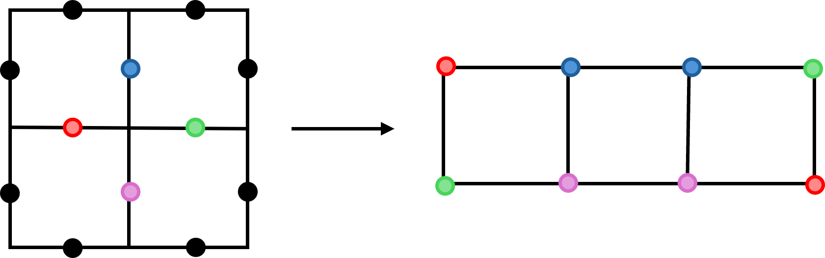
However, the Heisenberg bonds $\langle i,j\rangle$ form a bipartite edge graph (Fig. 1 (b)) and the coupling is antiferromagnetic ($J\geq 0$). Under these conditions, a Marshall sign transformation renders all off-diagonal elements non-positive, i.e., making the Hamiltonian stoquastic in this basis. As a result, the Perron-Frobenius theorem guarantees that the ground state can be chosen with non-negative amplitudes [7]. This substantially simplifies variational optimization: we may employ a positive real-valued NQS without learning a complex sign structure.

Let $\mathcal{E}=A\cup B$ be a partition of edges, $A\cap B=\varnothing$, chosen such that $A$ contains only dual-lattice edges and $B$ contains the direct-lattice edges, as illustrated in Fig. 1(b). We then define the Marshall transformation [54] as

$$U_{M}\coloneqq\prod_{i\in A}\sigma_{i}^{z}.$$ (16)

For any bond $\langle i,j\rangle$ with $i\in A,\ j\in B$, one finds

$$U_{M}(\sigma_{i}^{x}\sigma_{j}^{x})\,U_{M}^{\dagger} =-\sigma_{i}^{x}\sigma_{j}^{x},$$ (17)

$$U_{M}(\sigma_{i}^{y}\sigma_{j}^{y})\,U_{M}^{\dagger} =-\sigma_{i}^{y}\sigma_{j}^{y},$$ (18)

$$U_{M}(\sigma_{i}^{z}\sigma_{j}^{z})\,U_{M}^{\dagger} =\phantom{-}\sigma_{i}^{z}\sigma_{j}^{z},$$ (19)

while the stabilizers are invariant by construction,

$$U_{M}A_{v}U_{M}^{\dagger}=A_{v},\qquad U_{M}B_{p}U_{M}^{\dagger}=B_{p}.$$ (20)

Thus, the gauge-transformed Hamiltonian

$$H^{\prime} \coloneqq U_{M}HU_{M}^{\dagger}$$

$$=-\sum_{v}A_{v}-\sum_{p}B_{p}$$

$$\phantom{=}\;+J\sum_{\langle i,j\rangle}\bigl[-(\sigma_{i}^{x}\sigma_{j}^{x}+\sigma_{i}^{y}\sigma_{j}^{y})+\sigma_{i}^{z}\sigma_{j}^{z}\bigr]$$ (21)

is stoquastic in the $\sigma^{z}$ basis. Then, the ground state of $H^{\prime}$ can be chosen non-negative, and the ground state of the original $H$ has the Marshall sign structure

$$\psi(\sigma)=(-1)^{N_{\downarrow}(A;\sigma)}\,\phi(\sigma),\qquad\phi(\sigma)\geq 0,$$ (22)

where $N_{\downarrow}(A;\sigma)$ counts the number of down-spins on $A$ in configuration $\sigma$.

We next explain how to obtain the expectation value of observables in the physical gauge from the ground state in the Marshall gauge. Let the ground state of $H$ be $\ket{\psi_{phys}}$. Then the ground state in Marshall gauge can be expressed by $\ket{\psi_{M}}=U_{M}\ket{\psi_{\rm phys}}$ Since $U_{M}$ is unitary, any expectation value in the physical gauge follows from the Marshall gauge via

$$\langle O\rangle_{\rm phys}=\langle\psi_{M}|\,O_{M}\,|\psi_{M}\rangle,\qquad O_{M}\equiv U_{M}OU_{M}^{\dagger}.$$ (23)

With $U_{M}=\prod_{e\in A}\sigma^{z}_{e}$, one only needs an edgewise sign flip for $x/y$ on the $A$ sublattice:

$$U_{M}\sigma^{x,y}_{e}U_{M}^{\dagger}=\eta_{e}\,\sigma^{x,y}_{e},\quad U_{M}\sigma^{z}_{e}U_{M}^{\dagger}=\sigma^{z}_{e},$$ (24)

$$\eta_{e}=\begin{cases}-1,&e\in A,\\ +1,&e\in B.\end{cases}$$ (25)

II.3 Global Parity Symmetries and Logical Structure

We define the global spin-parity operators

$$P_{x}=\prod_{i}\sigma_{i}^{x},\qquad P_{z}=\prod_{i}\sigma_{i}^{z},$$ (26)

where the product runs over all spins residing on the edges of the square lattice. Because the star, plaquette, and bond operators include an even number of Pauli spin operators, one readily verifies

$$[H,P_{x}]=0,\qquad[H,P_{z}]=0.$$ (27)

Furthermore, for a two-atomic unit cell on an $L\times L$ torus, the total number of spins is $N=2L^{2}$, which is even. Thus, parity operators commute among themselves.

$$P_{x}P_{z}=(-1)^{N}P_{z}P_{x}=P_{z}P_{x}\quad\Rightarrow\quad[P_{x},P_{z}]=0.$$ (28)

These symmetries allow one to organize the Hilbert space into fixed $(P_{x},P_{z})$ sectors, which our neural-network ansatz explicitly targets. We note that the Heisenberg interaction preserves these global symmetries for all $J$, ensuring that total parity remains a robust quantum number. In contrast, the interaction does not commute with the non-contractible Wilson loops, meaning topological sectors are no longer conserved and their eigenvalues are hybridized by anyonic fluctuations. However, fixing the total parity has important consequences for the structure of the ground state space of the unperturbed toric code, which depends crucially on the lattice geometry. Since a non-contractible Wilson loop of Pauli type $\alpha\in\{x,z\}$ along direction $\gamma\in\{h,v\}$ is a product of $L$ single-spin operators, conjugation by the global parities gives

$$P_{x}\,W_{z}^{(\gamma)}\,P_{x} =(-1)^{L}\,W_{z}^{(\gamma)},$$ (29)

$$P_{z}\,W_{x}^{(\gamma)}\,P_{z} =(-1)^{L}\,W_{x}^{(\gamma)}.$$

In contrast, Wilson loops constructed from the same Pauli component as the parity operator commute trivially,

$$[P_{x},W_{x}^{(\gamma)}]=[P_{z},W_{z}^{(\gamma)}]=0,\qquad\gamma\in\{h,v\}.$$ (30)

For lattices with even $L$, the factor $(-1)^{L}=+1$. Therefore, all non-contractible Wilson loops commute with both parity operators,

$$[P_{x},W_{\alpha}^{(\gamma)}]=[P_{z},W_{\alpha}^{(\gamma)}]=0,\qquad(\text{even }L),$$ (31)

for all $\alpha\in\{x,z\}$ and $\gamma\in\{h,v\}$. Consequently, the ground state can be chosen as a simultaneous eigenstate of the Hamiltonian, all four non-contractible Wilson loops, and both total parity operators.

For lattices with odd $L$, the situation is qualitatively different. In this case, the cross-type pairs anticommute,

$$\{P_{x},W_{z}^{(\gamma)}\}=\{P_{z},W_{x}^{(\gamma)}\}=0,\qquad(\text{odd }L),$$ (32)

while $[P_{x},W_{x}^{(\gamma)}]=0$ and $[P_{z},W_{z}^{(\gamma)}]=0$ still hold. This algebraic structure implies that no state can be a simultaneous eigenstate of both the global parity operators and all logical Wilson loops. For example, let $\ket{w_{h},w_{v}}$ denote the common eigenbasis of the two $z$-type logical Wilson loops,

$$\begin{gathered}W_{z}^{(\gamma)}\ket{w_{h},w_{v}}=w_{\gamma}\,\ket{w_{h},w_{v}},\\ \gamma\in\{h,v\},\quad w_{h},w_{v}=\pm 1.\end{gathered}$$ (33)

Then, the eigenstate with $(p_{x},p_{z})=(-1,-1)$ can be chosen as

$$\ket{\Psi_{p_{x}=-1,\;p_{z}=-1}} =\frac{1}{\sqrt{2}}\Bigl(\ket{w_{h}=+1,\;w_{v}=-1}$$ (34)

$$\hskip 26.00009pt-\ket{w_{h}=-1,\;w_{v}=+1}\Bigr).$$

II.4 Variational Neural-Network Ansatz

To approximate the ground state of the Hamiltonian $H$, we employ a variational neural-network quantum state (NQS) that represents the many-body wave function $\psi(\sigma)$ in the computational ($\sigma^{z}$) basis. Since the Hamiltonian can be rendered stoquastic by a Marshall sign transformation, see Eq. (16), the ground-state amplitudes can be chosen real and non-negative. This allows us to focus exclusively on learning the amplitude structure of the wave function using a real-valued neural-network ansatz.

The network architecture is designed to exploit the physical symmetries of the lattice [49, 48, 11, 73]. We utilize translational symmetry via convolutional weight sharing, by mapping the edge-spin configuration onto a two-dimensional grid. A naive encoding, however, leads to unstable training, as star and plaquette couplings are distributed across distant grid locations [76]. We resolve this issue by introducing a geometry-aware positional embedding, which maps the four bonds incident on each vertex into local $2\times 4$ blocks. This construction, detailed in Appendix A, condenses the off-diagonal star operators into local features that can be efficiently processed by the network. To further restrict the variational space to physically relevant states, we explicitly enforce invariance under discrete $C_{4}$ lattice rotations. For a network that outputs the log-amplitude $\ell_{\theta}(\sigma)=\log\psi_{\theta}(\sigma)$, we define the $C_{4}$-symmetrized model as

$$\ell_{\theta}^{(C_{4})}(\sigma)=\log\!\left[\frac{1}{4}\sum_{k=0}^{3}\exp\!\left(\ell_{\theta}(\mathcal{R}^{k}\sigma)\right)\right],$$ (35)

where $\mathcal{R}$ denotes a $90^{\circ}$ rotation acting on the spin configuration. This symmetrization increases the computational cost but significantly reduces the effective variational search space and improves convergence toward the symmetric ground state [64, 80, 81, 62, 67, 55].

In practice, the network utilizes modern CNN techniques such as skip connections and increased cardinality to enhance expressivity while maintaining numerical stability, which are specified in Appendix A. To prevent divergence in the log-amplitudes as the system size increases, we employ normalized global aggregation layers. By construction, the resulting output is invariant under lattice translations by integer units of stars or plaquettes. To train the NQS, we employ a variational Monte Carlo (VMC) approach, the details of which are provided in Appendix B.

II.5 Parity on Marshall Gauge and Duality Constraints

Our variational ansatz is chosen to be even under a global spin flip in the $\sigma^{z}$ basis,

$$\psi(\{\sigma^{z}\})=\psi(\{-\sigma^{z}\})\quad\Longleftrightarrow\quad P_{x}|\psi\rangle=+|\psi\rangle.$$ (36)

The calculation is performed in the Marshall gauge, $H^{\prime}=U_{M}HU_{M}^{\dagger}$, under which the variational ground state is restricted to the $P_{x}=+1$ eigenspace of $H^{\prime}$. The corresponding physical expectation value follows from

$$U_{M}P_{x}U_{M}^{\dagger}=(-1)^{L^{2}}P_{x},$$ (37)

so that

$$\langle P_{x}\rangle_{\mathrm{phys}}=(-1)^{L^{2}}\,\langle P_{x}\rangle,$$ (38)

where the expectation value on the right-hand side is evaluated in the Marshall gauge.

For even $L$, the operator $P_{z}$ can be expressed as a product of plaquette operators, which fixes $P_{z}=+1$. For odd $L$, no such identity exists. Nevertheless, the Hamiltonian possesses an exact $x\!\leftrightarrow\!z$ duality. Let $H_{\rm ad}$ denote the single-qubit Hadamard operator,

$$H_{\rm ad}\sigma^{x}H_{\rm ad}=\sigma^{z},\quad H_{\rm ad}\sigma^{z}H_{\rm ad}=\sigma^{x},\quad H_{\rm ad}\sigma^{y}H_{\rm ad}=-\sigma^{y}.$$ (39)

Let $\mathcal{T}$ be the unitary operator implementing a one-site lattice translation,

$$\mathcal{T}\,\sigma_{e}^{\mu}\,\mathcal{T}^{\dagger}=\sigma_{\mathcal{T}(e)}^{\mu},$$ (40)

and define the duality operator

$$\mathcal{D}_{\rm dual}=\mathcal{T}\,(H_{\rm ad})^{\otimes N}.$$ (41)

Its action exchanges stars and plaquettes and maps

$$\mathcal{D}_{\rm dual}P_{z}\mathcal{D}_{\rm dual}^{\dagger}=P_{x}.$$ (42)

Since the Heisenberg interaction is invariant under this transformation,

$$[\mathcal{D}_{\rm dual},H]=0,$$ (43)

one expects $\langle P_{x}\rangle=\langle P_{z}\rangle$ in any finite-size system with a nondegenerate ground state. Combining this with the Marshall-Gauge relation yields

$$\langle P_{z}\rangle_{\mathrm{phys}}=(-1)^{L^{2}},$$ (44)

i.e., $\langle P_{z}\rangle_{\mathrm{phys}}=+1$ for even $L$ and $\langle P_{z}\rangle_{\mathrm{phys}}=-1$ for odd $L$. Since $P_{z}$ is not explicitly fixed within our variational ansatz, we introduce a weak guiding term that biases the optimization toward the appropriate parity sector, as detailed in Appendix B. We have verified this relation by exact diagonalization on $2\times 2$ and $3\times 3$ tori. Already for a very small Heisenberg coupling, $J=10^{-4}$, the finite-size ground state lies in the parity sector consistent with $\langle P_{x}\rangle_{\mathrm{phys}}=\langle P_{z}\rangle_{\mathrm{phys}}=(-1)^{L^{2}}$.

II.6 Observables for the detection of the quantum phase transition

In this subsection, we explain the observables used to detect phase transitions and determine the phase after the transition.

We evaluate the ground-state fidelity between the states at $J$ and $J+\delta J$,

$$F(J,J+\delta J)\equiv\bigl|\langle\psi_{M}(J)\mid\psi_{M}(J+\delta J)\rangle\bigr|^{2},$$ (45)

and estimate the fidelity susceptibility from the small-$\delta J$ expansion

$$F(J,J+\delta J)=1-\chi_{F}(J)(\delta J)^{2}+\mathcal{O}\!\left((\delta J)^{3}\right).$$ (46)

In practice, we assign the estimate to the midpoint

$$J_{\rm mid}\equiv J+\frac{\delta J}{2},$$ (47)

and use the finite-difference formula

$$\chi_{F}(J_{\rm mid})\approx\frac{\,[1-F(J,J+\delta J)]}{(\delta J)^{2}}.$$ (48)

For a continuous quantum phase transition, $\chi_{F}$ obeys the finite-size scaling form

$$\chi_{F}(J,L)=L^{2/\nu}\,\Phi\!\bigl((J-J_{c})L^{1/\nu}\bigr),$$ (49)

where $\nu$ is the correlation-length exponent [90, 89, 2, 87, 20]. Equation (49) implies that the peak height scales as

$$\chi_{F}^{\max}(L)\propto L^{2/\nu},$$ (50)

while the peak position $J^{*}(L)$ drifts towards the thermodynamic critical point $J_{c}$ as

$$J^{*}(L)-J_{c}\propto L^{-1/\nu}.$$ (51)

In Sec. IV, we utilize these relations to extract $\nu$ from the peak height and estimate $J_{c}$ via the peak shift using Eq. (51).

To complement the fidelity-based analysis with a diagnostic that directly probes the nonlocal topological content of the ground state, we introduce

$$\begin{split}\bar{W}_{d}(J,L)&=\frac{1}{2}\Bigl(\bigl|\langle W_{x}^{(h)}W_{x}^{(v)}\rangle_{\mathrm{phys}}\bigr|\\ &\quad+\bigl|\langle W_{z}^{(h)}W_{z}^{(v)}\rangle_{\mathrm{phys}}\bigr|\Bigr).\end{split}$$ (52)

Deep in the topological phase, $\bar{W}_{d}$ remains of order unity, although its baseline value differs between odd and even $L$: for odd $L$, both loop products approach $-1$ in magnitude (see, Eq. (72)), giving $\bar{W}_{d}\simeq 1$, whereas for even $L$ they take values slightly larger than $1/2$, giving $\bar{W}_{d}\simeq 0.5$–$0.6$ (see, Eq. (75)). This parity-dependent baseline is a finite-size effect originating from the interplay between global parity constraints and the non-contractible Wilson loop algebra, and is discussed in Sec. III.4. Beyond the transition, the non-contractible loop expectation values are exponentially suppressed in $L$, so $\bar{W}_{d}\to 0$ as $L\to\infty$ in the trivial phase. To locate the steepest decay of topological order, we monitor the logarithmic susceptibility

$$\chi_{W}^{(\ln)}(J,L)\;=\;-\frac{d\ln\bar{W}_{d}}{dJ}\,,$$ (53)

which we evaluate numerically via finite differences. We adopt the logarithmic form to measure the relative rate of change, which is insensitive to the parity-dependent baseline. This yields peak positions providing a robust nonlocal estimate of the critical coupling that complements the fidelity-susceptibility analysis.

In addition, we compute the second Rényi entropy $S_{2}(R)$ of subsystems $R$ using a replica (SWAP) estimator and extracting the topological constant via the Kitaev–Preskill (KP) construction [40, 22]. For three adjacent regions $A,B,C$ each forming a simply connected patch, the KP combination

$$\begin{split}\gamma_{\mathrm{KP}}\equiv{}&S_{2}(A)+S_{2}(B)+S_{2}(C)\\ &-S_{2}(AB)-S_{2}(BC)-S_{2}(CA)\\ &+S_{2}(ABC)\end{split}$$ (54)

is designed to cancel all boundary-law contributions $\alpha|\partial R|$ as well as corner-dependent and other local short-range terms, leaving only the universal $O(1)$ constant associated with long-range entanglement. With this convention, the $\mathbb{Z}_{2}$ topologically ordered phase is characterized by a constant topological entanglement entropy $\gamma_{\mathrm{KP}}=-\ln 2$ in the thermodynamic limit. Beyond the topological transition, conventional order may emerge. In a finite system without an explicit symmetry-breaking field, the ground state can remain symmetry-preserving and effectively form a superposition over symmetry-related configurations [3]. For broken discrete symmetries with degeneracy $d$, this sector mixing contributes an additive Shannon-like term $+\ln d$ to the entanglement entropy (opposite in sign to the topological reduction), which does not necessarily cancel in the Kitaev–Preskill subtraction and can therefore yield an apparent $\gamma_{\mathrm{KP}}>0$ even in a topologically trivial ordered regime [30, 72, 37]. Moreover, at intermediate lattice sizes, the entanglement-entropy extraction can be contaminated by non-universal finite-size effects (e.g., when the correlation length is comparable to the linear size of the subregions). Hence, conventional order in finite size system can lead to an intrinsically ambiguous residual nonzero $\gamma_{\mathrm{KP}}$ in the non-topological regime [88, 42, 72, 34]. Furthermore, we note that fidelity and topological entanglement entropy(TEE) are invariant under the Marshall gauge, $U_{M}$; inner products are preserved, and Rényi-2 entropies from the swap estimator are unchanged because local unitaries on a region commute with the swap operator. Finally, to analyze conventional antiferromagnetic order, we use the Marshall-transformation adapted staggered magnetization:

$$m_{\alpha}^{\mathrm{stag}} =\frac{1}{N}\sum_{i}\eta_{i}\,\sigma_{i}^{\alpha},\qquad\alpha\in\{x,y,z\},$$ (55)

$$\eta_{i} =$$

III Schrieffer-Wolff transformation

The SW transformation is a canonical unitary approach for deriving effective low-energy descriptions of quantum many-body systems, which have been successfully applied for condensed matter physics [82, 33, 28, 52] and quantum information theory [4, 58, 59, 5, 50, 24, 36, 91, 12, 92, 53]. Given a Hamiltonian with a clear separation of energy scales, the SW procedure constructs a unitary rotation $e^{S}$ that block-diagonalizes the perturbed Hamiltonian with respect to a chosen low-energy subspace, thereby integrating out virtual transitions to high-energy sectors and producing an effective Hamiltonian acting within the low-energy manifold [6, 69, 38, 27, 63, 83, 43].

In our setting, the Heisenberg exchange does not commute with the toric-code stabilizers and thus couples the ground-state manifold to sectors with virtual $e$ and $m$ anyons. We apply the SW transformation in the projector formalism [6] to derive the effective Hamiltonian on the stabilizer ground state space, integrating out these virtual anyon processes order by order. This yields a controlled expansion of the effective Hamiltonian and explicitly identifies the operator contributions arising at each perturbative order. In the following, we present the resulting effective Hamiltonian and show that the leading orders merely renormalize the star and plaquette terms, while mixing of topological sectors appears only at order $L$, i.e., at a perturbative order proportional to the system size. Our results are consistent with earlier work that finds topological-sector mixing exponentially small in $L$, and further clarify how a local perturbation dress stabilizers and Wilson loops in the effective theory. In addition, we analyze how the parity of the lattice size $L$ influences the finite-size ground-state selection and lifts the degeneracy differently for even and odd systems. Detailed derivations are provided in Appendix C.

III.1 Model and SW setup

We split the Hamiltonian as

$$H_{0}^{SW} =-J_{e}\sum_{v}A_{v}-J_{m}\sum_{p}B_{p},$$ (56)

introducing independent positive coupling constants $J_{e}$ and $J_{p}$ for the star and plaquette operators. The isotropic antiferromagnetic Heisenberg perturbation on the edge graph with coupling $J\geq 0$ is given by

$$V =J\sum_{b=\langle i,j\rangle}\bigl(X_{b}+Y_{b}+Z_{b}\bigr),$$ (57)

$$X_{b} =\sigma^{x}_{i}\sigma^{x}_{j},\quad Y_{b}=\sigma^{y}_{i}\sigma^{y}_{j},\quad Z_{b}=\sigma^{z}_{i}\sigma^{z}_{j}.$$

Acting once with these bond operators creates two-anyon excitations with gaps

$$\Delta_{x} =4J_{m},$$ (58)

$$\Delta_{z} =4J_{e},$$

$$\Delta_{y} =4(J_{e}+J_{m}).$$

We thus identify the controlled-expansion regime as $J\ll\min(4J_{m},4J_{e})$.

III.2 Projector–resolvent form of the Schrieffer–Wolff generator

We briefly summarize the standard SW construction in the projector-resolvent language [6].

Let $P$ project onto the unperturbed code space and $Q=\mathbf{1}-P$ onto its orthogonal complement. We seek an anti-Hermitian generator $S^{\dagger}=-S$ such that the rotated Hamiltonian $\tilde{H}\equiv e^{S}H^{\rm SW}e^{-S}$ is block diagonal, effectively decoupling the $P$ and $Q$ subspaces order by order in the perturbation strength. Working in the off-diagonal gauge

$$PSP=QSQ=0,$$ (59)

and expanding $S=S_{1}+\mathcal{O}(J^{2})$, the first-order generator can be written compactly in terms of the reduced resolvent

$$R\equiv Q\,(E_{P}-H_{0}^{\rm SW})^{-1}Q,\qquad PR=RP=0,$$ (60)

as

$$S_{1}=PVR-RVP,$$ (61)

which cancels the $\mathcal{O}(J)$ mixing between $P$ and $Q$. Projecting onto $P$ gives

$$\begin{split}H_{\rm eff}&\equiv P\,e^{S}(H_{0}^{\rm SW}+V)e^{-S}P\\ &=P(H_{0}^{\rm SW}+V)P+\mathcal{O}(J^{2}).\end{split}$$ (62)

For the present Heisenberg perturbation, a single bond creates stabilizer defects, hence $PVP=0$ and the first-order correction vanishes:

$$H_{\rm eff}=PH_{0}^{\rm SW}P+\mathcal{O}(J^{2}).$$ (63)

III.3 Effective Hamiltonian to $\mathcal{O}(J^{2})$

The leading nontrivial contribution to $H_{\rm eff}$ arises at second order. Using the SW expansion with the generator in Eq.(61), we find an $\mathcal{O}(J^{2})$ correction controlled by two-bond virtual processes. The projected effective Hamiltonian through $\mathcal{O}(J^{2})$ is

$$\begin{split}H_{\rm eff}={}&P\biggl[-\Bigl(J_{e}+\frac{J^{2}}{J_{m}}\Bigr)\sum_{v}A_{v}-\Bigl(J_{m}+\frac{J^{2}}{J_{e}}\Bigr)\sum_{p}B_{p}\\ &\quad+E_{\rm const}^{(2)}\biggr]P+\mathcal{O}(J^{3})\end{split}$$ (64)

with a second-order constant shift

$$E_{\mathrm{const}}^{(2)}=-\,L^{2}J^{2}\left(\frac{1}{J_{m}}+\frac{1}{J_{e}+J_{m}}+\frac{1}{J_{e}}\right).$$ (65)

Since $P$ projects onto the code space where $A_{v}=B_{p}=+1$, $PH_{\rm eff}P$ reduces to an overall energy shift within the ground space sector up to second order. Specifically, on an $L\times L$ torus, there are $L^{2}$ vertex stabilizers $A_{v}$ and $L^{2}$ plaquette stabilizers $B_{p}$, while the total number of spins is $N=2L^{2}$. Hence, the energy per spin becomes

$$\frac{E_{0}(J)}{N} =-\frac{J_{e}+J_{m}}{2}-\frac{J^{2}}{2}\left[\frac{2}{J_{m}}+\frac{2}{J_{e}}\right.$$ (66)

$$\qquad\left.+\frac{1}{J_{e}+J_{m}}\right]+\mathcal{O}(J^{3}),$$

which is independent of $L$ up to second order. For the choice $J_{e}=J_{m}=1$, Eq. (66) reduces to

$$\frac{E_{0}(J)}{N}=-1-\frac{9}{4}J^{2}+\mathcal{O}(J^{3}).$$ (67)

III.4 Higher-order SW terms and logical-operator effective theory

Beyond second order, the SW expansion generates a hierarchy of gauge-invariant operator structures built from connected strings of perturbations and reduced resolvents. After projection onto the toric-code ground space, products of local stabilizers—equivalently, any contractible loop operators—act as constants and can therefore be absorbed into an overall energy shift. Consequently, the operator contents that remain qualitatively relevant for topological-sector splitting on the torus are those involving non-contractible Wilson loops and firstly appear at $L$-th order.

While an $L\times L$ torus admits $L$ distinct straight paths for each winding direction $\gamma\in\{h,v\}$ and Pauli type $\alpha\in\{x,z\}$, these operators are not independent. One can define $L$ representatives $W_{\alpha}^{(\gamma)}(r)$ by translating a loop transversally by $r$ lattice units; however, all these loops operators are the same up to multiplication by contractible strips generated by $\{A_{v}\}$ and $\{B_{p}\}$. Since the projector $P$ enforces $A_{v}=B_{p}=+1$ in the toric-code ground space, such contractible factors act trivially after projection, and all translated representatives act identically within the code space:

$$P\,W_{\alpha}^{(\gamma)}(r)\,P=P\,W_{\alpha}^{(\gamma)}(r^{\prime})\,P,\qquad\forall\,r,r^{\prime}.$$ (68)

We may therefore drop the transverse label and define the corresponding code-space winding operator as

$$W_{\alpha}^{(\gamma)}\;\equiv\;P\,W_{\alpha}^{(\gamma)}(r_{0})\,P\;=\;\frac{1}{L}\,P\Big(\sum_{r=1}^{L}W_{\alpha}^{(\gamma)}(r)\Big)P,$$ (69)

for any fixed representative $r_{0}$. The normalization ensures eigenvalues $\pm 1$ in the ground space (matching a logical Pauli operator), while the translation-average on the right-hand side makes the underlying symmetry manifest and is often convenient in numerical measurements. Importantly, loops winding along $h$ and $v$ remain independent logical operators on the torus.

At the dual point $J_{e}=J_{m}=1$, the requirements of hermiticity, $C_{4}$ rotational symmetry, and duality restrict the most general effective Hamiltonian to the simpler form. The resulting operator content is subject to an even–odd selection rule: for odd $L$, the global parities $P_{x}$ and $P_{z}$ forbid all terms linear in a single winding loop. For even $L$, however, such single-loop terms are allowed and appear at the $L$-th order. Using Eq. (12), the general effective Hamiltonian can be written as

$$H_{\rm eff}^{\rm odd} =c_{0}\,P+P\Bigl[u\bigl(\bar{X}_{1}\bar{X}_{2}+\bar{Z}_{1}\bar{Z}_{2}\bigr)+w\,\bar{Y}_{1}\bar{Y}_{2}\Bigr]P,$$ (70)

$$H_{\rm eff}^{\rm even} =c_{0}\,P+P\Bigl[t\bigl(\bar{X}_{1}+\bar{X}_{2}+\bar{Z}_{1}+\bar{Z}_{2}\bigr)$$

$$\qquad+u\bigl(\bar{X}_{1}\bar{X}_{2}+\bar{Z}_{1}\bar{Z}_{2}\bigr)$$

$$\qquad+v\bigl(\bar{X}_{1}\bar{Z}_{2}+\bar{Z}_{1}\bar{X}_{2}\bigr)+w\,\bar{Y}_{1}\bar{Y}_{2}\Bigr]P,$$

where $\bar{Y}_{j}\equiv i\bar{X}_{j}\bar{Z}_{j}$. All logical couplings are generated by winding (and higher-order connected) virtual processes and scale parametrically as $t,u,v,w=\mathcal{O}\!\left(J^{L}/\Delta^{L-1}\right)$ in the topological regime.

For odd $L$, the single winding loops are odd under the conserved global parities $P_{x}$ and $P_{z}$, hence all single-loop expectation values vanish in any fixed $(P_{x},P_{z})$ block,

$$\langle\bar{X}_{1}\rangle=\langle\bar{X}_{2}\rangle=\langle\bar{Z}_{1}\rangle=\langle\bar{Z}_{2}\rangle=0\qquad(L\ \text{odd}).$$ (71)

The leading dynamics in $H_{\rm eff}^{\rm odd}$ is therefore governed by the commuting two-qubit operators $\bar{X}_{1}\bar{X}_{2}$, $\bar{Z}_{1}\bar{Z}_{2}$, and $\bar{Y}_{1}\bar{Y}_{2}$. Moreover, it turns out that $u>0$ and $w>0$ while $|w|\ll|u|$ for odd L (Appendix C.6). This selects a Bell-type ground state in the ground space, which implies the characteristic loop pattern

$$\begin{aligned} \langle W_{x}^{(h)}W_{x}^{(v)}\rangle&\simeq-1,\\ \langle W_{z}^{(h)}W_{z}^{(v)}\rangle&\simeq-1,\end{aligned}\qquad(L\ \text{odd},\ J\ll J_{c})$$ (72)

together with Eq. (71). Thus, odd-$L$ systems naturally realize a cat-state structure with strong sector mixing even deep within the topological regime: Expectation values of single winding loops vanish, while parity-even loop products attain degenerate, maximally negative values.

In the intermediate size of even-$L$ case, the hierarchy $|t|\gtrsim|u|\gg|v|,|w|$ is maintained, with all four coefficients taking negative values (Appendix C.6). When the coefficient $t$ dominates, the leading contribution is a single-qubit logical field proportional to $\bar{X}+\bar{Z}$ on each logical qubit. The corresponding ground state is approximately polarized along the bisector of the $\bar{X}$ and $\bar{Z}$ axes, giving

$$\begin{aligned} \langle\bar{X}_{1}\rangle\simeq\langle\bar{X}_{2}\rangle&\simeq\frac{1}{\sqrt{2}},\\ \langle\bar{Z}_{1}\rangle\simeq\langle\bar{Z}_{2}\rangle&\simeq\frac{1}{\sqrt{2}},\end{aligned}\qquad(L\ \text{even},\ J\ll J_{c}).$$ (73)

i.e.,

$$\langle W_{x}^{(h)}\rangle\simeq\langle W_{x}^{(v)}\rangle\simeq\langle W_{z}^{(h)}\rangle\simeq\langle W_{z}^{(v)}\rangle\simeq\frac{1}{\sqrt{2}}.$$ (74)

The remaining couplings $u,v,w$ act as subleading two-qubit interactions that correlate the logical qubits and shift these expectations away from the ideal bisector values. Specifically, the same dominant-bisector picture predicts the baseline $\langle W_{x}^{(h)}W_{x}^{(v)}\rangle\approx\langle W_{x}^{(h)}\rangle\langle W_{x}^{(v)}\rangle\simeq 1/2$ (and similarly for $z$) if the two logical qubits were independent. In practice, however, the two-qubit logical interactions—most importantly the $u(\bar{X}_{1}\bar{X}_{2}+\bar{Z}_{1}\bar{Z}_{2})$ term—favor correlated responses of the two winding directions and thus enhance the products above this uncorrelated value,

$$\langle W_{x}^{(h)}W_{x}^{(v)}\rangle,\ \langle W_{z}^{(h)}W_{z}^{(v)}\rangle\;\gtrsim\;\frac{1}{2}\qquad(L\ \text{even},\ J\ll J_{c}).$$ (75)

Furthermore, since all logical couplings are tunneling-generated at order $L$, the overall topological splitting scale $\Delta E_{\rm topo}(L,J)\sim\mathcal{O}(J^{L}/\Delta^{L-1})$ becomes exponentially small at weak $J$. Strictly speaking, at any fixed finite system size the ground state is unique and must respect all symmetries of the Hamiltonian; it is therefore a symmetric superposition of the four logically polarized torus sectors rather than a symmetry-broken sector state. In the thermodynamic limit, the tunneling-induced splittings vanish and this near-degeneracy becomes an exact degeneracy such that any one of the symmetry-broken (sector-polarized) states can be selected as a legitimate ground state.

III.5 Dressed stabilizers $B_{p}$,$A_{v}$ and non-contractible Wilson loops

We can obtain dressed observables by applying the same SW unitary transformation,

$$O^{\rm eff}\equiv P\,e^{S}O\,e^{-S}P.$$ (76)

At order $\mathcal{O}(J^{2})$, the plaquette and star operators remain purely multiplicatively renormalized (no operator mixing within $P$ at this order). Using the excitation gaps $\Delta_{x},\Delta_{y},\Delta_{z}$, the dressed stabilizers read

$$B_{p}^{\rm eff} =\Bigl[1-32\bigl(\tfrac{J}{\Delta_{x}}\bigr)^{2}-16\bigl(\tfrac{J}{\Delta_{y}}\bigr)^{2}\Bigr]\,PB_{p}P+\mathcal{O}(J^{3})$$

$$=\Bigl[1-2\Bigl(\tfrac{J}{J_{m}}\Bigr)^{2}-\Bigl(\tfrac{J}{J_{e}+J_{m}}\Bigr)^{2}\Bigr]\,PB_{p}P+\mathcal{O}(J^{3}),$$ (77)

$$A_{v}^{\rm eff} =\Bigl[1-32\bigl(\tfrac{J}{\Delta_{z}}\bigr)^{2}-16\bigl(\tfrac{J}{\Delta_{y}}\bigr)^{2}\Bigr]\,PA_{v}P+\mathcal{O}(J^{3})$$

$$=\Bigl[1-2\Bigl(\tfrac{J}{J_{e}}\Bigr)^{2}-\Bigl(\tfrac{J}{J_{e}+J_{m}}\Bigr)^{2}\Bigr]\,PA_{v}P+\mathcal{O}(J^{3}).$$ (78)

Furthermore, We define dressed shortest non-contractible Wilson loop operators by

$$W^{\rm eff}_{z/x}(C)\equiv P\,e^{S}W_{z/x}(C)\,e^{-S}P,$$ (79)

where $C$ is a straight winding cycle of length $L$. At $\mathcal{O}(J^{2})$ the projection again yields a purely multiplicative renormalization. For $W_{z}(C)=\prod_{e\in C}\sigma^{z}_{e}$ one finds

$$PW^{\rm eff}_{z}(C)P =\Bigl[1-6L\bigl(\tfrac{J}{\Delta_{x}}\bigr)^{2}-8L\bigl(\tfrac{J}{\Delta_{y}}\bigr)^{2}\Bigr]$$ (80)

$$\qquad\times PW_{z}(C)P+\mathcal{O}(J^{3}),$$

while for $W_{x}(C)=\prod_{e\in C}\sigma^{x}_{e}$,

$$PW^{\rm eff}_{x}(C)P =\Bigl[1-6L\bigl(\tfrac{J}{\Delta_{z}}\bigr)^{2}-8L\bigl(\tfrac{J}{\Delta_{y}}\bigr)^{2}\Bigr]$$ (81)

$$\qquad\times PW_{x}(C)P+\mathcal{O}(J^{3}).$$

IV Numerical Results for the Ground State

Figure 2: Ground state energy per spin $E_{0}/N$ (with $N=2L^{2}$) versus the AFM Heisenberg coupling $J$ for $L=3,4,5,6$. Symbols show NQS results and error bars represent stochastic uncertainty; for $L=3$ we also plot the exact-diagonalization (ED) benchmark. The dashed curve is the SW prediction truncated at $\mathcal{O}(J^{2})$, see Eq. (67). Note that this approximation coincides with the result up to third order for $L\geq 4$; see Appendix C.5. In the perturbative regime $J\lesssim 0.1$, SW is in quantitative agreement with NQS/ED. For $J\gtrsim 0.13$–$0.16$, systematic deviations from the $\mathcal{O}(J^{2})$ curve appear and the $L$-dependence increases, consistent with the breakdown of low-order perturbation theory and the approach to the critical region.

Figure 3: Fidelity susceptibility $\chi_{F}$ obtained from NQS for $L=3,4,5,6$ and from ED for $L=3$. Prominent peaks indicate a phase crossover in this range of $J$. The peak height increases with system size $L$, while the peak position exhibits a slight finite-size drift.

\begin{overpic}[width=433.62pt,height=153.99933pt,keepaspectratio]{estimate_p.png} \put(2.0,87.0){(a)} \end{overpic}

\begin{overpic}[width=433.62pt,height=153.99933pt,keepaspectratio]{fidsus_jc.png} \put(2.0,87.0){(b)} \end{overpic}

Figure 4: Finite-size scaling analysis of the fidelity-susceptibility peak. (a) Log–log plot of the peak height, $\chi_{F}^{\mathrm{peak}}(L)$, versus $L$. From a linear fit, we obtain the critical exponent from $2/\nu=2.85\pm 0.54$. (b) Extrapolated critical coupling $J_{c}(\infty)$, obtained from the drift of the peak position by fitting $J_{\mathrm{peak}}(L)=J_{c}(\infty)+a/L^{1/\nu}$, shown as a function of the assumed shift exponent $1/\nu$. we obtained $a=-0.086$ in our fitting. The vertical dashed lines indicate the value of $1/\nu$ from (a), and the horizontal dashed line and band marks the corresponding $J_{c}=0.1641^{+0.0034}_{-0.0024}$. The blue vertical band indicates the uncertainty range of $1/\nu$ from (a).

\begin{overpic}[width=433.62pt,height=153.99933pt,keepaspectratio]{33XdZd.png} \put(0.0,85.0){(a)} \end{overpic}

\begin{overpic}[width=433.62pt,height=153.99933pt,keepaspectratio]{55XdZd.png} \put(0.0,85.0){(b)} \end{overpic}

Figure 5: Logical-qubit diagnostics from non-contractible Wilson loops for odd $L$. Shown are the parity-even double-winding correlators $\langle W_{x}^{(h)}W_{x}^{(v)}\rangle_{\rm phys}$ and $\langle W_{z}^{(h)}W_{z}^{(v)}\rangle_{\rm phys}$ for (a) $L=3$ and (b) $L=5$. Their deviation from the ideal toric-code values directly quantifies correlated logical errors induced by the isotropic Heisenberg interaction. Markers show NQS results for $L=3,5$, including the sampling/optimization uncertainty, as well as ED results for $L=3$. Dashed curves correspond to the $\mathcal{O}(J^{2})$ SW dressing of the logical correlators; good agreement at small $J$ validates the perturbative error model, while the rapid change and strong deviations near the transition region indicate the onset of the breakdown of the topological protection as the system crosses into the Néel-ordered phase.

\begin{overpic}[width=82.8019pt]{44XdZd.png} \put(0.0,82.0){\small(a)} \end{overpic}

\begin{overpic}[width=82.8019pt]{44XhZh.png} \put(0.0,82.0){\small(b)} \end{overpic}

\begin{overpic}[width=82.8019pt]{66XdZd.png} \put(0.0,82.0){\small(c)} \end{overpic}

\begin{overpic}[width=82.8019pt]{66XhZh.png} \put(0.0,82.0){\small(d)} \end{overpic}

Figure 6: Wilson-loop observables versus Heisenberg coupling $J$ for $L=4$ (a,b) and $L=6$ (c,d). (a,c) Double-winding products $\langle W_{x}^{(h)}W_{x}^{(v)}\rangle_{\rm phys}$ and $\langle W_{z}^{(h)}W_{z}^{(v)}\rangle_{\rm phys}$; (b,d) single-winding loops $\langle W_{x}^{(h)}\rangle_{\rm phys}$ and $\langle W_{z}^{(h)}\rangle_{\rm phys}$. A small-$J$ plateau near the perturbative reference values (dashed: $0.5$ and $1/\sqrt{2}$) marks the topological regime, while the pronounced drop with $J$ signals the approach to a topological phase transition and increased logical error propensity. Because of the near-degeneracy for even L discussed in Appendix D, they show slight deviation from the duality.

\begin{overpic}[width=433.62pt,height=153.99933pt,keepaspectratio]{Wd_bar.png} \put(-2.0,82.0){(a)} \end{overpic}

\begin{overpic}[width=433.62pt,height=153.99933pt,keepaspectratio]{chi_W_log.png} \put(-2.0,82.0){(b)} \end{overpic}

Figure 7: Composite non-contractible Wilson-loop diagnostic $\bar{W}_{d}$, defined in Eq. (52), for $L=3,4,5,6$ (ED for $3\times 3$; NQS for all sizes). (a) $\bar{W}_{d}(J,L)$ remains close to its baseline in the topological phase and undergoes a pronounced suppression toward zero as $J$ increases, with the decay becoming steeper for larger system sizes within the same even- or odd-$L$ sector. The even/odd-dependent baseline differs between odd $L$ ($\bar{W}_{d}\simeq 1$) and even $L$ ($\bar{W}_{d}\simeq 0.5$–$0.6$), consistent with the finite-size structure discussed in Sec. III.4. The vertical dashed line marks the estimated critical coupling $J_{c}\approx 0.164$. (b) The logarithmic susceptibility $\chi_{W}^{(\ln)}$ exhibits a peak that sharpens and grows with increasing $L$, signaling the breakdown of topological order. Because of the even/odd dependence on $L$, the peak heights follow separate even and odd branches—$\chi_{W}^{(\mathrm{ln},\mathrm{peak})}(L{=}3)<\chi_{W}^{(\mathrm{ln},\mathrm{peak})}(L{=}5)$ and $\chi_{W}^{(\mathrm{ln},\mathrm{peak})}(L{=}4)<\chi_{W}^{(\mathrm{ln},\mathrm{peak})}(L{=}6)$—while even and odd $L$ may alternate in magnitude at comparable system sizes. The peak positions are located near $J_{c}\simeq 0.164$, consistent with the fidelity susceptibility analysis.

Figure 8: Kitaev–Preskill topological entanglement indicator $\gamma_{\rm KP}$, extracted from the second Rényi entropies for the ground state of the toric code with AFM Heisenberg coupling $J$. Results are shown for system sizes $L=3-6$, obtained via NQS (We also include ED results for benchmarking). We use the convention $\gamma_{\rm KP}\equiv S(A)+S(B)+S(C)-S(AB)-S(BC)-S(CA)+S(ABC)$. Thus, an ideal $\mathbb{Z}_{2}$ topological phase yields $\gamma_{\rm KP}=-\ln 2$ (dotted line). As $J$ increases, $\gamma_{\rm KP}$ rises toward zero, signaling the loss of topological order. For larger $J$, $\gamma_{\rm KP}$ becomes positive because of the contribution from cat state mixing and finite size effect; this induces a Shannon-like mixing contribution to the Rényi entropies that is not removed by the KP subtraction.

In this section, we show our numerical results. All expectation values in this section are calculated in the physical basis, see Eq. (23).

We begin with a benchmark of our methodologies in the perturbative regime and present results that support the accuracy of our NQS ansatz and the validity of the SW expansion. Figure 2 compares the ground-state energies per spin for $L=3,4,5,6$ and the SW effective Hamiltonian up to second order. We furthermore include the ED result for $3\times 3$. In the small-$J$ regime, the SW results agree quantitatively with the NQS energies, confirming the controlled nature of the expansion and the accuracy of the NQS. As $J$ increases, deviations gradually develop, and the variational NQS energy becomes systematically lower than the SW estimate, signaling the breakdown of the perturbative description.

Next, we show the fidelity susceptibility $\chi_{F}$ for $L=3,4,5,6$ in Fig. 3, which exhibits a pronounced peak that sharpens and drifts slightly toward larger $J$ as $L$ increases. By performing a finite-size scaling analysis of the peak heights and positions, see Eq. (50) and Eq. (51), we extrapolate the transition point in the thermodynamic limit, as shown in Fig. 4. This analysis yields $J_{c}\simeq 0.164$ within the grid error.

We next present the numerical data for the non-contractible Wilson-loop expectation values. For odd $L$, symmetry constraints enforce $\langle W_{x}\rangle_{\mathrm{phys}}=\langle W_{z}\rangle_{\mathrm{phys}}=0$, as discussed in Sec. II.3, which implies strong mixing between topological sectors. On the other hand, the parity-even double-winding operators

$$W_{z}^{(h)}W_{z}^{(v)},\qquad W_{x}^{(h)}W_{x}^{(v)},$$ (82)

commute with both $P_{x}$ and $P_{z}$ even for odd $L$ and are thus not forbidden by symmetry. The results for odd $L$ are presented in Fig. 5. The parity-even double-winding operators take negative expectation values, in excellent agreement with our SWT predictions. For odd system sizes and $J=0$, the global parity operators $P_{x}$ and $P_{z}$ coincide with the double-winding operators $W_{x}^{(h)}W_{x}^{(v)}$ and $W_{z}^{(h)}W_{z}^{(v)}$, respectively. This follows because each parity operator can be decomposed into the product of double-winding operators and a set of contractible loops; the latter are products of local stabilizers $A_{v}$ or $B_{p}$, which evaluate to $+1$. To minimize the total energy for $J>0$, the ground state naturally resides in the $P_{x}=P_{z}=-1$ sector, which is in agreement with Eq. (38) and Eq. (44). In this regime, the magnitudes of these loop expectation values increase gradually and remain well captured by the perturbative SW results. As the system approaches the transition region, however, we observe a markedly sharper increase together with substantial deviations from the SWT curves, signaling the breakdown of the low-order effective description. Beyond the transition, the data suggest a gradual evolution toward smaller values, consistent with the loss of topological protection and the accompanying decay of non-local correlations.

Next, we examine the non-contractible Wilson loop data for even lattice sizes ($L=4,6$) shown in Fig. 6. In the weak-coupling regime, the single-loop expectation values in the $x$ and $z$ channels remain close to the duality-symmetric value of $1/\sqrt{2}$. This confirms that the optimized finite-size ground state respects the Hamiltonian duality. Furthermore, the loop products systematically exceed the independent-qubit baseline of $1/2$, suggesting the presence of correlations between the logical sectors that are not captured by the simple mixing as predicted in Sec. C.6. We note that for very small $J$, the topological energy splitting $\Delta E_{\rm topo}\sim J^{L}/\Delta^{L-1}$ becomes so small that the variational optimization may converge to metastable, logically polarized states rather than the duality-symmetric ground state. In such states, the ansatz effectively polarizes into one Wilson-loop type, e.g. $\langle W_{x}\rangle\gg\langle W_{z}\rangle$ or vice versa, thereby appearing to break the expected duality at finite size, see Appendix D.

We can now use the non-contractible Wilson-loop data to build an indicator for the topological phase transition and to complement the fidelity-based estimate. We use the composite non-contractible Wilson-loop indicator $\bar{W}_{d}(J,L)$ defined in Eq. (52). As shown in Fig. 7(a), the suppression of $\bar{W}_{d}$ with increasing $J$ becomes progressively steeper for larger system sizes, consistent with a sharpening phase transition. To locate the coupling at which the topological order decays most rapidly, we monitor the logarithmic susceptibility $\chi_{W}^{(\ln)}=-d\ln\bar{W}_{d}/dJ$ [Eq. ((52))], which measures the relative rate of change and is thereby insensitive to the even-odd-dependent baseline. As shown in Fig. 7(b), $\chi_{W}^{(\ln)}$ develops a peak that sharpens and grows with $L$, with peak positions being located near $J_{c}\simeq 0.164$, providing a nonlocal estimate of the critical coupling that is fully consistent with the fidelity susceptibility analysis. We note that at comparable system sizes, even-$L$ systems exhibit systematically larger peak heights than odd-$L$ systems. This is attributed to the different baseline structures between even and odd $L$.

Having established the transition point and the role of even/odd L dependence of the non-contractible Wilson loop operators, we next examine the TEE, $\gamma_{\mathrm{KP}}$ (Fig. 8). We find that the regime where the SW energy predictions begin to deviate from our numerical results coincides precisely with the rapid growth of the fidelity susceptibility and the departure of $\gamma_{\mathrm{KP}}$ from its unperturbed topological value of $-\ln 2$. The peak in $\chi_{F}$ and the simultaneous crossover in $\gamma_{\mathrm{KP}}$ (Figs. 3 and 8) thus provide a consistent set of signatures for the breakdown of the $\mathbb{Z}_{2}$ topological phase.

At larger $J$, the TEE remains distinctively above zero. We interpret this as a finite-size “cat-state” effect within the symmetry-preserving ordered regime, which makes a Shannon-like contribution to the Rényi entropies that does not cancel in the Kitaev–Preskill construction and a non-universal contribution depending on the correlation length, as discussed in Sec. II.6.

\begin{overpic}[width=82.8019pt]{33stag.png} \put(2.0,82.0){\small(a)} \end{overpic}

\begin{overpic}[width=82.8019pt]{44stag.png} \put(2.0,82.0){\small(b)} \end{overpic}

\begin{overpic}[width=82.8019pt]{55stag.png} \put(2.0,82.0){\small(c)} \end{overpic}

\begin{overpic}[width=82.8019pt]{66stag.png} \put(2.0,82.0){\small(d)} \end{overpic}

Figure 9: Squared staggered magnetizations $S_{\alpha}=\langle(m^{\rm stag}_{\alpha})\rangle^{2}$ ($\alpha=x,y,z$) versus $J$ for (a) $L{=}3$, (b) $L{=}4$, (c) $L{=}5$, and (d) $L{=}6$. Horizontal dashed lines indicate the finite-size baseline $1/N$ of $N=2L^{2}$ spins. Because of the duality, $S_{z}\simeq S_{x}$ is expected. However, the near-degeneracy for even $L$ discussed in Appendix D can cause our variational ansatz to deviate from duality, as seen in panel (d).

Beyond the toric-code regime, the system enters a Néel-ordered phase. To further analyze this phase, we monitor the staggered magnetizations defined in Eq. (55). We note that the ground state is necessarily an eigenstate of the global parity operators, which forces the linear staggered order parameters to vanish even deep in the Néel regime. Indeed, we find

$$P_{x}\,m_{z}^{\mathrm{stag}}\,P_{x} =-\,m_{z}^{\mathrm{stag}}\;\Rightarrow\;\langle m_{z}^{\mathrm{stag}}\rangle_{\mathrm{phys}}=0,$$ (83)

$$P_{z}\,m_{x}^{\mathrm{stag}}\,P_{z} =-\,m_{x}^{\mathrm{stag}}\;\Rightarrow\;\langle m_{x}^{\mathrm{stag}}\rangle_{\mathrm{phys}}=0.$$

\begin{overpic}[width=165.59853pt]{R_plane.png} \put(10.0,62.0){(a)} \end{overpic}

\begin{overpic}[width=165.59853pt]{Uz.png} \put(10.0,62.0){(b)} \end{overpic}

Figure 10: (a) Plane ratio $R_{\rm plane}=(S_{x}+S_{z})/(S_{x}+S_{y}+S_{z})$, with $S_{\alpha}=\langle(m^{\rm stag}_{\alpha})^{2}\rangle_{\mathrm{phys}}$. $R_{\rm plane}=2/3$ would indicate comparable weight in all spin components, while $R_{\rm plane}\to 1$ signals suppression of $S_{y}$ and easy-plane ($x$–$z$) order. (b) We use the Binder cumulant $U^{(z)}_{4}=1-\langle(m^{\rm stag}_{z})^{4}\rangle_{\mathrm{phys}}/\bigl(3\langle(m^{\rm stag}_{z})^{2}\rangle^{2}_{\mathrm{phys}}\bigr)$ as a dimensionless measure of the shape of the order-parameter distribution; it cleanly distinguishes discrete vs continuous symmetry realization and provides a finite-size–robust diagnostic. Dashed lines mark the reference values for an $XZ$ rotor ($1/2$), an $SU(2)$ rotor ($0.4$), and an equal-weight four-sector $X/Z$ cat distribution ($1/3$), see Appendix E for derivation of these values. ED results are shown for $3\times 3$, and NQS results for $L\times L$ with $L=3,4,5,6$.

To detect magnetic ordering, we therefore focus on even moments of the staggered magnetization, which are proportional to the static spin structure factor at $\mathbf{Q}=(\pi,\pi)$:

$$S_{\alpha}\equiv\Big\langle\big(m_{\alpha}^{\rm stag}\big)^{2}\Big\rangle_{\rm phys},\qquad\alpha\in\{x,y,z\},$$ (84)

$$S_{\alpha}(\pi,\pi)=N\,S_{\alpha}.$$ (85)

At finite size, the structure factor $S_{\alpha}$ contains a trivial self-correlation contribution (i.e., the product of the spin operator at the same site, which appears in Eq. (84)) of order $1/N$, which vanishes in the thermodynamic limit.

As shown in Fig. 9, the spin structure factors grow only weakly for small $J$ and increase rapidly once the topological phase melts. We find that $S_{y}$ remains strongly suppressed, while $S_{x}$ and $S_{z}$ grow in a duality-symmetric manner. Correspondingly, the ratio $(S_{x}+S_{z})/(S_{x}+S_{y}+S_{z})$ approaches unity with increasing $L$, indicating the development of $X/Z$ Néel order.

In addition, we employ Binder cumulants to further characterize the ordering pattern and to distinguish between different symmetry realizations. The motivation is that the exact global symmetries prohibit spontaneous symmetry breaking for finite system sizes with periodic boundary conditions: the ground state is a symmetric superposition of symmetry-related Néel sectors, so that $\langle m^{\rm stag}\rangle_{\rm phys}=0$ even in an ordered phase. While the presence of order can be detected from the second moment, this does not uniquely determine how the symmetry is realized. Binder cumulants provide a compact, scale-free probe of the shape of the order-parameter distribution via the ratio of fourth and second moments, and thus sharply discriminate between Ising-like single-sector order, continuous rotor-like fluctuations, and multi-sector (cat) structures required by duality. For a single spin component, we parametrize the staggered magnetization as

$$m_{z}^{\rm stag}=m_{0}\cos\theta,$$

and define the corresponding Binder cumulant

$$U_{4}^{(z)}=1-\frac{\big\langle(m_{z}^{\rm stag})^{4}\big\rangle_{\mathrm{phys}}}{3\,\big\langle(m_{z}^{\rm stag})^{2}\big\rangle_{\mathrm{phys}}^{\,2}}.$$ (86)

To interpret the numerical Binder cumulants, we evaluate $U_{4}$ for several representative symmetry scenarios using classical spin configurations, as detailed in Appendix E. This classical analysis is appropriate in the large-$J$ regime, where the antiferromagnetic Heisenberg interaction dominates and quantum fluctuations are strongly suppressed, so that classical configurations capture the leading symmetry structure of the ordered phase. Characteristic limiting values, $U_{4}=\tfrac{1}{2}$ (U(1) rotor), $0.4$ (SU(2) rotor), $\tfrac{1}{3}$ (four-sector $x$–$z$ cat), and $\tfrac{2}{3}$ (single-sector Ising order), serve as benchmarks for the underlying order-parameter distribution. As shown in Fig. 10, $U_{4}^{(z)}$ converges systematically towards the value $\tfrac{1}{3}$ with increasing system size. This behavior identifies the ordered phase as an $X/Z$ Néel phase with duality symmetry, corresponding to a four-sector cat structure in the $x$–$z$ plane. The duality transformation acts on the staggered magnetizations as

$$\mathcal{D}_{\rm dual}\,m_{x}^{\rm stag}\,\mathcal{D}_{\rm dual}^{\dagger} =-\,m_{z}^{\rm stag},$$ (87)

$$\mathcal{D}_{\rm dual}\,m_{z}^{\rm stag}\,\mathcal{D}_{\rm dual}^{\dagger} =-\,m_{x}^{\rm stag}.$$

In finite systems, the ground state may be chosen as an eigenstate of $\mathcal{D}_{\rm dual}$, which enforces dual equalities among diagnostics, such as $U_{4}^{(x)}=U_{4}^{(z)}$ and $S_{x}(\pi,\pi)=S_{z}(\pi,\pi)$.

We next discuss the consequences for the thermodynamic limit. As $L\to\infty$, spontaneous symmetry breaking selects a single ordered sector out of the fourfold-degenerate ground space,

$$\text{Z--N\'{e}el}^{\pm}: \quad(m_{x}^{\rm stag},\,m_{z}^{\rm stag})\;\longrightarrow\;(0,\,\pm m_{0}),$$ (88)

$$\text{X--N\'{e}el}^{\pm}: \quad(m_{x}^{\rm stag},\,m_{z}^{\rm stag})\;\longrightarrow\;(\pm m_{0},0).$$

Consequently,

$$U_{4}^{(z)}\xrightarrow[L\to\infty]{\text{Z--N\'{e}el}}\tfrac{2}{3}\qquad\text{or}\qquad U_{4}^{(z)}\xrightarrow[L\to\infty]{\text{X--N\'{e}el}}0.$$ (89)

And,

$$R_{\rm plane}\xrightarrow[L\to\infty]{}1,$$ (90)

for both cases.

V Summary

We have investigated the stability of the $\mathbb{Z}_{2}$ topological phase in the square-lattice toric code under an isotropic antiferromagnetic Heisenberg perturbation. Our study aims to quantify the robustness of the topological order and identify the nature of the phase that emerges upon its breakdown. Our approach integrated (i) an analytical SW expansion, providing a controlled low-energy description of the effective dynamics within the toric-code ground space, and (ii) variational simulations using symmetry-adapted convolutional NQS, optimized within the Marshall gauge to exploit the stoquastic nature of the Hamiltonian. The SW construction provides a microscopic understanding of the topological phase by clarifying how the Heisenberg perturbation renormalizes local stabilizers and dresses non-local observables, such as non-contractible Wilson loops, while leaving the topological protection intact, with a degeneracy splitting that is exponentially small in the system size. These analytical predictions are corroborated by our NQS calculations, which locate the phase transition using a set of complementary diagnostics. In particular, a pronounced peak in the fidelity susceptibility and the departure of the topological entanglement entropy from its quantized value $-\ln 2$ consistently signal the breakdown of topological order. Finite-size scaling of the fidelity-susceptibility peak provides an estimate of the critical exponent and, together with the peak positions of the logarithmic susceptibility of the composite non-contractible Wilson-loop diagnostic, yields an estimate of the thermodynamic critical coupling $J_{c}\approx 0.164$.

Beyond $J_{c}$, the topological order melts into a magnetically ordered regime. In our analysis, this phase is diagnosed primarily through the even-moment structure factors $S_{\alpha}(\pi,\pi)=N\langle(m_{\alpha}^{\rm stag})^{2}\rangle_{\rm phys}$, which remain robust on finite tori where linear (odd-moment) magnetizations are suppressed by symmetry constraints. We find that the $y$-magnetization is strongly suppressed throughout the ordered regime, and we quantify this easy-plane character using the in-plane anisotropy ratio $R_{\rm plane}$ alongside Binder-cumulant analyzes of the order-parameter fluctuations. Consistent with the $x\leftrightarrow z$ duality and the constraints of the global parities, the finite-size ground state can maintain vanishing linear order while developing significant even-moment signatures. In the thermodynamic limit, spontaneous symmetry breaking will select a specific ordered sector, lifting the duality-symmetric finite-size behavior and rendering the $x$- and $z$-channel diagnostics inequivalent. Finally, the SWT framework applies to a broad class of two-body spin perturbations, including ferromagnetic Heisenberg and XXZ-type anisotropies. The resulting analytic–numerical strategy, therefore, provides a general tool to study toric-code deformations, particularly those that remain stoquastic and are amenable to sign-problem–free quantum Monte Carlo simulations.

Appendix A Details of the neural network

Figure 11: Convolutional neural network used as NQS. The inputs are the spin configurations in the $\sigma^{z}$ basis, and the output is the logarithm of the wave function. The architecture consists of: (i) a positional embedding stage that maps the edge spins onto a 2D grid; (ii) convolution1, a $1\times 2$ convolutional layer with stride $(1,2)$ and $\log\cosh$ activation; (iii) convolution2, a $2\times 2$ convolutional layer with $\tanh$ activation that compresses features into an $L\times L$ grid; and (iv) $N_{l}$ repeated layers (convolution3) of $2\times 2$ or $3\times 3$ convolutional layers with $\tanh$ activation, followed by a global flatten/sum aggregation. For $L\leq 4$, we use $12$–$24$ channels with $N_{l}=2$ or $3$; for $L=5$, $24$ channels with $N_{l}=3$; and for $L=6$, $56$–$75$ channels with cardinality $2$–$3$.

Figure 12: Symmetry-adapted input mapping and positional embedding. Physical edge spins of a star on the toric code are mapped onto a 2D grid using a locality-preserving positional embedding.

To leverage translational symmetry via convolutional weight sharing, we map the edge-spin configurations of the toric code onto a two-dimensional grid. We find that a naive unit-cell layout leads to optimization instabilities. This is attributed to the fact that the Hamiltonian couples spins through both nearest-neighbor bonds and four-spin star/plaquette operators; a naive mapping scatters these locally coupled physical degrees of freedom across distant grid coordinates, effectively increasing the complexity of the required convolutional kernels. This sensitivity to input encoding is consistent with previous benchmarks in the NQS literature [76]. To ensure that the Hamiltonian terms remain local within the convolutional receptive fields, we implement a positional embedding stage. The integrated global architecture of the symmetry-adapted NQS, including the positional embedding and the subsequent convolutional blocks, is illustrated in Fig. 11.

The positional embedding is designed to prioritize the locality of the star operators ($A_{v}$), which are off-diagonal in the computational basis and empirically more challenging to optimize than the diagonal plaquette operators ($B_{p}$). On an $L\times L$ lattice, the $L^{2}$ stars are mapped into local $2\times 4$ grid blocks, as illustrated in Fig. 12. Notably, this mapping involves a doubling of the spin degrees of freedom in the grid representation, where each physical spin is represented by two grid sites to maintain the required convolutional symmetry and local connectivity. This ensures that the off-diagonal flips are captured within the immediate receptive field of the initial convolutional layers.

The network architecture processes the embedded grid through a sequence of convolutional stages designed to respect the lattice symmetries. The first stage employs $1\times 2$ kernels with stride $(1,2)$ and $\log\cosh$ activations, ensuring each kernel reads a single physical bond. In the second stage, $2\times 2$ kernels with $\tanh$ activations aggregate these bond features into a compressed $L\times L$ lattice of “condensed stars.” Subsequent $N_{l}$ repeated layers consist of standard $2\times 2$ or $3\times 3$ convolutions with periodic boundary conditions. To improve expressivity without the optimization instabilities often associated with large channel dimensions, we utilize grouped convolutions (increasing cardinality) [85]. Where necessary, we incorporate skip connections [23] to facilitate deep training.

The final log-amplitude $\ell_{\boldsymbol{\theta}}(\sigma)$ is obtained via a global sum over the spatial and channel axes. To prevent divergence in larger systems, we replace the raw sum with a normalized aggregation ($1/L$ or $1/\sqrt{L^{2}C}$), ensuring the magnitude of the log-amplitude remains controlled across system sizes. By construction, the resulting ansatz is invariant under lattice translations.

To further constrain the variational search space, we explicitly enforce $C_{4}$ rotational invariance at the wavefunction level. For a spin configuration $\sigma$, let $\mathcal{R}$ denote the $90^{\circ}$ rotation operator. The $C_{4}$-symmetrized log-amplitude $\ell_{\theta}^{(C_{4})}(\sigma)$ is constructed by averaging the network outputs over the four quarter turns:

$$\ell_{\theta}^{(C_{4})}(\sigma)=\log\left[\frac{1}{4}\sum_{k=0}^{3}\exp\left(\ell_{\theta}(\mathcal{R}^{k}\sigma)\right)\right].$$ (91)

By construction, the resulting wavefunction $\psi_{\theta}^{(C_{4})}(\sigma)=\exp[\ell_{\theta}^{(C_{4})}(\sigma)]$ satisfies $\psi_{\theta}^{(C_{4})}(\mathcal{R}\sigma)=\psi_{\theta}^{(C_{4})}(\sigma)$. While this symmetrization increases the computational cost of each evaluation by a factor of four, it ensures that the NQS remains within the $C_{4}$-symmetric sector throughout the optimization process.

We find the intermediate coupling regime, $J\in[0.1,0.2]$, to be the most numerically challenging, requiring higher network capacity compared to the deeper topological or magnetically ordered phases. For $L\leq 4$, we employed $2\times 2$ kernels with 12–24 channels and $N_{l}=2$ or $3$ layers. Empirically, a parameter budget of approximately $10N^{2}$ (where $N=2L^{2}$) was adequate to obtain robust results across the transition. For larger systems ($L\geq 5$), simply increasing channel width often led to optimization instabilities. We found it more effective to enlarge the convolutional receptive field to $3\times 3$ and incorporate skip connections. For $L=5$, we utilized 24 channels with $N_{l}=3$. For $L=6$, we further enhanced expressivity while maintaining stability by increasing the convolutional cardinality to 2 or 3 (excluding the first layer). This configuration utilized 56–75 total channels per layer with a parameter budget of $\sim 10N^{2}$.

Appendix B OPTIMIZATION

Our training objective is the variational energy

$$E(\boldsymbol{\theta})\equiv\frac{\langle\psi_{\boldsymbol{\theta}}|H^{\prime}|\psi_{\boldsymbol{\theta}}\rangle}{\langle\psi_{\boldsymbol{\theta}}|\psi_{\boldsymbol{\theta}}\rangle}.$$ (92)

The network outputs the log–amplitude $\ell_{\boldsymbol{\theta}}(\sigma)=\log\psi_{\boldsymbol{\theta}}(\sigma)$ (real in the Marshall gauge)hence $\psi_{\boldsymbol{\theta}}(\sigma)=\exp[\ell_{\boldsymbol{\theta}}(\sigma)]$ and we sample configurations $\sigma$ from $\pi_{\boldsymbol{\theta}}(\sigma)\propto|\psi_{\boldsymbol{\theta}}(\sigma)|^{2}$. With importance sampling, the energy is estimated as

$$\widehat{E} =\big\langle E_{\mathrm{loc}}\big\rangle_{\pi_{\boldsymbol{\theta}}},$$ (93)

$$E_{\mathrm{loc}}(\sigma) =\frac{(H^{\prime}\psi_{\boldsymbol{\theta}})(\sigma)}{\psi_{\boldsymbol{\theta}}(\sigma)}$$

$$=\sum_{\sigma^{\prime}}H^{\prime}_{\sigma,\sigma^{\prime}}\,\exp\!\Big[\ell_{\boldsymbol{\theta}}(\sigma^{\prime})-\ell_{\boldsymbol{\theta}}(\sigma)\Big].$$

For gradients, we use the log-derivative observables $O_{i}(\sigma)=\partial_{\theta_{i}}\ell_{\boldsymbol{\theta}}(\sigma)$ and define the (force) statistics

$$F_{i}=\Big\langle O_{i}^{\ast}E_{\mathrm{loc}}\Big\rangle-\Big\langle O_{i}^{\ast}\Big\rangle\Big\langle E_{\mathrm{loc}}\Big\rangle,\qquad\nabla_{\theta_{i}}E(\boldsymbol{\theta})=2\,\mathrm{Re}\,F_{i},$$ (94)

where $\langle\cdot\rangle$ denotes Monte-Carlo averages over $\pi_{\boldsymbol{\theta}}$. We minimize $E(\boldsymbol{\theta})$ using stochastic reconfiguration (SR) as a preconditioner for stochastic gradient descent (SGD). Let $g=\nabla_{\boldsymbol{\theta}}E$ be the Monte-Carlo energy gradient (computed from the estimators above). At each iteration, we compute an SR direction $\mathbf{p}$ by solving

$$\bigl(S+\lambda I\bigr)\,\mathbf{p}=\mathrm{Re}\,g,$$ (95)

where $S$ is the quantum geometric tensor (QGT) and $\lambda$ is a small Tikhonov regularization. The linear system (95) is solved by conjugate gradients (CG) to a prescribed tolerance. We then apply the preconditioned SGD update

$$\boldsymbol{\theta}\ \leftarrow\ \boldsymbol{\theta}\ -\ \eta\,\mathbf{p},$$ (96)

with the learning rate $\eta$.

Unless otherwise stated, we use a fixed learning rate $\eta\in[0.005,\,0.01]$. The SR regularization is also kept constant within each run, with $\lambda\in[10^{-3},\,10^{-2}]$. The specific $\lambda$ is chosen per run based on the conditioning of the CG and the variance of the gradient estimates. We employ 512 parallel Markov chains. Unless stated otherwise, we use $2^{15}$ samples per VMC iteration, with the sweep length set to the number of spins (one full-lattice sweep per sample).

We next describe the Markov Chain Monte Carlo procedure used to sample from the target distribution $|\psi_{\boldsymbol{\theta}}|^{2}$, focusing on the Metropolis–Hastings (MH) update schemes employed for ergodicity. The proposal distribution is optimized for ergodicity and fast mixing. At each MH step, we select from the following moves with probabilities $\mathbf{p}=(0.50,0.20,0.15,0.125,0.025)$: (i) vertex (star) 4-spin flip, (ii) non-contractible loop flip (Wilson-loop move), (iii) spin exchange up to next-nearest neighbors, (iv) two-spin flip up to next-nearest neighbors, (v) local single-spin flip. The star and Wilson-loop moves facilitate transitions between topological sectors, while the exchange and local moves ensure granularity for local mixing. For odd linear sizes $L$, the physical-gauge structure in the Marshall gauge dictates that the low-energy state resides in the parity sector $(P_{x},P_{z})=(-1,-1)$. Because our real-valued ansatz inherently favors the $P_{x}$ sector, optimizing the $P_{z}$ sector can be slow for $J\in[0.1,0.2]$. To accelerate convergence, we introduce a bias during the initial optimization stage:

$$H_{\rm guide}=H+hP_{z},\quad h=0.05.$$ (97)

We gradually anneal $h\to 0$ and verify a posteriori that the resulting state is stable, with $\langle P_{z}\rangle\simeq-1$ and observables remaining consistent after the bias is removed. All models and procedures are implemented in NetKet using a CNN ansatz with SR [77].

Appendix C Details of the Schrieffer–Wolff expansion

In this section, we provide the technical details of the SW transformation used to derive the effective Hamiltonian within the toric-code ground space [6].

C.1 Setup: projectors, resolvent, and off-diagonal gauge

For the SW derivation, it is convenient to allow separate stabilizer couplings,

$$H_{0}^{\mathrm{SW}}=-J_{e}\sum_{v}A_{v}-J_{m}\sum_{p}B_{p},\qquad H^{\mathrm{SW}}=H_{0}^{\mathrm{SW}}+V,$$ (98)

with $V$ the Heisenberg perturbation

$$V =J\sum_{b=\langle i,j\rangle}\bigl(X_{b}+Y_{b}+Z_{b}\bigr),$$ (99)

$$X_{b} =\sigma^{x}_{i}\sigma^{x}_{j},\quad Y_{b}=\sigma^{y}_{i}\sigma^{y}_{j},\quad Z_{b}=\sigma^{z}_{i}\sigma^{z}_{j}.$$

Let $P$ be the projector onto the unperturbed code space (all $A_{v}=B_{p}=+1$) and $Q=\mathbf{1}-P$ its orthogonal complement. We define the reduced resolvent as

$$R=Q\left(E_{P}-H_{0}^{\mathrm{SW}}\right)^{-1}Q,$$ (100)

where $E_{P}$ is the ground-state energy of $H_{0}^{\mathrm{SW}}$. The SW transformation is implemented by an anti-Hermitian generator $S^{\dagger}=-S$ via

$$\tilde{H}\equiv e^{S}H^{\mathrm{SW}}e^{-S}.$$ (101)

We adopt the off-diagonal gauge for the generator $S$:

$$PSP=0,\qquad QSQ=0,$$ (102)

which constrains $S$ to only couple the code space $P$ and its complement $Q$, precluding rotations within the individual subspaces. The generator is expanded as a power series in $J$:

$$S =S_{1}+S_{2}+S_{3}+\cdots,$$ (103)

$$S_{k} =\mathcal{O}(J^{k}),$$

$$PS_{k}P =QS_{k}Q=0.$$

The defining SW condition is that $\tilde{H}=e^{S}He^{-S}$ is block-diagonal at each order:

$$P\,\tilde{H}\,Q=0,\qquad Q\,\tilde{H}\,P=0,$$ (104)

where the low-energy effective Hamiltonian is given by the projection:

$$H_{\mathrm{eff}}\equiv P\,\tilde{H}\,P.$$ (105)

C.2 First-order generator, $S_{1}$

Expanding $\tilde{H}$ to first order gives $\tilde{H}=H_{0}^{\mathrm{SW}}+V-[H_{0}^{\mathrm{SW}},S_{1}]+\mathcal{O}(J^{2})$. Imposing the block-diagonal condition Eq. (104) yields

$$0=P\bigl(V-[H_{0}^{\mathrm{SW}},S_{1}]\bigr)Q=Q\bigl(V-[H_{0}^{\mathrm{SW}},S_{1}]\bigr)P.$$ (106)

Using $PH_{0}^{\mathrm{SW}}P=E_{P}P$ and the identity $(E_{P}-H_{0}^{\mathrm{SW}})R=R(E_{P}-H_{0}^{\mathrm{SW}})=Q$, one obtains the unique off-diagonal solution

$$S_{1}=PVR-RVP,\qquad PS_{1}P=QS_{1}Q=0.$$ (107)

Physically, $S_{1}$ serves as the generator of virtual transitions $P\to Q$ and $Q\to P$ required to cancel the first-order off-diagonal coupling induced by $V$. A key simplification in our model is that a single bond operator always creates stabilizer violations (anyons), hence maps the code space to $Q$:

$$PVP=0.$$ (108)

Consequently, the first-order correction $H_{\mathrm{eff}}^{(1)}=PVP$ vanishes identically, and the first nontrivial contribution to $H_{\mathrm{eff}}$ appears at second order, $\mathcal{O}(J^{2}/\Delta)$.

C.3 Energy denominators from single-bond excitations

To evaluate the expansion coefficients, we identify the excitation energies generated by a single bond operator acting on the ground space. The three components of the Heisenberg perturbation $V$ create distinct anyonic configurations with corresponding energy gaps:

• $X_{b}$ generates a pair of $m$-anyons on adjacent plaquettes, with gap $\Delta_{x}=4J_{m}$.

• $Z_{b}$ generates a pair of $e$-anyons on adjacent vertices, with gap $\Delta_{z}=4J_{e}$.

• $Y_{b}\propto X_{b}Z_{b}$ generates both an $e$-pair and an $m$-pair, with gap $\Delta_{y}=4(J_{e}+J_{m})$.

In this low-order regime, the resolvent operator $R$ acts as a scalar multiplier $1/\Delta_{x,y,z}$ determined by the specific intermediate anyon content of the state.

C.4 Second-order expansion: Construction of $H_{\mathrm{eff}}^{(2)}$

In the off-diagonal gauge, the second-order effective Hamiltonian takes the compact form

$$H_{\mathrm{eff}}^{(2)}=\,PVRVP.$$ (109)

Writing $V=J\sum_{b}V_{b}$ with $V_{b}\in\{X_{b},Y_{b},Z_{b}\}$, each term $PV_{b}RV_{b^{\prime}}P$ is nonzero only if: (i) $V_{b}$ creates a definite two-anyon excitation out of the code space, (ii) $R$ contributes the corresponding denominator, and (iii) $V_{b^{\prime}}$ annihilates the excitations and returns the state to the code space. On the square lattice, the only two-bond connected processes that return to $P$ and build an operator are: opposite-corner $XX$ pairs around a vertex, which multiply to a star $A_{v}$, and opposite-corner $ZZ$ pairs around a plaquette, which multiply to a plaquette $B_{p}$. All other two-bond strings either fail to annihilate the anyons and therefore vanish after projection, or reduce to same-bond “backtracking” ($V_{b}^{2}=\mathbf{1}$) and build only a constant term. As a result,

$$H_{\mathrm{eff}}^{(2)}=P\bigl(-\frac{J^{2}}{J_{m}}\sum_{v}A_{v}-\frac{J^{2}}{J_{e}}\sum_{p}B_{p}+E_{\mathrm{const}}^{(2)}\bigr)P.$$ (110)

The geometry-dependent constant $E_{\mathrm{const}}^{(2)}$ arises from same-bond backtracking in the $XX$, $YY$, and $ZZ$ channels. Explicitly, for an $L\times L$ torus,

$$E_{\mathrm{const}}^{(2)}=-\,L^{2}J^{2}\!\left(\frac{1}{J_{m}}+\frac{1}{J_{e}+J_{m}}+\frac{1}{J_{e}}\right).$$ (111)

Moreover, within the code space $P$, we have $A_{v}=B_{p}=+1$, so $P\sum_{v}A_{v}P=L^{2}P$ and $P\sum_{p}B_{p}P=L^{2}P$, and therefore the entire second-order contribution reduces to a constant energy shift,

$$H_{\mathrm{eff}}^{(2)}=\Bigl[E_{\mathrm{const}}^{(2)}-L^{2}J^{2}\!\left(\frac{1}{J_{m}}+\frac{1}{J_{e}}\right)\Bigr]\,P.$$ (112)

C.5 Vanishing of the third-order corrections

At third order, the effective Hamiltonian consists of terms with the schematic structure $PVRVRVP$ (plus convention-dependent subtraction terms). For a contribution to be non-vanishing, the product of three single-bond operators must act as an identity or a logical operator within the code space.

However, on the square lattice, any product $\mathcal{O}$ of three local Heisenberg bond operators necessarily leaves at least one unpaired anyonic excitation. This is formally demonstrated by the fact that for any such three-bond product $O_{3}$, there exists at least one stabilizer $O_{st}\in\{A_{v},B_{p}\}$ that anticommutes with it: $\{O_{3},O_{st}\}=0$. Using the property that $PSP=P$ for any stabilizer, we have:

$$PO_{3}P=P(O_{st}O_{3}O_{st})P=-PO_{3}P\implies PO_{3}P=0.$$ (113)

Consequently, the local effective Hamiltonian vanishes at this order:

$$H_{\mathrm{eff}}^{(3)}=0.$$ (114)

We note that on a torus, non-contractible contributions appear at order $L$; thus, for $L=3$ such terms can coincide with the third order, while for $L\geq 4$ they occur only at higher orders.

C.6 Higher-order expansions: A logical-operator formalism

At order $n\geq 4$, the effective Hamiltonian $H_{\mathrm{eff}}^{(n)}$ consists of operator structures generated by sequences of the perturbation $V$ and the reduced resolvent $R$, schematically represented as $PVRVR\cdots RVP$ with $n$ insertions of $V$ and $(n-1)$ resolvents $R$. These contributions fall into two categories:

• Connected bond clusters: These generate new gauge-invariant structures, including multi-stabilizer couplings and contractible loop operators.

• Reducible contributions: Convention-dependent subtraction terms remove these processes, primarily serving to renormalize the coefficients of operators established at lower order.

Following the convention for the reduced resolvent $R$ introduced in Eq. (100), we define the excitation gap for any intermediate state $|\alpha\rangle\in Q$ with energy $E_{\alpha}$ as the positive quantity:

$$\Delta_{\alpha}\equiv E_{\alpha}-E_{P}>0.$$ (115)

The reduced resolvent is defined relative to the unperturbed ground-state energy $E_{P}$, allowing it to be expressed directly in terms of these spectral gaps:

$$R=Q(E_{P}-H^{SW}_{0})^{-1}Q=-\sum_{\alpha\in Q}\frac{|\alpha\rangle\langle\alpha|}{\Delta_{\alpha}}.$$ (116)

Under this definition, each of the $(n-1)$ resolvents contributes an explicit minus sign. Consequently, the amplitude of a typical $n$th-order connected process scales as:

$$\text{Coeff.}\sim(-1)^{n-1}\frac{J^{n}}{\bar{\Delta}^{n-1}},$$ (117)

where $\bar{\Delta}$ represents the characteristic positive gap of the intermediate anyonic excitations. While the final sign of a specific operator coefficient also depends on the microscopic signs within $V$ and the operator algebra of the bond cluster, Eq. (117) fixes the sign convention for the denominators.

For the perturbations considered in this model, a single insertion of $V$ creates anyonic defects and leaves the code space, such that $PVP=0$. In this case, the first few orders of the effective Hamiltonian take the following explicit form:

$$H_{\rm eff}^{(2)} =P\,VRV\,P,$$ (118)

$$H_{\rm eff}^{(3)} =P\,VRVRV\,P,$$ (119)

$$H_{\rm eff}^{(4)} =P\,VRVRVRV\,P$$

$$\quad-P\,VR^{2}V\,P\,VRV\,P$$

$$\quad-P\,VRV\,P\,VR^{2}V\,P,$$ (120)

where the first term is the connected string and the remaining terms are subtraction terms that cancel reducible (disconnected) contributions. This linked-cluster structure ensures that new operator content is generated by connected bond clusters, while subtraction terms predominantly renormalize lower-order structures.

After projection, any operator that creates stabilizer defects is annihilated by the ground-state projector. Thus, the only non-vanishing operators in the projected theory are those that preserve all stabilizer eigenvalues, i.e., those that commute with every $A_{v}$ and $B_{p}$. In the toric code, this commutant is generated by:

1. Local stabilizers, which generate all contractible loop operators.

2. Non-contractible Wilson loops, which wind around the cycles of the torus.

Consequently, any gauge-invariant operator acting within the code space can be expanded in the generator set

$$\{A_{v}\},\ \{B_{p}\},\ \{W_{x}^{(h)},W_{x}^{(v)},W_{z}^{(h)},W_{z}^{(v)}\}.$$ (121)

In particular, SW-generated terms generally appear as decorated winding operators: a non-contractible Wilson loop multiplied by an arbitrary product of local/contractible factors. Because $A_{v}$ and $B_{p}$ act as $+1$ within $P$, all such decorations reduce to the same winding operator with a renormalized coefficient. Thus, the projected Hamiltonian may be organized as a sum of products of the four winding generators, with coefficients that absorb all contractible-loop dressings.

$$H_{\rm eff} =c_{0}\,P+P\Bigg[\sum_{\gamma\in\{h,v\}}\sum_{\alpha\in\{x,z\}}t_{\alpha,\gamma}\sum_{r}W_{\alpha}^{(\gamma)}(r)$$ (122)

$$\qquad+\sum_{\alpha\in\{x,z\}}u_{\alpha}\,\smashoperator[]{\sum_{\mathclap{r,r^{\prime}}}^{}}W_{\alpha}^{(h)}(r)\,W_{\alpha}^{(v)}(r^{\prime})$$

$$\qquad+\sum_{\gamma,\gamma^{\prime}\in\{h,v\}}u_{xz}^{\gamma\gamma^{\prime}}\,\smashoperator[]{\sum_{\mathclap{r,r^{\prime}}}^{}}W_{x}^{(\gamma)}(r)\,W_{z}^{(\gamma^{\prime})}(r^{\prime})$$

$$\qquad+\sum_{\gamma\in\{h,v\}}r_{xxz}^{\gamma}\,\smashoperator[]{\sum_{\mathclap{r_{1},r_{2},r_{3}}}^{}}i\,W_{x}^{(h)}(r_{1})\,W_{x}^{(v)}(r_{2})\,W_{z}^{(\gamma)}(r_{3})$$

$$\qquad+\sum_{\gamma\in\{h,v\}}r_{zzx}^{\gamma}\,\smashoperator[]{\sum_{\mathclap{r_{1},r_{2},r_{3}}}^{}}i\,W_{z}^{(h)}(r_{1})\,W_{z}^{(v)}(r_{2})\,W_{x}^{(\gamma)}(r_{3})$$

$$\qquad+y\,\smashoperator[]{\sum_{\mathclap{r_{1},r_{2},r_{3},r_{4}}}^{}}W_{x}^{(h)}(r_{1})\,W_{x}^{(v)}(r_{2})\,\allowbreak W_{z}^{(h)}(r_{3})\,W_{z}^{(v)}(r_{4})$$

$$\qquad+H_{\rm loc}\Bigg]P\,,$$

where

$$H_{\rm loc}\equiv \sum_{v}a_{v}A_{v}+\sum_{p}b_{p}B_{p}+\sum_{v<v^{\prime}}a_{vv^{\prime}}A_{v}A_{v^{\prime}}$$ (123)

$$+\sum_{p<p^{\prime}}b_{pp^{\prime}}B_{p}B_{p^{\prime}}+\sum_{v,p}c_{vp}\,A_{v}B_{p}+\cdots.$$

We note that because a non-contractible Wilson loop $W$ requires a sequence of perturbations to span the lattice, such terms only appear at order $n\geq L$. In the thermodynamic limit ($L\to\infty$), these logical operators vanish to all finite orders of the expansion, leaving an effective Hamiltonian composed entirely of local, contractible loop structures. However, for the finite-size systems considered in our numerical calculations, these expansion terms are essential as they represent the physical mechanism for topological degeneracy splitting. This splitting is exponentially suppressed with system size as $\mathcal{O}((J/\bar{\Delta})^{L})$.

Having established the general form of the expansion, we next relate the taxonomy in Eq. (122) to the non-contractible Wilson loops, thereby mapping the effective Hamiltonian onto a logical-qubit description. Within the toric-code ground space on a torus, the non-contractible Wilson loops act as logical Pauli operators for two encoded qubits. Adopting our horizontal/vertical loop convention, we fix the identification:

$$\bar{Z}_{1} \equiv W_{z}^{(h)},\qquad\bar{X}_{1}\equiv W_{x}^{(v)},$$ (124)

$$\bar{Z}_{2} \equiv W_{z}^{(v)},\qquad\bar{X}_{2}\equiv W_{x}^{(h)}.$$

We further define the logical $Y$ operators as:

$$\bar{Y}_{j}\equiv i\,\bar{X}_{j}\bar{Z}_{j},\qquad(j=1,2).$$ (125)

With this choice, the winding operators satisfy the standard two-qubit Pauli algebra within the code space: operators on different logical qubits commute, $[\bar{\mu}_{1},\bar{\nu}_{2}]=0$, while on the same qubit they obey $\{\bar{\mu}_{j},\bar{\nu}_{j}\}=0$ for $\bar{\mu}_{j}\neq\bar{\nu}_{j}$ and $\bar{\mu}_{j}^{2}=\mathbf{1}$ for $\bar{\mu}_{j},\bar{\nu}_{j}\in\{\bar{X}_{j},\bar{Y}_{j},\bar{Z}_{j}\}$.

The most general code-space Hamiltonian can next be expressed in the two-qubit logical Pauli basis as:

$$H_{\rm eff}=c_{0}\,P+P\left[\sum_{\mu,\nu\in\{I,X,Y,Z\}}c_{\mu\nu}\,\bar{\mu}_{1}\,\bar{\nu}_{2}\right]P,$$ (126)

where the $H_{\rm loc}$ is projected and absorbed to the $c_{0}$. Because the SW transformation is constructed from $H^{SW}_{0}$ and $V$ using only projectors and resolvents, the effective Hamiltonian $H_{\rm eff}$ inherits all symmetries of the microscopic Hamiltonian that preserve the low-energy space.

The symmetry group of the model at the $J_{e}=J_{m}$ point significantly reduces the number of independent parameters in $H_{\mathrm{eff}}$. First, the $C_{4}$ rotational symmetry of the torus maps the two fundamental cycles onto each other, effectively swapping the logical qubits:

$$C_{4}:\quad\bar{X}_{1}\leftrightarrow\bar{X}_{2},\qquad\bar{Z}_{1}\leftrightarrow\bar{Z}_{2}.$$ (127)

This symmetry enforces parity between the logical qubits, ensuring that corresponding field and coupling coefficients are identical. Furthermore, at the dual point $J_{e}=J_{m}$, the Hamiltonian is invariant under the duality transformation exchanging $e\leftrightarrow m$ anyons. In the logical basis, this maps $x$-type operators to $z$-type operators, thereby equating the longitudinal and transverse field strengths as well as the related logical interactions. Combined with the requirement of a real-valued matrix representation, these constraints lead to the following symmetric effective Hamiltonian

$$H_{\rm eff}^{\mathrm{(real)}+C_{4}+\mathrm{(dual)}} =c_{0}\,P+P\Big[t(\bar{X}_{1}+\bar{X}_{2}+\bar{Z}_{1}+\bar{Z}_{2})$$ (128)

$$\qquad+u(\bar{X}_{1}\bar{X}_{2}+\bar{Z}_{1}\bar{Z}_{2})$$

$$\qquad+v(\bar{X}_{1}\bar{Z}_{2}+\bar{Z}_{1}\bar{X}_{2})+w\,\bar{Y}_{1}\bar{Y}_{2}\Big]P$$

with real coefficients $t,u,v,w$ generated by winding and higher-order connected processes. In the subsequent even–odd analysis, we show how global parities further constrain these operators and which operators appear at leading order for a given $L$.

First, we consider the systems where $L$ is odd. Within a fixed $(P_{x},P_{z})$ parity sector, any operator that is odd under either parity is forbidden. Since a non-contractible loop contains $L$ single-spin Pauli factors, conjugation gives:

$$P_{x}W_{z}^{(h/v)}P_{x} =(-1)^{L}W_{z}^{(h/v)},$$ (129)

$$P_{z}W_{x}^{(h/v)}P_{z} =(-1)^{L}W_{x}^{(h/v)}.$$

Thus, for odd $L$, the elementary loops $W_{z}^{(h/v)}$ and $W_{x}^{(h/v)}$ are parity-odd, and all terms linear in $\bar{X}_{i}$ or $\bar{Z}_{i}$ vanish within a fixed parity sector. The mixed cross-terms $\bar{X}_{1}\bar{Z}_{2}$ and $\bar{Z}_{1}\bar{X}_{2}$ are also parity-odd for odd $L$ and are forbidden as well.

Thus, the leading symmetry-allowed winding operators are parity-even loop products,

$$\bar{X}_{1}\bar{X}_{2}=W_{x}^{(h)}W_{x}^{(v)},\qquad\bar{Z}_{1}\bar{Z}_{2}=W_{z}^{(h)}W_{z}^{(v)},$$ (130)

which can already be generated at order $n=L$ by length-$L$ winding bond sequences (each bond insertion contributes two single-spin Pauli operators). In addition, $\bar{Y}_{1}\bar{Y}_{2}$ is allowed. This term is parity-even because each logical operator $\bar{Y}_{j}\propto i\bar{X}_{j}\bar{Z}_{j}$ is parity-odd for odd $L$; their product therefore transforms trivially under both global parities.

At the dual point $J_{e}=J_{m}=1$ with $C_{4}$ symmetry, the odd-$L$ code-space Hamiltonian therefore takes the form

$$H_{\rm eff}^{\rm odd}=c_{0}\,P+P\Big[u\big(\bar{X}_{1}\bar{X}_{2}+\bar{Z}_{1}\bar{Z}_{2}\big)+w\,\bar{Y}_{1}\bar{Y}_{2}\Big]P$$ (131)

with real couplings $u,w\sim J^{L}/\bar{\Delta}^{L-1}$ in the topological regime. For the odd $L$ cases considered here, we find $u>0$ at leading winding order (See, Eq. (117)). The $\bar{Y}_{1}\bar{Y}_{2}$ term is typically smaller because the intermediate $YY$ defects carry the larger positive gap $\Delta_{y}=4(J_{e}+J_{m})=8$, whereas $XX$ and $ZZ$ processes involve $\Delta_{x}=\Delta_{z}=4$. Parametrically, this yields the suppression estimate

$$\frac{|w|}{|u|}\sim\left(\frac{\Delta_{x}}{\Delta_{y}}\right)^{L-1}=2^{-(L-1)}\qquad(J_{e}=J_{m}=1),$$ (132)

up to cluster-dependent prefactors and possible interference between distinct paths.

The three operators $\bar{X}_{1}\bar{X}_{2}$, $\bar{Y}_{1}\bar{Y}_{2}$, and $\bar{Z}_{1}\bar{Z}_{2}$ mutually commute and have eigenvalues $\pm 1$. It is therefore convenient to use the Bell basis in the $\bar{Z}$-sector basis $\{|z_{1},z_{2}\rangle\}$,

$$|\Phi^{\pm}\rangle=\frac{|+,+\rangle\pm|-,-\rangle}{\sqrt{2}},\qquad|\Psi^{\pm}\rangle=\frac{|+,-\rangle\pm|-,+\rangle}{\sqrt{2}}.$$ (133)

In this basis one finds the eigenvalue table

$$\begin{array}[]{c|ccc}\text{state}&\bar{X}_{1}\bar{X}_{2}&\bar{Y}_{1}\bar{Y}_{2}&\bar{Z}_{1}\bar{Z}_{2}\\ \hline\cr|\Phi^{+}\rangle&+1&-1&+1\\ |\Phi^{-}\rangle&-1&+1&+1\\ |\Psi^{+}\rangle&+1&+1&-1\\ |\Psi^{-}\rangle&-1&-1&-1\end{array}$$ (134)

and thus the code space energies

$$E_{\Phi^{+}} =E_{0}+2u-w,\qquad E_{\Phi^{-}} =E_{0}+w,$$ (135)

$$E_{\Psi^{+}} =E_{0}+w,\qquad E_{\Psi^{-}} =E_{0}-2u-w.$$

For $u>0$, the state $|\Psi^{-}\rangle$ is the ground state whenever $|w|<u$. In the perturbative regime this condition is generically satisfied, since Eq. (132) implies $|w|/|u|\sim 2^{-(L-1)}\ll 1$ for odd $L$ at $J_{e}=J_{m}=1$. In this ground state,

$$\langle\bar{X}_{1}\bar{X}_{2}\rangle=\langle\bar{Z}_{1}\bar{Z}_{2}\rangle=\langle\bar{Y}_{1}\bar{Y}_{2}\rangle=-1,$$ (136)

while the single-loop expectation values vanish by parity,

$$\langle\bar{X}_{1}\rangle=\langle\bar{X}_{2}\rangle=\langle\bar{Z}_{1}\rangle=\langle\bar{Z}_{2}\rangle=0,\qquad(L\ \text{odd}).$$ (137)

In terms of Wilson loop operators this implies

$$\langle W_{x}^{(h)}W_{x}^{(v)}\rangle=\langle W_{z}^{(h)}W_{z}^{(v)}\rangle =-1,$$ (138)

$$\langle W_{x}^{(h)}\rangle=\langle W_{x}^{(v)}\rangle=\langle W_{z}^{(h)}\rangle=\langle W_{z}^{(v)}\rangle =0,$$

which agrees with our numerical results for small $J$.

For even $L$, the elementary non-contractible loops are parity-even. Length-$L$ winding bond strings can therefore project to single logical loops, and the effective Hamiltonian in the code space may contain linear (single-qubit) terms at the leading winding order.

The effective code-space Hamiltonian takes the form

$$H_{\rm eff}^{\rm even} =c_{0}\,P+P\Big[t(\bar{X}_{1}+\bar{X}_{2}+\bar{Z}_{1}+\bar{Z}_{2})$$ (139)

$$\qquad+u(\bar{X}_{1}\bar{X}_{2}+\bar{Z}_{1}\bar{Z}_{2})$$

$$\qquad+v(\bar{X}_{1}\bar{Z}_{2}+\bar{Z}_{1}\bar{X}_{2})$$

$$\qquad+w\,\bar{Y}_{1}\bar{Y}_{2}\Big]P.$$

Next, we consider the coefficients of each logical operator. At leading order, a winding process around a length-$L$ cycle requires $L$ insertions of $V$ separated by $L{-}1$ resolvents, so the induced logical couplings scale as $\sim J^{L}/\bar{\Delta}^{\,L-1}$.

$$t,\ u,\ v,\ w\;=\;\mathcal{O}\!\left(\frac{J^{L}}{\bar{\Delta}^{\,L-1}}\right),\qquad(J\ll\bar{\Delta}),$$ (140)

with an overall denominator sign factor $(-1)^{L-1}=-1$ for even $L$. At $J_{e}=J_{m}=1$ the relevant gap values are

$$\Delta_{x}=\Delta_{z}=4,\qquad\Delta_{y}=8,$$ (141)

corresponding to intermediate configurations with pure $m$-type, pure $e$-type, and combined ($e{+}m$) defects, respectively. A useful way to organize magnitudes is to separate the leading $XX/ZZ$ winding channels from channels that require combined defects. Writing the leading winding coefficients as

$$t\sim-A_{t}\,\frac{J^{L}}{4^{\,L-1}},\qquad u\sim-A_{u}\,\frac{J^{L}}{4^{\,L-1}},$$ (142)

and the mixed/combined-defect channels as

$$v\sim-A_{v}\,\frac{J^{L}}{8^{\,L-1}},\qquad w\sim-A_{w}\,\frac{J^{L}}{8^{\,L-1}},$$ (143)

illustrates the suppression of the mixed-species couplings

$$\frac{|v|}{|t|}\sim\frac{|w|}{|t|}\sim\left(\frac{4}{8}\right)^{L-1}=2^{-(L-1)},(J_{e}=J_{m}=1),$$ (144)

up to cluster-dependent prefactors $A_{t,u,v,w}>0$ and possible interference between distinct winding paths. While the amplitudes $t$ and $u$ are of the same perturbative order in $J$, their combinatorial prefactors exhibit markedly different scalings with system size. We find that the coefficient $A_{t}$ scales exponentially, $A_{t}\sim 2L\times 2^{L/2}$, whereas the prefactor $A_{u}$ increases only linearly, $A_{u}\sim 8L$. For the lattice sizes accessible to our numerics ($L=4,6$), these competing scalings render $t$ and $u$ comparable in practice. For larger even $L$, by contrast, the exponential enhancement of $A_{t}$ implies a clear separation, with $|t|$ dominating over $|u|$. Therefore, one expects the typical hierarchy

$$|t| \gtrsim|u|\gg|v|,\,|w|\qquad (\text{intermediate even }L),$$ (145)

$$|t| \gg|u|\gg|v|,\,|w|\qquad (\text{larger even }L),$$

in the perturbative regime (small $J$) for even $L$ at the dual point. This hierarchy is not enforced by symmetry but follows from the minimal winding construction (single-loop terms for $t$) and the larger gap $\Delta_{y}$ associated with combined-defect channels.

If $|t|$ is the dominant logical coupling and $t<0$, the leading physics is set by the single-qubit field $t(\bar{X}+\bar{Z})$ on each logical qubit. The corresponding dominant-field ground state is the $+1$ eigenstate of $(\bar{X}+\bar{Z})/\sqrt{2}$, which yields

$$\langle\bar{X}\rangle=\langle\bar{Z}\rangle=\frac{1}{\sqrt{2}},\qquad\langle\bar{Y}\rangle=0.$$ (146)

Applying this to both logical qubits gives

$$\langle\bar{X}_{1}\rangle\simeq\langle\bar{X}_{2}\rangle\simeq\langle\bar{Z}_{1}\rangle\simeq\langle\bar{Z}_{2}\rangle\simeq\frac{1}{\sqrt{2}}.$$ (147)

In Wilson-loop language this corresponds to

$$\langle W_{x}^{(h)}\rangle\simeq\langle W_{x}^{(v)}\rangle\simeq\langle W_{z}^{(h)}\rangle\simeq\langle W_{z}^{(v)}\rangle\simeq\frac{1}{\sqrt{2}}.$$ (148)

The remaining couplings $u,v,w$ act as subleading interactions within the same four-dimensional ground space and primarily (i) correlate the two logical qubits and (ii) shift the bisector expectations away from the ideal value $1/\sqrt{2}$. Specifically, $u(\bar{X}_{1}\bar{X}_{2}+\bar{Z}_{1}\bar{Z}_{2})$ favors aligned logical responses in both $\bar{X}$ and $\bar{Z}$ (enhancing $\langle\bar{X}_{1}\bar{X}_{2}\rangle$ and $\langle\bar{Z}_{1}\bar{Z}_{2}\rangle$ relative to the product-state estimate, 0.5), $v(\bar{X}_{1}\bar{Z}_{2}+\bar{Z}_{1}\bar{X}_{2})$ locks $\bar{X}$ of one qubit to $\bar{Z}$ of the other (producing nonzero cross-correlators $\langle\bar{X}_{1}\bar{Z}_{2}\rangle$ and $\langle\bar{Z}_{1}\bar{X}_{2}\rangle$), and $w\,\bar{Y}_{1}\bar{Y}_{2}$ generates additional two-qubit correlations while remaining consistent with $\langle\bar{Y}_{i}\rangle=0$. However, as reflected in the hierarchy above, these terms are exponentially suppressed with increasing system size $L$.

In practice, when $J/\Delta$ is very small, the overall tunneling scale $\Delta E_{\rm topo}(L,J)\sim\mathcal{O}(J^{L}/\Delta^{L-1})$ can become so small that it falls below the variational/numerical resolution (set by sampling noise, optimizer tolerances, and the expressivity/initialization of the ansatz). In this regime, VMC may converge to a metastable logical polarization that is close to an eigenstate of a single loop (for example, a state with $\langle W_{x}^{(h)}\rangle_{phys}\simeq\langle W_{x}^{(v)}\rangle_{phys}$ large while $\langle W_{z}^{(h)}\rangle_{phys},\langle W_{z}^{(v)}\rangle_{phys}$ are strongly suppressed, or vice versa) depending on the initialized sector. This is shown in Appendix D. This reflects the near degeneracy of the ground space rather than the unique finite-size eigenstate selected by the nonzero tunneling terms. Strictly speaking, for any fixed finite $L$ and any $J>0$ the exact ground state is the lowest eigenstate of $H_{\rm eff}^{\rm even}$ and is generically a sector-mixed state, but the energy difference to nearby logically polarized states can be exponentially small in $L$. In the thermodynamic limit $L\to\infty$ (at fixed $J$ in the topological phase), the tunneling amplitudes vanish, and the four torus sectors become exactly degenerate; in that limit any of these logically polarized states may be chosen as a legitimate ground state.

C.7 Dressing and mixing of contractible loop operators

In the toric code, the plaquette and star stabilizers are the minimal contractible $\mathbb{Z}_{2}$ Wilson loops: $B_{p}$ is the smallest magnetic (“$m$”) loop encircling a single plaquette, while $A_{v}$ is the smallest electric (“$e$”) loop on the dual lattice. Any larger contractible Wilson loop can therefore be written as a product of stabilizers over the enclosed region. For a $Z$-type contractible loop $C$ bounding a simply connected set of plaquettes $S(C)$,

$$W_{z}(C)\equiv\prod_{e\in C}\sigma^{z}_{e}\;=\;\prod_{p\in S(C)}B_{p},$$ (149)

and similarly an $X$-type contractible loop is a product of star operators over vertices in the enclosed dual region,

$$W_{x}(C)\equiv\prod_{e\in C}\sigma^{x}_{e}\;=\;\prod_{v\in S^{\star}(C)}A_{v}.$$ (150)

This representation is convenient: once $A_{v}^{\rm eff}$ and $B_{p}^{\rm eff}$ are known, dressed contractible-loop observables follow immediately by multiplying the corresponding dressed stabilizers.

For the operators of interest here ($A_{v}$, $B_{p}$, and $W_{x/z}$) we have $[O,H^{\rm SW}_{0}]=0$. Thus $O$ is block diagonal in the $P\oplus Q$ decomposition and, in particular, commutes with both $P$ and the reduced resolvent $R$. With the leading SW generator $S_{1}=PVR-RVP$ [Eq. (107)], the first commutator simplifies to

$$[S_{1},O]=P[V,O]R-R[V,O]P.$$ (151)

We next evaluate $[V,O]$ using the bond decomposition of the Heisenberg perturbation in Eq. (57). In particular, for $O=B_{p}$ only those bonds with $[V_{b},B_{p}]\neq 0$ can contribute to $[S_{1},B_{p}]$ and hence to the second-order correction.

A convenient selection rule follows from a simple parity count. For a bond $b=\langle i,j\rangle$ and channel $V_{b}\in\{X_{b},Y_{b}\}$, define

$$n_{p}(b)\equiv\bigl|\langle i,j\rangle\cap\partial p\bigr|\in\{0,1,2\}.$$ (152)

Using $\sigma^{x/y}\sigma^{z}=-\sigma^{z}\sigma^{x/y}$ on the same spin (and commutation otherwise), we obtain

$$V_{b}\,B_{p}=(-1)^{n_{p}(b)}\,B_{p}\,V_{b},\qquad(V_{b}\in\{X_{b},Y_{b}\}),$$ (153)

so only bonds with $n_{p}(b)=1$ (i.e., bonds that touch $\partial p$ at a single endpoint) anticommute with $B_{p}$ and therefore contribute. The $Z_{b}$ channel always commutes with $B_{p}$ and drops out at this order.

The projected second-order term $\tfrac{1}{2}P[S_{1},[S_{1},B_{p}]]P$ can be interpreted as a sum over two-bond virtual processes: the first bond takes a code-space state out to $Q$ (creating defects), and the second must remove those defects in order to return to the code space. For block-diagonal $O$ (hence $[O,P]=[O,R]=0$), it is convenient to use the equivalent “two-$V$” representation

$$\frac{1}{2}\,P[S_{1},[S_{1},O]]P =PVR\,O\,RVP$$ (154)

$$\quad-\frac{1}{2}\,P\Bigl(VR^{2}V\,O+O\,VR^{2}V\Bigr)P,$$

which separates the virtual-process contributions term by term. To see the mechanism explicitly, consider a single active $XX$ bond $b=\langle i,j\rangle$ with $n_{p}(b)=1$, and write

$$V_{b}=J\,X_{b},\qquad X_{b}\equiv\sigma_{i}^{x}\sigma_{j}^{x},\qquad X_{b}B_{p}=-B_{p}X_{b}.$$ (155)

Acting on the code space, $X_{b}$ creates a virtual $m$-pair with energy cost $\Delta_{x}$, so the reduced resolvent obeys

$$\begin{gathered}R\,X_{b}P=-\frac{1}{\Delta_{x}}\,X_{b}P,\qquad R^{2}\,X_{b}P=\frac{1}{\Delta_{x}^{2}}\,X_{b}P,\\[4.0pt] \Rightarrow\quad P\,X_{b}R^{2}X_{b}\,P=\frac{1}{\Delta_{x}^{2}}\,P.\end{gathered}$$ (156)

Using Eq. (156) together with $X_{b}^{2}=\mathbf{1}$ and $X_{b}B_{p}=-B_{p}X_{b}$ (hence $X_{b}B_{p}X_{b}=-B_{p}$), the two contributions in Eq. (154) reduce to

$$P\,V_{b}R\,B_{p}\,RV_{b}\,P=-\Bigl(\frac{J}{\Delta_{x}}\Bigr)^{2}\,PB_{p}P,$$ (157)

and

$$\begin{split}-\frac{1}{2}\,P\Bigl(V_{b}R^{2}V_{b}\,B_{p}+B_{p}\,V_{b}R^{2}V_{b}\Bigr)P=-\Bigl(\frac{J}{\Delta_{x}}\Bigr)^{2}&\,PB_{p}P.\end{split}$$ (158)

Adding Eqs. (157) and (158) gives the repeat-process correction associated with this single bond,

$$\frac{1}{2}\,P[S_{1,b},[S_{1,b},B_{p}]]P=-2\Bigl(\frac{J}{\Delta_{x}}\Bigr)^{2}\,PB_{p}P.$$ (159)

An analogous higher-order process arises in the $YY$ channel, with intermediate energy cost $\Delta_{y}$.

For a fixed plaquette $p$, there are eight active bonds with $n_{p}(b)=1$ (two emanating from each corner). Adding up these contributions therefore gives $-16(J/\Delta_{x})^{2}$ from $XX$ and $-16(J/\Delta_{y})^{2}$ from $YY$. In the $XX$ channel, there is an additional class of nonvanishing two-bond processes. Namely, let $b_{1}\neq b_{2}$ be the two active bonds emanating from the same plaquette corner (equivalently, incident on the same corner vertex $v$), and write $V_{b_{\ell}}=J\,X_{b_{\ell}}$ $(\ell=1,2)$. Since $n_{p}(b_{1})=n_{p}(b_{2})=1$, each bond anticommutes with $B_{p}$,

$$X_{b_{\ell}}B_{p}=-B_{p}X_{b_{\ell}}\qquad(\ell=1,2).$$ (160)

However, the product of the two distinct corner bonds is parity-even with respect to $B_{p}$ and, for the allowed corner-cross geometry, equals the local star stabilizer at that corner vertex,

$$X_{b_{2}}X_{b_{1}}=A_{v},\qquad\Rightarrow\qquad[X_{b_{2}}X_{b_{1}},\,B_{p}]=0.$$ (161)

Consequently the two-bond operator appearing in the second-order dressing can be reordered as

$$X_{b_{2}}\,B_{p}\,X_{b_{1}}=-\;B_{p}\,X_{b_{2}}X_{b_{1}}=-\;B_{p}\,A_{v},$$ (162)

and projection onto the code space removes the stabilizer because $A_{v}=+1$ in $P$,

$$P\,X_{b_{2}}\,B_{p}\,X_{b_{1}}\,P=-\,P\,B_{p}A_{v}\,P=-\,P\,B_{p}\,P.$$ (163)

Thus corner-cross sequences return to the code space even though $b_{1}\neq b_{2}$. There are four plaquette corners and two orderings $(b_{1},b_{2})$ per corner, giving $8$ such sequences. Each carries the same denominator $\Delta_{x}$ as the $XX$ repeat process and contributes $-2(J/\Delta_{x})^{2}\,PB_{p}P$, yielding an additional $-16(J/\Delta_{x})^{2}$.

Collecting all contributions, the $\mathcal{O}(J^{2})$ dressing of $B_{p}$ is purely multiplicative,

$$B_{p}^{\mathrm{eff}}=\Bigl[1-32\Bigl(\frac{J}{\Delta_{x}}\Bigr)^{2}-16\Bigl(\frac{J}{\Delta_{y}}\Bigr)^{2}\Bigr]\,PB_{p}P+\mathcal{O}(J^{3}).$$ (164)

The corresponding result for $A_{v}$ follows by the $x\leftrightarrow z$ duality of the toric code (exchanging plaquettes and stars). Concretely, the $X_{b}$ channel commutes with $A_{v}$ and drops out, while $Z_{b}$ and $Y_{b}$ create virtual electric $(e)$ and composite $(e,m)$ pairs with denominators $\Delta_{z}$ and $\Delta_{y}$, yielding

$$A_{v}^{\mathrm{eff}}=\Bigl[1-32\Bigl(\frac{J}{\Delta_{z}}\Bigr)^{2}-16\Bigl(\frac{J}{\Delta_{y}}\Bigr)^{2}\Bigr]\,PA_{v}P+\mathcal{O}(J^{3}).$$ (165)

Equations (149)–(150) imply that for any contractible loop $C$,

$$W_{z}^{\mathrm{eff}}(C) \equiv\prod_{p\in S(C)}B_{p}^{\mathrm{eff}},$$ (166)

$$W_{x}^{\mathrm{eff}}(C) \equiv\prod_{v\in S^{\star}(C)}A_{v}^{\mathrm{eff}}.$$

Since $B_{p}^{\mathrm{eff}}$ and $A_{v}^{\mathrm{eff}}$ are renormalized multiplicatively at $\mathcal{O}(J^{2})$, any fixed-size contractible loop built from a finite number of stabilizers inherits the same structure: At this order, it acquires only an overall prefactor, with no operator mixing inside the code space.

For $O\in\{A_{v},B_{p}\}$ (and similarly for contractible loops built from their products), cubic contributions are eliminated by the projection $P(\cdots)P$. Any $\mathcal{O}(J^{3})$ term corresponds to a product of three local bonds, which cannot form a closed contractible loop on the square lattice (the smallest contractible cycle requires four bonds). The resulting operator has open-string endpoints (it creates defects) and is therefore annihilated by the projection,

$$P\,(\text{three-bond open-string operator})\,P=0.$$ (167)

Thus, for local stabilizers and contractible loops, the first corrections beyond the multiplicative $\mathcal{O}(J^{2})$ dressing arise at $\mathcal{O}(J^{4})$, when four-bond virtual processes can generate closed contractible structures and induce genuine operator mixing within $P$, which is consistent with the case of the Hamiltonian in Eq. (114).

An important exception is provided by non-contractible winding operators on a finite torus. The shortest winding cycle has length $L$, so at order $J^{L}$ a virtual process can generate a closed string that winds around the system and projects to a logical Wilson loop. In particular, for $L=3$ the winding length equals three, so $\mathcal{O}(J^{3})$ processes can already produce non-contractible loop operators (and hence survive for winding observables), even though $\mathcal{O}(J^{3})$ terms remain absent for $A_{v}$, $B_{p}$, and all contractible loops.

C.8 Dressing of non-contractible Wilson loops

We define dressed non-contractible Wilson loops using the same SW unitary that generates $H_{\rm eff}$ and the dressed stabilizers,

$$W^{\rm eff}_{z}\equiv P\,e^{S}W_{z}\,e^{-S}P,\qquad W^{\rm eff}_{x}\equiv P\,e^{S}W_{x}\,e^{-S}P,$$ (168)

with $S=S_{1}+S_{2}+\cdots$. Here $S_{1}$ is the leading Schrieffer–Wolff generator defined in Eq. (107), constructed from the Heisenberg perturbation $V$ written in bond form in Eq. (57).

Since $W_{x/z}$ commute with $H_{0}$ (and are therefore block-diagonal in the $P\oplus Q$ decomposition), the first nontrivial projected correction again starts at second order, in direct analogy to $B_{p}^{\rm eff}$ and $A_{v}^{\rm eff}$. Let $C_{z}$ be a straight non-contractible cycle of length $L$ and define $W_{z}\equiv W_{z}(C_{z})=\prod_{e\in C_{z}}\sigma^{z}_{e}$. As in the stabilizer case, the structure of the second-order term implies a simple selection rule: A term can contribute after the projection $P(\cdots)P$ only if the two perturbing bond operators create and then annihilate the same virtual anyon pair, returning the net action to the code space. In practice, this requires that each active bond $b$ intersect the loop support in the minimal way—it must touch $C_{z}$ on exactly one edge spin. Bonds touching $C_{z}$ on zero edges commute trivially with $W_{z}$, while bonds touching it on two edges produce two sign flips that cancel; both cases drop out of the commutators and do not contribute.

The channel structure follows from the same commutation logic. For $W_{z}$ the $Z_{b}$ channel commutes and does not contribute at this order, whereas the $X_{b}$ and $Y_{b}$ channels enter with denominators $\Delta_{x}$ and $\Delta_{y}$, corresponding to the virtual $m$-pair and $(e,m)$-pair gaps. For a straight loop, each of the $L$ loop vertices admits four nearest-neighbor bonds that touch the loop on exactly one edge, giving $4L$ contributing bonds in total.

The nonvanishing $\mathcal{O}(J^{2})$ contributions fall into two classes: (i) repeated processes, in which the same contributing bond acts twice, and (ii) vertex-cross processes, in which two distinct contributing bonds sharing a loop vertex act in sequence and collectively return to the code space.

For the repeated processes, each of the $4L$ contributing bonds produces a multiplicative correction proportional to $PW_{z}P$, giving $-8L(J/\Delta_{x})^{2}$ from the $X_{b}$ channel and $-8L(J/\Delta_{y})^{2}$ from the $Y_{b}$ channel. In addition, at each loop vertex there is one nonvanishing cross term in the $X_{b}$ channel: The product of the two bonds reduces to $W_{z}$ times a local stabilizer, which evaluates to $+1$ after projection and supplies an additional $-8L(J/\Delta_{x})^{2}$. By contrast, the analogous $Y_{b}$ cross terms do not return to the code space and vanish under the projection.

Collecting all contributions yields, again, a purely multiplicative renormalization.

$$PW^{\rm eff}_{z}P=\Bigl[1-16L\Bigl(\frac{J}{\Delta_{x}}\Bigr)^{2}-8L\Bigl(\frac{J}{\Delta_{y}}\Bigr)^{2}\Bigr]PW_{z}P\\ +\mathcal{O}(J^{3}).$$ (169)

The derivation for $W_{x}\equiv W_{x}(C_{x})=\prod_{e\in C_{x}}\sigma^{x}_{e}$ is identical upon exchanging $x\leftrightarrow z$. For $W_{x}$, the $X_{b}$ channel commutes and drops out, so only $Z_{b}$ and $Y_{b}$ contribute with denominators $\Delta_{z}$ and $\Delta_{y}$. The same counting gives

$$PW^{\rm eff}_{x}P=\Bigl[1-16L\Bigl(\frac{J}{\Delta_{z}}\Bigr)^{2}-8L\Bigl(\frac{J}{\Delta_{y}}\Bigr)^{2}\Bigr]PW_{x}P\\ +\mathcal{O}(J^{3}).$$ (170)

As for the stabilizers, cubic terms in $Pe^{S}W_{x/z}e^{-S}P$ cancel generically: Any $\mathcal{O}(J^{3})$ contribution involves a product of three local bond operators $V_{b_{3}}V_{b_{2}}V_{b_{1}}$, which cannot form a closed string on the square lattice and therefore leaves open-string endpoints (defects). Such terms are annihilated by the projection, $P(\cdots)P=0$. Thus, beyond the multiplicative $\mathcal{O}(J^{2})$ renormalization, the first genuinely new local structures in $W^{\rm eff}_{x/z}$ appear at $\mathcal{O}(J^{4})$.

On a finite torus, however, winding loops provide an important exception. A product of $L$ local bond operators can form a non-contractible closed string that winds around the system and projects to a logical Wilson loop. Consequently, for $L=3$ the minimal winding length equals three and $\mathcal{O}(J^{3})$ processes can, in principle, contribute to the dressing of winding loops through terms proportional to logical operators, with amplitudes scaling as $\sim J^{3}/\Delta^{\,2}$. For $L>3$ the same mechanism first appears at order $J^{L}$ (or higher, depending on lattice-parity constraints), so cubic contributions remain absent.

Moreover, composite loop products are obtained simply as products of the corresponding non-contractible Wilson loops. For example, within the projected theory one may form $W_{x}^{\rm eff}(C_{1})\,W_{x}^{\rm eff}(C_{2})$ (or mixed $x/z$ products) to represent the effective operator associated with the combined winding along both cycles.

Finally, any non-straight non-contractible Wilson loop can be reduced, within the code space, to a product of the corresponding straight dressed Wilson loop and local dressed stabilizers (plaquettes and stars), which project to products of $B_{p}^{\rm eff}$ and $A_{v}^{\rm eff}$. Hence, we can obtain an effective non-straight non-contractible Wilson loop from a product of effective plaquettes, stars, and a straight non-contractible Wilson loop.

Appendix D Metastable logically-polarized states

(a)

(b)

Figure 13: Single non-contractible Wilson loops along the horizontal cycle, $W_{x}^{(h)}$ and $W_{z}^{(h)}$, for even system sizes (a) $L{=}4$ and (b) $L{=}6$ in a duality-broken metastable state. Symbols with error bars are NQS measurements, while the green dashed curve shows the $O(J^{2})$ Schrieffer–Wolff (SW) prediction for the renormalized loop amplitude.

(a)

(b)

Figure 14: Composite non-contractible Wilson-loop products $W_{x}^{(h)}W_{x}^{(v)}$ and $W_{z}^{(h)}W_{z}^{(v)}$ for even system sizes (a) $L{=}4$ and (b) $L{=}6$ in a duality-broken metastable state. Symbols with error bars are NQS results, and the green dashed curve is the $O(J^{2})$ SW prediction.

At very small $J$, the overall tunneling scale that splits the near-degenerate torus sectors becomes exponentially small, $\Delta E_{\rm topo}(L,J)\sim J^{L}/\Delta^{L-1}$. In this regime, the energy differences between distinct logical polarizations can fall below the practical resolution of the variational optimization (sampling noise, SR regularization, finite ansatz capacity). As a result, unconstrained runs initialized far from the mixed-sector solution can converge to a metastable, logically polarized state that strongly favors one loop channel, e.g. $\langle W_{x}\rangle_{\rm phys}\gg\langle W_{z}\rangle_{\rm phys}$, thereby appearing to “break” duality at finite size. (See, Fig. 13 and Fig. 14 .)

Strictly speaking, at any fixed finite $L$ the true ground state is unique and must respect all exact symmetries of the Hamiltonian; any apparent duality breaking at very small $J$ therefore reflects variational metastability rather than a distinct thermodynamic phase. In the thermodynamic limit, however, the tunneling-induced splitting between the near-degenerate logical sectors vanishes, the sector space becomes exactly degenerate, and a duality-broken (sector-polarized) state can be selected as a legitimate ground state.

To obtain the duality-preserving finite-size ground state, we adopt the following strategy: We first optimize at an intermediate coupling where the logical sectors are already appreciably mixed and then warm-start (adiabatically retrain) toward smaller $J$. This procedure strongly suppresses trapping in polarized metastable solutions and yields loop data close to the duality preserved sector, while a noticeable deviation still remains, as shown in Fig. 6. In practice, within our numerical resolution, we find essentially no energy difference between (i) a $W_{x}$-dominant solution obtained from random initialization that remains trapped in a single-loop sector (favored by the real, parity-even ansatz) and (ii) the duality-symmetric solution obtained by warm-starting from intermediate $J$. Other observables in this section are calculated from the near-duality preserved ground state.

Furthermore, in both cases the optimized state lies in the $(P_{x},P_{z})=(+1,+1)$ sector. As discussed in Sec. II, when the ground state is non-degenerate and $L$ is even, the duality-preserving branch should lie in the $P_{x}=P_{z}=+1$ sector. One might still worry that, at very small $J$, the near-degeneracy of the ground space could complicate this sector assignment. Nevertheless, for even $L$ both $P_{x}$ and $P_{z}$ can be written as global products of local star or plaquette operators, which are positive deep in the topological regime. This supports the expectation that the physically relevant duality-preserving state remains in $(P_{x},P_{z})=(+1,+1)$ in the parameter range considered here.

Appendix E Binder cumulants for representative symmetry classes

In this appendix, we evaluate the Binder cumulant

$$U_{4}^{(z)}=1-\frac{\langle(m_{z}^{\rm stag})^{4}\rangle_{phys}}{3\,\langle(m_{z}^{\rm stag})^{2}\rangle_{phys}^{2}}$$

for several idealized symmetry scenarios. Note that this classical approximation is appropriate deep in the ordered phase, where quantum fluctuations are strongly suppressed. We parametrize the staggered magnetization as $m_{z}^{\rm stag}=m_{0}\cos\theta$ and compute the moments assuming classical distributions $p(\theta)$ appropriate to each case. These results provide useful reference values for interpreting the numerical Binder cumulants in the main text.

U(1) / $XZ$ rotor (direction uniform on a circle): Here the angle $\theta$ is uniformly distributed on $[0,2\pi)$, $p(\theta)=1/(2\pi)$. One finds

$$\langle\cos^{2}\theta\rangle =\frac{1}{2\pi}\int_{0}^{2\pi}\cos^{2}\theta\,d\theta=\frac{1}{2},$$ (171)

$$\langle\cos^{4}\theta\rangle =\frac{1}{2\pi}\int_{0}^{2\pi}\cos^{4}\theta\,d\theta=\frac{3}{8}.$$ (172)

The Binder cumulant is therefore

$$U_{4}^{(z)}=1-\frac{(3/8)}{3(1/2)^{2}}=\frac{1}{2}.$$

SU(2) / Heisenberg rotor (direction uniform on a sphere): The polar angle obeys $p(\theta)=\tfrac{1}{2}\sin\theta$ on $[0,\pi]$. Using $u=\cos\theta$ yields

$$\langle\cos^{2}\theta\rangle =\int_{0}^{\pi}\cos^{2}\theta\,\tfrac{1}{2}\sin\theta\,d\theta=\int_{-1}^{1}u^{2}\,\tfrac{1}{2}\,du=\frac{1}{3},$$ (173)

$$\langle\cos^{4}\theta\rangle =\int_{0}^{\pi}\cos^{4}\theta\,\tfrac{1}{2}\sin\theta\,d\theta=\int_{-1}^{1}u^{4}\,\tfrac{1}{2}\,du=\frac{1}{5}.$$ (174)

Hence

$$U_{4}^{(z)}=1-\frac{(1/5)}{3(1/3)^{2}}=0.4.$$

Four-sector cat state in the $x$–$z$ plane: Equal weight is assigned to $\theta\in\{0,\pi,\tfrac{\pi}{2},\tfrac{3\pi}{2}\}$. Thus $\cos\theta\in\{+1,-1,0,0\}$ with probability $1/4$ each, giving

$$\langle\cos^{2}\theta\rangle =\tfrac{1}{2},$$ (175)

$$\langle\cos^{4}\theta\rangle =\tfrac{1}{2}.$$ (176)

The corresponding Binder cumulant is

$$U_{4}^{(z)}=1-\frac{(1/2)}{3(1/2)^{2}}=\frac{1}{3}.$$

Ising single-sector state: For two angles $\theta\in\{0,\pi\}$ with equal weight, $\langle\cos^{2}\theta\rangle=1$ and $\langle\cos^{4}\theta\rangle=1$, yielding

$$U_{4}^{(z)}=1-\frac{1}{3}=\frac{2}{3}.$$

References

- [1] (2025) Quantum error correction below the surface code threshold. Nature 638 (8052), pp. 920–926. External Links: Document, Link Cited by: §I.
- [2] (2010-02) Quantum critical scaling of fidelity susceptibility. Phys. Rev. B 81, pp. 064418. External Links: Document, Link Cited by: §II.6.
- [3] (2019) An introduction to spontaneous symmetry breaking. SciPost Phys. Lect. Notes, pp. 11. External Links: Document, Link Cited by: §II.6.
- [4] (2019-08) Optimized cavity-mediated dispersive two-qubit gates between spin qubits. Phys. Rev. B 100, pp. 081412. External Links: Document, Link Cited by: §III.
- [5] (2021-03) Hole spin qubits in finfets with fully tunable spin-orbit coupling and sweet spots for charge noise. PRX Quantum 2, pp. 010348. External Links: Document, Link Cited by: §III.
- [6] (2011) Schrieffer–wolff transformation for quantum many-body systems. Annals of Physics 326 (10), pp. 2793–2826. External Links: ISSN 0003-4916, Document, Link Cited by: Appendix C, §I, §III.2, §III, §III.
- [7] (2008-05) The complexity of stoquastic local hamiltonian problems. Quantum Info. Comput. 8 (5), pp. 361–385. External Links: ISSN 1533-7146 Cited by: §II.2, §II.2.
- [8] (2010-09) Topological quantum order: stability under local perturbations. Journal of Mathematical Physics 51 (9), pp. 093512. External Links: ISSN 0022-2488, Document, Link Cited by: §I.
- [9] (2017) Solving the quantum many-body problem with artificial neural networks. Science 355 (6325), pp. 602–606. External Links: Document Cited by: §I.
- [10] (2018-02) Equivalence of restricted boltzmann machines and tensor network states. Phys. Rev. B 97, pp. 085104. External Links: Document, Link Cited by: §I.
- [11] (2019-09) Two-dimensional frustrated model studied with neural network quantum states. Phys. Rev. B 100, pp. 125124. External Links: Document, Link Cited by: §II.4.
- [12] (2023-04) Light-hole gate-defined spin-orbit qubit. Phys. Rev. B 107, pp. L161406. External Links: Document, Link Cited by: §III.
- [13] (2017-05) Quantum entanglement in neural network states. Phys. Rev. X 7, pp. 021021. External Links: Document, Link Cited by: §I.
- [14] (2025-02) Comment on “can neural quantum states learn volume-law ground states?”. Phys. Rev. Lett. 134, pp. 079701. External Links: Document, Link Cited by: §I.
- [15] (2002-09) Topological quantum memory. Journal of Mathematical Physics 43 (9), pp. 4452–4505. External Links: ISSN 0022-2488, Document, Link Cited by: §I.
- [16] (2011-03) Robustness of a perturbed topological phase. Phys. Rev. Lett. 106, pp. 107203. External Links: Document, Link Cited by: §I.
- [17] (2017) Efficient representation of quantum many-body states with deep neural networks. Nature Communications 8 (1), pp. 662. External Links: Document Cited by: §I.
- [18] (2018-01) Neural-network quantum states, string-bond states, and chiral topological states. Phys. Rev. X 8, pp. 011006. External Links: Document, Link Cited by: §I.
- [19] (2023) Suppressing quantum errors by scaling a surface code logical qubit. Nature 614 (7949), pp. 676–681. External Links: Document, Link Cited by: §I.
- [20] (2010) FIDELITY approach to quantum phase transitions. International Journal of Modern Physics B 24 (23), pp. 4371–4458. External Links: Document Cited by: §II.6.
- [21] (2005) Ground state entanglement and geometric entropy in the kitaev model. Physics Letters A 337 (1), pp. 22–28. External Links: ISSN 0375-9601, Document, Link Cited by: §I.
- [22] (2010) Measuring Rényi entanglement entropy in quantum monte carlo simulations. Phys. Rev. Lett. 104, pp. 157201. External Links: Document, 1001.2335 Cited by: §II.6.
- [23] (2016) Deep residual learning for image recognition. In 2016 IEEE Conference on Computer Vision and Pattern Recognition (CVPR), Vol. , pp. 770–778. External Links: Document Cited by: Appendix A.
- [24] (2022-09) Anomalous zero-field splitting for hole spin qubits in si and ge quantum dots. Phys. Rev. Lett. 129, pp. 116805. External Links: Document, Link Cited by: §III.
- [25] (2020-06) Recurrent neural network wave functions. Phys. Rev. Res. 2, pp. 023358. External Links: Document, Link Cited by: §I.
- [26] (2021) Variational neural annealing. Nature Machine Intelligence 3 (11), pp. 952–961. External Links: Document, Link, ISSN 2522-5839 Cited by: §I.
- [27] (2022-06) Designing kerr interactions for quantum information processing via counterrotating terms of asymmetric josephson-junction loops. Phys. Rev. Appl. 17, pp. 064018. External Links: Document, Link Cited by: §III.
- [28] (2023-07) Kondo lattice model of magic-angle twisted-bilayer graphene: hund’s rule, local-moment fluctuations, and low-energy effective theory. Phys. Rev. Lett. 131, pp. 026502. External Links: Document, Link Cited by: §III.
- [29] (2021-10) Neural network representation of tensor network and chiral states. Phys. Rev. Lett. 127, pp. 170601. External Links: Document, Link Cited by: §I.
- [30] (2012) Spin liquid ground state of the spin-1/2 square – heisenberg model. Physical Review B 86 (2), pp. 024424. External Links: Document Cited by: §II.6.
- [31] (2023-09) Ground state properties of quantum skyrmions described by neural network quantum states. Phys. Rev. B 108, pp. 094410. External Links: Document, Link Cited by: §I.
- [32] (2024-09) Quantum skyrmion dynamics studied by neural network quantum states. Phys. Rev. B 110, pp. 104411. External Links: Document, Link Cited by: §I.
- [33] (2022-07) Schrieffer-wolff transformations for experiments: dynamically suppressing virtual doublon-hole excitations in a fermi-hubbard simulator. Phys. Rev. A 106, pp. 012428. External Links: Document, Link Cited by: §III.
- [34] (2011) Anomalies in the entanglement properties of the square-lattice heisenberg model. Physical Review B 84 (16), pp. 165134. External Links: Document Cited by: §II.6.
- [35] (2013-03) Kitaev-ising model and the transition between topological and ferromagnetic order. Phys. Rev. A 87, pp. 032322. External Links: Document, Link Cited by: §I.
- [36] (2023-11) Blueprint for quantum computing using electrons on helium. Phys. Rev. Appl. 20, pp. 054022. External Links: Document, Link Cited by: §III.
- [37] (2022) Role of conservation laws in the density matrix renormalization group. Physical Review B 106 (23), pp. 235126. External Links: Document Cited by: §II.6.
- [38] (2021) A method to compute the schrieffer–wolff generator for analysis of quantum memory. Entropy 23 (10). External Links: Link, ISSN 1099-4300, Document Cited by: §III.
- [39] (2003) Fault-tolerant quantum computation by anyons. Annals of Physics 303 (1), pp. 2–30. External Links: ISSN 0003-4916, Document, Link Cited by: §I, Figure 1.
- [40] (2006-03) Topological entanglement entropy. Phys. Rev. Lett. 96, pp. 110404. External Links: Document, Link Cited by: §II.6.
- [41] (2006) Anyons in an exactly solved model and beyond. Annals of Physics 321 (1), pp. 2–111. Note: January Special Issue External Links: ISSN 0003-4916, Document, Link Cited by: §I.
- [42] (2016) Quantum entanglement in condensed matter systems. Physics Reports 646, pp. 1–59. External Links: Document Cited by: §II.6.
- [43] (2024) Eigenoperator approach to Schrieffer–Wolff perturbation theory and dispersive interactions. arXiv preprint. External Links: 2409.10656 Cited by: §III.
- [44] (2024-09) From architectures to applications: a review of neural quantum states. Quantum Science and Technology 9 (4), pp. 040501. External Links: Document, Link Cited by: §I.
- [45] (2006-01) Doping a mott insulator: physics of high-temperature superconductivity. Rev. Mod. Phys. 78, pp. 17–85. External Links: Document, Link Cited by: §I.
- [46] (2005-01) String-net condensation: a physical mechanism for topological phases. Phys. Rev. B 71, pp. 045110. External Links: Document, Link Cited by: §I.
- [47] (2019-02) Quantum entanglement in deep learning architectures. Phys. Rev. Lett. 122, pp. 065301. External Links: Document, Link Cited by: §I.
- [48] (2021-01) Hybrid convolutional neural network and projected entangled pair states wave functions for quantum many-particle states. Phys. Rev. B 103, pp. 035138. External Links: Document, Link Cited by: §II.4.
- [49] (2018-09) Solving frustrated quantum many-particle models with convolutional neural networks. Phys. Rev. B 98, pp. 104426. External Links: Document, Link Cited by: §II.4.
- [50] (2022-02) Emergent linear rashba spin-orbit coupling offers fast manipulation of hole-spin qubits in germanium. Phys. Rev. B 105, pp. 075313. External Links: Document, Link Cited by: §III.
- [51] (2009-01) Demonstrating anyonic fractional statistics with a six-qubit quantum simulator. Phys. Rev. Lett. 102, pp. 030502. External Links: Document, Link Cited by: §I.
- [52] (2023-10) Ground state stability, symmetry, and degeneracy in mott insulators with long-range interactions. Phys. Rev. B 108, pp. 165136. External Links: Document, Link Cited by: §III.
- [53] (2023-04) Recursive relations and quantum eigensolver algorithms within modified schrieffer-wolff transformations for the hubbard dimer. Phys. Rev. B 107, pp. 155110. External Links: Document, Link Cited by: §III.
- [54] (1955-10) Antiferromagnetism. Proceedings of the Royal Society of London. A. Mathematical and Physical Sciences 232 (1188), pp. 48–68. Cited by: §II.2.
- [55] (2023) Neural network quantum states analysis of the shastry-sutherland model. SciPost Physics Core 6 (4), pp. 088. External Links: Document, Link Cited by: §II.4.
- [56] (2003-06) Quantum dimer model with extensive ground-state entropy on the kagome lattice. Phys. Rev. B 67, pp. 214413. External Links: Document, Link Cited by: §I.
- [57] (2001-02) Resonating valence bond phase in the triangular lattice quantum dimer model. Phys. Rev. Lett. 86, pp. 1881–1884. External Links: Document, Link Cited by: §I.
- [58] (2020-11) Cavity control over heavy-hole spin qubits in inversion-symmetric crystals. Phys. Rev. B 102, pp. 205412. External Links: Document, Link Cited by: §III.
- [59] (2021-11) All-electrical control of hole singlet-triplet spin qubits at low-leakage points. Phys. Rev. B 104, pp. 195421. External Links: Document, Link Cited by: §III.
- [60] (2008-09) Non-abelian anyons and topological quantum computation. Rev. Mod. Phys. 80, pp. 1083–1159. External Links: Document, Link Cited by: §I.
- [61] (2017-11) Restricted boltzmann machine learning for solving strongly correlated quantum systems. Phys. Rev. B 96, pp. 205152. External Links: Document, Link Cited by: §I.
- [62] (2021-08) Dirac-type nodal spin liquid revealed by refined quantum many-body solver using neural-network wave function, correlation ratio, and level spectroscopy. Phys. Rev. X 11, pp. 031034. External Links: Document, Link Cited by: §II.4.
- [63] (2024) Universal solution to the Schrieffer–Wolff transformation generator. arXiv preprint. External Links: 2411.11535 Cited by: §III.
- [64] (2023-05) Optimizing design choices for neural quantum states. Phys. Rev. B 107, pp. 195115. External Links: Document, Link Cited by: §II.4.
- [65] (2024-12) Fine-tuning neural network quantum states. Phys. Rev. Res. 6, pp. 043280. External Links: Document, Link Cited by: §I.
- [66] (1988-11) Superconductivity and the quantum hard-core dimer gas. Phys. Rev. Lett. 61, pp. 2376–2379. External Links: Document, Link Cited by: §I.
- [67] (2021) Group convolutional neural networks improve quantum state accuracy. arXiv preprint. External Links: 2104.05085 Cited by: §II.4.
- [68] (2021) Realizing topologically ordered states on a quantum processor. Science 374 (6572), pp. 1237–1241. External Links: Document Cited by: §I.
- [69] (1966-09) Relation between the anderson and kondo hamiltonians. Phys. Rev. 149, pp. 491–492. External Links: Document, Link Cited by: §III.
- [70] (2000-09) Gauge theory of electron fractionalization in strongly correlated systems. Phys. Rev. B 62, pp. 7850–7881. External Links: Document, Link Cited by: §I.
- [71] (2020-01) Deep autoregressive models for the efficient variational simulation of many-body quantum systems. Phys. Rev. Lett. 124, pp. 020503. External Links: Document, Link Cited by: §I.
- [72] (2009-11) Shannon and entanglement entropies of one- and two-dimensional critical wave functions. Phys. Rev. B 80, pp. 184421. External Links: Document, Link Cited by: §II.6.
- [73] (2020-07) Neural network wave functions and the sign problem. Phys. Rev. Res. 2, pp. 033075. External Links: Document, Link Cited by: §II.4.
- [74] (2007-02) Breakdown of a topological phase: quantum phase transition in a loop gas model with tension. Phys. Rev. Lett. 98, pp. 070602. External Links: Document, Link Cited by: §I.
- [75] (2005-05) Computational complexity and fundamental limitations to fermionic quantum monte carlo simulations. Phys. Rev. Lett. 94, pp. 170201. External Links: Document, Link Cited by: §II.2.
- [76] (2022-01) Correlation-enhanced neural networks as interpretable variational quantum states. Phys. Rev. Res. 4, pp. L012010. External Links: Document, Link Cited by: Appendix A, §I, §II.4.
- [77] (2022) NetKet 3: Machine Learning Toolbox for Many-Body Quantum Systems. SciPost Phys. Codebases, pp. 7. External Links: Document, Link Cited by: Appendix B.
- [78] (2009-01) Low-energy effective theory of the toric code model in a parallel magnetic field. Phys. Rev. B 79, pp. 033109. External Links: Document, Link Cited by: §I.
- [79] (2009-08) Self-duality and bound states of the toric code model in a transverse field. Phys. Rev. B 80, pp. 081104. External Links: Document, Link Cited by: §I.
- [80] (2020-03) Restricted boltzmann machines for quantum states with non-abelian or anyonic symmetries. Phys. Rev. Lett. 124, pp. 097201. External Links: Document, Link Cited by: §II.4.
- [81] (2021-07) Many-body quantum states with exact conservation of non-abelian and lattice symmetries through variational monte carlo. Phys. Rev. B 104, pp. 045123. External Links: Document, Link Cited by: §II.4.
- [82] (2021-11) Octupolar order and ising quantum criticality tuned by strain and dimensionality: application to -orbital mott insulators. Phys. Rev. B 104, pp. 174431. External Links: Document, Link Cited by: §III.
- [83] (2003) Spin–orbit coupling effects in two-dimensional electron and hole systems. Springer Tracts in Modern Physics, Vol. 191, Springer, Berlin, Heidelberg. External Links: Document, ISBN 978-3-540-01187-3 Cited by: §III.
- [84] (2012-05) Phase diagram of the toric code model in a parallel magnetic field. Phys. Rev. B 85, pp. 195104. External Links: Document, Link Cited by: §I.
- [85] (2017) Aggregated residual transformations for deep neural networks. In 2017 IEEE Conference on Computer Vision and Pattern Recognition (CVPR), Vol. , pp. 5987–5995. External Links: Document Cited by: Appendix A.
- [86] (2012) Experimental demonstration of topological error correction. Nature 482 (7386), pp. 489–494. External Links: Document, Link, ISSN 1476-4687 Cited by: §I.
- [87] (2007-08) Fidelity, dynamic structure factor, and susceptibility in critical phenomena. Phys. Rev. E 76, pp. 022101. External Links: Document, Link Cited by: §II.6.
- [88] (2022) Observing quasiparticles through the entanglement lens. Physical Review B 106 (16), pp. L161104. External Links: Document Cited by: §II.6.
- [89] (2007-09) Information-theoretic differential geometry of quantum phase transitions. Phys. Rev. Lett. 99, pp. 100603. External Links: Document, Link Cited by: §II.6.
- [90] (2006-09) Ground state overlap and quantum phase transitions. Phys. Rev. E 74, pp. 031123. External Links: Document, Link Cited by: §II.6.
- [91] (2023) Entanglement blossom in a simplex matryoshka. Annals of Physics 457, pp. 169395. External Links: ISSN 0003-4916, Document, Link Cited by: §III.
- [92] (2022-10) Quantum algorithms for schrieffer-wolff transformation. Phys. Rev. Res. 4, pp. 043023. External Links: Document, Link Cited by: §III.