Residual RL–MPC for Robust Microrobotic Cell Pushing Under Time-Varying Flow

Abstract

Contact-rich micromanipulation in microfluidic flow is challenging because small disturbances can break pushing contact and induce large lateral drift. We study planar cell pushing with a magnetic rolling microrobot that tracks a waypoint-sampled reference curve under time-varying Poiseuille flow. We propose a hybrid controller that augments a nominal MPC with a learned residual policy trained by SAC. The policy outputs a bounded 2D velocity correction that is contact-gated, so residual actions are applied only during robot–cell contact, preserving reliable approach behavior and stabilizing learning. All methods share the same actuation interface and speed envelope for fair comparisons. Experiments show improved robustness and tracking accuracy over pure MPC and PID under nonstationary flow, with generalization from a clover training curve to unseen circle and square trajectories. A residual-bound sweep identifies an intermediate correction limit as the best trade-off, which we use in all benchmarks.

I INTRODUCTION

Microrobotic manipulation in microfluidic environments [5, 11, 22] is a promising route for single-cell handling [6], targeted transport [10], and minimally invasive biomedical operations [12], where magnetic actuation enables wireless control at small scales [21]. A central challenge, however, is that fluid disturbances and contact uncertainties can dominate dynamics at the microscale [8, 20]. In pushing-based tasks, even modest background-flow variation may break robot–cell contact or induce large lateral drift, leading to poor tracking and early failure.

Conventional feedback controllers such as PID and model-based designs provide useful structure and safety, but can be brittle under nonstationary disturbances and model mismatch. Model predictive control (MPC) is particularly attractive because it systematically handles constraints and finite-horizon planning [13, 16]. Yet, in contact-rich micromanipulation, accurate prediction is difficult due to uncertain contact transitions, hydrodynamic effects, and sensing noise, which can cause nominal plans to degrade when flow direction or magnitude changes.

A growing body of work has explored microrobotic pushing and transport in fluid using both model-based and data-driven strategies [3, 14, 19]. Early magnetic microrobot studies demonstrated autonomous manipulation in fluidic environments and emphasized that combining physics-based control with adaptive components can improve performance under fluid interactions [11]. More recently, learning-based model estimation paired with optimization-based tracking control has been proposed to cope with hard-to-model fluid–structure interactions [7]. In parallel, model-free geometric approaches have enabled autonomous magnetic microrobotic pushing along predefined paths using vision feedback and rule-based conditions [17]. Despite this progress, robust contact-rich curve tracking under nonstationary background flow remains challenging: small drift changes can destabilize pushing contact and trigger large cross-track excursions.

Learning-based control, especially deep reinforcement learning (RL), provides a complementary mechanism for adapting to unmodeled effects [1, 15]. Off-policy actor–critic methods such as Soft Actor-Critic (SAC) are data-efficient and effective for continuous control [4]. Still, end-to-end RL can suffer from unstable exploration and unsafe behaviors during contact-critical phases [2]. A practical alternative is residual RL, where a learned correction augments a reliable nominal controller [9]. This hybrid paradigm can combine model-based structure with data-driven adaptation while preserving a safe default behavior.

Figure 1: Task overview and evaluation curves under time-varying background flow. A magnetic rolling microrobot pushes a cell along a waypoint-sampled reference curve while compensating for drift induced by Poiseuille flow. Snapshots illustrate contact-rich pushing and typical tracking behavior under disturbance.

Motivated by these observations, we study waypoint-based cell pushing by a magnetic rolling microrobot under time-varying Poiseuille flow and propose a contact-gated residual RL–MPC controller. The key idea is to apply a bounded learned residual velocity only during confirmed robot–cell contact, while preserving nominal MPC behavior during approach. This decomposition stabilizes learning, maintains interpretable control structure, and improves robustness to time-varying disturbances (Fig. 1).

This work is built on the MicroPush simulator and control backend; detailed simulator and system descriptions are provided in [18]. Building on this foundation, the main contributions of this work are:

• A contact-gated residual control architecture that augments an MPC backend with a bounded SAC policy for robust cell pushing under nonstationary flow.

• A unified actuation interface and shared speed envelope across ResRL+MPC, pure MPC, and PID baselines for fair comparisons.

• A systematic evaluation on seen and unseen curve geometries (Clover, Circle, Square), including a residual-bound sweep that reveals an authority–stability trade-off and motivates a practical residual limit.

II PROBLEM SETUP

We consider a contact-rich micromanipulation task in which a magnetic rolling microrobot pushes a single cell to track a prescribed planar reference curve under time-varying background microfluidic flow. Each episode consists of (i) placing the cell on the reference curve and spawning the robot behind the cell along the local curve tangent, and (ii) executing closed-loop control to advance along the curve while staying close to it.

II-A State and Observations

Let the robot pose be $(\mathbf{p}_{r}(t),\theta_{r}(t))$, where $\mathbf{p}_{r}(t)\in\mathbb{R}^{2}$ and $\theta_{r}(t)\in\mathbb{R}$, and let the cell position be $\mathbf{p}_{c}(t)\in\mathbb{R}^{2}$. The environment includes a time-varying background flow field $\mathbf{u}_{f}(\mathbf{x},t)\in\mathbb{R}^{2}$ that induces drift disturbances during pushing.

In practice, the controller and learning policy receive a compact observation that summarizes local geometry and motion, including relative position vectors (robot-to-cell and cell-to-waypoint), robot and cell velocities, and a binary contact indicator $\mathbb{I}_{\mathrm{ct}}(t)\in\{0,1\}$ estimated either from the controller’s internal contact state or from robot–cell proximity. Additional observation components and normalization details are provided in Sec. IV.

II-B Reference Curve and Waypoint Progression

The reference curve is represented by an ordered set of waypoints $\mathcal{W}=\{\mathbf{w}_{i}\}_{i=0}^{N-1}$ sampled from a closed curve $\gamma$. At step $k$, the active waypoint index is $i_{k}$ and the instantaneous goal is $\mathbf{g}_{k}\triangleq\mathbf{w}_{i_{k}}$. A waypoint is deemed reached when the cell center enters a reach region of radius $r_{\mathrm{wp}}$:

$$\|\mathbf{p}_{c}(k)-\mathbf{w}_{i_{k}}\|_{2}\leq r_{\mathrm{wp}}.$$ (1)

Upon reaching the current waypoint, the index advances, and in some cases it advances multiple times within a single step when the cell moves far:

$$i_{k+1}\leftarrow(i_{k}+\Delta i_{k})\bmod N,\qquad\Delta i_{k}\in\mathbb{Z}_{\geq 0}.$$ (2)

We track the cumulative number of advanced waypoints $A_{k}=\sum_{j=0}^{k}\Delta i_{j}$ and declare success when $A_{k}\geq A_{\mathrm{target}}$, with $A_{\mathrm{target}}=N$ in our experiments.

II-C Cross-Track Error

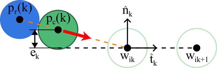
To measure tracking accuracy, we define a local cross-track error (CTE) at step $k$ using the current waypoint $\mathbf{w}_{i_{k}}$ and the local unit tangent of the curve. Let

$$\hat{\mathbf{t}}_{k}\triangleq\frac{\mathbf{w}_{(i_{k}+1)\bmod N}-\mathbf{w}_{i_{k}}}{\|\mathbf{w}_{(i_{k}+1)\bmod N}-\mathbf{w}_{i_{k}}\|_{2}},\qquad\hat{\mathbf{n}}_{k}\triangleq\begin{bmatrix}-\hat{t}_{k,y}\\ \hat{t}_{k,x}\end{bmatrix}.$$ (3)

The signed CTE is then

$$e_{k}\triangleq\big(\mathbf{p}_{c}(k)-\mathbf{w}_{i_{k}}\big)^{\top}\hat{\mathbf{n}}_{k},$$ (4)

and we use $|e_{k}|$ as the absolute tracking error. As illustrated in Fig. 2, this CTE is computed with respect to the local waypoint segment.

Figure 2: Local cross-track error (CTE) definition at step $k$. A local unit tangent $\hat{\mathbf{t}}_{k}$ is computed from the segment $\mathbf{w}_{i_{k}}\!\rightarrow\!\mathbf{w}_{(i_{k}+1)\bmod N}$, and the corresponding unit normal is $\hat{\mathbf{n}}_{k}$. The signed CTE is $e_{k}$, whose magnitude $|e_{k}|$ is used as the tracking error and for large-error termination.

II-D Success and Failure Criteria

An episode terminates successfully when the cell completes the target number of waypoint advancements:

$$\texttt{success}\iff A_{k}\geq A_{\mathrm{target}}.$$ (5)

We additionally enforce two termination conditions for bounded evaluation: (i) a large-error failure if the CTE exceeds a threshold $e_{\max}$,

$$\texttt{failure}\iff|e_{k}|>e_{\max},$$ (6)

and (ii) a truncation if the episode length reaches a maximum step budget $K_{\max}$.

II-E Flow Disturbance Model

The background flow varies over time through a smooth random process that evolves a scalar centerline speed $u(t)$ within bounds $[u_{\min},u_{\max}]$. A target speed is perturbed by Gaussian noise and the current speed relaxes toward this target with time constant $\tau$, yielding a temporally correlated disturbance that induces nonstationary drift during pushing. Detailed implementation and motivation for this disturbance model are provided in Sec. IV.

TABLE I: Problem setup parameters for the trajectory-tracking task.

Parameter	Symbol	Value
Number of waypoints on curve	$N$	140
Waypoint reach radius	$r_{\mathrm{wp}}$	2 px
Max episode steps	$K_{\max}$	3000
Failure threshold (CTE)	$e_{\max}$	10 px
Shared speed envelope	$v_{\max}$	50 px/s
Flow speed bounds (centerline)	$[u_{\min},u_{\max}]$	$[-10.8,\,10.8]$ px/s
Flow relaxation time constant	$\tau$	1.2
Flow noise standard deviation	$\sigma$	2.0

III METHOD

We propose a hybrid controller that combines a nominal model-predictive controller (MPC) with a learned residual policy. The MPC provides structured, contact-aware pushing behavior, while the residual policy outputs bounded corrections to improve robustness under nonstationary flow and model mismatch. Crucially, the residual is contact-gated: it is activated only when the robot is in contact with the cell, which stabilizes learning and prevents erratic behaviors during the approach phase. Fig. 3 summarizes the computation pipeline.

Figure 3: Contact-gated residual RL on top of MPC. The nominal MPC produces a planar velocity $\mathbf{u}^{\mathrm{mpc}}_{k}$. In parallel, the residual policy $\pi_{\theta}$ maps the observation $\mathbf{o}_{k}$ to a bounded action $\mathbf{a}_{k}\in[-1,1]^{2}$, which is scaled to a residual velocity $\Delta\mathbf{u}_{k}$ and gated by the contact indicator $\mathbb{I}_{\mathrm{ct}}(k)$. The final command is composed as $\mathbf{u}_{k}=\mathbf{u}^{\mathrm{mpc}}_{k}+\tilde{\Delta\mathbf{u}}_{k}$ and clipped to a shared speed envelope $v_{\max}$ before being applied to the simulator.

III-A Nominal MPC Backend

We use the MPC controller provided by the MicroPush control stack as the nominal backend. At each step $k$, the controller receives the current state estimate and the active goal waypoint $\mathbf{g}_{k}$ and produces a nominal planar command

$$\mathbf{u}^{\mathrm{mpc}}_{k}\in\mathbb{R}^{2},$$ (7)

which represents the desired robot planar velocity in the workspace frame. The MPC incorporates a contact-aware reference strategy that biases the robot to maintain a favorable pushing configuration relative to the cell and the goal, improving stability during sustained contact.

III-B Residual Policy and Composition

Let $\pi_{\theta}(\cdot)$ denote a stochastic policy that maps the current observation $\mathbf{o}_{k}$ to a bounded 2D action

$$\mathbf{a}_{k}=\pi_{\theta}(\mathbf{o}_{k}),\qquad\mathbf{a}_{k}\in[-1,1]^{2}.$$ (8)

Residual velocity parameterization (2D)

The policy outputs a bounded action $\mathbf{a}_{k}$, which is mapped to a residual planar velocity correction with a shared magnitude limit:

$$\Delta\mathbf{u}_{k}=\alpha\,v_{\max}\,\mathbf{a}_{k},$$ (9)

where $\alpha\in(0,1)$ is a scalar fraction that caps the residual magnitude relative to the common speed envelope $v_{\max}$.

Contact-gated composition

Let $\mathbb{I}_{\mathrm{ct}}(k)\in\{0,1\}$ be a contact indicator. We gate the residual such that it is applied only when contact is present:

$$\tilde{\Delta\mathbf{u}}_{k}=\mathbb{I}_{\mathrm{ct}}(k)\,\Delta\mathbf{u}_{k},$$ (10)

and compose the commanded planar velocity as

$$\mathbf{u}_{k}=\mathbf{u}^{\mathrm{mpc}}_{k}+\tilde{\Delta\mathbf{u}}_{k}.$$ (11)

Finally, we clip $\mathbf{u}_{k}$ to the shared speed envelope before applying it to the simulator.

III-C Shared Actuation Interface and Speed Envelope

All methods (pure MPC, pure PID, and our hybrid method) output a planar command $\mathbf{u}_{k}\in\mathbb{R}^{2}$. To ensure fairness and prevent any method from gaining an advantage by applying larger actuation, we enforce a shared speed envelope by clipping the command norm:

$$\mathbf{u}_{k}\leftarrow\mathbf{u}_{k}\cdot\min\!\left(1,\frac{v_{\max}}{\|\mathbf{u}_{k}\|_{2}+\epsilon}\right),$$ (12)

where $v_{\max}$ matches the bound used by the nominal controller and $\epsilon$ is a small constant for numerical stability. After saturation, the bounded $\mathbf{u}_{k}$ is applied to the simulator through the same actuation interface for all methods, so performance differences reflect decision quality rather than stronger actuation.

III-D Stabilizing Effect of Contact Gating

The approach phase, in which the robot moves toward the cell, is sensitive to observation noise and flow-induced drift. Allowing the learned policy to act during approach can destabilize contact acquisition and increase failures by steering the robot into unfavorable configurations. By contrast, the nominal MPC is designed to establish and maintain pushing contact. Contact gating restricts learning to the contact-rich regime, enabling the policy to focus on correcting systematic errors, such as lateral drift under flow, while preserving the MPC’s reliable approach behavior. This separation improves training stability and yields robust closed-loop tracking under time-varying disturbances.

IV LEARNING SETUP

This section describes learning-facing design choices: the observation provided to the residual policy, the time-varying background flow disturbance used during training and evaluation, and the reward shaping used for stable SAC training.

IV-A Observation Design

The residual policy is trained to correct nominal MPC behavior under nonstationary disturbances. To make the learning problem well-conditioned, we structure the observation into three interpretable blocks: geometry, motion, and control context. Geometry encodes task-relevant relative positions, motion provides local dynamics cues, and control context exposes the nominal command and tracking signals so the policy can learn when and how to correct.

TABLE II: Observation blocks provided to the residual policy.

Block	Contents
Geometry	Relative vectors: robot-to-cell $(\mathbf{p}_{c}-\mathbf{p}_{r})$ and cell-to-goal $(\mathbf{g}_{k}-\mathbf{p}_{c})$
Motion	Robot/cell planar velocities $(\mathbf{v}_{r},\mathbf{v}_{c})$ and robot heading $(\cos\theta_{r},\sin\theta_{r})$
Control context	Nominal MPC command $\mathbf{u}^{\mathrm{mpc}}_{k}$, contact flag $\mathbb{I}_{\mathrm{ct}}(k)$, signed cross-track error $e_{k}$, and local curve tangent $\hat{\mathbf{t}}_{k}$

Formally, at step $k$ we define

$$\mathbf{r}^{rc}_{k} \triangleq\mathbf{p}_{c}(k)-\mathbf{p}_{r}(k)\in\mathbb{R}^{2},$$ (13)

$$\mathbf{r}^{cg}_{k} \triangleq\mathbf{g}_{k}-\mathbf{p}_{c}(k)\in\mathbb{R}^{2},$$ (14)

$$\mathbf{m}_{k} \triangleq\big[\mathbf{v}_{r}(k)^{\top},\ \mathbf{v}_{c}(k)^{\top},\ \cos\theta_{r}(k),\ \sin\theta_{r}(k)\big]^{\top}\in\mathbb{R}^{6},$$ (15)

where $\mathbf{g}_{k}$ is the active waypoint. The control-context signals include the nominal MPC command $\mathbf{u}^{\mathrm{mpc}}_{k}\in\mathbb{R}^{2}$, the binary contact indicator $\mathbb{I}_{\mathrm{ct}}(k)\in\{0,1\}$, the signed cross-track error $e_{k}$, and the local unit tangent $\hat{\mathbf{t}}_{k}\in\mathbb{R}^{2}$:

$$\mathbf{c}_{k}\triangleq\big[(\mathbf{u}^{\mathrm{mpc}}_{k})^{\top},\ \mathbb{I}_{\mathrm{ct}}(k),\ (\hat{\mathbf{t}}_{k})^{\top},\ e_{k}\big]^{\top}\in\mathbb{R}^{6}.$$ (16)

The final observation is the concatenation

$$\mathbf{o}_{k}\triangleq\big[(\mathbf{r}^{rc}_{k})^{\top},\ (\mathbf{r}^{cg}_{k})^{\top},\ \mathbf{m}_{k}^{\top},\ \mathbf{c}_{k}^{\top}\big]^{\top}\in\mathbb{R}^{16}.$$ (17)

Normalization

We first apply task-scale normalization inside the environment: position-like terms are divided by the workspace extent, velocity-like terms are divided by $v_{\max}$, and unit-vector terms are clipped to $[-1,1]$. During SAC training, we additionally apply running observation normalization to stabilize updates under varying flow conditions.

IV-B Time-Varying Flow Disturbance

To model background microfluidic drift, the simulator applies a laminar Poiseuille profile aligned with a fixed channel axis $\hat{\mathbf{d}}$ and varying only along the cross-channel coordinate $y$:

$$\mathbf{u}_{f}(\mathbf{x},k)=u_{k}\left(1-\left(\frac{y}{R}\right)^{2}\right)\hat{\mathbf{d}},$$ (18)

where $R$ is the channel half-width and $u_{k}$ is the centerline speed at step $k$. In practice, we modulate only the centerline speed $u_{k}$, while the spatial profile is handled internally by the simulator.

Figure 4: Poiseuille flow model used as a drift disturbance. The flow is aligned with a fixed channel axis $\hat{\mathbf{d}}$ and has a parabolic speed profile across the channel width $2R$. We randomize only the centerline speed $u_{k}$ over time.

To induce nonstationary disturbances, we evolve the centerline speed using a temporally correlated random process. Let $\tilde{u}_{k}$ denote a clipped noisy target speed and $u_{k}$ the realized centerline speed. With $\Delta t=1/f_{\mathrm{sim}}$ and $f_{\mathrm{sim}}=60$ Hz, we update

$$\tilde{u}_{k+1} =\mathrm{clip}\!\left(\tilde{u}_{k}+\sigma\sqrt{\Delta t}\,\epsilon_{k},\ u_{\min},\ u_{\max}\right),$$ (19)

$$\hfill\epsilon_{k}\sim\mathcal{N}(0,1),$$

$$u_{k+1} =\mathrm{clip}\!\left(u_{k}+\alpha\left(\tilde{u}_{k+1}-u_{k}\right),\ u_{\min},\ u_{\max}\right),$$ (20)

$$\hfill\alpha=1-\exp\!\left(-\frac{\Delta t}{\tau}\right).$$

where $\tau$ is the relaxation time constant and $\sigma$ controls disturbance intensity. Training and evaluation use the same flow bounds and correlation settings (Tab. I).

IV-C Reward Shaping

The residual policy is trained with a shaped reward that promotes steady advancement along the reference curve while penalizing tracking error and unnecessary corrections. At each step $k$, we use

$$r_{k} =w_{\mathrm{prog}}\,\Delta d_{k}+w_{\mathrm{wp}}\,\Delta n^{\mathrm{wp}}_{k}-w_{\mathrm{track}}\,|e_{k}|-w_{\mathrm{time}}$$

$$\quad-w_{\Delta u}\,\|\Delta\mathbf{u}_{k}\|_{2}^{2}-w_{\Delta u_{s}}\,\|\Delta\mathbf{u}_{k}-\Delta\mathbf{u}_{k-1}\|_{2}^{2}+r^{\mathrm{term}}_{k}.$$ (21)

Here, $\Delta n^{\mathrm{wp}}_{k}\in\mathbb{Z}_{\geq 0}$ is the number of waypoint advances at step $k$, and $e_{k}$ is the signed cross-track error. The local progress term is the reduction in distance to the active waypoint,

$$\Delta d_{k}\triangleq d^{\mathrm{wp}}_{k-1}-d^{\mathrm{wp}}_{k},\qquad d^{\mathrm{wp}}_{k}\triangleq\|\mathbf{p}_{c}(k)-\mathbf{w}_{i_{k}}\|_{2}.$$ (22)

We define the applied residual correction as the deviation between the executed planar command, after contact gating and any saturation, and the nominal MPC command,

$$\Delta\mathbf{u}_{k}\triangleq\mathbf{u}_{k}-\mathbf{u}^{\mathrm{mpc}}_{k},$$ (23)

which becomes zero when contact-gating disables the residual, and may be reduced when the shared speed envelope clips the composed command.

The terminal reward is

$$r^{\mathrm{term}}_{k}=\begin{cases}+r_{\mathrm{succ}},&\text{if success},\\ -r_{\mathrm{fail}},&\text{if failure (large CTE)},\\ 0,&\text{if truncated at }K_{\max}.\end{cases}$$ (24)

Interpretation

The progress and waypoint terms encourage consistent advancement; the tracking penalty limits lateral drift; the time penalty discourages dithering; and the residual magnitude and smoothness penalties regularize the learned correction to remain small and non-oscillatory. All coefficients are listed in Tab. III.

TABLE III: Reward terms and coefficients used in this work.

Term	Coefficient
Local progress	$w_{\mathrm{prog}}=5.0$
Waypoint advance	$w_{\mathrm{wp}}=3.0$
Cross-track penalty	$w_{\mathrm{track}}=0.12$
Time penalty	$w_{\mathrm{time}}=0.002$
Residual magnitude penalty	$w_{\Delta u}=0.005$
Residual smoothness penalty	$w_{\Delta u_{s}}=0.002$
Success reward	$r_{\mathrm{succ}}=8.0$
Failure penalty	$r_{\mathrm{fail}}=2.0$

V EXPERIMENTS

We evaluate contact-gated residual RL on a contact-rich cell-pushing task with time-varying background flow. Our experiments address: (i) whether the residual policy improves robustness over nominal controllers under nonstationary disturbances, and (ii) whether the learned correction generalizes to unseen curve geometries when training is restricted to a single curve family.

V-A Training Protocol

Algorithm and implementation

We train the residual policy using Soft Actor-Critic (SAC) with an MLP actor–critic ($[256,256]$ hidden units) for $5\times 10^{5}$ environment steps. Observations are normalized in two stages: (i) task-scale normalization inside the environment, and (ii) running mean/variance normalization during training using a vectorized normalizer whose statistics are frozen and reused at evaluation. Reward normalization is enabled during training for stability and disabled during evaluation.

Training task distribution (clover curve)

Training uses a compact clover reference curve that repeatedly changes curvature and direction within a small workspace, creating frequent contact-rich interactions under flow. The curve is implemented as a composite of two orthogonal lemniscate segments. Let a base lemniscate be

$$\gamma_{0}(t)=\begin{bmatrix}a\sin t\\ b\sin t\cos t\end{bmatrix},\qquad t\in[0,2\pi),$$ (25)

and let $\mathcal{R}_{90}$ denote a $90^{\circ}$ rotation. The full clover trajectory is generated by concatenating $\gamma_{0}(t)$ and $\mathcal{R}_{90}\gamma_{0}(t)$ with consistent orientation, then sampling $N$ waypoints uniformly in the curve parameter to form $\{\mathbf{w}_{i}\}_{i=0}^{N-1}$. Fig. 5 shows a snapshot of the task and visualization conventions.

Figure 5: Training task snapshot (clover curve) under time-varying background flow. The cell (green) is pushed by the microrobot (blue) to follow the reference curve (orange). The current waypoint is shown with a marker and reach region. The cell and robot trajectories are overlaid to illustrate tracking behavior under drift.

During training, we randomize initial conditions and geometry to prevent overfitting: curve center jitter and curve scale parameters, randomized starting phase along the curve, and small pose jitter at reset. Background flow is always enabled and evolves according to Sec. IV-B, with centerline speed initialized uniformly in a bounded range and then updated by the temporally correlated process.

Hyperparameters

Tab. IV summarizes key SAC hyperparameters and evaluation settings used during training.

TABLE IV: SAC training hyperparameters and implementation settings.

Hyperparameter	Value
Total training steps	$5\times 10^{5}$
Policy / critic network	MLP, $[256,256]$
Learning rate	$3\times 10^{-4}$
Replay buffer size	$1\times 10^{5}$
Learning starts	$5\times 10^{3}$ steps
Batch size	256
Discount factor $\gamma$	0.99
Target smoothing $\tau$	0.005
Train frequency	1 step
Gradient steps per update	2
Observation normalization	running mean/variance (frozen at eval)
Reward normalization	train: on, eval: off
Evaluation during training	every 5k steps, 10 episodes

V-B Model Selection: Residual Bound Fraction $\alpha$

We select the residual bound fraction $\alpha$ in Eq. (9), which limits the maximum residual correction as $\|\Delta\mathbf{u}\|_{2}\leq\alpha v_{\max}$. We train three SAC policies for $5\times 10^{5}$ steps each with $\alpha\in\{0.05,\,0.15,\,0.30\}$ while keeping all other settings fixed. Fig. 6 reports evaluation mean return and success rate during training (raw traces with light lines and a smoothed curve for readability). Tab. V summarizes final performance.

Figure 6: Residual bound sweep for model selection. We train three policies with $\alpha\in\{0.05,0.15,0.30\}$ and report evaluation mean return (top) and success rate (bottom) during training. Light traces show raw evaluation values; dark traces show a smoothed curve.

TABLE V: Residual bound sweep results. $n=20$ episodes are evaluated for each $\alpha$. Completion time and CTE are computed over successful episodes only; progress ratio is computed over all episodes.

$\alpha$	$n$	Success	Time${}_{\text{succ}}$ (s)	CTE${}_{\text{succ}}$ (px)	Progress
0.05	20	0.10	19.87	0.951	0.299
0.15	20	1.00	19.36	0.737	1.000
0.30	20	0.85	21.56	0.698	0.920

A very small bound ($\alpha=0.05$) under-corrects flow-induced drift, leading to frequent failures and low progress. Increasing the bound to $\alpha=0.15$ yields the best overall performance, achieving high success with improved tracking. A larger bound ($\alpha=0.30$) remains competitive in tracking error but reduces reliability and efficiency, consistent with occasional over-correction under disturbance. Based on this sweep, we use $\alpha=0.15$ for all main comparisons against nominal baselines below.

V-C Evaluation Protocol

Train–test split and generalization

We train on the clover curve family (Fig. 5) and evaluate on three curve types: Circle, Clover (seen), and Square. During evaluation, we disable geometry randomization and initialization jitter, using fixed curve parameters and deterministic resets, to ensure reproducible comparisons across methods. Flow remains time-varying during evaluation under the same disturbance regime as training, with matched bounds, correlation time, and noise level.

Baselines and shared actuation envelope

We compare against two nominal controllers that share the same actuation interface and limits: (i) pure MPC, with the residual forced to zero while keeping the same control pipeline, and (ii) pure PID, evaluated under the same speed envelope. Improvements therefore reflect better decision-making under identical actuation constraints.

Metrics

We report four metrics per curve over multiple random seeds:

• Success rate: fraction of episodes that complete one lap.

• Completion time: time-to-success, computed over successful episodes only.

• Tracking error: mean absolute CTE, $\frac{1}{K}\sum_{k=1}^{K}|e_{k}|$.

• Progress ratio: waypoint advancement at termination normalized by the one-lap target, $\frac{A_{K}}{A_{\mathrm{target}}}$, computed over all episodes.

Implementation details

For the learned method, we load the observation-normalization statistics saved during training and disable further updates during evaluation. All controllers are evaluated under identical environment settings, including flow bounds, $\tau$, $\sigma$, waypoint resolution, and termination thresholds.

VI RESULTS AND DISCUSSION

We report quantitative comparisons across Circle, Clover (train), and Square under time-varying flow, and complement them with qualitative trajectory and failure analyses. Our goal is to validate that contact-gated residual RL improves robustness and tracking accuracy while operating under the same actuation envelope as nominal controllers. ResRL+MPC denotes the hybrid method with $\alpha=0.15$ selected in Sec. V-B.

VI-A Quantitative Results

Fig. 7 summarizes performance across 20 seeds using success rate, completion time, tracking error, and progress ratio. Overall, ResRL+MPC achieves higher success and lower tracking error than pure MPC and PID, with the largest gains on the more challenging curves. For successful trials, ResRL+MPC typically matches or improves completion time while reducing CTE, indicating more efficient disturbance rejection during sustained contact.

Progress ratio provides additional resolution beyond binary success. Pure MPC/PID often terminate early on Clover and Square, resulting in low progress ratios. In contrast, ResRL+MPC maintains higher progress even in unsuccessful trials, suggesting more consistent advancement before termination.

Figure 7: Quantitative results under time-varying flow for Circle (top), Clover (middle, train), and Square (bottom), aggregated over 20 seeds. We compare ResRL+MPC (with $\alpha=0.15$) against pure MPC and pure PID using success rate, completion time, tracking error (CTE), and progress ratio. Completion time and tracking error are computed over successful episodes only; progress ratio is computed over all episodes.

VI-B Qualitative Analysis and Failure Modes

Fig. 8 shows representative rollouts for each curve, including trajectories, tracking error over time, realized time-varying flow, and cell speed. See the accompanying supplementary video for the corresponding simulated rollouts. Two recurring patterns explain the quantitative gains.

Error spikes under disturbance changes

Baseline failures correlate with sharp spikes in tracking error that exceed the failure threshold. These spikes often coincide with rapid changes in flow magnitude or direction or with high-curvature segments where maintaining a stable pushing configuration is difficult. ResRL+MPC suppresses these spikes, keeping the error below threshold and enabling completion.

Disturbance rejection without stronger actuation

Despite identical speed limits, ResRL+MPC tracks the reference more faithfully when flow induces lateral drift. This indicates the residual primarily performs directional correction during contact rather than increasing actuation magnitude. The smoother speed profiles are consistent with the residual magnitude and smoothness penalties in the reward.

Figure 8: Qualitative rollouts under time-varying flow for Circle (left), Clover (middle, train), and Square (right). Top row: reference curve (dashed) and executed trajectories; insets show tracking error distributions. Middle rows: tracking error over time and realized flow speed. Bottom row: cell speed over time. Baseline failures correlate with sharp error spikes; ResRL+MPC suppresses spikes and maintains progress under disturbance.

VII CONCLUSIONS

We studied contact-rich cell pushing with a magnetic rolling microrobot under time-varying microfluidic flow, formulated as waypoint-based tracking of a planar reference curve. We proposed ResRL+MPC, which augments a contact-aware MPC backend with a contact-gated residual policy that outputs bounded 2D velocity corrections. Using a shared actuation interface and speed envelope, performance gains reflect improved decision-making rather than stronger actuation.

Across Circle, Clover, and Square trajectories under the same nonstationary disturbance process, ResRL+MPC improves success rate, progress ratio, and tracking accuracy relative to pure MPC and PID. A residual-bound sweep further shows that an intermediate correction limit yields the best authority–stability trade-off.

Future work will deploy the framework on a physical magnetic actuation system and validate it in microfluidic chips with live imaging.

VIII ACKNOWLEDGMENTS

The authors acknowledge the use of ChatGPT (OpenAI) to assist with English-language editing and clarity improvements in the manuscript, and to support code drafting and refactoring as well as the data plotting scripts used to generate figures. All technical content, experimental design, results, and conclusions were produced and verified by the authors.

References

- [1] (2006) Using inaccurate models in reinforcement learning. In Proceedings of the 23rd international conference on Machine learning, pp. 1–8. Cited by: §I.
- [2] (2019) End-to-end safe reinforcement learning through barrier functions for safety-critical continuous control tasks. In Proceedings of the AAAI conference on artificial intelligence, Vol. 33, pp. 3387–3395. Cited by: §I.
- [3] (2009) Two-dimensional contact and noncontact micromanipulation in liquid using an untethered mobile magnetic microrobot. IEEE Transactions on Robotics 25 (6), pp. 1332–1342. Cited by: §I.
- [4] (2018) Soft actor-critic: off-policy maximum entropy deep reinforcement learning with a stochastic actor. In International conference on machine learning, pp. 1861–1870. Cited by: §I.
- [5] (2014) Mobile microrobotic manipulator in microfluidics. Sensors and Actuators A: Physical 215, pp. 56–64. Cited by: §I.
- [6] (2000) Microrobots for micrometer-size objects in aqueous media: potential tools for single-cell manipulation. Science 288 (5475), pp. 2335–2338. Cited by: §I.
- [7] (2024) Efficient model learning and adaptive tracking control of magnetic micro-robots for non-contact manipulation. In 2024 IEEE International Conference on Robotics and Automation (ICRA), pp. 4534–4540. Cited by: §I.
- [8] (2022) Control and autonomy of microrobots: recent progress and perspective. Advanced Intelligent Systems 4 (5), pp. 2100279. Cited by: §I.
- [9] (2018) Residual reinforcement learning for robot control. arXiv preprint arXiv:1812.03201. Cited by: §I.
- [10] (2018) Development of a magnetic microrobot for carrying and delivering targeted cells. Science robotics 3 (19), pp. eaat8829. Cited by: §I.
- [11] (2011) Two-dimensional autonomous microparticle manipulation strategies for magnetic microrobots in fluidic environments. IEEE Transactions on Robotics 28 (2), pp. 467–477. Cited by: §I, §I.
- [12] (2013) Bio-inspired magnetic swimming microrobots for biomedical applications. Nanoscale 5 (4), pp. 1259–1272. Cited by: §I.
- [13] (2016) Model predictive control of a magnetically guided rolling microrobot. IEEE Robotics and Automation Letters 1 (1), pp. 455–460. Cited by: §I.
- [14] (2015) RodBot: a rolling microrobot for micromanipulation. In 2015 IEEE International Conference on Robotics and Automation (ICRA), pp. 4042–4047. Cited by: §I.
- [15] (2024) A reinforcement learning-based control strategy for robust interaction of robotic systems with uncertain environments. In 2024 IEEE International Conference on Robotics and Automation (ICRA), pp. 5788–5794. Cited by: §I.
- [16] (2021) Review on model predictive control: an engineering perspective. The international journal of advanced manufacturing technology 117 (5), pp. 1327–1349. Cited by: §I.
- [17] (2025) Autonomous vision-based magnetic microrobotic pushing of micro-objects and cells. arXiv preprint arXiv:2505.06450. Cited by: §I.
- [18] (2026) MicroPush: a simulator and benchmark for contact-rich cell pushing and assembly with a magnetic rolling microrobot. arXiv preprint arXiv:2602.23607. Cited by: §I.
- [19] (2023) Rolling helical microrobots for cell patterning. In 2023 International conference on manipulation, automation and robotics at small scales (MARSS), pp. 1–6. Cited by: §I.
- [20] (2025) Microrobot vascular parkour: analytic geometry-based path planning with real-time dynamic obstacle avoidance. arXiv preprint arXiv:2509.05500. Cited by: §I.
- [21] (2024) Quadrupole magnetic tweezers for precise cell transportation. IEEE Transactions on Biomedical Engineering 72 (4), pp. 1437–1444. Cited by: §I.
- [22] (2019) Robotic micromanipulation: fundamentals and applications. Annual Review of Control, Robotics, and Autonomous Systems 2 (1), pp. 181–203. Cited by: §I.