Accretion Disk Perturbations and Their Effects on Kerr Black Hole Superradiance and Gravitational Atom Evolution

Abstract

Kerr black hole (BH) superradiance can form gravitational atoms and produce characteristic gravitational-wave signals, providing a probe of ultralight bosons and dark matter. In realistic systems, accretion-disk gravity can shift energy levels and mix states, modifying the effective superradiant growth. We model the disk as a weak external perturbation via a multipole expansion and derive an effective three-level Hamiltonian for the $n=2$ subspace $\{\ket{211},\ket{210},\ket{21-1}\}$ in the weak-coupling regime. The leading disk effect is the quadrupolar ($\ell_{d}=2$) tidal field, whose symmetries fix the selection rules: axisymmetry gives only diagonal shifts, equatorial nonaxisymmetry activates $\Delta m=\pm 2$ mixing ($\ket{211}\leftrightarrow\ket{21-1}$), and breaking equatorial reflection opens $\Delta m=\pm 1$ couplings involving $\ket{210}$. As illustrations, a transient equatorial $m=2$ spiral wave drives the resulting two-level system and can suppress or quench superradiance by populating a decaying mode, while a quasi-static warp produces full three-level mixing and can generate narrow “growth gaps” near accidental near-degeneracies, with the same static reshuffling also allowing enhancement when weight shifts toward the growing mode. These findings demonstrate that accretion disk perturbations are a crucial environmental factor in determining the dynamics of BH superradiance and the evolution of boson clouds, thereby providing a more reliable theoretical basis for assessing the detectability of ultralight bosons in realistic astrophysical settings.

I Introduction

In recent years, ultralight bosons have attracted widespread attention as promising dark matter candidates, and Kerr black holes (BHs) provide a unique pathway to test such new physics. If a light scalar field exists around a rotating BH, then under the superradiance condition, incident waves can extract spin energy from the BH and become amplified Zouros and Eardley (1979). A fraction of the amplified waves may be trapped in the gravitational potential well, forming a macroscopically observable boson cloud. Together with the Kerr BH, this constitutes the so-called “gravitational atom” Baumann et al. (2019); Arvanitaki and Dubovsky (2010). This mechanism not only alters the spin evolution of BHs but may also generate characteristic gravitational wave signals, offering a core avenue to probe new particles in strong-gravity environments Brito et al. (2015); Arvanitaki et al. (2015).

However, in realistic astrophysical settings, the presence of accretion disks around BHs cannot be neglected. The mass distribution and geometry of accretion disks induce gravitational perturbations, which can significantly affect level couplings, effective growth rates, and even the occurrence of superradiance Arvanitaki and Dubovsky (2010). Existing studies have primarily focused on superradiance in isolated BH backgrounds, while systematic discussions of the dynamical evolution of gravitational atoms in the presence of accretion disks remain scarce. In particular, quantitative analyses of level coupling structures, growth-rate variations, and their impact on observability are still lacking.

Motivated by this, we study how thin-disk gravity perturbs the gravitational atom during the linear superradiant growth stage. We first justify a separation of timescales in which the superradiant growth of the dominant level is faster than the accretion-driven secular drift of the Kerr parameters, allowing $M$ and $\tilde{a}$ to be treated as effectively constant. We then model the disk solely through its Newtonian gravitational potential and develop a perturbative multipole expansion in the cloud region; in a freely falling frame the monopole shifts the energy zero and the dipole vanishes, so the leading physical effect is the quadrupolar ($\ell_{d}=2$) tidal field.

Focusing on the $n=2$ level subspace, we construct an effective three-level Hamiltonian in the basis $\{\ket{211},\ket{210},\ket{21-1}\}$ for $\alpha\equiv\mu M\ll 1$ and organize the dynamics by symmetry: the disk enters through source multipoles (projections onto $Y_{2m_{d}}$) and the selection rule $m_{d}=m^{\prime}-m$ fixes which sublevels couple, so axisymmetric disks give only diagonal shifts, equatorially symmetric but nonaxisymmetric structures activate the $\Delta m=\pm 2$ channel (mixing $\ket{211}\leftrightarrow\ket{21-1}$) while leaving $\ket{210}$ decoupled, and breaking equatorial-reflection symmetry opens $\Delta m=\pm 1$ couplings that involve $\ket{210}$ and yield full three-level mixing. We illustrate these channels with two representative configurations: a transient equatorial $m=2$ spiral density-wave packet (Gaussian envelope), which reduces to a driven two-level system and can suppress or even quench superradiance by inducing transitions into the decaying mode, and a quasi-static warped disk motivated by the Bardeen–Petterson scenario Bardeen and Petterson (1975); Papaloizou and Pringle (1983), whose static mixing can open narrow “growth gaps” when an accidental near-degeneracy reduces the effective splitting, with the resulting reshuffling either suppressing growth by admixing decaying components or enhancing it by shifting weight toward the growing mode.

The remainder of the paper is organized as follows. In Sec. II we review the gravitational-atom framework and introduce the effective multi-level description used in this work. In Sec. III we establish the timescale hierarchy, formulate the disk perturbation in a spherical-harmonic expansion, and derive the symmetry-based selection rules. In Sec. IV we present two representative disk models (equatorial spiral waves and static warps) and quantify their impact on level mixing and the effective growth rate. Sec. V is the conclusion and discussion. Technical details and auxiliary derivations are collected in the Appendices. Throughout this work, we use units $G=c=\hbar=1$.

II Gravitational Atoms and Multi-Level Systems

Consider a scalar field $\Phi$ of mass $\mu$ in Kerr spacetime, satisfying the Klein–Gordon equation

$$\left(g^{\mu\nu}\nabla_{\mu}\nabla_{\nu}-\mu^{2}\right)\Phi=0,$$ (1)

where the Kerr metric $g_{\mu\nu}$ in Boyer–Lindquist coordinates is given by

$$ds^{2}=-\left(1-\frac{2Mr}{\Sigma}\right)\ \mathrm{d}t^{2}-\frac{4Mar\sin^{2}\theta}{\Sigma}\ \mathrm{d}t\ \mathrm{d}\phi+\frac{\Sigma}{\Delta}\ \mathrm{d}r^{2}+\Sigma\ \mathrm{d}\theta^{2}+\left(r^{2}+a^{2}+\frac{2Ma^{2}r\sin^{2}\theta}{\Sigma}\right)\sin^{2}\theta\ \mathrm{d}\phi^{2}$$ (2)

with $\Sigma\equiv r^{2}+a^{2}\cos^{2}\theta$, $\Delta\equiv r^{2}-2Mr+a^{2}$ and the spin parameter $a\equiv J/M$. The event horizon radius is $r_{+}=M+\sqrt{M^{2}-a^{2}}$ and the BH angular velocity is $\Omega_{H}=\frac{a}{2Mr_{+}}$. The solutions of Eq. (1) can be separated as Brill et al. (1972)

$$\Phi(t,\bm{r})=\ \mathrm{e}^{-\mathrm{i}\omega t}\ \mathrm{e}^{\mathrm{i}m\phi}S_{\ell m}(\theta)R_{n\ell}(r),$$ (3)

Due to the presence of the BH horizon, the eigenvalue $\omega$ of Eq. (3) yields a complex eigenfrequency

$$\omega=\omega_{R}+\mathrm{i}\Gamma,$$ (4)

where the real part $\omega_{R}$ corresponds to the gravitational atom spectrum and the imaginary part $\Gamma$ denotes the superradiant growth rate. Here we define $\omega_{R}\equiv\omega_{n\ell m}$ and $\Gamma\equiv\Gamma_{n\ell m}$. Explicit expressions for these quantities are given by Detweiler (1980); Baumann et al. (2019)

$$\Gamma_{n\ell m}=\mu r_{+}C_{n\ell m}(m\Omega_{H}-\omega)\alpha^{4\ell+4},$$ (5)

$$\omega_{n\ell m}\simeq\mu\left(1-\frac{\alpha^{2}}{2n^{2}}-\frac{\alpha^{4}}{8n^{4}}+\frac{(2\ell-3n+1)\alpha^{4}}{n^{4}(\ell+1/2)}+\frac{2\tilde{a}m\alpha^{5}}{n^{3}\ell(\ell+1/2)(\ell+1)}\right),$$ (6)

with

$$C_{n\ell m} =\frac{2^{4\ell+1}(2\ell+n+1)!}{(\ell+n+1)^{2\ell+4}n!}\left[\frac{\ell!}{(2\ell)!(2\ell+1)!}\right]^{2}\times\prod_{j=1}^{\ell}\left[j^{2}\left(1-a^{2}/M^{2}\right)+r_{+}^{2}\left(m\Omega_{H}-\omega\right)^{2}\right],$$ (7)

in the weak-coupling limit $\alpha\equiv\mu M\ll 1$. Superradiance requires $\Gamma>0$, i.e. $m\Omega_{H}>\omega$. As the process proceeds, the occupation number of the growing state increases exponentially, and the boson cloud continuously extracts spin energy from the BH, reducing $\Omega_{H}$. When the system evolves to the critical condition $m\Omega_{H}\simeq\omega$, the growth rate $\Gamma\propto(m\Omega_{H}-\omega)$ vanishes, halting superradiance. At this stage, the boson cloud ceases to grow and the system reaches saturation, often referred to as the steady state of the gravitational atom, where the BH spin-down and boson cloud energy storage achieve dynamic equilibrium Yoshino and Kodama (2012).

Figure 1: Partial energy levels of the gravitational atom. The states $\ket{211}$, $\ket{210}$, and $\ket{21-1}$ are shown together with the nearby $\ket{200}$ level. Green solid lines denote growing states, red dashed lines denote decaying states. $\Delta E$ is the energy difference between $\ket{210}$ and $\ket{200}$, while $\epsilon_{h}$ denotes the splitting between adjacent magnetic quantum numbers $m$ within the $\ket{21m}$ subspace.

In this work, we restrict attention to three levels of the gravitational atom: $\ket{211}$, $\ket{210}$, and $\ket{21-1}$, treating the system as a three-level model and applying perturbation theory. To this end, we impose constraints on the strength of accretion-disk perturbations. From Eq. (6), the energy difference between $\ell=1$ and $\ell=0$ levels is

$$\Delta E\simeq\frac{1}{2}\alpha^{4},$$ (8)

while the splitting between adjacent $m$ states in the $\ket{21m}$ subspace is

$$\epsilon_{h}=\frac{1}{12}\tilde{a}\alpha^{5},$$ (9)

with the dimensionless spin parameter $\tilde{a}\equiv a/M$. Since $\epsilon_{h}\ll\Delta E$ in the small-$\alpha$ region, the three states $\{\ket{211},\ket{210},\ket{21-1}\}$ above can be regarded as a complete basis for describing the evolution of the gravitational atom. Here the $\ket{211}$ state is a growing mode, while $\ket{210}$ and $\ket{21-1}$ are decaying modes. In the complete basis $\{\ket{211},\ket{210},\ket{21-1}\}$, the background Hamiltonian matrix reads

$$H_{0}=\begin{pmatrix}E+\epsilon_{h}&0&0\\ 0&E&0\\ 0&0&E-\epsilon_{h}\end{pmatrix},$$ (10)

with the energy level

$$E\equiv\omega_{210}=-\mu\left(\frac{1}{8}\alpha^{2}+\frac{7}{128}\alpha^{4}\right),$$ (11)

accurate to the order $\mathcal{O}(\alpha^{4})$, since $\epsilon_{h}=\frac{1}{12}\tilde{a}\alpha^{5}$. Furthermore, if the off-diagonal elements of the accretion-disk perturbation Hamiltonian satisfy

$$|H_{21m,21m^{\prime}}|\ll\epsilon_{h},$$ (12)

the system can be treated by perturbation theory. Due to the perturbation of the accretion-disk, these three states undergo mixing

$$\ket{\psi_{c}}=c_{g}\ket{211}+c_{d}^{(1)}\ket{210}+c_{d}^{(2)}\ket{21-1},$$ (13)

and the effective growth rate of this state is (see Appendix A)

$$\Gamma_{\mathrm{eff}}=|c_{g}|^{2}\Gamma_{211}+|c_{d}^{(1)}|^{2}\Gamma_{210}+|c_{d}^{(2)}|^{2}\Gamma_{21-1}.$$ (14)

III Accretion Disks as Environmental Perturbations

III.1 Time scale Hierarchy and Negligible Accretion-Driven Evolution

Before modeling the disk gravity as an external perturbation, we first justify that the secular evolution of the Kerr parameters induced by accretion is negligible during the linear superradiant growth stage Arvanitaki and Dubovsky (2010). The physical question is simple: does accretion change the horizon angular velocity fast enough to noticeably move the system away from (or toward) the superradiant condition $m\Omega_{H}>\omega_{R}$ while the cloud is growing? This is answered by comparing two timescales,

$$\tau_{\mathrm{sr}}\equiv\Gamma_{211}^{-1},\qquad\tau_{\Omega}\equiv\frac{\Omega_{H}}{\left|\dot{\Omega}_{H}\right|}.$$ (15)

Here $\tau_{\mathrm{sr}}$ characterizes how rapidly the dominant level $\ket{211}$ amplifies, while $\tau_{\Omega}$ characterizes how rapidly accretion drifts $\Omega_{H}$. If $\tau_{\mathrm{sr}}\ll\tau_{\Omega}$, then $M$ and $\tilde{a}$ may be treated as constants over the growth epoch, and the disk can be regarded as an external perturbation acting on an effectively fixed Kerr background. In practice, we impose a conservative separation $\tau_{\mathrm{sr}}\leq\epsilon\,\tau_{\Omega}$ with $\epsilon\ll 1$.

We begin with $\tau_{\Omega}$, because it is set primarily by the time-averaged accretion strength. The Eddington luminosity $L_{\mathrm{Edd}}$ corresponds to the balance between gravity and radiation pressure on ionized gas (via Thomson scattering). Assuming a radiative efficiency $L=\eta\dot{M}$ Frank et al. (2002); Novikov and Thorne (1973), it defines the Eddington accretion rate

$$\dot{M}_{\mathrm{Edd}}\equiv\frac{L_{\mathrm{Edd}}}{\eta}.$$ (16)

It is then convenient to parametrize the long-term inflow as

$$\langle\dot{M}\rangle\simeq D\,f_{\mathrm{Edd}}\,\dot{M}_{\mathrm{Edd}},$$ (17)

where $f_{\mathrm{Edd}}\equiv L/L_{\mathrm{Edd}}$ measures the accretion strength relative to the Eddington limit and $D\leq 1$ accounts for the intermittency (duty cycle) Cackett et al. (2018); Shabala et al. (2008). Defining the Salpeter time

$$\tau_{S}\equiv\frac{M}{\dot{M}_{\mathrm{Edd}}}\simeq 4.5\times 10^{7}\,\mathrm{yr},$$ (18)

one has $M/\langle\dot{M}\rangle=\tau_{S}/(Df_{\mathrm{Edd}})$, so the accretion timescale is essentially controlled by the single combination $Df_{\mathrm{Edd}}$. Differentiating $\Omega_{H}(M,\tilde{a})$ and using $\dot{J}=l_{\mathrm{isco}}\dot{M}$, where $l_{\mathrm{isco}}$ is the specific angular momentum at the innermost stable circular orbit (ISCO) (see Appendix B).

$$\tau_{\Omega}\simeq g(\tilde{a})\,\frac{\tau_{S}}{Df_{\mathrm{Edd}}},\qquad g(\tilde{a})\equiv\left|\frac{\tilde{a}\sqrt{1-\tilde{a}^{2}}}{\tilde{l}_{\mathrm{isco}}-\tilde{a}\left(2-\sqrt{1-\tilde{a}^{2}}\right)}\right|,$$ (19)

where $g(\tilde{a})=\mathcal{O}(1)$ encodes the order-unity dependence on the spin and on the specific angular momentum at the ISCO.

We next estimate $\tau_{\mathrm{sr}}$ for the dominant $\ket{211}$ level. In the weak-coupling regime, Eq. (5) yields

$$\Gamma_{211}=\mu r_{+}\,C_{211}\,(\Omega_{H}-\omega_{R})\,\alpha^{8},\qquad\tau_{\mathrm{sr}}=\Gamma_{211}^{-1}.$$ (20)

Using $\mu=\alpha/M$ and defining the dimensionless detuning

$$\Omega_{H}-\omega_{R}\equiv\frac{\tilde{\Delta}(\alpha)}{M},\qquad\tilde{\Delta}(\alpha)\equiv M(\Omega_{H}-\omega_{R}),$$ (21)

one obtains the scaling form

$$\tau_{\mathrm{sr}}=\frac{M}{(r_{+}/M)\,C_{211}\,\tilde{\Delta}(\alpha)}\,\alpha^{-9},$$ (22)

up to slowly varying prefactors. A key point for quantitative estimates is that $(r_{+}/M)C_{211}$ is not generically order unity; for $\tilde{a}=\mathcal{O}(1)$ one typically finds $C_{211}\sim 10^{-3}$, so replacing this prefactor by an $\mathcal{O}(1)$ constant can shift $\tau_{\mathrm{sr}}$ by orders of magnitude.

Combining Eqs. (19) and (22) with the conservative requirement $\tau_{\mathrm{sr}}\leq\epsilon\,\tau_{\Omega}$ yields an implicit lower bound on $\alpha$,

$$\alpha_{\min}\simeq\left[\frac{M\,Df_{\mathrm{Edd}}}{\epsilon\,g(\tilde{a})\,\tau_{S}}\cdot\frac{1}{(r_{+}/M)\,C_{211}\,\tilde{\Delta}(\alpha_{\min})}\right]^{1/9}$$ (23)

which makes the logic transparent: the worst case for neglecting accretion corresponds to the largest time-averaged inflow $Df_{\mathrm{Edd}}$ (shortest $\tau_{\Omega}$), while intermittent accretion ($D\ll 1$) only lengthens $\tau_{\Omega}$ and relaxes the bound as $\alpha_{\min}\propto(Df_{\mathrm{Edd}})^{1/9}$.

Finally, to obtain a concrete numerical estimate, we adopt a conservative benchmark with persistent accretion ($D\simeq 1$) and a sub-Eddington strength $f_{\mathrm{Edd}}=0.1$, representative of luminous but not near-Eddington disks (thereby avoiding strong dependence on radiative feedback while still maximizing secular drift). For a rapidly spinning stellar-mass Kerr BH with $M=10M_{\odot}$ and $\tilde{a}=0.9$, we impose the conservative separation $\tau_{\mathrm{sr}}\lesssim 0.01\,\tau_{\Omega}$. Using the scaling in Eq. (22) together with $\tau_{\Omega}\simeq g(\tilde{a})\tau_{S}/(Df_{\mathrm{Edd}})$, and adopting representative values $g(\tilde{a})=\mathcal{O}(1)$, $C_{211}\sim 10^{-3}$ and $\tilde{\Delta}(\alpha)\sim\mathcal{O}(0.1)$ in the regime of interest, we obtain a lower bound

$$\alpha\gtrsim 0.02,$$ (24)

for which the accretion-driven evolution of $M$ and $\tilde{a}$ is slow compared with the linear superradiant growth.

Physically, the lower bound arises because in the weak-coupling regime the superradiant rate is strongly suppressed at small $\alpha$ (for $\ell=1$, $\Gamma_{211}\sim\alpha^{9}$), reflecting the exponentially small near-horizon wave function amplitude when the cloud radius scales as $r_{c}\sim M/\alpha^{2}$. For sufficiently small $\alpha$, the growth becomes so slow that secular accretion-driven drift of $\Omega_{H}$ can no longer be neglected during the linear stage. We stress that this estimation is primarily controlled by the time-averaged inflow $Df_{\mathrm{Edd}}$ and scales as $\alpha_{\min}\propto(Df_{\mathrm{Edd}})^{1/9}$; for intermittent accretion ($D\ll 1$) the bound becomes correspondingly weaker. In the remainder of this work we therefore treat $M$ and $\tilde{a}$ as constants during the linear-growth stage and evaluate the level-dependent growth/decay rates $\Gamma$ using Eq. (5).

III.2 Spherical-Harmonic Expansion of the Disk Gravitational Perturbation

Under the strong gravity of the BH, captured matter drifts inward while transporting angular momentum outward, forming an accretion disk Shakura and Sunyaev (1973); Lynden-Bell and Pringle (1974); Pringle (1981). Only electrically neutral, non-magnetized disks are considered, so that the disk affects the gravitational atom solely through gravity. For simplicity, the disk is further assumed to be geometrically thin, lying on the equatorial plane or tilted by a small inclination angle. In this limit, the disk is described by a surface density $\Sigma(t,r,\phi)$ Frank et al. (2002).

Figure 2: Schematic configuration of the BH, the boson cloud, and a geometrically thin accretion disk. The cloud is characterized by a typical radius $r_{c}$, while the disk extends from the inner radius $r_{\rm in}$ to the outer radius $r_{\rm out}$. The hierarchy $r_{\rm in}<r_{c}<r_{\rm out}$ illustrates that the cloud typically resides well inside the bulk of the disk. For example, for $\tilde{a}=0.9$ and $\alpha=0.1$, one has $r_{\rm in}=r_{\rm isco}\approx 2.3M$, $r_{c}\simeq 400M$, and a representative outer radius $r_{\rm out}\sim 10^{5}M$.

III.2.1 Validity Domain for a Perturbative Multipole Treatment

We have shown above that, for $\alpha\gtrsim 0.02$ given by Eq. (24), the superradiant growth of the dominant $\ket{211}$ level is fast compared with the secular accretion-driven drift of the Kerr parameters, so that $M$ and $\tilde{a}$ may be treated as constants during the linear stage. We now impose the additional requirement needed to model the disk gravity as an external perturbation: in the cloud region, the disk potential should admit a rapidly convergent spherical-harmonic (multipole) expansion Thorne (1980) that is dominated by low $\ell$ Baumann et al. (2019). Since the addition theorem for $1/|\bm{r}-\bm{r}^{\prime}|$ converges differently depending on whether the field point lies inside or outside the source point, it is natural to split the disk at a radius $r_{0}\gtrsim r_{c}$ into an “inner” part ($r_{\rm in}<r^{\prime}<r_{0}$) and an “outer” part ($r_{0}<r^{\prime}<r_{\rm out}$). The perturbative description is quantitatively controlled provided

1. the cloud predominantly feels an outer tidal field (so that the outer-source expansion with convergence parameter $r/r^{\prime}<1$ is valid throughout the cloud support)

2. disk material within the cloud does not significantly back-react on the cloud profile.

We encode these requirements by two dimensionless control parameters,

$$\epsilon_{\Phi}(r_{0})\equiv\left|\frac{\Phi_{\mathrm{in}}(r_{c};r_{0})}{\Phi_{\mathrm{out}}(r_{c};r_{0})}\right|\ll 1,\qquad\epsilon_{M}(r_{c})\equiv\frac{M_{\rm in}(r_{c})}{M_{c}}\ll 1,$$ (25)

where $M_{\rm in}(r_{c})=2\pi\int_{r_{\rm in}}^{r_{c}}\Sigma(r^{\prime})\,r^{\prime}\,dr^{\prime}$ and, at the scaling level,

$$\Phi_{\mathrm{in}}(r_{c};r_{0})\sim\frac{2\pi}{r_{c}}\int_{r_{\mathrm{in}}}^{r_{0}}\Sigma(r^{\prime})\,r^{\prime}\,dr^{\prime},\qquad\Phi_{\mathrm{out}}(r_{c};r_{0})\sim 2\pi\int_{r_{0}}^{r_{\mathrm{out}}}\Sigma(r^{\prime})\,dr^{\prime},$$ (26)

with $r_{0}$ taken slightly above $r_{c}$ to guarantee rapid convergence in the cloud region.

To obtain an explicit $\alpha$-dependence, we adopt an axisymmetric equatorial power-law disk profile Shakura and Sunyaev (1973); Lynden-Bell and Pringle (1974),

$$\Sigma(r)=\Sigma_{0}\left(\frac{r}{M}\right)^{-p},$$ (27)

write $M_{c}=\mu_{c}M$, and choose $r_{0}\simeq r_{c}$. This gives

$$\epsilon_{\Phi}\sim\frac{1-p}{2-p}\,\frac{r_{c}^{2-p}-r_{\mathrm{in}}^{2-p}}{r_{c}\left(r_{\mathrm{out}}^{1-p}-r_{c}^{1-p}\right)},\qquad\epsilon_{M}=\frac{2\pi\Sigma_{0}M^{p-1}}{\mu_{c}(2-p)}\left(r_{c}^{2-p}-r_{\mathrm{in}}^{2-p}\right),$$ (28)

and for the $n=2$ cloud we take $r_{c}\simeq\frac{4}{\alpha^{2}}M$. Using representative thin-disk parameters $r_{\mathrm{in}}=6M$, $r_{\mathrm{out}}=10^{5}M$ Novikov and Thorne (1973); Frank et al. (2002), $p=3/4$, together with $\Sigma_{0}M\simeq 10^{-8}$ Shakura and Sunyaev (1973) and $\mu_{c}=10^{-2}$ Brito et al. (2015), one finds $\epsilon_{\Phi}(\alpha=0.1)\simeq 6.7\times 10^{-2}$, $\epsilon_{M}(\alpha=0.1)\simeq 8.9\times 10^{-3}$, while at $\alpha=0.03$ one has $\epsilon_{\Phi}\simeq 1.7\times 10^{-1}$ and $\epsilon_{M}\simeq 1.8\times 10^{-1}$. Requiring, for definiteness, $\epsilon_{\Phi},\epsilon_{M}\lesssim 0.2$ therefore yields the conservative estimate

$$\alpha\gtrsim 0.03,$$ (29)

up to ${\cal O}(1)$ uncertainties from the scaling estimate in Eq. (26) and the chosen tolerance. Since this lower bound is consistent with the timescale requirement at the order-of-magnitude level and both controls degrade as $\alpha$ decreases, we adopt the more conservative choice and define the working domain as

$$\alpha\gtrsim\max\!\left[0.02\ \text{(from timescales)},\ 0.03\ \text{(from disk multipoles)}\right]\simeq 0.03,$$ (30)

within which the disk self-gravity can be treated as a weak, external, low-multipole perturbation acting on the hydrogenic cloud basis.

III.2.2 Quadrupolar Perturbation

Since the disk material is nonrelativistic and weak-field, its gravitational field can be described by the Newtonian potential in a freely falling frame centered on the BH–cloud center of mass,

$$U(t,\bm{r})=-\int\frac{\rho(t,\bm{r}^{\prime})}{|\bm{r}-\bm{r}^{\prime}|}\,\mathrm{d}V^{\prime},$$ (31)

where $\rho(t,\bm{r}^{\prime})$ is the mass volume density. The spherical-harmonic addition theorem,

$$\frac{1}{|\bm{r}-\bm{r}^{\prime}|}=\sum_{\ell=0}^{\infty}\sum_{m=-\ell}^{\ell}\frac{4\pi}{2\ell+1}\,\frac{r^{\ell}}{{r^{\prime}}^{\ell+1}}\,Y_{\ell m}(\theta,\phi)\,Y_{\ell m}^{\ast}(\theta^{\prime},\phi^{\prime}),$$ (32)

then yields a multipole expansion of Eq. (31). The perturbing potential energy experienced by the boson cloud is

$$V(t,\bm{r})=\mu U(t,\bm{r})=-\sum_{\ell_{d}=0}^{\infty}\sum_{m_{d}=-\ell_{d}}^{\ell_{d}}\int\frac{4\pi\mu\rho(t,\bm{r}^{\prime})}{2\ell_{d}+1}\,\frac{r^{\ell_{d}}}{{r^{\prime}}^{\ell_{d}+1}}\,Y_{\ell_{d}m_{d}}(\theta,\phi)\,Y_{\ell_{d}m_{d}}^{\ast}(\theta^{\prime},\phi^{\prime})\,\mathrm{d}V^{\prime}.$$ (33)

The monopole contribution shifts the energy zero, while the dipole term vanishes in the freely falling frame Misner et al. (1973). The lowest multipole producing a physical effect is therefore the quadrupole term $\ell_{d}=2$,

$$V_{2}(t,\bm{r})=-\frac{4\pi\mu}{5}\sum_{m_{d}=-2}^{2}\int\rho(t,\bm{r}^{\prime})\,\frac{r^{2}}{{r^{\prime}}^{3}}\,Y_{2m_{d}}(\theta,\phi)\,Y_{2m_{d}}^{\ast}(\theta^{\prime},\phi^{\prime})\,\mathrm{d}V^{\prime}.$$ (34)

In the unperturbed basis, the perturbation matrix is

$$H_{m,m^{\prime}}=\braket{21m|V_{2}|21m^{\prime}},$$ (35)

where the hydrogenic wavefunctions follow from Eq. (3),

$$\braket{\bm{r}|n\ell m}\simeq e^{i\varepsilon_{n}t}\,R_{n\ell}(r)\,Y_{\ell m}(\theta,\phi).$$ (36)

This perturbation couples different levels of the gravitational atom and induces level mixing.

III.2.3 Symmetry Considerations and Selection Rules

The disk–induced level mixing is fixed once the quadrupolar ($\ell_{d}=2$) part of the perturbing potential is projected onto the unperturbed $\{\ket{21m}\}$ subspace. Starting from the $\ell_{d}=2$ term of the spherical-harmonic addition theorem, the quadrupolar contribution to the potential energy can be organized into “source multipoles” by defining

$$I_{d}^{(m_{d})}(t)\equiv\int\frac{\rho(t,\bm{r}^{\prime})}{{r^{\prime}}^{3}}Y_{2m_{d}}^{\ast}(\theta^{\prime},\phi^{\prime})\,\mathrm{d}V^{\prime},$$ (37)

so that the perturbation experienced by the cloud takes the compact form

$$V_{2}(t,\bm{r})=-\frac{4\pi\mu}{5}\,r^{2}\sum_{m_{d}=-2}^{2}I_{d}^{(m_{d})}(t)\,Y_{2m_{d}}(\theta,\phi),$$ (38)

which makes explicit that all disk geometry and time dependence enter only through $I_{d}^{(m_{d})}(t)$. The perturbation matrix in the unperturbed basis is

$$H_{m,m^{\prime}}(t)\equiv\braket{21m|V_{2}(t,\bm{r})|21m^{\prime}}=\int d^{3}r\,\psi_{21m}^{\ast}(\bm{r})\,V_{2}(t,\bm{r})\,\psi_{21m^{\prime}}(\bm{r}),$$ (39)

with $\psi_{21m}(\bm{r})=e^{i\varepsilon_{2}t}R_{21}(r)Y_{1m}(\theta,\phi)$ and inserting Eq. (38) yields a fully factorized expression,

$$H_{m,m^{\prime}}(t)=-\frac{4\pi\mu}{5}\sum_{m_{d}=-2}^{2}I_{d}^{(m_{d})}(t)\,\Bigl[\int_{0}^{\infty}dr\,r^{4}R_{21}^{2}(r)\Bigr]\,\Bigl[\int d\Omega\,Y_{2m_{d}}(\Omega)\,Y_{1m}(\Omega)\,Y_{1m^{\prime}}^{\ast}(\Omega)\Bigr].$$ (40)

The first bracket in Eq. (40) is purely radial. For the hydrogenic $2p$ wavefunction one finds

$$\int_{0}^{\infty}dr\,r^{4}R_{21}^{2}(r)=30a^{2},\qquad a\equiv(\mu\alpha)^{-1}=\frac{M}{\alpha^{2}},$$ (41)

so that $\mu a^{2}=M/\alpha^{3}$. The second bracket is the angular integral

$$I_{\Omega}(m,m^{\prime};m_{d})\equiv\int d\Omega\,Y_{2m_{d}}(\Omega)\,Y_{1m}(\Omega)\,Y_{1m^{\prime}}^{\ast}(\Omega),$$ (42)

which enforces the usual azimuthal selection rule. Using $Y_{\ell m}(\theta,\phi)\propto e^{im\phi}$, the $\phi$ integral implies that the integrand is nonzero only when the net phase is $\phi$-independent, i.e.

$$m_{d}+m-m^{\prime}=0\qquad\Longrightarrow\qquad m_{d}=m^{\prime}-m.$$ (43)

Therefore only the disk multipole with $m_{d}=m^{\prime}-m$ can contribute to the matrix element $H_{m,m^{\prime}}$. Substituting the radial result and the definition Eq. (42) back into Eq. (40) gives

$$H_{m,m^{\prime}}(t)=-\frac{24\pi M}{\alpha^{3}}\sum_{m_{d}=-2}^{2}I_{d}^{(m_{d})}(t)\,I_{\Omega}(m,m^{\prime};m_{d}),$$ (44)

which makes the logic transparent: the disk determines which $m_{d}$ channels are present via $I_{d}^{(m_{d})}(t)$, while angular-momentum addition fixes which $\ket{21m}$ sublevels can mix through Eq. (43).

Consequently, the symmetries of the disk determine which $m_{d}$ channels are present, and Eq. (43) then specifies which $\ket{21m}$ sublevels can mix. The key point is that $I_{d}^{(m_{d})}$ is just the projection of the disk density onto the quadrupolar spherical harmonic $Y_{2m_{d}}$,

$$I_{d}^{(m_{d})}(t)=\int\frac{\rho(t,\bm{r}^{\prime})}{r^{\prime 3}}\,Y_{2m_{d}}^{\ast}(\theta^{\prime},\phi^{\prime})\,dV^{\prime}.$$ (45)

Therefore any symmetry that makes the disk “orthogonal” to a given $Y_{2m_{d}}$ forces that coefficient to vanish. If the disk is axisymmetric ($\rho$ independent of $\phi^{\prime}$) Shakura and Sunyaev (1973); Lynden-Bell and Pringle (1974), then only the $m_{d}=0$ Fourier harmonic exists and all $m_{d}\neq 0$ projections vanish:

$$I_{d}^{(m_{d}\neq 0)}=0.$$ (46)

If the disk breaks axial symmetry but remains mirror-symmetric about the equatorial plane Papaloizou and Lin (1995); Kato (1983), then the $\ell=2$ harmonics with $m_{d}=\pm 1$ are forbidden because they are odd across the midplane:

$$Y_{2,\pm 1}\ \propto\ \sin\theta^{\prime}\cos\theta^{\prime}\,e^{\pm i\phi^{\prime}}\quad\stackrel{{\scriptstyle\theta^{\prime}\to\pi-\theta^{\prime}}}{{\longrightarrow}}\quad-\,Y_{2,\pm 1},$$ (47)

so the contributions from above and below the plane cancel in the integral and

$$I_{d}^{(\pm 1)}=0\qquad(\text{mirror-symmetric disk}).$$ (48)

By contrast $Y_{2,0}$ and $Y_{2,\pm 2}$ are even across the midplane, so $m_{d}=0,\pm 2$ are allowed whenever the disk has the corresponding azimuthal structure. In short: azimuthal symmetry kills $m_{d}\neq 0$, and mirror-symmetric reflection kills the “odd” $m_{d}=\pm 1$ quadrupole; getting $m_{d}=\pm 1$ requires breaking equatorial reflection.

For the $\{\ket{211},\ket{210},\ket{21-1}\}$ subspace, three cases are particularly relevant:

• Axisymmetric disk ($\partial_{\phi^{\prime}}\Sigma=0$): the $\phi^{\prime}$ integral in Eq. (45) vanishes unless $m_{d}=0$, and Eq. (43) forces $m=m^{\prime}$. The perturbation is therefore purely diagonal and induces no level mixing.

• Equatorial but nonaxisymmetric perturbations: $m_{d}=\pm 2$ components are generated, opening the $\Delta m=\pm 2$ channel that mixes $\ket{211}\leftrightarrow\ket{21-1}$. If the mass distribution remains symmetric under reflection about the equatorial plane, $V_{2}$ is even parity and matrix elements connecting the odd-parity state $\ket{210}$ to the even-parity states $\ket{211}$ and $\ket{21-1}$ vanish, so the dynamics reduces to an effective two-level system.

• Out-of-equatorial geometry Bardeen and Petterson (1975); Kumar and Pringle (1985): breaking equatorial-reflection symmetry allows $m_{d}=\pm 1$ components already at $\ell_{d}=2$, opening the $\Delta m=\pm 1$ channel and enabling couplings $\ket{211}\leftrightarrow\ket{210}$ and $\ket{210}\leftrightarrow\ket{21-1}$. In this case all three $m$-sublevels can mix.

From an effective-theory viewpoint, it is thus natural to classify disk perturbations by the symmetries they break—axial symmetry controls whether $m_{d}\neq 0$ channels exist, while equatorial-reflection symmetry controls whether the odd-parity $\ket{210}$ state can participate. Explicit time dependence affects resonance and secular accumulation, but does not modify the selection rule in Eq. (43).

IV Representative Accretion-Disk Models

As discussed in Sec. III.2.3 (see also Eq. (38)), the disk enters the quadrupolar perturbation through the source multipoles $I_{d}^{(m_{d})}(t)$, while the selection rule $m_{d}=m^{\prime}-m$ fixes which $\ket{21m}$ sublevels can be coupled. From this perspective, the relevant “environmental channels” are most transparently organized by the symmetries they break: breaking axial symmetry activates $m_{d}\neq 0$ components, whereas breaking equatorial-reflection symmetry permits the $m_{d}=\pm 1$ channel and allows the odd-parity state $\ket{210}$ to participate in the mixing. In contrast, whether a perturbation is explicitly time dependent primarily controls resonance and secular accumulation, but does not alter the underlying selection rule.

In the $\{\ket{211},\ket{210},\ket{21-1}\}$ basis, the leading disk-induced Hamiltonian can be viewed as a sum of symmetry-tagged contributions,

$$H(t)=H_{0}+H_{\mathrm{diag}}(\tilde{\Sigma}_{0})+H_{\mathrm{spiral}}(t;\tilde{\Sigma}_{2})+H_{\mathrm{warp}}(\tilde{\Sigma}),$$ (49)

where $H_{\mathrm{diag}}$ denotes the axisymmetric ($m_{d}=0$) level shifts, $H_{\mathrm{spiral}}$ represents the nonaxisymmetric but equatorially symmetric component that dominantly opens the $m_{d}=\pm 2$ channel ($\ket{211}\leftrightarrow\ket{21-1}$), and $H_{\mathrm{warp}}$ captures out-of-equatorial distortions that open the $m_{d}=\pm 1$ channel and mix $\ket{210}$ with the even-parity states. Since the disk potential is treated as a weak perturbation, these contributions add linearly at leading order.

Motivated by this symmetry-based organization, two representative disk configurations are considered in what follows. The first breaks axial symmetry while preserving equatorial-reflection symmetry (a time-dependent equatorial spiral perturbation), thereby inducing mixing within the even-parity subspace. The second preserves axial symmetry but breaks equatorial-reflection symmetry through a small tilt/warp, generating (quasi-)static couplings that can involve all three $m$-sublevels. The key features are summarized in Table 1.

Table 1: Representative disk-perturbation models and their symmetry properties in the quadrupolar ($\ell_{d}=2$) potential.

Model	Mass distribution	Geometry	Time dependence
Equatorial Gaussian spiral wave	Nonaxisymmetric	Equatorially symmetric	Yes
Static warped disk	Axisymmetric	Equatorially asymmetric	No

IV.1 Equatorial Spiral Density Wave with a Gaussian Envelope

IV.1.1 Equatorial Disk Oscillations

Guided by the symmetry considerations summarized above, we first consider perturbations that break axial symmetry while preserving equatorial-reflection symmetry. A geometrically thin equatorial disk can support several oscillation modes when externally perturbed, including eccentric modes Kato (1983); Lubow (1991) and spiral density waves Lin and Shu (1987); Goldreich and Tremaine (1979). The eccentric mode corresponds to azimuthal number $m=1$, while spiral waves may occur for a range of $m$. Since we restrict to the quadrupolar ($\ell_{d}=2$) gravitational perturbation and the equatorial disk is reflection symmetric, the discussion in Appendix C (around Eq. (C7)) implies that odd-$m$ components do not contribute to the relevant matrix elements. We therefore focus on even-$m$ oscillations.

For a general oscillatory surface density, only Fourier components with $|m|\leq 2$ can couple to the $\ell_{d}=2$ potential. It suffices to expand the surface density up to second order,

$$\Sigma(t,r^{\prime},\phi^{\prime})=\sum_{|m|\leq 2}\Sigma_{m}(t,r^{\prime})\,e^{-im\phi^{\prime}},$$ (50)

where the $m=0$ term describes the axisymmetric background disk and $m\neq 0$ encode nonaxisymmetric perturbations. Reality of $\Sigma$ requires $\Sigma_{-m}=\Sigma_{m}^{\ast}$.

The relative importance of the disk’s secular evolution can be assessed by comparing the viscous timescale $\tau_{\nu}\sim R^{2}/\nu$with the local Keplerian timescale $\tau_{K}\sim 1/\Omega_{K}(R)$ Pringle (1981). Using $\nu\sim\alpha_{\nu}c_{s}H$ and the thin-disk scaling $H/R\sim c_{s}/v_{K}=c_{s}/(R\Omega_{K})$ Novikov and Thorne (1973), one finds

$$\frac{\tau_{\nu}}{\tau_{K}}\sim\frac{R^{2}\Omega_{K}}{\nu}=\frac{1}{\alpha_{\nu}}\left(\frac{R}{H}\right)^{2}\gg 1.$$ (51)

Thus the axisymmetric background may be treated as time independent over the dynamical time of interest,

$$\Sigma(t,r^{\prime},\phi^{\prime})=\Sigma_{0}(r^{\prime})+\sum_{0<|m|\leq 2}\Sigma_{m}(t,r^{\prime})\,e^{-im\phi^{\prime}}.$$ (52)

With Eqs. (52) and (44), the leading perturbation Hamiltonian in the $\{\ket{211},\ket{210},\ket{21-1}\}$ basis takes the form

$$H_{\mathrm{diag}}(\tilde{\Sigma}_{0}) =\kappa\begin{pmatrix}-3\tilde{\Sigma}_{0}&0&0\\ 0&6\tilde{\Sigma}_{0}&0\\ 0&0&-3\tilde{\Sigma}_{0}\end{pmatrix},\quad H_{\mathrm{spiral}}(t;\tilde{\Sigma}_{2})=\kappa\begin{pmatrix}0&0&9\tilde{\Sigma}_{2}(t)\\ 0&0&0\\ 9\tilde{\Sigma}_{2}^{\ast}(t)&0&0\end{pmatrix}.$$ (53)

where $\kappa=2\pi\,\frac{M}{\alpha^{3}}$ and

$$\tilde{\Sigma}_{0}=\int_{r_{\mathrm{in}}}^{r_{\mathrm{out}}}\frac{\Sigma_{0}(r^{\prime})}{{r^{\prime}}^{2}}\,\mathrm{d}r^{\prime},\qquad\tilde{\Sigma}_{m}(t)=\int_{r_{\mathrm{in}}}^{r_{\mathrm{out}}}\frac{\Sigma_{m}(t,r^{\prime})}{{r^{\prime}}^{2}}\,\mathrm{d}r^{\prime}.$$ (54)

As anticipated from the symmetry discussion, the odd-parity state $\ket{210}$ decouples from $\ket{211}$ and $\ket{21-1}$ for an equatorially symmetric quadrupole perturbation. The problem therefore reduces to an effective two-level system, which we write as a sum of a time-independent part and a time-dependent interaction,

$$\begin{aligned} &H=H_{0}+H_{\mathrm{diag}}(\tilde{\Sigma}_{0})+H_{\mathrm{spiral}},\\ &H_{0}+H_{\mathrm{diag}}(\tilde{\Sigma}_{0})=\begin{pmatrix}E+\epsilon_{h}-3\kappa\tilde{\Sigma}_{0}&0\\ 0&E-\epsilon_{h}-3\kappa\tilde{\Sigma}_{0}\end{pmatrix},\\ &H_{\mathrm{spiral}}(t)=\begin{pmatrix}0&9\kappa\tilde{\Sigma}_{2}(t)\\ 9\kappa\tilde{\Sigma}_{2}^{\ast}(t)&0\end{pmatrix}.\end{aligned}$$ (55)

The time evolution of the amplitudes follows from the Schrödinger equation in the interaction picture,

$$i\frac{\mathrm{d}}{\mathrm{d}t}\begin{pmatrix}c_{g}\\ c_{d}^{(2)}\end{pmatrix}=\begin{pmatrix}0&9\kappa\tilde{\Sigma}_{2}(t)\,e^{2i\epsilon_{h}t}\\ 9\kappa\tilde{\Sigma}_{2}^{\ast}(t)\,e^{-2i\epsilon_{h}t}&0\end{pmatrix}\begin{pmatrix}c_{g}\\ c_{d}^{(2)}\end{pmatrix}.$$ (56)

which determines the level mixing driven by the nonaxisymmetric $m=\pm 2$ disk component.

IV.1.2 Time-Dependent Perturbation and State Evolution

Figure 3: Surface-density profile of an $m=2$ spiral density wave with a Gaussian envelope. The $m=2$ mode produces two spiral arms, while the Gaussian envelope localizes the perturbation radially. The pattern corotates and the wave packet drifts outward.

A convenient phenomenological model for the leading nonaxisymmetric $\ell_{d}=2$ channel is a localized $m=2$ spiral density-wave packet riding on top of an axisymmetric background disk. Physically, this describes a two-armed overdensity pattern whose center drifts radially with a group velocity $v_{g}$, so the associated quadrupolar tidal field felt by the cloud turns on when the packet overlaps the inner disk and then decays as the packet moves outward Lin and Shu (1987); Kato (1983); Adams et al. (1989). We parametrize the surface density as Miranda and Rafikov (2019)

$$\Sigma(r,\phi,t)=\Sigma_{0}(r)+A\,\frac{r_{0}}{r}\,\exp\!\left[-\frac{(r-r_{0}-v_{g}t)^{2}}{2\sigma_{r}^{2}}\right]\cos\!\left[2\phi-\bigl(k_{r}(r-r_{0})-\omega_{d}t\bigr)\right],$$ (57)

where $\Sigma_{0}(r)$ is the time-independent axisymmetric background, while the second term is a wave packet centered at $R(t)=r_{0}+v_{g}t$ with radial width $\sigma_{r}$. The cosine encodes an $m=2$ spiral pattern with radial wavenumber $k_{r}$ and pattern frequency $\omega_{d}$, and $A$ sets the perturbation amplitude.

For definiteness we adopt representative inner-disk values (Table 2) chosen to be conservative in the sense of maximizing the cumulative driving: $r_{0}$ is taken at an ISCO-scale radius (where the disk is densest and the tidal field is strongest), $\sigma_{r}$ is a few-$M$ localized feature, and $v_{g}\ll 1$ ensures a long driving duration $t_{\rm drive}\sim\sigma_{r}/v_{g}$. The choices of $k_{r}$ and $\omega_{d}$ set the effective driving frequency seen by the cloud but do not change the symmetry channel ($m=2$) being activated.

Table 2: Representative parameters for the Gaussian-envelope $m=2$ spiral-density-wave packet in Eq. (57). Ward (1986); Lin and Papaloizou (1986); Binney and Tremaine (2011); Kato (2001)

Parameter	Physical meaning	Representative value
$r_{0}$	Initial packet-center radius	$6M$
$v_{g}$	Group velocity of the packet	$0.002$
$\sigma_{r}$	Characteristic radial width	$3M$
$k_{r}$	Radial wavenumber (spiral pitch)	$0.5/M$
$\omega_{d}$	Pattern (mode) frequency	$0.001/M$
$A$	Perturbation amplitude scale	$\sim\Sigma_{0}$

To connect this model to the quadrupolar Hamiltonian, we expand the perturbation in azimuthal harmonics. Writing the cosine in Eq. (57) as a sum of exponentials shows that the only nonzero nonaxisymmetric components are $m=\pm 2$, so the relevant Fourier coefficient can be taken as

$$\Sigma_{2}(t,r)\simeq\frac{A}{2}\,\frac{r_{0}}{r}\,\exp\!\left[-\frac{(r-R(t))^{2}}{2\sigma_{r}^{2}}\right]\exp\!\left[-i\bigl(k_{r}(r-r_{0})-\omega_{d}t\bigr)\right],\qquad R(t)\equiv r_{0}+v_{g}t,$$ (58)

with $\Sigma_{-2}=\Sigma_{2}^{\ast}$ for a real surface density. The disk enters the two-level problem through the weighted radial moment

$$\tilde{\Sigma}_{2}(t)\equiv\int_{r_{\mathrm{in}}}^{r_{\mathrm{out}}}\frac{\Sigma_{2}(t,r^{\prime})}{r^{\prime 2}}\,dr^{\prime}.$$ (59)

Because the packet is localized around $r^{\prime}\simeq R(t)$, slowly varying factors may be evaluated at $R(t)$, while the rapidly varying phase produces a Gaussian Fourier suppression Wong (2001). This yields the estimate

$$\tilde{\Sigma}_{2}(t)\simeq\sqrt{\frac{\pi}{2}}\,r_{0}\sigma_{r}A\,e^{-k_{r}^{2}\sigma_{r}^{2}/2}\,\frac{e^{-i\Omega_{d}t}}{R(t)^{3}},\qquad\Omega_{d}\equiv k_{r}v_{g}-\omega_{d},$$ (60)

where $\Omega_{d}$ is the effective driving frequency seen by the cloud: the term $k_{r}v_{g}$ comes from the radial drift of the packet center, while $\omega_{d}$ is the intrinsic pattern rotation. Eq. (60) makes the physical control parameters explicit: the driving strength scales with $A$ and the geometric tidal falloff $R(t)^{-3}$, the duration is set by $t_{\rm drive}\sim\sigma_{r}/v_{g}$, and fine radial structure is exponentially suppressed by $e^{-k_{r}^{2}\sigma_{r}^{2}/2}$.

Substituting Eq. (60) into the interaction-picture evolution Eq. (56), the off-diagonal driving term becomes

$$9\kappa\,\tilde{\Sigma}_{2}(t)\,e^{2i\epsilon_{h}t}\;\simeq\;9\kappa\,\tilde{A}\,\frac{e^{i\delta t}}{R(t)^{3}},\qquad R(t)\equiv r_{0}+v_{g}t,$$ (61)

where we have defined the effective driving detuning

$$\delta\;\equiv\;2\epsilon_{h}-\Omega_{d},\qquad\Omega_{d}\equiv k_{r}v_{g}-\omega_{d}.$$ (62)

Thus the driven two-level dynamics is controlled by a competition between the maximum mixing strength (set by the peak quadrupolar coupling near $t\simeq 0$) and the detuning $\delta$ (set by the intrinsic level splitting $2\epsilon_{h}$ relative to the disk’s pattern frequency $\Omega_{d}$). It is therefore natural to introduce the dimensionless control parameter Binney and Tremaine (2011); Lichtenberg and Lieberman (2013)

$$\Lambda\;\equiv\;\frac{\Omega_{\rm mix}(t\simeq 0)}{|\delta|}\;\simeq\;\frac{9\kappa|\tilde{A}|/r_{0}^{3}}{\left|2\epsilon_{h}-(k_{r}v_{g}-\omega_{d})\right|},$$ (63)

where $\Omega_{\rm mix}(t)\equiv 9\kappa|\tilde{A}|/R(t)^{3}$ is the instantaneous mixing rate induced by the $m=\pm 2$ disk component. In addition, because the envelope moves outward with speed $v_{g}$, the driving acts effectively only over a duration $t_{\rm drive}\sim\sigma_{r}/v_{g}$, so smaller $v_{g}$ corresponds to longer coherent forcing and hence larger cumulative mixing, even when the instantaneous perturbation is weak.

The impact on the scalar cloud is conveniently quantified by the late-time effective growth rate

$$\Gamma_{\rm eff}(t)=|c_{g}(t)|^{2}\Gamma_{211}+|c_{d}(t)|^{2}\Gamma_{21-1},$$ (64)

and by the growth-factor ratio

$$\chi\equiv\frac{\Gamma_{\rm eff}(\infty)}{\Gamma_{\rm eff}(0)}.$$ (65)

For the superradiant initial condition $c_{g}(0)=1$, $c_{d}(0)=0$ one has $\Gamma_{\rm eff}(0)=\Gamma_{211}$, and the late-time ratio can be written directly in terms of the transferred population $P_{d}\equiv|c_{d}(\infty)|^{2}$,

$$\chi=\frac{\Gamma_{211}(1-P_{d})+\Gamma_{21-1}P_{d}}{\Gamma_{211}}=1-\left(1-\frac{\Gamma_{21-1}}{\Gamma_{211}}\right)P_{d}.$$ (66)

Eq. (66) makes the physics transparent: disk driving does not modify the microscopic rates $\Gamma_{211}$ and $\Gamma_{21-1}$, but it can redistribute probability between the growing and decaying levels; once $P_{d}$ becomes ${\cal O}(1)$, the decaying component can dominate and quench superradiance ($\chi<0$).

In practice, the mixing strength $P_{d}$ is controlled by the single ratio $\Lambda$ (enhanced by a long driving time $t_{\rm drive}$). This motivates the following interpretation of the $(\alpha,\Sigma_{0})$ scan in Fig. 4:

• $\Lambda\ll 1$: weak, off-resonant driving $\Rightarrow P_{d}\ll 1$ and $\chi\simeq 1$ (negligible mixing).

• $\Lambda\sim 1$: comparable coupling and detuning $\Rightarrow P_{d}={\cal O}(0.1\text{--}1)$ and $0<\chi<1$ (suppressed growth).

• $\Lambda\gg 1$ (especially when $|\delta|\lesssim t_{\rm drive}^{-1}$): strong/near-resonant transfer $\Rightarrow P_{d}\to{\cal O}(1)$ and $\chi<0$ (quench region).

The parametric dependence is also clear from Eq. (63): $\alpha$ enters mainly through the intrinsic splitting $\epsilon_{h}(\alpha)$ and the prefactor $\kappa\propto M/\alpha^{3}$, while the disk strength enters through $|\tilde{A}|\propto A$ and the geometric tidal falloff $r_{0}^{-3}$; finally, the duration of coherent forcing scales as $t_{\rm drive}\sim\sigma_{r}/v_{g}$, making small $v_{g}$ particularly efficient at accumulating mixing.

(a) $\Gamma_{\mathrm{eff}}(\infty)$	(b) $\chi\equiv\Gamma_{\mathrm{eff}}(\infty)/\Gamma_{\mathrm{eff}}(0)$

Figure 4: Scan in the $(\alpha,\Sigma_{0})$ plane for an equatorial $m=2$ spiral perturbation with a Gaussian envelope. (a) Steady-state effective growth rate $\Gamma_{\mathrm{eff}}(\infty)$; (b) growth-factor ratio $\chi\equiv\Gamma_{\mathrm{eff}}(\infty)/\Gamma_{\mathrm{eff}}(0)$, where $\chi\simeq 1$ indicates negligible mixing, $0<\chi<1$ suppression, and $\chi<0$ quenching of superradiance. Crosses mark $(\alpha,\Sigma_{0})=(0.032,6\times 10^{-13})$ (red), $(0.038,4\times 10^{-13})$ (blue), and $(0.044,3\times 10^{-13})$ (green) (see Fig. 5).

The results are summarized in Fig. 4. Fig. 4(a) shows that $\Gamma_{\rm eff}(\infty)$ varies most sensitively with $\alpha$, as expected because $\alpha$ controls both the intrinsic level splitting $2\epsilon_{h}(\alpha)$ (and hence the detuning $\delta$ relative to the disk pattern frequency) and the overall mixing scale through $\kappa\propto M/\alpha^{3}$, whereas changing the disk normalization (e.g. $\Sigma_{0}$ or $A$) mainly rescales the coupling amplitude and shifts the boundaries between behaviors. This structure is made transparent in Fig. 4(b), which plots the growth-factor ratio $\chi\equiv\Gamma_{\rm eff}(\infty)/\Gamma_{\rm eff}(0)$, directly tracking the population transfer from the growing state $\ket{211}$ to the decaying partner $\ket{21-1}$ via Eq. (66). Three regimes emerge: negligible mixing ($\chi\simeq 1$), where the forcing is too weak and/or off-resonant over the finite driving time so $P_{d}\ll 1$; suppression ($0<\chi<1$), where $P_{d}=\mathcal{O}(0.1\text{--}1)$ reduces $\Gamma_{\rm eff}$ without shutting off superradiance; and quench ($\chi<0$), where the decaying component dominates at late times, which requires simultaneously an $\mathcal{O}(1)$ peak coupling and approximate phase coherence over the envelope duration $|\delta|\ \lesssim\ t_{\rm drive}^{-1},\ t_{\rm drive}\sim\frac{\sigma_{r}}{v_{g}}$.

The corresponding time-domain behavior is shown in Fig. 5. Points in the quench region exhibit an $\mathcal{O}(1)$ transfer to the decaying level, so $|c_{d}(t)|^{2}$ dominates at late times and $\Gamma_{\rm eff}$ becomes negative. By contrast, in the negligible region the transfer remains small and the system stays close to the unperturbed superradiant trajectory, while points in the suppression band interpolate between these limits. This time-domain evolution therefore provides a direct dynamical confirmation of the regime classification in Fig. 4(b).

Figure 5: Time evolution of the two-level probabilities for several representative $(\alpha,\Sigma_{0})$ choices (crosses in Fig. 4). Solid and dashed curves show $|c_{g}(t)|^{2}$ and $|c_{d}^{(2)}(t)|^{2}$, respectively.

IV.2 Static Warped Disk: Equatorial-Symmetry Breaking

IV.2.1 Geometry and the $\Delta m=\pm 1$ Coupling Channel

We next consider perturbations that preserve axial symmetry but break equatorial-reflection symmetry, so that the $m_{d}=\pm 1$ channel is activated and the odd-parity state $\ket{210}$ can mix with $\ket{211}$ and $\ket{21-1}$. A tilted disk is generic if the angular-momentum axis of the inflowing material is misaligned with the BH spin. In a Kerr spacetime, frame dragging tends to align the inner disk with the BH equatorial plane while the outer disk remains tilted, producing a warped transition region (the Bardeen–Petterson effect) Bardeen and Petterson (1975); Papaloizou and Pringle (1983). The local tilt is described by an inclination angle $\beta(r)$. In addition, Lense–Thirring precession causes rings at different radius to precess at different rates. The resulting differential precession exerts a twisting torque which, if too large, can even tear the disk Doğan et al. (2018); Nixon et al. (2012). When viscous stresses are able to counteract this torque, the twist saturates Ogilvie (1999); we parametrize the residual twist by a phase $\gamma(r)$. For our purposes, only the leading effect of the warp on the quadrupolar potential is retained.

Figure 6: Accretion-disk geometry and notation. Left: Geometric construction of a thin warped disk. Each ring at radius $r$ is obtained by tilting the corresponding equatorial ring by $\beta(r)$ and applying a twist $\gamma(r)$; the small-tilt limit $\beta\ll 1$ is assumed Papaloizou and Pringle (1983); Pringle (1992). Right: schematic warped configuration in which the inner disk tends to align with the BH equatorial plane while the outer disk remains tilted, producing a warped transition region.

IV.2.2 Quasi-Static Warp Approximation

An important simplification is that the warped configuration can be treated as effectively static on the timescales relevant for the cloud evolution. Physically, any coherent Lense–Thirring precession of a global warp is expected to be strongly damped by viscous dissipation, so that the disk relaxes to a quasi-steady geometry rather than maintaining a long-lived precessing mode. This statement can be quantified in the Papaloizou–Pringle rigid-disk approximation Papaloizou and Pringle (1983), where viscous communication across the disk is fast enough that the warp responds coherently and the damping time $\tau_{\mathrm{damp}}$ can be compared directly to the global precession period $T_{p}$ Lodato and Pringle (2007). Using Eq. (D8) in Appendix D, one finds

$$\frac{\tau_{\mathrm{damp}}}{T_{p}}\sim\frac{2\tilde{a}}{\alpha_{2}}\left(\frac{M}{r_{\mathrm{in}}}\right)^{3/2}\left(\frac{r_{\mathrm{out}}}{r_{\mathrm{in}}}\right)\left(\frac{r_{\mathrm{in}}}{H}\right)^{2}.$$ (67)

For representative parameters $\alpha=0.1$, $\tilde{a}=0.9$, $r_{\mathrm{in}}\sim 6M$, $r_{\mathrm{out}}\sim 10^{5}M$, and $H/r_{\mathrm{in}}\sim 10^{-2}$, together with $\alpha_{2}\simeq 1/(2\alpha)$ in this approximation, this estimate gives

$$\frac{\tau_{\mathrm{damp}}}{T_{p}}\approx 0.04\ll 1,$$ (68)

implying that any global precession decays within less than a cycle and the disk settles into a steady warp. In the language of the source multipoles $I_{d}^{(m_{d})}(t)$, this conclusion can be phrased more directly: a warped configuration corresponds to an ultra–low–frequency contribution, i.e. the $\omega\to 0$ limit of a slowly varying perturbation. Therefore, on the timescales relevant for the cloud’s linear-growth stage, the warp acts as a quasi-static background. One may schematically parametrize any residual relaxation as

$$\tilde{\Sigma}(t)\simeq\tilde{\Sigma}\,e^{-t/\tau_{\mathrm{damp}}},$$ (69)

but for the present purposes it is sufficient to treat $\tilde{\Sigma}$ as constant over the timescale of interest.

IV.2.3 Static Gravitational Perturbation

To isolate the warp-induced effect, we assume an axisymmetric and time-independent surface density, so that only the $m_{d}=0$ (diagonal) and $m_{d}=\pm 1,\pm 2$ (warp) source multipoles are present at $\ell_{d}=2$. Following the decomposition in Eq. (49), we write the Hamiltonian in the $\{\ket{211},\ket{210},\ket{21-1}\}$ basis as

$$H\;=\;H_{0}\;+\;H_{\mathrm{diag}}(\tilde{\Sigma}_{0})\;+\;H_{\mathrm{warp}}(\tilde{\Sigma}),$$ (70)

where the axisymmetric surface-density moment is

$$\tilde{\Sigma}_{0}=\int_{r_{\mathrm{in}}}^{r_{\mathrm{out}}}\frac{\Sigma(r^{\prime})}{{r^{\prime}}^{2}}\,\mathrm{d}r^{\prime},$$ (71)

and the warp geometry is encoded in the weighted moment

$$\tilde{\Sigma}=\int_{r_{\mathrm{in}}}^{r_{\mathrm{out}}}\frac{\Sigma(r^{\prime})}{{r^{\prime}}^{2}}\,\beta(r^{\prime})\,e^{-i\gamma(r^{\prime})}\,\mathrm{d}r^{\prime}.$$ (72)

Keeping only terms linear in the small tilt $\beta\ll 1$ (see Appendix E for details), the diagonal contribution (from the axisymmetric component $m_{d}=0$) takes the form

$$H_{0}+H_{\mathrm{diag}}(\tilde{\Sigma}_{0})=\begin{pmatrix}E+\epsilon_{h}-3\kappa\tilde{\Sigma}_{0}&0&0\\ 0&E+6\kappa\tilde{\Sigma}_{0}&0\\ 0&0&E-\epsilon_{h}-3\kappa\tilde{\Sigma}_{0}\end{pmatrix},$$ (73)

while the warp-induced (equatorially asymmetric) part is

$$H_{\mathrm{warp}}(\tilde{\Sigma})=\frac{9\sqrt{2}}{2}\kappa\begin{pmatrix}0&-\tilde{\Sigma}&0\\ -\tilde{\Sigma}^{\ast}&0&\tilde{\Sigma}\\ 0&\tilde{\Sigma}^{\ast}&0\end{pmatrix}.$$ (74)

Notably, for a thin ring with a small local tilt $\beta(r^{\prime})\ll 1$ (Appendix E), one finds the warp amplitude in the linear order,

$$I_{d}^{(0)}={\cal O}(1),\qquad I_{d}^{(\pm 1)}={\cal O}(\beta)\,e^{\mp i\gamma},\qquad I_{d}^{(\pm 2)}={\cal O}(\beta^{2}),$$ (75)

so a small warp activates the $m_{d}=\pm 1$ channel already at $\ell_{d}=2$, whereas the $m_{d}=\pm 2$ channel is subleading in the linear-tilt approximation.

Figure 7: Effective growth rate $\Gamma_{\mathrm{eff}}$ as a function of the gravitational fine-structure constant $\alpha$ in the presence of a static warped-disk perturbation. Colors label the unperturbed initial-state compositions $(c_{g},c_{d}^{(1)},c_{d}^{(2)})=(1,0,0)$ (blue), $(1/\sqrt{2},\,1/\sqrt{2},\,0)$ (purple), $(4/\sqrt{17},\,0,\,1/\sqrt{17})$ (green), and $(2/\sqrt{6},\,1/\sqrt{6},\,1/\sqrt{6})$ (red). Solid curves show the unperturbed results, while dashed curves include the warp-induced mixing. The inset zooms into the small-$\alpha$ region. The vertical dashed line marks $\Delta_{\rm res}(\alpha)=0$ with $\Delta_{\rm res}\equiv\epsilon_{h}-9\kappa\tilde{\Sigma}_{0}$, where the diagonal splitting between $\ket{211}$ and $\ket{210}$ is suppressed and the static mixing is maximized.

Because the warped-disk perturbation is (quasi-)time independent, it does not provide a coherent drive as in the spiral case; instead it acts as a static basis rotation. The Hamiltonian is constant, so the cloud reorganizes into new stationary eigen-combinations that are mixtures of the unperturbed $\{\ket{211},\ket{210},\ket{21-1}\}$ sublevels. The microscopic growth/decay rates $\Gamma_{21m}$ are unchanged; any change in the effective growth rate therefore comes only from a reshuffling of probability among the three sublevels. In stationary perturbation theory this reshuffling is controlled by the ratio of the off-diagonal warp coupling $\bar{\Sigma}\equiv\frac{9\sqrt{2}}{2}\kappa\tilde{\Sigma}$ to the relevant diagonal splittings of $H_{0}+H_{\rm diag}$, namely the $m=+1\leftrightarrow 0$ and $0\leftrightarrow-1$ gaps

$$\begin{aligned} \Delta_{g0}\equiv(E+\epsilon_{h}-3\kappa\tilde{\Sigma}_{0})-(E+6\kappa\tilde{\Sigma}_{0})=\epsilon_{h}-9\kappa\tilde{\Sigma}_{0},\\ \Delta_{0d}\equiv(E+6\kappa\tilde{\Sigma}_{0})-(E-\epsilon_{h}-3\kappa\tilde{\Sigma}_{0})=\epsilon_{h}+9\kappa\tilde{\Sigma}_{0}.\end{aligned}$$ (76)

To leading order, the perturbed cloud state can be written as

$$\ket{\psi_{c}}=\left(c_{g}+\frac{\bar{\Sigma}}{\Delta_{g0}}c_{d}^{(1)}\right)\ket{211}+\left(c_{d}^{(1)}-\frac{\bar{\Sigma}^{\ast}}{\Delta_{g0}}c_{g}-\frac{\bar{\Sigma}}{\Delta_{0d}}c_{d}^{(2)}\right)\ket{210}+\left(c_{d}^{(2)}+\frac{\bar{\Sigma}^{\ast}}{\Delta_{0d}}c_{d}^{(1)}\right)\ket{21-1},$$ (77)

so the mixing is small when $|\bar{\Sigma}|\ll|\Delta_{g0}|,|\Delta_{0d}|$ and is enhanced when one of the splittings is accidentally suppressed. In particular, it is convenient to define the resonance indicator

$$\Delta_{\rm res}(\alpha)\equiv\Delta_{g0}=\epsilon_{h}(\alpha)-9\kappa(\alpha)\tilde{\Sigma}_{0},$$ (78)

which measures how close the $\ket{211}$ and $\ket{210}$ diagonal levels are after including the axisymmetric disk field; when $\Delta_{\rm res}\simeq 0$, the $\ket{211}\leftrightarrow\ket{210}$ admixture in Eq. (77) is strongly enhanced and any initial state with access to $\ket{210}$ can be substantially reshuffled.

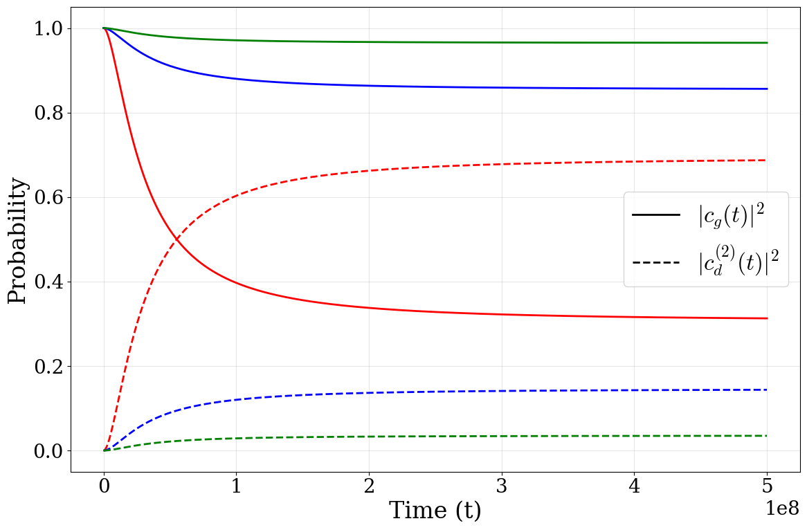
These considerations explain the main features in Fig. 7. For the pure growing initial state (blue), the warp primarily induces an admixture of $\ket{210}$, whose rate is typically much smaller in magnitude than $\Gamma_{211}$; hence even near $\Delta_{\rm res}\simeq 0$ the net change in $\Gamma_{\rm eff}$ remains modest. By contrast, mixed initial states (purple and green) activate the full three-level chain, so enhanced mixing near $\Delta_{\rm res}\simeq 0$ can pull significant weight into the decaying sector and produce a narrow suppression window. For a generic superposition (red), the same static reshuffling can either suppress or enhance $\Gamma_{\rm eff}$, depending on whether the warp rotates probability toward the growing or decaying eigen-combination at the chosen $\alpha$.

Figure 8: Ratio of effective growth rates with and without the warped-disk perturbation, $\Gamma_{\mathrm{eff}}^{\rm(warp)}/\Gamma_{\mathrm{eff}}^{(0)}$, highlighting the narrow region near $\Delta_{\rm res}(\alpha)\simeq 0$ where static mixing is strongest.

A complementary diagnostic is the ratio in Fig. 8, which makes the suppression or enhancement relative to the unperturbed case explicit and cleanly highlights where the static reshuffling is most efficient. The sharp feature near $\Delta_{\rm res}(\alpha)\simeq 0$ is the same mechanism in another guise: the effective splitting in the relevant channel becomes small, so the mixing amplitudes in Eq. (77) become parametrically enhanced. Strictly speaking, the nondegenerate expansion underlying Eq. (77) requires $|\bar{\Sigma}|\ll|\Delta_{g0}|,|\Delta_{0d}|$; therefore, extremely close to $\Delta_{\rm res}\approx 0$ one should diagonalize the appropriate near-degenerate sub-block. This refines the behavior at the very center of the window but does not change the qualitative conclusion that a static warp can generate a narrow suppression band in $\alpha$ for initial states that populate (or efficiently access) the decaying sector.

V Conclusion and discussion

We have investigated how the self-gravity of accretion disks of Kerr BH acts as an environmental perturbation to Kerr BH superradiance by reshaping the hydrogenic level structure and inducing mixing among the $n=2$ sublevels Brito et al. (2015); Arvanitaki and Dubovsky (2010). Focusing on the $\{\ket{211},\ket{210},\ket{21-1}\}$ subspace, we constructed an effective three-level description in which the disk enters through the quadrupolar ($\ell_{d}=2$) Newtonian potential. Two consistency conditions justify this treatment in the parameter regime of interest: (i) accretion-driven secular drifts of $M$ and $\Omega_{H}$ are slow compared to the linear superradiant growth, so the Kerr background can be treated as fixed during the growth epoch Baumann et al. (2019); Arvanitaki and Dubovsky (2010); and (ii) for $\alpha$ above the conservative working threshold, the disk potential in the cloud region is well captured by a low-$\ell$ multipole expansion, with $\ell_{d}=2$ providing the leading physical effect.

A central organizing principle is symmetry. The disk enters the perturbation as source multipoles $I_{d}^{(m_{d})}$ (projections onto $Y_{2m_{d}}$), while the angular selection rule $m_{d}=m^{\prime}-m$ determines which magnetic sublevels can couple. Breaking axial symmetry activates $m_{d}\neq 0$ channels, whereas breaking equatorial-reflection symmetry is required to activate the odd-parity $m_{d}=\pm 1$ quadrupole and thus involve the $\ket{210}$ state. Importantly, in both classes of perturbations the microscopic level-dependent rates $\Gamma_{21m}$ are unchanged; disk gravity modifies the effective growth rate only by redistributing probability weights among growing and decaying sublevels.

We illustrated these mechanisms using two representative disk configurations that isolate distinct symmetry-breaking channels:

(i) Equatorial spiral density waves (time-dependent, $m_{d}=\pm 2$). For a nonaxisymmetric but equatorially symmetric spiral perturbation, $\ket{210}$ decouples and the problem reduces to a driven two-level system $\ket{211}\leftrightarrow\ket{21-1}$. The spiral wave packet provides a coherent but transient drive: as the packet drifts outward the tidal coupling decays, leaving a late-time steady mixture set by the net population transfer. The outcome is controlled by the competition between the peak mixing rate and the driving detuning (equivalently by the control parameter $\Lambda$ introduced in the main text). This yields three qualitative regimes in the $(\alpha,\Sigma_{0})$ plane (Fig. 4): negligible mixing ($\chi\simeq 1$), suppressed growth ($0<\chi<1$), and a quench region ($\chi<0$) where ${\cal O}(1)$ transfer to the decaying partner can shut down superradiance. The suppression or quench behavior is most prominent in the small-$\alpha$ regime, where the intrinsic splitting is small and the cloud is more susceptible to disk-driven transitions.

(ii) Static warped disks (quasi-time-independent, $m_{d}=\pm 1$). For an axisymmetric but equatorially asymmetric warp, the leading effect in the small-tilt limit is the activation of the $m_{d}=\pm 1$ channel at ${\cal O}(\beta)$, producing genuine three-level mixing among $\{\ket{211},\ket{210},\ket{21-1}\}$. Because the perturbation is (quasi-)static, it does not act as a coherent drive; instead, it produces a static basis rotation: the cloud reorganizes into new stationary eigen-combinations whose composition is controlled by the ratio of the off-diagonal coupling $\bar{\Sigma}$ to the diagonal splittings $\Delta_{g0}$ and $\Delta_{0d}$. This naturally explains the features in Figs. 7 and  8: for a purely growing initial condition, the induced admixture is typically small, whereas for mixed initial states the full three-level chain is activated and the response becomes strongly initial-condition dependent. In particular, a narrow “growth gap” can appear when the effective splitting $\Delta_{\rm res}(\alpha)\equiv\Delta_{g0}=\epsilon_{h}-9\kappa\tilde{\Sigma}_{0}$ is accidentally suppressed, enhancing mixing and pushing $\Gamma_{\rm eff}$ toward very small or even negative values. The same static reshuffling can also yield enhancement of $\Gamma_{\rm eff}$ in certain regions of parameter space, reflecting the fact that a generic superposition may be rotated toward (rather than away from) the growing eigen-combination.

Taken together, our results show that disk gravity can qualitatively reshape the superradiant phenomenology even when it is perturbatively small: transient nonaxisymmetric structures (spirals) can act as time-dependent drives that suppress or quench growth, while quasi-static symmetry breaking (warps) can generate narrow suppression windows and state-dependent enhancement through three-level mixing. This implies that interpreting BH spin measurements and gravitational-wave searches in terms of ultralight-boson constraints requires accounting for plausible disk environments, especially in parameter regions where accidental near-degeneracies or near-resonant driving can amplify mixing.

Several extensions are natural. A more complete treatment would include larger level subspaces beyond $n=2$, model more realistic time-dependent disk dynamics (e.g. turbulence, recurrent spiral activity, and nonlinearly evolving warps), and incorporate nonlinear cloud physics (self-interactions and saturation). Near the centers of the suppression windows, a dedicated near-degenerate diagonalization can refine the detailed behavior, but the physical picture remains robust: disk-induced mixing reshuffles the cloud among growing and decaying components, thereby controlling the effective superradiant evolution in realistic astrophysical settings.

Appendix A Effective growth rate

According to Eq. (5), each eigenstate $\ket{n\ell m}$ is associated with a level-dependent growth/decay rate $\Gamma_{n\ell m}$. It is therefore convenient to introduce a rate operator $\hat{\Gamma}$ defined by

$$\hat{\Gamma}\ket{n\ell m}=\Gamma_{n\ell m}\ket{n\ell m}.$$ (A1)

The states $\ket{n\ell m}$ are eigenstates of $\hat{\Gamma}$. For a general superposition,

$$\ket{\psi}=\sum_{n,\ell,m}c_{n\ell m}\ket{n\ell m},$$ (A2)

an effective growth rate is defined as the expectation value of $\hat{\Gamma}$,

$$\Gamma_{\mathrm{eff}}=\braket{\psi|\hat{\Gamma}|\psi}=\sum_{n,\ell,m}|c_{n\ell m}|^{2}\Gamma_{n\ell m}.$$ (A3)

Appendix B Timescale for the evolution of the horizon angular velocity

Accretion proceeds through the inner disk and ultimately feeds the BH from the vicinity of ISCO Bardeen (1970). Both the BH mass $M$ and angular momentum $J$ therefore evolve, which in turn changes the horizon angular velocity $\Omega_{H}$ Thorne (1974); Shapiro and Teukolsky (1983).

The horizon angular velocity is given by

$$\Omega_{H}=\frac{a}{2Mr_{+}}=\frac{\tilde{a}}{2M(1+X)},\qquad X=\sqrt{1-\tilde{a}^{2}},$$ (B1)

where $\tilde{a}\equiv a/M$ is the dimensionless spin parameter. Taking a logarithmic time derivative yields

$$\frac{\dot{\Omega}_{H}}{\Omega_{H}}=\frac{\ \mathrm{d}}{\ \mathrm{d}t}\ln\Omega_{H}=\frac{\dot{\tilde{a}}}{\tilde{a}}-\frac{\dot{M}}{M}-\frac{1}{1+X}\dot{X}.$$ (B2)

Using $X=\sqrt{1-\tilde{a}^{2}}$ together with $\tilde{a}=J/M^{2}$, this expression can be rewritten as

$$\frac{\dot{\Omega}_{H}}{\Omega_{H}}=\frac{1}{X}\left(\frac{\dot{J}}{J}-\frac{2\dot{M}}{M}\right)-\frac{\dot{M}}{M}.$$ (B3)

The angular momentum inflow is related to the mass inflow through the specific angular momentum at the ISCO,

$$\dot{J}=l_{\mathrm{isco}}\,\dot{M},$$ (B4)

so that

$$\frac{\dot{J}}{J}=\frac{l_{\mathrm{isco}}}{\tilde{a}M}\frac{\dot{M}}{M}.$$ (B5)

Defining $\tilde{l}_{\mathrm{isco}}\equiv l_{\mathrm{isco}}/M$, the characteristic time scale for the evolution driven by accretion of $\Omega_{H}$ becomes

$$\tau_{\Omega}\equiv\frac{\Omega_{H}}{|\dot{\Omega}_{H}|}=\left|\frac{\tilde{a}\sqrt{1-\tilde{a}^{2}}}{\tilde{l}_{\mathrm{isco}}-\tilde{a}\left(2-\sqrt{1-\tilde{a}^{2}}\right)}\right|\frac{M}{\dot{M}}.$$ (B6)

In the above derivation, the ISCO specific angular momentum $l_{\mathrm{isco}}$ is obtained from Chandrasekhar (1998)

$$l=\frac{M^{1/2}\left(r^{2}\mp 2aM^{1/2}r^{1/2}+a^{2}\right)}{r^{3/4}\left(r^{3/2}-3Mr^{1/2}\pm 2aM^{1/2}\right)^{1/2}},$$ (B7)

evaluated at

$$r_{isco} =M\left(3+Z_{2}\mp\sqrt{(3-Z_{1})(3+Z_{1}+2Z_{2})}\right),$$ (B8)

$$Z_{1} =1+(1-\tilde{a}^{2})^{1/3}\left[(1+\tilde{a})^{1/3}+(1-\tilde{a})^{1/3}\right],$$

$$Z_{2} =\sqrt{3\tilde{a}^{2}+Z_{1}^{2}}.$$

Appendix C Spherical harmonics and symmetry constraints

The spherical harmonics are defined as

$$Y_{\ell m}(\theta,\phi)=N_{\ell m}P^{m}_{\ell}(\cos\theta)\,e^{im\phi}=\sqrt{\frac{2\ell+1}{4\pi}\frac{(\ell-m)!}{(\ell+m)!}}\,P^{m}_{\ell}(\cos\theta)\,e^{im\phi},\qquad m\in\mathbb{N},$$ (C1)

where $N_{\ell m}$ is a normalization constant and $P^{|m|}_{\ell}$ denotes the associated Legendre polynomials. Useful identities include

$$Y_{\ell m}(\pi-\theta,\phi)=(-1)^{\ell+m}Y_{\ell m}(\theta,\phi),$$ (C2)

and

$$Y_{\ell,-m}(\theta,\phi)=Y_{\ell m}^{\ast}(\theta,\phi)=Y_{\ell m}(\theta,-\phi).$$ (C3)

Consider the integral

$$I_{\ell m}^{m^{\prime}} =\int_{0}^{2\pi}Y_{\ell m}(\pi/2,\phi)\,e^{-im^{\prime}\phi}\,\mathrm{d}\phi$$

$$=N_{\ell m}P^{m}_{\ell}(0)\int_{0}^{2\pi}e^{i(m-m^{\prime})\phi}\,\mathrm{d}\phi.$$ (C4)

The associated Legendre polynomial at zero satisfies

$$P_{\ell}^{m}(0)=\begin{cases}0&\text{$\ell+m$ is odd},\\[4.0pt] \displaystyle(-1)^{(\ell+m)/2}\frac{(\ell+m-1)!!}{(\ell-m)!!}&\text{$\ell+m$ is even},\end{cases}$$ (C5)

and

$$\int_{0}^{2\pi}e^{i(m-m^{\prime})\phi}\,\mathrm{d}\phi=2\pi\,\delta_{mm^{\prime}}.$$ (C6)

Therefore, $I_{\ell m}^{m^{\prime}}$ is nonzero only if $m=m^{\prime}$ and $\ell+m$ is even.

For an equatorial disk, the source multipoles entering Eq. (45) take the form

$$I_{d}^{(m_{d})}=\sum_{m}\int_{r_{\mathrm{in}}}^{r_{\mathrm{out}}}\frac{\Sigma_{m}(t,r^{\prime})}{{r^{\prime}}^{2}}\int_{0}^{2\pi}Y^{\ast}_{2m_{d}}(\pi/2,\phi)\,e^{im\phi}\,\mathrm{d}\phi\equiv\sum_{m}\tilde{\Sigma}_{m}\cdot(I_{2m_{d}}^{m})^{\ast},$$ (C7)

where $\tilde{\Sigma}_{m}$ denotes the corresponding radial integral. For Eq. (C7) to be nonzero, one requires $2+m_{d}$ to be even, i.e. $m_{d}$ even. Combined with the selection rule, this implies that $m-m^{\prime}$ must be even, so $\ket{210}$ does not couple to the other two sublevels within the $\ell_{d}=2$ equatorially symmetric quadrupole perturbation.

This decoupling can also be understood from equatorial-reflection parity. Define the equatorial reflection operator $\mathcal{P}_{\mathrm{eq}}$ by

$$\mathcal{P}_{\mathrm{eq}}:\ \theta\to\pi-\theta,\qquad\phi\to\phi.$$ (C8)

If the disk is symmetric under equatorial reflection, then

$$\mathcal{P}_{\mathrm{eq}}V_{2}\mathcal{P}_{\mathrm{eq}}^{-1}=V_{2},$$ (C9)

so $V_{2}$ is even under $\mathcal{P}_{\mathrm{eq}}$. Using Eq. (C2), one finds

$$\mathcal{P}_{\mathrm{eq}}\ket{211} =\ket{211},$$

$$\mathcal{P}_{\mathrm{eq}}\ket{210} =-\ket{210},$$

$$\mathcal{P}_{\mathrm{eq}}\ket{21-1} =\ket{21-1}.$$

Thus $\ket{211}$ and $\ket{21-1}$ are even-parity states, while $\ket{210}$ is odd. As a representative example,

$$\bra{211}V_{2}\ket{210}=\bra{211}\mathcal{P}_{\mathrm{eq}}^{-1}\mathcal{P}_{\mathrm{eq}}V_{2}\mathcal{P}_{\mathrm{eq}}^{-1}\mathcal{P}_{\mathrm{eq}}\ket{210}=-\bra{211}V_{2}\ket{210},$$ (C10)

so the matrix element vanishes identically.

Appendix D Damping timescale for warp precession

Consider a geometrically thin Keplerian disk with a small tilt. The Lense–Thirring precession frequency Bardeen and Petterson (1975) is

$$\Omega_{\mathrm{LT}}(r)=\frac{2\tilde{a}M^{2}}{r^{3}}.$$ (D1)

Let $\bm{L}(r,t)$ denote the angular-momentum surface density Scheuer and Feiler (1996). In the Papaloizou–Pringle approximation the disk behaves approximately as a rigid body Papaloizou and Pringle (1983); taking the magnitude profile to be steady while allowing only the direction to evolve gives

$$\bm{L}(r,t)=L(r)\cdot\bm{l}(t),\qquad L(r)=\Sigma(r)\cdot r^{2}\Omega_{K}(r),\qquad\Omega_{K}=\sqrt{\frac{M}{r^{3}}}.$$ (D2)

An average precession frequency $\Omega_{p}$ is defined as Kumar and Pringle (1985)

$$\Omega_{p}=\frac{\int_{r_{\mathrm{in}}}^{r_{\mathrm{out}}}\Omega_{\mathrm{LT}}L\,\mathrm{d}r}{\int_{r_{\mathrm{in}}}^{r_{\mathrm{out}}}L\,\mathrm{d}r}\sim\mathrm{Const.}\cdot\int_{r_{\mathrm{in}}}^{r_{\mathrm{out}}}r^{-5/2}\,\mathrm{d}r.$$ (D3)

The inner region dominates, so a useful estimate is

$$\Omega_{p}\sim\Omega_{\mathrm{LT}}(r_{\mathrm{in}})=\frac{2\tilde{a}M^{2}}{r_{\mathrm{in}}^{3}}.$$ (D4)

Viscous dissipation damps the precession. A phenomenological estimate for the damping time scale is

$$\tau_{\mathrm{damp}}\sim\frac{R_{\ast}^{2}}{\nu_{2}}.$$ (D5)

Using $\nu_{2}=\alpha_{2}c_{s}H$ and $c_{s}=\Omega H$ gives Ogilvie (1999)

$$\tau_{\mathrm{damp}}\sim\frac{1}{\alpha_{2}\Omega(R_{\ast})}\left(\frac{R_{\ast}}{H}\right)^{2},$$ (D6)

and in the Papaloizou–Pringle approximation $\alpha_{2}\sim 1/(2\alpha)$.

Approximating $\Omega(R_{\ast})$ by $\Omega(r_{\mathrm{in}})$ yields

$$\frac{\tau_{\mathrm{damp}}}{T_{p}}\sim\tau_{\mathrm{damp}}\Omega_{p}=\frac{1}{\alpha_{2}}\frac{\Omega_{\mathrm{LT}}(r_{\mathrm{in}})}{\Omega(r_{\mathrm{in}})}\left(\frac{R_{\ast}}{H}\right)^{2}=\frac{2\tilde{a}}{\alpha_{2}}\left(\frac{M}{r_{\mathrm{in}}}\right)^{3/2}\left(\frac{R_{\ast}}{H}\right)^{2}.$$ (D7)

With the estimate $R_{\ast}\sim\sqrt{r_{\mathrm{in}}r_{\mathrm{out}}}$, one obtains

$$\frac{\tau_{\mathrm{damp}}}{T_{p}}\sim\frac{2\tilde{a}}{\alpha_{2}}\left(\frac{M}{r_{\mathrm{in}}}\right)^{3/2}\left(\frac{r_{\mathrm{out}}}{r_{\mathrm{in}}}\right)\left(\frac{r_{\mathrm{in}}}{H}\right)^{2},$$ (D8)

which is the estimate used in the main text.

Appendix E Geometric model for a warped disk

A geometrically thin warped disk can be modeled as a collection of rings. A ring at radius $r$ is obtained from the corresponding equatorial ring by a rotation about the $y$ axis by $\beta(r)$ followed by a rotation about the $z$ axis by $\gamma(r)$, with $\beta\ll 1$.

Consider a point on the equatorial ring,

$$P_{0}=(r\cos\phi,r\sin\phi,0)^{T}.$$ (E1)

After the two rotations, the corresponding point on the warped ring is

$$P=R_{z}(\gamma)R_{y}(\beta)P_{0}=\begin{pmatrix}r\cos\phi\cos\gamma-r\sin\phi\cos\beta\sin\gamma\\ r\cos\phi\sin\gamma+r\sin\phi\cos\beta\cos\gamma\\ r\sin\phi\sin\beta\end{pmatrix},$$ (E2)

where

$$R_{y}(\beta)=\begin{pmatrix}\cos\beta&0&-\sin\beta\\ 0&1&0\\ \sin\beta&0&\cos\beta\end{pmatrix},\qquad R_{z}(\gamma)=\begin{pmatrix}\cos\gamma&-\sin\gamma&0\\ \sin\gamma&\cos\gamma&0\\ 0&0&1\end{pmatrix}.$$ (E3)

Expanding Eq. (E2) to leading order in $\beta$ and rewriting it in spherical coordinates gives

$$P\simeq\begin{pmatrix}r\cos(\phi+\gamma)\\ r\sin(\phi+\gamma)\\ r\beta\cos\phi\end{pmatrix}=(r,\phi+\gamma,\arccos(\beta\cos\phi)).$$ (E4)

Therefore, when evaluating the warped-disk contribution to the gravitational potential, the equatorial expression can be used with the substitutions

$$\phi\to\phi+\gamma,\qquad\theta\to\arccos(\beta\cos\phi).$$ (E5)

Assuming an axisymmetric surface density $\Sigma=\Sigma(t,r^{\prime})$, the azimuthal integral appearing in Eq. (45) becomes

$$I_{\phi}^{(m_{d})}=\int_{0}^{2\pi}Y_{2m_{d}}^{\ast}(\arccos(\beta\cos\phi^{\prime}),\phi^{\prime}+\gamma)\,\mathrm{d}\phi^{\prime}.$$ (E6)

To the lowest relevant order in $\beta$,

$$I_{\phi}^{(\pm 2)} =-\frac{1}{8}\sqrt{\frac{15\pi}{2}}\beta^{2}\,e^{\mp 2i\gamma},$$ (E7)

$$I_{\phi}^{(\pm 1)} =\mp\frac{1}{2}\sqrt{\frac{15\pi}{2}}\beta\,e^{\mp i\gamma},$$ (E8)

$$I_{\phi}^{(0)} =\frac{1}{4}\sqrt{5\pi}(3\beta^{2}-2).$$ (E9)

Thus $I_{\phi}^{(\pm 2)}=\mathcal{O}(\beta^{2})$ while $I_{\phi}^{(\pm 1)}=\mathcal{O}(\beta)$. Retaining only terms linear in the small tilt implies that the $m_{d}=\pm 2$ contributions can be neglected at this order; by the selection rule, the $\ket{211}\leftrightarrow\ket{21-1}$ matrix element vanishes to $\mathcal{O}(\beta)$. In addition, $I_{\phi}^{(0)}\simeq-\sqrt{5\pi}/2$ at leading order.