CONE: Embeddings for Complex Numerical Data Preserving Unit and Variable Semantics

Abstract.

Large pre-trained models (LMs) and Large Language Models (LLMs) are typically effective at capturing language semantics and contextual relationships. However, these models encounter challenges in maintaining optimal performance on tasks involving numbers. Blindly treating numerical or structured data as terms is inadequate – their semantics must be well understood and encoded by the models. In this paper, we propose CONE, a hybrid transformer encoder pre-trained model that encodes numbers, ranges, and gaussians into an embedding vector space preserving distance. We introduce a novel composite embedding construction algorithm that integrates numerical values, ranges or gaussians together with their associated units and attribute names to precisely capture their intricate semantics. We conduct extensive experimental evaluation on large-scale datasets across diverse domains (web, medical, finance, and government) that justifies CONE’s strong numerical reasoning capabilities, achieving an F1 score of 87.28% on DROP, a remarkable improvement of up to 9.37% in F1 over state-of-the-art (SOTA) baselines, and outperforming major SOTA models with a significant Recall@10 gain of up to 25%.

1. Introduction

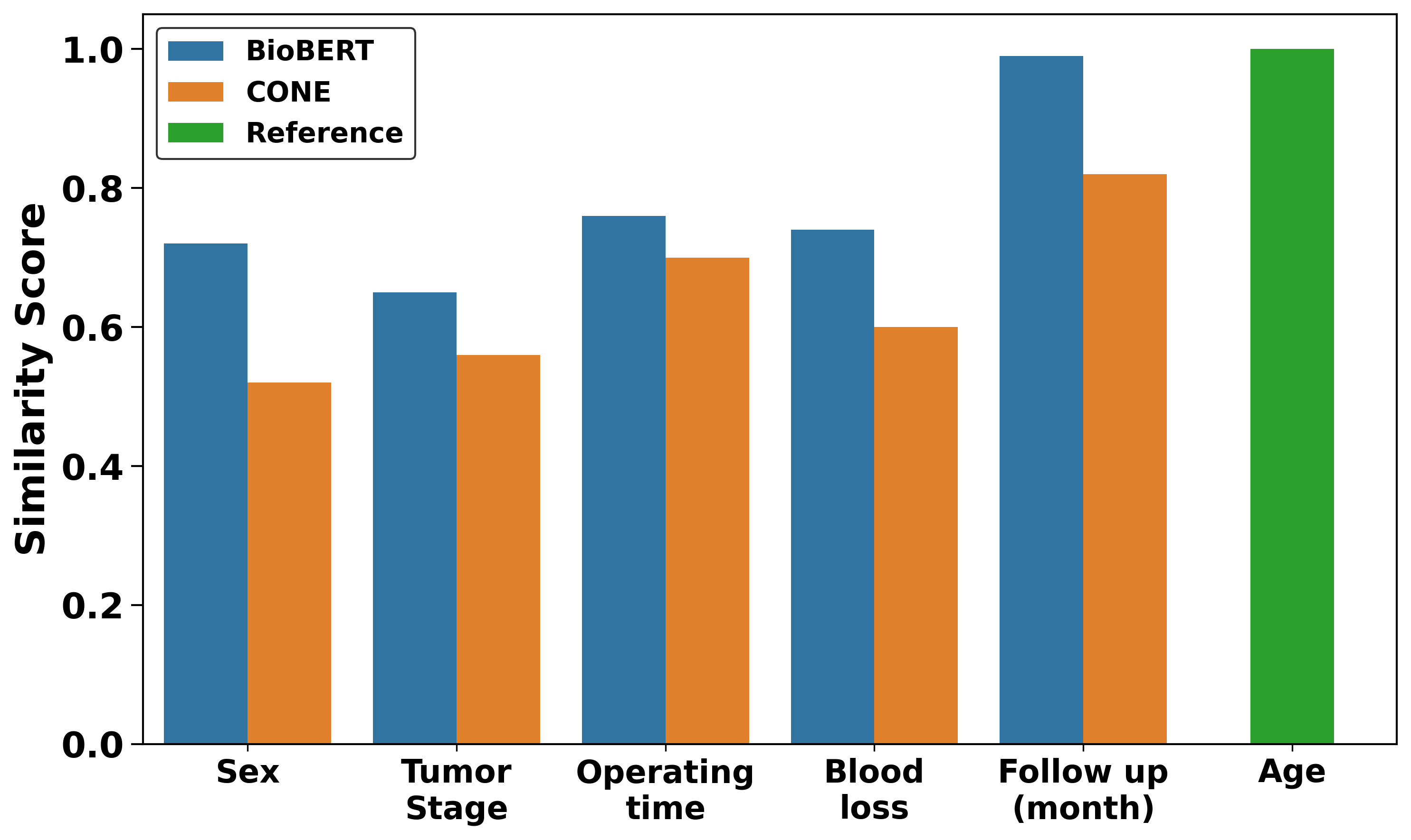
Natural language text typically contains both numerical values and words. Numerical data is especially ubiquitous and important in Science, Technology, Engineering, and Mathematics (STEM) fields, where precise numerical representations are critical. Numerical values can be expressed as digits (e.g., ‘15’), in alphabetic form (e.g., ‘fifteen’) both accompanied with units (e.g., ‘15 miles’). Units play a major role in correct comprehension and differentiation of quantities (e.g., 10 miles versus 10 kilograms). Numerical values in structured data carry additional semantics, such as being a value for a specific attribute and can also be accompanied by units. Despite the impressive performance of recent language models in natural language understanding (Devlin et al., 2019), they still struggle with tasks involving numerical and structured data. Multiple studies show that numerical embeddings from pre-trained LMs do not capture correctly the semantics of numerical values (Naik et al., 2019; Wallace et al., 2019; Devlin et al., 2019; Matthew, 2018; Zhang et al., 2020; Lee et al., 2020; Sundararaman et al., 2020; Yarullin and Isaev, 2023; Geva et al., 2020; Ran et al., 2019). One reason for this limitation stems from the tokenization strategies used in these models, which blindly treat numbers and words alike when deriving embedding vectors. For example, BERT (Devlin et al., 2019) uses a subword tokenization approach (Sennrich et al., 2016), which can split a number just like a word into several parts. Consider the number 28,600: it might be tokenized as “28” and “–600” completely distorting the original semantics. It is also important to note that different tokenizers can produce different segmentations. Finally, all these models overlook the fundamental differences between words and numbers as described in measurement theory (Stevens, 1946). Words are typically nominal (used for labeling without inherent order or magnitude), whereas numbers follow interval or ratio scales, where distance, order, and proportionality are crucial. Regular word embeddings capture the words’ semantic similarity, but lack mechanisms to correctly encode numerical data as well as fail to preserve its fundamental numerical properties. The issue becomes magnified by structured data that unlike 1D text has 2D-context, where numbers are associated with specific attributes. For example, two columns Age and Follow-up (month) in Figure 2 contain similar distributions of numbers, yet they are semantically distinct and that should be reflected in their corresponding vectorized representations. Pre-trained LMs often struggle to differentiate between such attributes (Figure 1), leading to poor performance in many numerical reasoning tasks.

Figure 1. Distance Between Age and Other Attributes, Calculated Using BioBERT and CoNE.

Table 1. CONE versus SOTA Models in Key Numerical Reasoning Capabilities and Support for Complex Numerical Data.

Features	BERT	ELMo	NumBERT	BioBERT	DICE	AeNER	GenBERT	NumNet	CONE
Numeration	limited	limited	yes	limited	yes	yes	yes	yes	yes
Magnitude	yes	yes	yes	yes	yes	yes	yes	yes	yes
List maximum	limited	better than BERT	-	limited	yes	yes	yes	yes	yes
Decoding	limited	better than BERT	-	Limited	yes	yes	yes	yes	yes
Addition	limited	limited	-	limited	yes	yes	yes	yes	yes
Scalar Probing	some	limited	good	limited	-	-	-	-	yes
Text	yes	yes	yes	yes	yes (as textual	yes	yes	yes	yes
					numbers)
Tabular Numerical Data	no	no	no	no	no	yes	no	no	yes

Age	Sex	Tumor Stage	Operating time	Blood loss	Follow-up (months)	BP (mmHg)	BMI (kg/$\text{m}^{2}$)
28	F	S1–3	7 hrs	3,000 mL	30	76-118	21.8 $\pm$ 2.9
34	F	S1–3	580 min	5 L	32	80-122	23.4 $\pm$ 3.2
36	F	S1–3	6 hrs	3.5 L	28	82-125	22.5 $\pm$ 3.17
42	M	S1–2	500 min	3,000 mL	25	85-130	24.1 $\pm$ 3.5
33	F	S1–3	400 min	3.2 L	20	78-120	22.2 $\pm$ 3.0
31	M	S1–2	500 min	3,000 mL	15	84-128	23.6 $\pm$ 3.4

Figure 2. A Table with Numerical Data Including Ranges and Gaussians Accompanied by Units.

Recently, numerical embeddings started gaining more attention (Zhang et al., 2020; Sundararaman et al., 2020; Yarullin and Isaev, 2023; Geva et al., 2020; Ran et al., 2019). Table 1 compares CONE with SOTA baselines. The comparison is based on reported results in the original papers and prior literature. None of these approaches fully capture semantics of numerical data having units, ranges, and gaussians. This fundamental limitation hinders their ability to fully comprehend and correctly encode complex numerical data found in text and structured data, where their semantics depend on the associated attributes and units (e.g., Age: 50 years vs. Weight: 50 kg).

To address these limitations, we describe CONE, a novel model for constructing composite embeddings that correctly encode and encapsulate semantics of complex numerical data including ranges and gaussians with units. CONE is built on top of pre-trained LMs, such as BERT (Devlin et al., 2019) and BioBERT (Lee et al., 2020) extending their capabilities to handle complex numerical semantics. By encoding numerical values within their complex structural context, this composite embedding approach ensures that numbers with differing units and/or attribute/variable, such as 5 km and 5 kg or 5 mg:dosage and 5 mg:weight, are not being blindly treated alike, even though their numerical value is identical (5). On top of that, CONE comprehends and encodes correctly semantics of numerical ranges (e.g., [5-10 years]:Age) and gaussians (e.g., [1302±0.25 nm, mean $\pm$ SD]:Particle Size) correctly allowing the model not to lose their real semantics. Through extensive experiments on popular downstream tasks with complex structured data we demonstrate that CONE significantly outperforms the widely used SOTA baselines, such as TAPAS (Herzig et al., 2020), NumNet (Ran et al., 2019), NC-BERT (Kim et al., 2022), Magneto (Liu et al., 2025) and general-purpose embedding models (Chen et al., 2024; Zhang et al., 2024, 2025; Hu et al., 2025). By incorporating unit-aware and attribute-specific embeddings, our model ensures that complex numerical data is represented correctly, improving both retrieval and predictive downstream tasks.

Our key contributions are as follows:

• Novel composite embedding structure for complex numerical data that incorporates the numerical value, unit, and attribute, allowing the model to accurately encode and comprehend numbers with their complex associated contexts. This ensures that numbers with different units and attributes are distinct and the encoding preserves their fundamental numerical properties.

• Special embeddings for numerical ranges and gaussians preserving their semantics.

• Two novel algorithms for the embedding vector components pre-computation (Algorithm 1) and complete embedding vector composition (Algorithm 2).

• Extensive experimental evaluation of CONE on large-scale datasets from different domains, demonstrating its superior performance on popular downstream tasks.

The rest of the paper is structured as follows. We begin with preliminaries, then describe our methodology, followed by rigorous embedding distance analysis, extensive experimental evaluation, related work, and conclusion.

2. Preliminaries

While language models demonstrate impressive performance on capturing textual semantics, they remain limited in their ability to capture the semantics of numerical values or complex structured data, where numbers inherit their semantics from the attribute (e.g., Age, Dose, BMI), the units in which they are expressed (years, mg, kg/$\text{m}^{2}$), and the structure of the numerical values themselves (single value, ranges, or gaussians). A numerical value, such as “30” may correspond to 30 years of age, 30 months of follow-up, or 30 mm of tumor size; its meaning depends entirely on its associated attribute and unit. Standard language models (e.g., BioBERT) do not encode these distinctions correctly, hence may confuse attributes that are numerically identical or lexically similar, but semantically different.

Let a table be $T=(C,R)$, where $C=\{c_{1},\dots,c_{m}\}$ is the set of $m$ columns with attribute names $A=\{a_{1},\dots,a_{m}\}$, and $R=\{r_{1},\dots,r_{n}\}$ is the set of $n$ tuples with $r_{i}=[v_{i1},\dots,v_{im}]$ the corresponding cell values.

Definition 1 (Column Similarity). Two columns $c_{1}$ and $c_{2}$ are similar iff they have similar attribute values (Hasan and Ferdous, 2024). We describe the column similarity measure more precisely below.

Each column $c_{j}$ contains attribute values $\{v_{1j},\dots,v_{nj}\}$. For each $v_{ij}$, we compute a composite embedding $E^{\text{comp}}(a_{j},v_{ij},u)$ (Algorithm 2) that encodes the attribute name $a_{j}$, $v_{ij}$, and unit $u$. The embedding vector of column $c_{j}$ is then obtained by aggregation:

(1) $$\footnotesize{E}(c_{j})=\sum_{i=1}^{n}E^{\text{comp}}(a_{j},v_{ij},u)$$

Similarity between two columns $c_{1}$ and $c_{2}$ is computed by calculating the cosine of the angle between their aggregated embedding vectors (Hasan and Ferdous, 2024):

(2) $$\footnotesize Sim_{{col}}(c_{1},c_{2})=\cos\big(E(c_{1}),E(c_{2})\big)$$

Definition 2 (Tuple Similarity). Two tuples $r_{1}$ and $r_{2}$ are similar iff they have similar cell values. We describe the tuple similarity measure more precisely below.

Each tuple $r_{i}=[v_{i1},\dots,v_{im}]$ consists of cell values $v_{ij}$ corresponding to each attribute $a_{j}\in A$. The embedding of tuple $r_{i}$ is obtained by aggregation:

(3) $$\footnotesize{E}(r_{i})=\sum_{j=1}^{m}E^{\text{comp}}(a_{j},v_{ij},u)$$

Similarity between two tuples $r_{1}$ and $r_{2}$ is computed by calculating the the cosine of the angle between their aggregated embedding vectors:

(4) $$\footnotesize Sim_{{tuple}}(r_{1},r_{2})=\cos\big(E(r_{1}),E(r_{2})\big)$$

Example 1. Consider a table in Figure 2. ‘Age (years)’ can be stored as {28, 34, 36, 42, 33, 31}, {29, 31, 35, 42, 32, 32}, or as a range such as “30–45”. Despite different representation, these belong to the same demographic concept and must therefore be embedded close to each other in the vector space. In contrast, attributes such as ‘Follow-up Duration (months)’ with values {20, 25, 30, 36, 40, 32} or Tumor Size (mm) with values {30, 35, 42, 22, 26, 32} may numerically overlap with ‘Age’, but encode completely different variables. Hence, they should not be positioned close to ‘Age’ in the embedding vector space. The only attributes that should exhibit high similarity to ‘Age’ in Figure 1 are other attributes that may contain some ‘Age’ values. The attributes, such as ‘Follow-up’, or ‘Operating Time’ must remain well separated, regardless of any numeric overlap due to their different semantics.

We can see in Figure 1 that BioBERT cannot distinguish Age and Follow-up(month) originating from the table in Figure 2. Their cosine similarity score is $0.9998$, hence the angular distance is very small - $1.02^{\circ}$, which means that these two vectors constructed by BioBERT nearly overlap with each other. This is due to very similar distributions of numerical values from these two columns, and ”blindness” of vanilla BERT embedding vectors to differences in units and attributes (i.e. lack of numerical and unit semantics). BioBERT’s high similarity scores are driven primarily by textual similarity between attribute names (e.g., month appearing semantically similar to Age) rather than by the more intricate semantics of the numerical values. Not only BERT and BioBERT, but also other SOTA general-purpose embedding models (Chen et al., 2024; Zhang et al., 2024, 2025; Hu et al., 2025) do not perform well on tasks involving numbers, also because they treat numbers as regular terms.

In large-scale datasets, this issue is exacerbated by attribute heterogeneity and data representation variety. The tables come from a myriad of different sources, which use different naming conventions, schemata, formats. Further, they use different synonyms, abbreviations in tables’ headers, which complicates the problem. There will also be variance in both textual and numerical data formats for the same attributes, which poses additional challenges constructing the embeddings correctly mimicking the data semantics. To overcome these challenges we propose a more complex – composite structure for the embedding vectors and a modified encoder architecture that accurately encode semantics of complex numerical data.

Definition 3 (Serialization). At a column-level, we serialize each column $c_{j}$ independently as: $\mathcal{S}_{\text{col}}(c_{j})\mathrel{\mathop{:}\!\text{-}}[\text{CLS}]\,a_{j}\,[\text{SEP}]\,v_{1j}\,[\text{SEP}]\,\\ \dots\,v_{nj}\,[\text{SEP}]$. I.e., we place the column name first, followed by all cell values, using [SEP] tokens to delimit values and a single [CLS] token at the start (where [CLS] and [SEP] follow the BERT tokenization standard (Devlin et al., 2019)). At a tuple-level, we serialize a row $r_{i}$ as $\mathcal{S}_{\text{row}}(r_{i})\mathrel{\mathop{:}\!\text{-}}[\text{CLS}]\,a_{1}\,v_{i1}\,[\text{SEP}]\,\dots a_{m}\,v_{im}\,[\text{SEP}]$. I.e., each attribute name is interleaved with its corresponding cell value and attribute–value pairs are separated by [SEP] tokens.

We experimented with multiple alternative serialization strategies, which proved less effective. For consistency, we use the same serialization for BioBERT and other models in our experiments. Throughout the paper, we use the term attribute to refer to a column header (i.e., the column name), whereas column denotes the entire column, including both the header and its cell values.

Example 2. Consider the tuples and columns in the table shown in Figure 2. We serialize the column with attribute ‘Age’ in the table as: [CLS]  Age  [SEP]  28  [SEP]  34  [SEP]  36  [SEP]  42  [SEP]  33  [SEP]  31  [SEP]. Similarly, we serialize the tuple (the first row) in the table as: [CLS]  Age 28  [SEP]  Sex F   [SEP]  Tumor Stage S1-3  [SEP]  Operating time 7 hrs  [SEP]  Blood loss 3000 mL  [SEP]  Follow-up (month) 30  [SEP]  BP (mmHg) 76-118  [SEP] BMI (kg/$\text{m}^{2}$) 21.8 $\pm$ 2.9  [SEP].

We modified BERT architecture (Devlin et al., 2019; Lee et al., 2020) to accommodate advanced semantics of complex numerical data having units, numbers, ranges, and gaussians. Each Transformer layer includes a multihead self-attention sub-layer, where each token attends to all the tokens. Let the layer input ${H}=[h_{1},h_{2},\dots,h_{n}]^{T}\in\mathbb{R}^{n\times d}$ correspond to sequence $S$, where $d$ is the hidden dimension, and $h_{i}\in\mathbb{R}^{d\times 1}$ is the hidden representation at position $i$. For a single-head self-attention sub-layer, the input $H$ is projected by three matrices ${W}^{Q}\in\mathbb{R}^{d\times d_{K}}$, ${W}^{K}\in\mathbb{R}^{d\times d_{K}}$, and ${W}^{V}\in\mathbb{R}^{d\times d_{V}}$ to the corresponding representations $Q$, $K$, and $V$:

(5) $$Q=H{W}^{Q},\quad V={H}{W}^{V},\quad{K}={H}{W}^{K}$$

Then, the output of this single-head self-attention sub-layer is calculated as:

(6) $$\text{Attn}({H})=\text{softmax}\left(\frac{{Q}{K}^{T}}{\sqrt{d_{K}}}\right){V}$$

As illustrated in Figure 1, our method reduces the similarity between Age and Follow-up to 0.82. When ranking column similarity to Age, our method places all Age-related columns at the top, while Follow-up does not appear among the top candidates. Our method is explicitly designed to encode such distinctions by jointly capturing attribute, unit, and numerical values, ensuring that semantically equivalent numerical attributes are embedded closely while semantically different ones remain well separated. Likewise another source of ambiguity arises when attributes share the same name, but use incompatible units. For instance, the attribute Dose may refer to 40–60 mg (drug mass), 4–6 mL (drug volume), or 1.0–1.5 IU/kg (biological potency). Text-based embeddings consider these nearly the same, because the term ‘Dose’ dominates their embedding representation and the unit mismatch is not considered. Our method incorporates unit semantics explicitly, ensuring that Dose (mg), Dose (mL), and Dose (IU/kg) are embedded as distinct concepts. Our embedding representation is general-purpose and does not require any modification for different downstream tasks.

3. CONE Model

Our model architecture is illustrated in Figure 3. It enhances standard transformer encoders with numerically-aware embeddings, improving the model’s ability to understand and reason about numerical values.

Figure 3. CONE Architecture including the Encoder and Numerical Value Embeddings. The Encoder Embeddings for Numbers ($M^{E}$, shown in blue) are Fused with Numerical Value Embeddings ($M^{N}$, pink) and Refined Through a Transformer to Produce the Contextualized Representations ($M^{O}$, green).

3.1. Encoder

We adopt a transformer-based language model as the encoder (Devlin et al., 2019; Yarullin and Isaev, 2023), initialized with BioBERT (Lee et al., 2020) weights and fine-tuned on our datasets. In this work, we focus on numerical columns/tuples in tables. The input to the encoder is a tokenized concatenation of [CLS], and table’s tuple or column, where the table is flattened along row/column and the cells are separated by the [SEP] token using a serialization function $\mathcal{S}$ (see Definition 3). Given a tokenized input sequence of length $l$, the encoder generates a corresponding contextualized representation denoted as:

(7) $${E}^{E}=[e_{1},e_{2},\dots,e_{l}]\in\mathbb{R}^{l\times d}$$

where $d$ represents the embedding dimension (we use $d=768$ throughout).

We do not modify the default tokenizer of the underlying encoder for textual tokens, which therefore follow the standard tokenization process (Lee et al., 2020). However, we override the tokenizer’s behavior for numberical data (see Section 3.2): each number is treated as a single token, rather than being split into multiple subword tokens as in BERT/BioBERT, whenever no corresponding embedding exists. The embedding for each numerical token is learned through our custom architecture in Figure 3.

3.2. Embeddings for Numerical Values

We propose numerical fusion embeddings that jointly capture symbolic context and quantitative magnitude. This is achieved by augmenting the standard token embeddings of numerals with numerical value embeddings (Sundararaman et al., 2020; JIN et al., 2023; Berg-Kirkpatrick and Spokoyny, 2020; Spithourakis and Riedel, 2018; Gorishniy et al., 2022; Thawani et al., 2021) and integrating them through attention (Yarullin and Isaev, 2023). Although we focus on encoder-based models in this work, the CONE framework is not architecture-specific. The numerical attention fusion mechanism can be applied to both encoder and decoder architectures by replacing their token embeddings with the fused representation, followed by the lightweight transformer block for number-specific reasoning.

We extract numeric tokens (i.e. numerals) from the input (e.g. column or row) and use DICE (Sundararaman et al., 2020) to generate numerical value embeddings $M^{N}$, one component of our embedding vector that enhances the representation of numerical properties (e.g., magnitude). One can also use other existing methods (JIN et al., 2023; Berg-Kirkpatrick and Spokoyny, 2020; Spithourakis and Riedel, 2018; Gorishniy et al., 2022; Thawani et al., 2021).

Let ${I}^{\text{num}}=\{i_{1},i_{2},\dots,i_{s}\}$ be the set of indices of numeric tokens. Each index corresponds to the relative position of a numeral token in the input sequence. For each $i_{j}\in I$, we retrieve the corresponding encoder embedding from $E^{E}$ and denote the subset of these embeddings ${M}^{E}\in\mathbb{R}^{s\times d}$ as follows:

(8) $$M^{E}_{j}=e_{i_{j}},\quad\text{for }j=1,\ldots,s$$

We compute a fused representation by element-wise summation of the contextual embeddings ${M}^{E}$ and the numerical value embeddings ${M}^{N}$, and feed the result into a transformer block to enable number-specific reasoning. The resulting output ${M}^{O}$, which provides contextualized embeddings for each numeral token, is then used to update the corresponding embeddings in the encoder output ${E}^{E}$. This yields the final embedding ${E}^{O}$, which incorporates both contextual and numerical semantics.

Figure 4. Composite Embedding Structure for (a) Complex Numerical Data, (b) Numerical Ranges, and (c) Gaussians. T: Text, N: Numerical Value, SD: Standard Deviation.

1: Input: Tokenized input $x=[x_{1},\dots,x_{l}]$; encoder $f_{\theta}$ (initialized with BioBERT); numerical value embedding $\text{NumEmbed}(\cdot)$; transformer block $g_{\phi}$; masking ratio $p$; Adam optimizer $\mathcal{O}$

2: Output: Trained parameters $\theta$ and $\phi$

3: $I^{\text{num}}\leftarrow\{i\in[1..l]\mid x_{i}\text{ is a numeral}\}$ // indices of numeral tokens

4: $\tilde{x}\leftarrow\text{MaskNumerals}(x,I^{\text{num}},p)$ // replace subset with [MASK]

5: $E^{E}\leftarrow f_{\theta}(\tilde{x})\in\mathbb{R}^{l\times d}$ // contextual embeddings

6: $M^{E}\leftarrow[E^{E}_{i}]_{i\in I^{\text{num}}}\in\mathbb{R}^{s\times d}$ // $s=|I^{\text{num}}|$

7: $M^{N}\leftarrow[\text{NumEmbed}(x_{i})]_{i\in I^{\text{num}}}\in\mathbb{R}^{s\times d}$

8: $M^{F}\leftarrow M^{E}+M^{N}$ // fusion by element-wise sum

9: $M^{O}\leftarrow g_{\phi}(M^{F})$ // number-specific reasoning

10: $(\hat{y},\hat{c})\leftarrow\text{Heads}(M^{O})$ // magnitude $\hat{y}$ and class $\hat{c}$

11: $(y,c)\leftarrow\text{GroundTruthMagnitudesAndClasses}(x,I^{\text{num}})$

12: $\mathcal{L}_{\text{mag}}\leftarrow\sum_{j=1}^{s}(\log y_{j}-\log\hat{y}_{j})^{2}$

13: $\mathcal{L}_{\text{cls}}\leftarrow\sum_{j=1}^{s}\text{CEL}(c_{j},\hat{c}_{j})$

14: $\mathcal{L}_{\text{num}}\leftarrow\mathcal{L}_{\text{mag}}+\mathcal{L}_{\text{cls}}$

15: $\theta,\phi\leftarrow\mathcal{O}(\theta,\phi,\nabla_{\theta,\phi}\mathcal{L}_{\text{num}})$

16: return Updated parameters $\theta$ and $\phi$

Algorithm 1 CONE Training via Masked Numeral Prediction

We train the model using a masked numeral prediction task (Spithourakis et al., 2016; Lin et al., 2020; Sakamoto and Aizawa, 2021), as outlined in Algorithm 1, where the model is trained to predict a masked numeral in the input. The objective function $\mathcal{L}_{\text{num}}$ (Equation 9) combines magnitude regression with classification loss:

(9) $$\mathcal{L}_{\text{num}}=\sum_{i=1}^{N}\left\{\left(\log(y_{i})-\log(\hat{y}_{i})\right)^{2}+\text{CEL}_{i}\right\}$$

where, $y_{i}$ denotes the ground-truth numerical magnitude, $\hat{y}_{i}$ is the magnitude of the numeral predicted by the model, $N$ is the number of masked numerals in the training, and $\text{CEL}_{i}$ is the cross-entropy loss for the $i$-th numeral token. After training, the numeral prediction head is discarded, and the final contextualized embedding $E^{O}$ is used for various downstream tasks. $E^{O}$ encodes numerals both in terms of their semantic role (context) and their quantitative value on the number line (magnitude).

3.3. Composite Embedding Structure

Prior studies (Yin and Schütze, 2016; Xu et al., 2018; Bollegala, 2022; Liu et al., 2015, 2019b; Wang et al., 2021b; Matthew, 2018) show that concatenated embeddings outperform single embeddings on tasks such as similarity and classification. Importantly, concatenation (CONC) retains each embedding in its original subspace, preserving source information without forcing it into a single space. This yields representations that are both expressive, by integrating complementary signals, and discriminative (e.g., Age = 50 years vs. Weight = 50 kg, where the identical value “50” is distinguished by attribute and unit context). Motivated by this, we propose a composite embedding structure that concatenates ($\oplus$) embeddings $E^{O}$ (see Figure 3) for the attribute, its value (scalar, range, or Gaussian), and the unit, thereby preserving the complementary contributions of each component to structured numerical data. Our composite embedding corresponds to combination of subspaces (Halmos, 2017), ensuring that each component (attribute, value, unit) contributes independently to the overall distance (see Section 5 for a detailed distance analysis). For instance, when the attribute and unit are fixed, distances between composites reduce to differences in the value, so vector distances naturally reflect numeric proximity; the same property holds when either the attribute or the unit is fixed.

Figure 4(a) illustrates this process for a column Blood loss from the table in Figure 2, attribute Blood loss has value “3,000” in the first row, and the unit “mL” is specified along with the value. This composite embedding structure preserves the actual semantics of the numerical value. We call Range (a-b) an interval that includes all $x$ between two boundaries a and b, such that $a\leq x\leq b$. To construct the composite embedding for numerical Range values (e.g., Age 1–5 years), we represent each range using its center $\tfrac{a+b}{2}$ and length $|b-a|$, which provide an orthogonal representation of the range’s location and scale. The composite embedding is then obtained by concatenating the embeddings for the attribute, center, length, and unit. In Figure 4(b) we show this composite structure for BMI (i.e. Body Mass Index) “18-24” kg/$\text{m}^{2}$. For brevity, we call Gaussian - a Gaussian distribution $mean\pm SD$ with $mean$ and SD, where SD denotes the Standard Deviation. The composite embedding for Gaussian values has similar structure to that of Range, where we concatenate the embeddings for the attribute, “$mean-SD$”, “$mean$”, “$mean+SD$”, and unit. Figure 4(c) illustrates this structure using the example attribute PS (nm) (Particle Size) with the value “$1302\pm 0.25$”.

CONC embeddings have dimensionality proportional to the number of components (i.e., $k\cdot d$ for $k$ components). To avoid high and variable dimensionality in CONC and obtain a fixed-size representation, we adopt a slot-based concatenation scheme with zero padding and masking. We reserve a fixed set of slots $\mathcal{S}$ ($|\mathcal{S}|=5$ in our case), each of size $d$. Missing components are zero padded, and the corresponding binary mask bit is set to $m_{s}=0$. Concatenating all slots yields $E\in\mathbb{R}^{|\mathcal{S}|d}$, which is then projected to a vector space with dimension $d_{C}=768$ using a linear autoencoder (Baldi and Hornik, 1989; Baldi, 2012). The reconstruction is $\hat{E}=W^{\top}WE$, where $W\in\mathbb{R}^{d_{C}\times(|\mathcal{S}|d)}$ denotes the encoder projection matrix and $W^{\top}$ the tied decoder, and training minimizes the masked reconstruction loss (Vincent et al., 2008; He et al., 2022).

(10) $$\mathcal{L}_{\text{embed}}=\|M\odot(\hat{E}-E)\|_{2}^{2}$$

where $M\in\{0,1\}^{|S|d}$ is the broadcast mask derived from $\{m_{s}\}_{s\in\mathcal{S}}$, and $\odot$ denotes the Hadamard (element-wise) product. The encoded representation $z=WE$ is layer-normalized to produce the final composite embedding:

(11) $$E^{\text{comp}}=\mathrm{LayerNorm}(z)$$

1: Input: Attribute $a$, numeric value $v$ (scalar, range $[a,b]$, or Gaussian $(\mu,\sigma)$), unit $u$, slot size $d$, total slots $|S|$, projection matrix $W$

2: Output: Composite embedding $E^{\text{comp}}$

3: if $a$ exists then $E_{a}\leftarrow\text{CONE}(a)$ else $E_{a}\leftarrow\text{ZeroPad}(d)$ end if

4: if $v$ is scalar then $E_{v}\leftarrow\text{CONE}(v)$

15: else if $v$ is range $(a,b)$ then

$E_{v}\leftarrow\text{Concat}(\text{CONE}(\tfrac{a+b}{2}),\text{CONE}(|b-a|))$

26: else if $v$ is Gaussian $(\mu,\sigma)$ then

$E_{v}\leftarrow\text{Concat}(\text{CONE}(\mu-\sigma),\text{CONE}(\mu),\text{CONE}(\mu+\sigma))$

7: else $E_{v}\leftarrow\text{ZeroPad}(d)$ end if

8: if $u$ exists then $E_{u}\leftarrow\text{CONE}(u)$ else $E_{u}\leftarrow\text{ZeroPad}(d)$ end if

9: Concatenate embeddings: $E\leftarrow[E_{a},E_{v},E_{u}]$ into $|S|$ slots of size $d$

10: Zero-pad unused slots and build binary mask $M$

11: Project: $z\leftarrow WE$ // linear autoencoder projection

12: Reconstruct: $\hat{E}\leftarrow W^{\top}z$

313: Compute masked reconstruction loss: $L_{\text{embed}}\leftarrow\|M\odot(E-\hat{E})\|^{2}_{2}$

-8pt

14: Normalize: $E^{\text{comp}}\leftarrow\text{LayerNorm}(z)$

15: return $E^{\text{comp}}$

Algorithm 2 Composite Embedding Construction

In our implementation, attribute names $a$, numerical values $v$, and unit symbols $u$ are extracted from tabular data for each row or column using a rule-based and regular-expression parser adapted from (Ceritli and Williams, 2021). The method in (Ceritli and Williams, 2021) also supports unit canonicalization, which normalizes all unit variants into a consistent canonical form. The resulting triplet $(a,v,u)$ is then used to construct the composite embedding as described in Algorithm 2.

4. Datasets

We use the following five publicly available large-scale datasets in our experiments and we used the methods from (Kandibedala et al., 2025) for complex metadata identification, which involves detecting multi-row, hierarchical headers and Bi-dimensional headers (i.e., columns and rows with metadata). This facilitates the construction of large-scale training and test sets for our experiments (Section 6.3).

CancerKG (Shrestha et al., 2025) dataset has 3.5M tables, extracted from all recent medical publications (up to year 12/2024) on different cancers, obtained via PubMed.com. The tables have 19.75M columns and 18.44M tuples total. The column/tuple values contain strings, numbers with and without units, ranges. CovidKG (Shrestha et al., 2025) is extracted from medical publications (up to year 2022) on COVID-19, obtained via PubMed.com. It contains 0.82M papers and 1.4M tables. Webtables (Lehmberg et al., 2016) contains around 1.65M tables extracted from Wikipedia pages. The corpus contains a large amount of factual knowledge on various topics ranging from sport events (e.g., Olympics) to artistic works (e.g., TV series). CIUS (Gol et al., 2019) dataset is from the Crime In the US (CIUS) database and consists of 1,050 tables with information about crime offenses. SAUS (Gol et al., 2019), the 2010 Statistical Abstract of the United States (SAUS) from the U.S. Census Bureau comprises 1,368 tables covering topics like finance, business, crime, agriculture, and health.

We also evaluate our model on DROP dataset (Dua et al., 2019), a question answering (QA) benchmark that tests numerical reasoning skills such as counting, sorting, and addition. It contains 77,409 training, 9,536 development, and 9,622 test question–answer pairs. In addition, we use six datasets GDC, Magellan, WikiData, Open Data, ChEMBL and TPC-DI from (Liu et al., 2025; Koutras et al., 2021) to evaluate and compare with recent schema matching (SM) solutions (Liu et al., 2025; Du et al., 2024). Due to space constraints we refer the reader to (Liu et al., 2025; Koutras et al., 2021) for statistics on these datasets.

5. Analysis of Distance

Table 2. Correlation of Analytic Distances (Section 5.1) with Embedding Cosine Distances via Pearson’s $r$ and Spearman’s $\rho$.

	Numbers		Ranges				Gaussians
	Abs. Diff.		Euclidean		Jaccard IoU		Wasserstein
Method	$r$	$\rho$	$r$	$\rho$	$r$	$\rho$	$r$	$\rho$
BioBERT	0.067	0.064	0.398	0.355	0.267	0.248	0.038	0.039
CONE	0.989	0.798	0.997	0.786	0.498	0.465	0.689	0.663

To validate our composite embeddings for complex numerical data we check that each of its three components separately is contributing to the distance as expected. Hence, we separately evaluated the effectiveness of fine-tuned embeddings for the number values, units, and attributes.

The Euclidean distance (Lee et al., 2012) between two CONE embedding vectors for numbers $\mathbf{x}=[x_{1},y_{2},\ldots,x_{d}]$ and $\mathbf{y}=[y_{1},y_{2},\ldots,y_{d}]$ is:

(12) $$D_{xy}=\sqrt{\sum_{i=1}^{d}(x_{i}-y_{i})^{2}}$$

5.1. Analytic distance metrics

We define the distances used to evaluate number, range, and Gaussian embeddings.

5.1.1. Numbers (absolute difference)

For two scalars $x,y\in\mathbb{R}$, the distance is

(13) $$d_{\text{num}}(x,y)=|x-y|$$

5.1.2. Ranges

For two ranges $R_{i}=[a,b]$ and $R_{j}=[c,d]$, we consider two distances:

Euclidean distance (Lee et al., 2012): Center and length are defined as $c_{i}=\tfrac{a+b}{2},\;\ell_{i}=|b-a|$ and $c_{j}=\tfrac{c+d}{2},\;\ell_{j}=|d-c|$, and the distance is

(14) $$d_{\text{CL}}(R_{i},R_{j})=\sqrt{(c_{i}-c_{j})^{2}+(\ell_{i}-\ell_{j})^{2}}$$

Jaccard-based Intersection over Union (IoU) distance (Niwattanakul et al., 2013):

(15) $$d_{\text{IoU}}(R_{i},R_{j})=1-\frac{|R_{i}\cap R_{j}|}{|R_{i}\cup R_{j}|}$$

where the intersection length is $\max(0,\min(b,d)-\max(a,c))$ and the union length is $(b-a)+(d-c)-|R_{i}\cap R_{j}|$.

5.1.3. Gaussians (2-Wasserstein distance)

For two Gaussians $\mathcal{N}(\mu_{i},\sigma_{i}^{2})$ and $\mathcal{N}(\mu_{j},\sigma_{j}^{2})$ the distance is (Peyré et al., 2019),

(16) $$d_{\mathcal{W}_{2}}(i,j)=\sqrt{(\mu_{i}-\mu_{j})^{2}+(\sigma_{i}-\sigma_{j})^{2}}$$

Figure 5. Euclidean Distance from Embedding of 0 to the Embeddings of Numbers from 0 to 100

.

5.2. CONE Embedding Components

5.2.1. Numbers

In Figure 5, we plot the pairwise Euclidean distances for CONE embedding vectors corresponding to 0 and numbers from 0 to 100. As the numbers increase, the distances grow accordingly as expected, demonstrating CONE’s ability to capture numerical magnitude, effectively encoding both order and interval properties (Stevens, 1946). The distance is monotonically increasing (larger numbers map farther away from 0), but starts demonstrating monotonic non-linearity with growth. Due to space, we show here the results for numbers from 0 to 100, however the same dynamics remains for much larger numbers (i.e. $\approx$1000) as well according to our experiments. We also evaluate whether embeddings preserve actual distances of numbers (scalars, ranges, and gaussians) by comparing these distances (Section 5.1) with corresponding distances in the embedding space. We report Pearson’s correlation coefficient ($r$) for linear association and Spearman’s rank correlation coefficient ($\rho$) for rank-order consistency (Lee Rodgers and Nicewander, 1988). Results are summarized in Table 2. Quantitatively, correlating absolute differences of numbers (from 0–1000) with their corresponding embedding cosine distances yields weak correlation for standard encoder embeddings (e.g., BioBERT; $r\!\approx\!0.07$, $\rho\!\approx\!0.06$), while CONE achieves strong correlation ($r\!=\!0.989$, $\rho\!=\!0.798$). This shows that CONE preserves numerical magnitude, unlike standard encoders.

5.2.2. Ranges

We generated 1,000 random ranges, uniformly sampled from $[0,100]$, $[1,1000]$, and $[0,10000]$. Figure 6 shows 2D scatter plot of PCA (Principal Component Analysis)-transformed CONE embeddings for randomly sampled ranges from $[1,20]$. We can see that CONE preserve the relative distance of ranges: similar ranges (e.g., “1-10” and “1-11”) are positioned close to each other, reflecting their proximity. Similarly, other adjacent ranges, such as “2-12” and “3-13” are also embedded nearby, which is the expected behavior. As the left boundary of the range increases, the distance between it and the non-overlapping ranges with the smaller lower boundary increases, which is also the expected correct behavior. For example, larger ranges, such as “4-14” and “5-15” are far from the smaller ranges such as “1-10” and “1-11”. Further, we evaluate two analytic distance notions (Section 5.1): Euclidean ($d_{\text{CL}}$) (Lee et al., 2012) and Jaccard-based IoU distance ($d_{\text{IoU}}$) (Niwattanakul et al., 2013), correlating them with the embedding cosine distances. BioBERT exhibits moderate correlation on $d_{\text{CL}}$ ($r\!=\!0.398$, $\rho\!=\!0.355$) and $d_{\text{IoU}}$ ($r\!=\!0.267$, $\rho\!=\!0.0.248$), whereas CONE attains very high correlation on $d_{\text{CL}}$ ($r\!=\!0.997$, $\rho\!=\!0.786$) and substantially stronger alignment on $d_{\text{IoU}}$ ($r\!=\!0.498$, $\rho\!=\!0.465$; Table 2). These results indicate that the CONE embedding space encodes both range magnitudes and their relative distances accurately.

5.2.3. Gaussians

We sampled $500$ gaussian distributions with $\mu\sim\mathcal{U}(0,100)$ and $\sigma\sim\mathcal{U}(1,10)$. We then compared embedding cosine distances against 2-Wasserstein distances (Peyré et al., 2019). BioBERT embedding is inconsistent with actual expected distance ($r$ $\approx 0.04$). In contrast, CONE significantly improves correlation ($r\!=\!0.689$, $\rho\!=\!0.663$; Table 2), indicating that the embedding space captures these distributional properties, though performance remains below that of scalars and ranges.

Figure 6. PCA-transformed CONE Embedding for Numerical Ranges $[1,20]$ without Units.

Figure 7. Attributes Similarity with CONE Embeddings.

5.2.4. Attributes

To evaluate attribute-level semantic similarity, we sampled 100 attributes (i.e column names) from our dataset and compared their embedding distances using CONE. Due to space constraints, we visualize 12 representative attributes in the heatmap shown in Figure 7. The color intensity (blue to red) denotes pairwise similarity, where darker red indicates higher similarity (values close to 1.0) and blue indicates lower similarity. Similar attributes, such as Hemoglobin and Glycated hemoglobin have closer distance, as indicated by the red regions. This reflects their proximity in the embedding vector space, as expected from their sematic relatedness. On the other hand, different attributes, such as Hemoglobin and Age show lower similarity, represented by blue regions, indicating greater distance between their embeddings. This suggests that different attributes are appropriately far apart. Because this evaluation relies solely on attribute names, tumor size and sample size appear relatively close, despite referring to fundamentally different quantities (tumor measurements versus population counts). This behavior is characteristic of the pre-trained text encoders when numerical values and unit context are not considered. CONE’s composite embedding design addresses this limitation by integrating attribute, unit, and numeric components when full column data are available (see evaluation results in Table 5). We also observe that units may appear either explicitly in attribute names (e.g., Hemoglobin g/dL) or implicitly in column values. When only considering attribute similarity, Hemoglobin g/dL and Hemoglobin are somewhat farther apart, even though they represent similar attributes. This discrepancy is addressed by our composite embedding structure with 3 components, which extracts missing unit from column data and jointly encodes it with attribute semantics. Interestingly, some attributes, such as Hemoglobin g/dL and Calcium (mg/dL) are relatively close in similarity due to their common unit (g/dL or mg/dL), even though they represent different biological measures. This is also addressed by having the 3 components together in a single vector. Concatenating the unit embeddings with attribute embeddings will further enhance our model’s ability to understand and distinguish numerical values correctly and precisely. We compared attribute similarity results from CONE with those from a fine-tuned BioBERT and observed no notable difference, confirming that CONE retains its ability to encode textual data effectively while also capturing numerical and unit-level semantics.

Figure 8. Units Similarity with CONE Embeddings.

5.2.5. Units

To evaluate our unit embeddings, we sampled 50 diverse units from our dataset and visualized pairwise cosine distances. Figure 8 shows the distance between different units. Units of length, such as cm, mm, km, and m are highly similar to each other (indicated by red regions), reflecting their relatedness in terms of physical measurement. Similarly, weight-related units such as kg and g are closely located, as expected, since they measure the same physical quantity. Time-related units, such as h (hours), min (minutes), and s (seconds), also show high similarity, indicating their connection through temporal measurements. Units like °C (degrees Celsius) and °F (degrees Fahrenheit) exhibit moderate similarity, reflecting their shared context as temperature units but with different scales. Units commonly used in biological and chemical measurements, such as mg/mL, ng/mL, and pg/mL show significant similarity, which is expected because they represent quantities related to mass concentration, just on different scales. On the other hand, units like mg/kg and mg/dL are relatively distinct from units, such as mm and cm as indicated by the blue regions. This distinction is logical, as these units measure completely different physical quantities (mass, length, and concentration). This demonstrates the role of the unit embedding component.

Figure 9. Sample Numerical Ranges and Gaussians.

(a)

(b)

Figure 10. Distance Between CONE Composite Embedding for Numerical (a) Ranges and (b) Gaussians with Attributes and Units in Figure 9.

Next, to validate our composite embedding structure for ranges, we show that it captures composite semantics by incorporating structural context (attribute, unit, range center and length). Figure 9 presents sampled ranges, and gaussians along with their associated attributes and units from our dataset. In Figure 10(a) heatmap ranges with similar structural context (e.g., index 0, Blood Pressure: 120-140 mmHg and index 1, Blood Pressure: 125-145 mmHg) have high similarity, as they are closer to each other in the composite embedding space. Conversely, while indices 6 (Dosage: 4-5 ml), 7 (Dosage: 0.5-1 ml), and 8 (Dose: 40-50 mg) share a similar attribute, the different unit of index 8 places it farther from indices 6 and 7 in the composite embedding space, which is correct. This demonstrates that the composite embedding mitigates complete domination by textual similarity alone; otherwise, they would have been much closer. The embeddings of indices 6 and 7 are closer (0.89) than those of indices 8 and 9 (0.8), mainly due to minor attribute wording differences (Dose vs. Drug dose). Nevertheless, the similarity score between indices 8 and 9 is higher than the score when either index 8 or index 9 is compared with any other index in Figure 9. Importantly, when attributes are removed, numerical ranges preserve proportional distance (Table 2).

Similarly, Figure 10(b) heatmap shows the distance between composite embeddings of gaussians in Figure 9. Gaussian pairs with similar contextual structures (e.g., index 6, Ferritin: $13.8\pm 1.3$ ng/ml and index 7, Ferritin: $14.3\pm 1.4$ ng/ml) exhibit a closer distance compared to other pairs. We also observe potential groupings of closely related clinical parameters, such as Blood loss (indices: 4, 5), Overall survival (indices:8, 9) and operating time. However, the distances between these groups are smaller compared to those between the corresponding similar index pairs.

(a)

(b)

Figure 11. Effect of ”Rotating” (see Section 5.2.6) Individual Components in CONE Composite Embeddings: (a) Illustration of Component-wise ”Rotation”; (b) Change in Cosine Similarity Relative to the Original Composite Embedding.

5.2.6. Ablation study of Composite Components

Finally, we analyze the significance of each component in our composite embeddings by observing how the similarity score (embedding distance) changes when one component is perturbed while other staying the same. We refer to this process as ”rotation”. Specifically: (1) keeping the attribute name and value fixed, we ”rotate” the unit; (2) keeping the unit and value fixed, we ”rotate” the attribute; and (3) keeping the attribute and unit fixed, we ”rotate” the value. Consider a reference example of a tuple (attribute, value, and unit) as (‘Tumor size’, ‘20’, ‘cm’) (Figure 11(a) illustrates an example of a composite input reference, while Figure 11(b) shows the change in cosine similarity distance relative to the original embedding when each component is ”rotated”). Rotating the unit (cm $\rightarrow$ mm) results in a slight similarity drop from 1.0 to 0.98. Rotating the attribute (Tumor size $\rightarrow$ Sample size) leads to a drop to 0.975, while rotating the value (20 $\rightarrow$ 200) causes the largest decrease, down to 0.92. This analysis reveals that the value component has the most significant impact on the embedding, indicating its critical role in preserving semantic meaning. The attribute and unit have a moderate influence. These component-wise variations provide a holistic view of the embedding’s sensitivity and further validate our design: each component (attribute, value, and unit) in the composite embedding structure uniquely contribute to capturing semantics of complex structured numerical data. It is important to note that the relative contribution of each component may vary depending on the specific structural context. In Figure 11(b) we can see that CONE captures semantic structure more effectively than BioBERT, primarily due to its integration of numerical context in the embedding.

6. Experimental Evaluations

To examine the numerical properties of CONE, we consider three synthetic tasks of list maximum, decoding, and addition, as proposed by (Wallace et al., 2019). We then evaluate performance on the DROP QA benchmark (Dua et al., 2019), which requires numerical reasoning skills such as counting, sorting, and addition. Finally, we assess the quality of the composite embedding representation by measuring its performance on two popular downstream tasks over structured data, using large-scale datasets, and compare it against SOTA baselines.

Table 3. Experimental Results on List Maximum, Decoding, and Addition.

List Maximum (accuracy)

Decoding (RMSE)

Addition (RMSE)

Integer range

$[0,10^{2}]$

$[0,10^{3}]$

$[0,10^{4}]$

$[0,10^{5}]$

$[0,10^{6}]$

$[0,10^{2}]$

$[0,10^{3}]$

$[0,10^{4}]$

$[0,10^{5}]$

$[0,10^{6}]$

$[0,10^{2}]$

$[0,10^{3}]$

$[0,10^{4}]$

$[0,10^{5}]$

$[0,10^{6}]$

Random vectors

0.17$\pm$0.030

0.22$\pm$0.030

0.20$\pm$0.035

0.18$\pm$0.038

0.16$\pm$0.039

30.1$\pm$1.80

295.88$\pm$15

2888.62$\pm$42

28k$\pm$1k

280k$\pm$5k

41.80$\pm$0.50

412.33$\pm$12

4400.39$\pm$55

40k$\pm$2k

405k$\pm$8k

BioBERT

0.94$\pm$0.025

0.63$\pm$0.028

0.50$\pm$0.022

0.47$\pm$0.030

0.42$\pm$0.032

3.28$\pm$0.10

29.7$\pm$0.80

434$\pm$10

4.1k$\pm$0.2k

40.5k$\pm$2k

4.61$\pm$0.20

69.2$\pm$2.10

461$\pm$12

4.2k$\pm$0.3k

42.1k$\pm$3k

DICE

0.97$\pm$0.002

0.96$\pm$0.001

0.96$\pm$0.002

0.95$\pm$0.002

0.94$\pm$0.003

0.45$\pm$0.03

0.83$\pm$0.03

3.02$\pm$0.08

5.42$\pm$0.15

11.2$\pm$0.4

0.64$\pm$0.02

3.80$\pm$0.15

29.2$\pm$1.2

55.1$\pm$2.1

108.4$\pm$4

NTL-WAS

0.95$\pm$0.003

0.94$\pm$0.003

0.92$\pm$0.002

0.91$\pm$0.002

0.88$\pm$0.003

0.30$\pm$0.03

0.49$\pm$0.12

2.75$\pm$0.15

18.4$\pm$1.20

45.0$\pm$2.5

1.26$\pm$0.03

4.25$\pm$0.25

36.4$\pm$1.8

82.4$\pm$4.1

158.2$\pm$8

CONE

0.98$\pm$0.002

0.95$\pm$0.002

0.97$\pm$0.001

0.96$\pm$0.001

0.95$\pm$0.003

0.42$\pm$0.02

0.73$\pm$0.03

2.71$\pm$0.05

4.89$\pm$0.10

9.85$\pm$0.3

0.64$\pm$0.02

2.18$\pm$0.08

26.10$\pm$0.9

48.9$\pm$1.8

95.1$\pm$3

Table 4. Results (in %) on the DROP Dataset^6.2.1

.

Method	Dev		Test
	EM	F1	EM	F1
NumNet (Ran et al., 2019)	83.34$\pm$0.2	86.00$\pm$0.38	83.40$\pm$0.18	86.42$\pm$0.4
NC-BERT (Kim et al., 2022)	75.18$\pm$1.2	77.68$\pm$0.75	76.02$\pm$0.9	77.91$\pm$0.8
AeNER (Yarullin and Isaev, 2023)	83.72	86.56	83.69	86.98
CONE	83.71$\pm$0.12	86.70$\pm$0.2	83.74$\pm$0.12	87.28$\pm$0.3

6.1. Experimental Setup

Implementation: We experimented on a server with a 112-core Intel Xeon Platinum 8180 2.50 GHz CPU, 3 NVIDIA V100 GPUs, 1.5 TB of RAM, and 16 TB of disk space. For the encoder, we used BioBERT-baseuncased with a hidden layer = 12, hidden units = 768, and attention heads = 12. We used the Adam optimizer with a learning rate of $2\times 10^{-5}$, selected from $\{1.5\times 10^{-5},2\times 10^{-5}\}$, and a batch size of 12. The maximum sequence length was set to 512. We took the vocabulary and pre-trained embedding weights from BioBERT and fine-tuned it on our training datasets. The configuration of BioBERT is aligned with $BERT_{\text{BASE}}$ model. We trained for 50,000 steps ($\approx$ 3 days), with hyperparameters specified above; the masked numeral prediction loss stabilized well before the final step. The training set was comprised of table tuples/columns. Each tuple/column was tokenized, embedded, and encoded following (Lee et al., 2020). To address token-length constraints, inputs exceeding 512 tokens were chunked, with [CLS] placed at the start of each tuple/column and [SEP] tokens inserted between cells.

6.2. Numerical Reasoning

6.2.1. Probing Numeracy of Embeddings

We first examine the numerical properties of CONE by evaluating it on three numeracy tasks - list maximum, decoding, and addition (Wallace et al., 2019). Each task uses the final contextualized numeral embedding $E^{O}$ from CONE and results are averaged over three runs with different random seeds. In list maximum, the model identifies the index of the largest value among five input numbers using a two-layer multilayer perceptron (MLP). Decoding involves regressing a single number’s embedding back to its original value using a five-layer MLP. For addition, the model predicts the sum of two numbers given their embeddings using a similar five-layer network. We sample integers from ranges $[0,10^{2}]$ to $[0,10^{6}]$ and use the 80%/20% train-test split, extending the evaluation protocol in (Wallace et al., 2019) to include a larger range of values. Our experiments on even wider ranges (e.g., $10^{8}$) yielded similar performance trends, indicating that the relative advantage of CONE remains stable at scale. Hence, the range $[0-10^{6}]$ is adequate as it also covers the majority of numerical magnitudes encountered in common numeracy benchmarks. The list maximum task is evaluated using accuracy, while both decoding and addition tasks are evaluated using root mean squared error (RMSE). The results in Table 3 (mean and standard deviation) demonstrate CONE outperforms other baselines in most cases, indicating its highly accurate comprehension of numeracy with the composite embeddings. To evaluate the statistical significance, we used paired bootstrap resampling over the test set ($n=1000$) (Accuracy, 1986), constructing 95% confidence intervals (CI) for the performance difference between strong baselines (DICE and NTL-WAS) and CONE. Due to space constraints, we omit the full set of CI results and instead report a representative example: on the addition task at $[0,10^{6}]$, CONE achieves an RMSE improvement of $\Delta=13.3$ over DICE with 95% CI of $[9.8,16.7]$, which excludes zero and thus indicates a statistically significant gain. Different methods excel on different tasks based on how they encode numerical properties. For list maximum task, methods with explicit magnitude encoding (e.g. our method) achieve the strongest performance when direct comparison of numeric magnitudes is required. For the decoding task, NTL-WAS (Zausinger et al., 2025) performs well due to its digit-level reconstruction loss; our method matches or approaches its performance across ranges. For addition task, our method’s explicit positional encoding and magnitude reconstruction loss (i.e. Equation 9) contribute to improved performance.

6.2.2. Numerical Reasoning on DROP

In this section, we evaluate the proposed CONE model on the DROP dataset by measuring accuracy on questions that require numerical reasoning. Following (Ran et al., 2019; Kim et al., 2022; Yarullin and Isaev, 2023), we report Exact Match (EM) and F1 score, and compare against encoder-only baselines with numerical reasoning capabilities – NumNet (Ran et al., 2019), NC-BERT (Kim et al., 2022) and AeNER (Yarullin and Isaev, 2023) – as discussed in Section 7. All experiments are averaged over three random seeds, and we report the mean and standard deviation. Since AeNER does not provide publicly available code, we cite its results directly from the original paper. Table 4 shows that CONE improves over NumNet by $0.34$ EM / $0.86$ F1, and over NC-BERT by $7.72$ EM / $9.37$ F1 on the test set. Compared to AeNER, CONE slightly surpasses it with 0.05 EM / 0.3 F1. Across three random seeds, CONE demonstrates a statistically significant improvement over NumNet on Test F1 (paired $t$-test, $p<0.01$), confirming the effectiveness of our numerical embedding design.

6.3. Column and Tuple Matching

This downstream task evaluates whether our composite embeddings can accurately identify semantically and numerically similar columns and tuples. Given a reference column or tuple, the objective is to retrieve its correct matches based on the embedding similarity.

6.3.1. Baseline Methods

We compare against several SOTA methods, TAPAS (Herzig et al., 2020), NumNet (Ran et al., 2019), and NC-BERT (Kim et al., 2022), each fine-tuned on our datasets. TAPAS is a transformer model for table reasoning. NumNet (Ran et al., 2019) constructs a number comparison graph that encodes the relative magnitude information between numbers on directed edges. We used NumNet+ model in our experiment, an enhanced version of NumNet, which uses a pre-trained RoBERTa model (Liu et al., 2019a). NC-BERT (Kim et al., 2022) incorporates DICE as a loss function to revive the magnitude characteristics of numbers in the representations. NC-BERT is encoder-decoder model. Therefore, for unbiased comparison we use only encoder output for our experiment.

We also evaluated four general-purpose retrieval embedding models: BGE-M3 (Chen et al., 2024), Stella (Stella-EN-1.5B-v5) (Zhang et al., 2024), Qwen3 (Qwen3-Embedding-4B) (Zhang et al., 2025), and KaLM (KaLM-Embedding-Gemma3-12B-2511) (Hu et al., 2025; Zhao et al., 2025). These models are widely used for semantic retrieval and similarity matching across heterogeneous text corpora. In addition, we compared CONE against several SOTA schema matching (SM) approaches, including the traditional method SimFlooding (Melnik et al., 2002), as implemented in Valentine (Koutras et al., 2021); ISResMat (Du et al., 2024); the recent approach Magneto (Liu et al., 2025); and the tabular foundation model CARTE (Kim et al., 2024). CARTE transforms tabular rows into graph representations to generate context-aware embeddings using a pretrained graph-attentional transformer. SimFlooding is a graph-based method that computes schema matches via fixed-point computation, while ISResMat uses contrastive learning and fine-tuned BERT. However, both SimFlooding and ISResMat consistently performed significantly worse than other approaches across all column/tuple matching experiments, so we exclude them from the reported results for clarity. Magneto performs candidate retrieval using a small language model (SLM) and reranking using an LLM. We evaluated Magneto in both zero-shot and fine-tuned configurations. Since the fine-tuned variant consistently outperformed the zero-shot setting, we report only the fine-tuned results for brevity.

Table 5. Average Recall@10 (R), MAP@10 and MRR@10 for Column Matching (CM) and Tuple Matching (TM)^6.2.1.

Method	Task	CancerKG			CovidKG			WebTable			CIUS			SAUS
		R	MAP	MRR	R	MAP	MRR	R	MAP	MRR	R	MAP	MRR	R	MAP	MRR
TAPAS	CM	0.783	0.728	0.742	0.734	0.669	0.688	0.800	0.736	0.753	0.820	0.771	0.789	0.820	0.774	0.787
	TM	0.736	0.683	0.701	0.700	0.642	0.658	0.800	0.733	0.745	0.800	0.751	0.764	0.800	0.752	0.767
NumNet	CM	0.650	0.581	0.596	0.700	0.628	0.641	0.700	0.612	0.628	0.758	0.686	0.703	0.780	0.707	0.724
	TM	0.700	0.619	0.634	0.667	0.598	0.611	0.723	0.629	0.639	0.750	0.675	0.686	0.700	0.624	0.641
NC-BERT	CM	0.792	0.758	0.768	0.750	0.694	0.712	0.850	0.788	0.795	0.850	0.792	0.809	0.850	0.793	0.804
	TM	0.767	0.723	0.737	0.735	0.686	0.697	0.800	0.739	0.748	0.850	0.794	0.804	0.800	0.743	0.754
Magneto	CM	0.784	0.741	0.770	0.724	0.685	0.718	0.838	0.796	0.802	0.820	0.760	0.800	0.810	0.762	0.796
	TM	0.742	0.691	0.738	0.700	0.662	0.675	0.780	0.706	0.717	0.800	0.751	0.764	0.750	0.712	0.725
CARTE	CM	0.750	0.690	0.698	0.730	0.692	0.682	0.850	0.802	0.800	0.825	0.780	0.794	0.817	0.769	0.782
	TM	0.754	0.706	0.722	0.700	0.633	0.676	0.825	0.764	0.777	0.820	0.768	0.780	0.800	0.743	0.754
BGE-M3	CM	0.795	0.761	0.771	0.750	0.713	0.726	0.902	0.806	0.811	0.853	0.795	0.802	0.852	0.795	0.802
	TM	0.796	0.758	0.769	0.740	0.703	0.716	0.850	0.797	0.807	0.850	0.794	0.804	0.800	0.755	0.766
Stella	CM	0.798	0.760	0.773	0.750	0.712	0.726	0.900	0.806	0.813	0.855	0.798	0.810	0.852	0.795	0.806
	TM	0.798	0.760	0.771	0.742	0.705	0.718	0.850	0.797	0.807	0.850	0.794	0.804	0.810	0.759	0.766
Qwen3	CM	0.800	0.770	0.781	0.754	0.716	0.729	0.910	0.810	0.820	0.855	0.798	0.810	0.852	0.797	0.806
	TM	0.800	0.762	0.774	0.745	0.708	0.721	0.852	0.799	0.810	0.857	0.803	0.813	0.815	0.761	0.772
KaLM	CM	0.800	0.770	0.781	0.760	0.722	0.735	0.910	0.810	0.820	0.860	0.804	0.818	0.856	0.801	0.811
	TM	0.810	0.775	0.786	0.750	0.713	0.726	0.858	0.806	0.816	0.860	0.806	0.816	0.815	0.765	0.772
CONE	CM	0.833	0.817	0.831	0.800	0.782	0.798	0.950	0.842	0.858	0.900	0.851	0.864	0.900	0.849	0.861
	TM	0.867	0.844	0.853	0.800	0.781	0.792	0.900	0.854	0.866	0.900	0.855	0.866	0.850	0.803	0.815

Table 6. Schema Matching (SM) Accuracy; Datasets (Liu et al., 2025; Koutras et al., 2021).

Dataset	ISResMat		SimFlooding		Magneto		CONE
	R	MRR	R	MRR	R	MRR	R	MRR
GDC	0.24	0.30	0.24	0.29	0.50	0.87	0.65	0.85
Magellan	0.98	0.99	1.00	1.00	1.00	1.00	1.00	1.00
WikiData	0.85	0.96	0.65	0.85	0.90	0.95	0.94	0.95
Open Data	0.60	0.78	0.45	0.75	0.75	0.95	0.88	0.90
ChEMBL	0.65	0.82	0.45	0.68	0.86	0.97	0.91	0.95
TPC-DI	0.82	0.93	0.68	0.82	0.85	0.97	0.92	0.94

6.3.2. Evaluation Process

We construct sets of columns and tuples from tables in our datasets (Section 4) that contain either strictly numerical values or mixed textual–numerical values. We use the method of (Kandibedala et al., 2025) to identify attributes (e.g., hemoglobin, tumor size, sample size, blood loss, platelet count, etc.). Numerical values and their associated unit symbols are parsed using regular expressions and techniques from (Ceritli and Williams, 2021). To handle inconsistent unit representations (e.g., ml vs. mL), we apply unit canonicalization (Ceritli and Williams, 2021), which normalizes all variants to a single canonical form. For entries with missing units, we infer the most likely unit from the surrounding column or tuple context (Ceritli and Williams, 2021). When all entries in a column or tuple lack unit information, we assign a zero-padded vector for the unit component in the composite embedding. Following this pre-processing step, we compute the composite embeddings (Algorithm 2 in Section 3.3) for all columns and tuples in our dataset.

To enable scalable vector retrieval, we integrate the vector database system Meta Faiss (Douze et al., 2025), which indexes CONE embeddings using flat indexing via IndexFlatIP. We L2-normalize all embeddings prior to indexing, such that the inner-product search corresponds to cosine similarity. This method encodes vectors into fixed-size representations stored in a contiguous array, supporting high-throughput similarity search. Querying a column against 200K indexed vectors requires only 8.57 ms to retrieve the top-10 most similar columns, demonstrating both scalability and low latency.

We manually curated the ground-truth matches with assistance from five volunteers and two independent domain experts; cases with inter-expert disagreement were excluded from the final evaluation set. The resulting benchmark contains 200 columns and 200 tuples with numerical values as references. For each reference column or tuple, we retrieve and rank the top-$K$ ($K=10$) candidate matches based on the cosine similarity of their embedding vectors, sorted in descending order. The quality of these rankings is evaluated using Recall@$10$ (Kim et al., 2022), Mean Average Precision (MAP@$10$) (Liu et al., 2009), and Mean Reciprocal Rank (MRR@$10$) (Craswell, 2009). Recall@$K$ measures the proportion of relevant results retrieved within the top-$K$ candidates, while MAP and MRR capture both the precision and the ranking quality across multiple queries. All metrics are computed on the sorted list of clustered columns/tuples (ranked by cosine similarity in descending order) and averaged across all reference inputs.

We use cosine similarity, which measures the angle between vectors, to evaluate distance between embeddings of tuples or columns. Cosine similarity is a stable and widely used metric in embedding-based solutions for clustering and classification (Schütze et al., 2008; Rahutomo et al., 2012; Thongtan and Phienthrakul, 2019; Ristanti et al., 2019; Li and Han, 2013; Kandibedala et al., 2025) because it is not sensitive to the size of rows or columns in a table, unlike other methods (Ristanti et al., 2019). Relying solely on vector magnitudes, without considering angular distance, can cause rows or columns with similar content to appear significantly different in the embedding space. Alternative similarity metrics, such as Euclidean distance (Lee et al., 2012), measure the absolute distance between two vectors in a vector space and are sensitive to their magnitudes, i.e. two vectors that are semantically similar but differ in scale might appear far apart. Jaccard similarity (Niwattanakul et al., 2013) is designed for comparing sets and quantifies similarity based on the proportion of overlapping elements, which is different from semantic similarity measures used in vector spaces.

Table 7. Ablation Study on Column Matching (CM) and Tuple Matching (TM): Average Recall@10 (R), MAP@10 and MRR@10^6.2.1.

		CONE1			CONE2			CONE3			CONE4			CONE
Dataset	Task	R	MAP	MRR	R	MAP	MRR	R	MAP	MRR	R	MAP	MRR	R	MAP	MRR
CancerKG	CM	0.800	0.789	0.808	0.766	0.764	0.772	0.790	0.773	0.786	0.797	0.782	0.790	0.833	0.817	0.831
	TM	0.833	0.800	0.804	0.700	0.783	0.791	0.820	0.790	0.802	0.830	0.796	0.807	0.867	0.844	0.853
CovidKG	CM	0.767	0.752	0.770	0.733	0.732	0.746	0.760	0.748	0.771	0.765	0.754	0.768	0.800	0.782	0.798
	TM	0.700	0.724	0.736	0.700	0.658	0.688	0.720	0.705	0.725	0.752	0.723	0.755	0.800	0.781	0.792
WebTable	CM	0.900	0.806	0.814	0.900	0.801	0.802	0.920	0.818	0.832	0.920	0.821	0.835	0.950	0.842	0.858
	TM	0.880	0.820	0.830	0.870	0.821	0.830	0.876	0.821	0.831	0.878	0.823	0.832	0.900	0.854	0.866
CIUS	CM	0.800	0.790	0.829	0.850	0.798	0.808	0.875	0.821	0.831	0.882	0.825	0.834	0.900	0.851	0.864
	TM	0.850	0.800	0.810	0.837	0.782	0.790	0.885	0.826	0.836	0.880	0.823	0.833	0.900	0.855	0.866
SAUS	CM	0.850	0.815	0.812	0.850	0.801	0.800	0.884	0.826	0.835	0.880	0.824	0.833	0.900	0.849	0.861
	TM	0.800	0.784	0.793	0.781	0.753	0.763	0.830	0.794	0.792	0.830	0.786	0.797	0.850	0.803	0.815

6.3.3. Results

Table 5 illustrates the experimental results comparing CONE to the SOTA models with the best results highlighted in bold, and the delta between the worst and best scores is shown in red. We can see in Figure 1 that with the new composite embedding structure in CONE, the similarity score between Age and Follow-up(month) from Figure 2 decreased from 0.99 (using BioBERT embeddings) to 0.83 (using CONE embeddings, see the orange and green bars in Figure 1) which is significant. With BioBERT embeddings, the distance between the attributes was too small, making them nearly indistinguishable (Figure 1). In contrast, the new distance calculated using CONE embeddings (0.83) allows to separate them, as expected, as these attributes are semantically different.

It is important to note that our composite embeddings are resistant to attribute naming heterogeneity. They understand and correctly match the same columns/tuples with different attribute names (e.g., ‘Blood Loss (mL)’, ‘Amount of blood transfused’, etc. in Figure 12(a)). Also, we are able to match column/tuple even if one of the pairs has attribute name in the abbreviated format(e.g., ‘BMI (kg/m2’) and ‘Body mass index (kg/m2)’ in Figure 12(b), however, the baseline method was unable to identify this match). Similarly, for a column cholesterol_ldl mg/dL, a naive text embedding of the attribute name and unit retrieves several unrelated attributes (e.g., bilirubin_total, hemoglobin, albumin, free_t4, etc.), while CONE avoids such spurious matches and correctly retrieves related attributes (e.g. cholesterol_hdl). In summary, attribute naming variation is naturally handled by contextual embeddings that capture semantic similarity in the attribute space based on the context.

Column Matching (CM): CONE outperforms all the baselines across all datasets in the column matching task (Table 5). It achieves the highest Recall@10, MAP@10, and MRR@10 scores, with a notable Recall@10 improvement of 25% over NumNet on Webtables. CONE achieves the highest Recall@10 of 95% on Webtables.

Tuple Matching (TM): In Table 5, we can see that CONE achieves the best overall performance across all metrics and datasets for tuple matching. CONE outperforms NumNet with a significant Recall@10 delta of 17.7% on Webtables.

The consistent MAP and MRR gains further confirm that CONE not only retrieves the correct columns/tuples but also ranks them more accurately within the top results.

Schema Matching (SM): We conduct additional SM experiments on six datasets from (Liu et al., 2025). The results are shown in Table 6. CONE achieves comparable or better Recall (R) than all baselines, demonstrating the effectiveness of its explicit encoding of attribute, numerical value, and unit semantics. Although Magneto attains slightly higher MRR due to its LLM-based re-ranking stage, our approach achieves comparable MRR without LLM calls, making it a more cost-efficient alternative.

Figure 12. Examples of CONE Composite Embeddings Correctly Matching Complex Semantically Similar (a) Columns; (b) Tuples; and (c) A Challenging Case of Column Matching.

6.4. Ablation Study

We evaluated four variants of CONE: CONE₁, where we removed the numerical module (i.e., the numerical value embedding component, dotted box in Figure 3); CONE₂, where we removed the composite embedding structure (Figure 4(a)), eliminating the joint embedding of attribute, unit, and value; CONE₃, where we removed the unit component from the composite embedding; and CONE₄, where we removed the encoding for numerical Ranges and Gaussians. Table 7 illustrates our observation that removal of any component leads to drop in Recall, MAP, and MRR across all datasets for both CM and TM tasks. CONE₁ demonstrates the Recall drop of 10% for CM on CIUS and TM on CovidKG. CONE₂ demonstrates the most significant performance degradation in TM, with 16.7% Recall decrease on CancerKG. CONE₃ reduces Recall by up to 8% on TM for CovidKG. Finally, CONE₄ leads to Recall reduction of up to 4.8% on TM for CovidKG. We conclude that removing either numerical module or composite embedding structure significantly hurts performance as evidenced by these ablation study results.

6.5. Challenging Cases

Figure 12(c) presents an example of a challenging case (CovidKG dataset). We observed cases where columns with highly similar attribute names (e.g., ‘Mean Systolic Blood Pressure’ vs. ‘Mean Diastolic Blood Pressure’ with $\approx$ 75% lexical overlap highlighted in green) and identical units (e.g., mmHg $\pm$ SD) are embedded close together despite having significant different values. The key reason is very rare occurrence of columns with such unit in the dataset (e.g., both systolic and diastolic attribute with this unit occur only once in the entire CancerKG dataset). Inaccuracy of the embedding vectors for such rare entities is a common drawback of any architecture, not only ours, because some reasonable number of occurrences of an entity is needed for the model to collect different contexts required for accurate embedding vector formation. The smaller the number of occurrences, the more inaccurate the embedding vector representation will get in any of existing SOTA architectures.

7. Related Work

Traditional word embeddings techniques (Mikolov et al., 2013; Lund and Burgess, 1996; Pennington et al., 2014; Devlin et al., 2019) have shown strong performance in language modeling but inadequately represent numerals. They treat numbers as regular words, ignoring their magnitude, unit, and context (Naik et al., 2019), and numerals are often underrepresented in training corpora—only 3.79% of GloVe’s 400,000 embeddings correspond to numeric tokens (Pennington et al., 2014).

Several studies propose numeric-aware models. (Spithourakis and Riedel, 2018) model numerals separately using continuous density functions, improving perplexity and prediction accuracy. (Jiang et al., 2020) address out-of-vocabulary issue for numerals by inducing prototype embeddings via Gaussian mixtures or self-organizing map, integrated into word embedding training. DICE (Deterministic Independent-of-Corpus Embeddings) (Sundararaman et al., 2020) handcrafts embeddings to preserve numeric numeric distances using cosine and Euclidean measures, aiding tasks like comparison and addition. Our approach builds on these foundations by encoding complex numerical data by decomposing them into their attributes, the values, and associated units, thereby allowing for a more fine-grained semantic distinction. We incorporate DICE as one component of our composite embedding but extend it by incorporating attribute and unit information, to address polysemy (e.g., 5 years vs. 5 miles) and represent ranges and Gaussians.

Earlier efforts on numeric reasoning in Transformer-based models (Ashish, 2017) include NumNet (Ran et al., 2019), which represents numbers in graphs but lacks contextual and type awareness. AeNER (Yarullin and Isaev, 2023) proposed attention-enhanced numerical embeddings for numerical reasoning over text and tables. It enriches BERT with numerically-aware embeddings and attention, but does not distinguish units or support numerical ranges. NumBERT (Zhang et al., 2020) and NumGPT (JIN et al., 2023) use scientific notation and prototype encodings for numbers, but their effectiveness in capturing the semantics of complex structured data is not well explored. GenBERT (Geva et al., 2020) is a QA model with pretrained BERT serving as both its encoder and decoder. It uses the decimal notation and digit-by-digit tokenization of numbers. NC-BERT (Kim et al., 2022) extends GenBERT by adding a numerical-contextual masking layer on top of BERT to emphasize number-related contextual information.

Recent works, such as xVal (Golkar et al., 2023) and NTL (Zausinger et al., 2025), highlight the need for explicit numeric inductive biases in language models. NTL proposes a regression-like loss function for numeric decoding as an alternative to the standard cross-entropy loss. MMD (Alberts et al., 2024) encodes numbers similar to xVal, but introduces a routing layer to explicitly separate text and number representations. However, unlike us, these methods do not explicitly incorporate attributes or units, limiting their applicability to structured numeric data. FoNE (Zhou et al., 2025) introduces an alternative numerical embedding strategy for LLMs by encoding numbers with cosine–sine Fourier features, but it only captures syntactic structure and ignores semantic aspects such as attribute, value, and unit. NumeroLogic (Schwartz et al., 2024) prefixes numbers with digit counts, giving LLM place-value awareness and inducing a chain-of-thought step during number generation. MultivariateGPT (Loza et al., 2025) improves how models predict numbers and categories together, while our work focuses on improving how numbers are embedded. (Sivakumar and Moosavi, 2025) uses mathematical priors to aggregate digit embeddings to improve scalar magnitude representations; in contrast, CONE encodes not only scalars, but also numerical ranges and gaussians.

Other approaches focus on numeric features in tabular data. (Gorishniy et al., 2022) propose encodings such as Piecewise Linear Encoding for Multilayer Perceptron and Transformer models, but their methods are designed for supervised settings. In contrast, our approach learns representations in an unsupervised manner to capture the structure of numeric tables. TAPAS (Herzig et al., 2020) introduces rank/row/column embeddings for tables, and similar structural encodings are used by TUTA (Wang et al., 2021a), TURL (Deng et al., 2022), TaBERT (Yin et al., 2020), and TABBIE (Iida et al., 2021). However, these models blindly treat numbers and words the same when deriving embedding vectors, whereas we treat them differently in our approach. CARTE (Kim et al., 2024) introduces a graph-based, pre-trained model for tabular learning, but does not explicitly model numerical semantics. Schema matching systems such as Rondo (Melnik et al., 2003) and model management frameworks (Bernstein, 2003; Bernstein and Melnik, 2007) typically rely on attribute names and data values to infer matches, but do not explicitly model units or distinguish numerical magnitudes and ranges. Valentine (Koutras et al., 2021) provides a comprehensive benchmark for evaluating schema matching methods, while Magneto (Liu et al., 2025) introduces an LLM-assisted matching system based on embedding retrieval and re-ranking; however, both do not encode numerical representations. In contrast, CONE addresses this gap by learning numerical embeddings that explicitly encode magnitude, units, and attribute context, enabling more effective column, tuple, or schema matching.

To the best of our knowledge, none of the existing embedding methods can handle numeral polysemy. For example, the numeral ‘2019’ may denote either a year or an ordinary number, and numerical expressions like ‘7 lb’ and ‘7 miles’ have distinct semantic interpretations. Our method addresses this challenge by explicitly concatenating each individual components that define semantic of numerical in structured data i.e the attribute name to categorize particular entity, the numerical value and the unit. Furthermore, we introduce specialized embeddings for representing numerical ranges and gaussians.

8. Conclusion

We introduced CONE, a context-aware embedding model that preserves the semantics of numerical values, ranges, and gaussians by jointly encoding values, units, and attribute names using a composite embedding vector structure. To achieve this, we design a novel composite embedding construction algorithm that uses pre-computed CONE embeddings. In numerical reasoning evaluation, CONE achieves an F1 score of 87.28% on DROP, outperforming SOTA baselines by up to 9.37% F1. Additionally, experiments on several large-scale structured datasets demonstrate that CONE surpasses the major SOTA baselines on two popular downstream tasks, achieving a significant Recall@10 improvement of up to 25%, thereby demonstrating its effectiveness in encoding structured numerical data.

References

- (1)
- Accuracy (1986) Statistical Accuracy. 1986. Bootstrap Methods for Standard Errors, Confidence lntervals, and Other Measures of Statistical Accuracy. Statist. Sci. 1, 1 (1986), 54–77.
- Alberts et al. (2024) Marvin Alberts, Gianmarco Gabrieli, and Irina Espejo Morales. 2024. Interleaving text and number embeddings to solve mathemathics problems. The 4th Workshop on Mathematical Reasoning and AI at NeurIPS’24 (2024).
- Ashish (2017) Vaswani Ashish. 2017. Attention is all you need. Advances in neural information processing systems 30 (2017).
- Baldi (2012) Pierre Baldi. 2012. Autoencoders, unsupervised learning, and deep architectures. In Proceedings of ICML workshop on unsupervised and transfer learning. JMLR Workshop and Conference Proceedings, 37–49.
- Baldi and Hornik (1989) Pierre Baldi and Kurt Hornik. 1989. Neural networks and principal component analysis: Learning from examples without local minima. Neural networks 2, 1 (1989), 53–58.
- Berg-Kirkpatrick and Spokoyny (2020) Taylor Berg-Kirkpatrick and Daniel Spokoyny. 2020. An Empirical Investigation of Contextualized Number Prediction. In Proceedings of the 2020 Conference on Empirical Methods in Natural Language Processing (EMNLP). 4754–4764.
- Bernstein (2003) Philip A. Bernstein. 2003. Applying Model Management to Classical Meta Data Problems.. In CIDR. 209–220.
- Bernstein and Melnik (2007) Philip A. Bernstein and Sergey Melnik. 2007. Model management 2.0: manipulating richer mappings. In SIGMOD ’07 (Beijing, China). ACM Press, New York, NY, USA, 1–12. doi:10.1145/1247480.1247482
- Bollegala (2022) Danushka Bollegala. 2022. Learning Meta Word Embeddings by Unsupervised Weighted Concatenation of Source Embeddings. In Proceedings of the Thirty-First International Joint Conference on Artificial Intelligence. International Joint Conferences on Artificial Intelligence Organization, 4058–4064.
- Ceritli and Williams (2021) Taha Ceritli and Christopher K I Williams. 2021. Identifying the Units of Measurement in Tabular Data. In 21st ECML-PKDD Automating Data Science Workshop.
- Chen et al. (2024) Jianlv Chen, Shitao Xiao, Peitian Zhang, Kun Luo, Defu Lian, and Zheng Liu. 2024. M3-embedding: Multi-linguality, multi-functionality, multi-granularity text embeddings through self-knowledge distillation. In Findings of the Association for Computational Linguistics ACL 2024. 2318–2335.
- Craswell (2009) Nick Craswell. 2009. Mean reciprocal rank. Encyclopedia of database systems (2009), 1703–1703.
- Deng et al. (2022) Xiang Deng, Huan Sun, Alyssa Lees, You Wu, and Cong Yu. 2022. Turl: Table understanding through representation learning. ACM SIGMOD Record 51, 1 (2022), 33–40.
- Devlin et al. (2019) Jacob Devlin, Ming-Wei Chang, Kenton Lee, and Kristina Toutanova. 2019. Bert: Pre-training of deep bidirectional transformers for language understanding. In Proceedings of the 2019 conference of the North American chapter of the association for computational linguistics: human language technologies, volume 1 (long and short papers). 4171–4186.
- Douze et al. (2025) Matthijs Douze, Alexandr Guzhva, Chengqi Deng, Jeff Johnson, Gergely Szilvasy, Pierre-Emmanuel Mazaré, Maria Lomeli, Lucas Hosseini, and Hervé Jégou. 2025. The faiss library. IEEE Transactions on Big Data (2025).
- Du et al. (2024) Xingyu Du, Gongsheng Yuan, Sai Wu, Gang Chen, and Peng Lu. 2024. In situ neural relational schema matcher. In 2024 IEEE 40th International Conference on Data Engineering (ICDE). IEEE, 138–150.
- Dua et al. (2019) Dheeru Dua, Yizhong Wang, Pradeep Dasigi, Gabriel Stanovsky, Sameer Singh, and Matt Gardner. 2019. DROP: A Reading Comprehension Benchmark Requiring Discrete Reasoning Over Paragraphs. In Proceedings of the 2019 Conference of the North American Chapter of the Association for Computational Linguistics: Human Language Technologies, Volume 1 (Long and Short Papers). 2368–2378.
- Geva et al. (2020) Mor Geva, Ankit Gupta, and Jonathan Berant. 2020. Injecting Numerical Reasoning Skills into Language Models. In Proceedings of the 58th Annual Meeting of the Association for Computational Linguistics. 946–958.
- Gol et al. (2019) Majid Ghasemi Gol, Jay Pujara, and Pedro Szekely. 2019. Tabular cell classification using pre-trained cell embeddings. In 2019 IEEE International Conference on Data Mining (ICDM). IEEE, 230–239.
- Golkar et al. (2023) Siavash Golkar, Mariel Pettee, Michael Eickenberg, Alberto Bietti, Miles Cranmer, Geraud Krawezik, Francois Lanusse, Michael McCabe, Ruben Ohana, Liam Holden Parker, et al. 2023. xVal: A Continuous Number Encoding for Large Language Models. In NeurIPS 2023 AI for Science Workshop.
- Gorishniy et al. (2022) Yury Gorishniy, Ivan Rubachev, and Artem Babenko. 2022. On embeddings for numerical features in tabular deep learning. Advances in Neural Information Processing Systems 35 (2022), 24991–25004.
- Halmos (2017) Paul R Halmos. 2017. Finite-dimensional vector spaces. Courier Dover Publications.
- Hasan and Ferdous (2024) MD Rokibul Hasan and Janatul Ferdous. 2024. Dominance of AI and Machine Learning Techniques in Hybrid Movie Recommendation System Applying Text-to-number Conversion and Cosine Similarity Approaches. Journal of Computer Science and Technology Studies 6, 1 (2024), 94–102.
- He et al. (2022) Kaiming He, Xinlei Chen, Saining Xie, Yanghao Li, Piotr Dollár, and Ross Girshick. 2022. Masked autoencoders are scalable vision learners. In Proceedings of the IEEE/CVF conference on computer vision and pattern recognition. 16000–16009.
- Herzig et al. (2020) Jonathan Herzig, Pawel Krzysztof Nowak, Thomas Müller, Francesco Piccinno, and Julian Eisenschlos. 2020. TaPas: Weakly supervised table parsing via pre-training. In Proceedings of the 58th annual meeting of the association for computational linguistics. 4320–4333.
- Hu et al. (2025) Xinshuo Hu, Zifei Shan, Xinping Zhao, Zetian Sun, Zhenyu Liu, Dongfang Li, Shaolin Ye, Xinyuan Wei, Qian Chen, Baotian Hu, Haofen Wang, Jun Yu, and Min Zhang. 2025. KaLM-Embedding: Superior Training Data Brings A Stronger Embedding Model. arXiv:2501.01028 [cs.CL] https://arxiv.org/abs/2501.01028
- Iida et al. (2021) Hiroshi Iida, Dung Thai, Varun Manjunatha, and Mohit Iyyer. 2021. TABBIE: Pretrained Representations of Tabular Data. In Proceedings of the 2021 Conference of the North American Chapter of the Association for Computational Linguistics: Human Language Technologies.
- Jiang et al. (2020) Chengyue Jiang, Zhonglin Nian, Kaihao Guo, Shanbo Chu, Yinggong Zhao, Libin Shen, and Kewei Tu. 2020. Learning numeral embedding. In Findings of the Association for Computational Linguistics: EMNLP 2020. 2586–2599.
- JIN et al. (2023) Zhihua JIN, Xin JIANG, Xiangbo WANG, Qun LIU, Yong WANG, Xiaozhe REN, and Huamin QU. 2023. NumGPT: Improving numeracy ability of generative pre-trained models.(2023). In International Symposium on Large Language Models for Financial Services@ IJCAI.
- Kandibedala et al. (2025) Bhimesh Kandibedala, Gyanendra Shrestha, Anna Pyayt, and Michael Gubanov. 2025. Scalable Tabular Hierarchical Metadata Classification in Heterogeneous Structured Large-scale Datasets using Contrastive Learning. ICDE (2025).
- Kim et al. (2022) Jeonghwan Kim, Junmo Kang, Kyung-min Kim, Giwon Hong, and Sung-Hyon Myaeng. 2022. Exploiting Numerical-Contextual Knowledge to Improve Numerical Reasoning in Question Answering. In Findings of the Association for Computational Linguistics: NAACL 2022. 1811–1821.
- Kim et al. (2024) Myung Jun Kim, Leo Grinsztajn, and Gael Varoquaux. 2024. CARTE: Pretraining and Transfer for Tabular Learning. In International Conference on Machine Learning. PMLR, 23843–23866.
- Koutras et al. (2021) Christos Koutras, George Siachamis, Andra Ionescu, Kyriakos Psarakis, Jerry Brons, Marios Fragkoulis, Christoph Lofi, Angela Bonifati, and Asterios Katsifodimos. 2021. Valentine: Evaluating Matching Techniques for Dataset Discovery. In 2021 IEEE 37th International Conference on Data Engineering (ICDE). IEEE, 468–479.
- Lee et al. (2020) Jinhyuk Lee, Wonjin Yoon, Sungdong Kim, Donghyeon Kim, Sunkyu Kim, Chan Ho So, and Jaewoo Kang. 2020. BioBERT: a pre-trained biomedical language representation model for biomedical text mining. Bioinformatics 36, 4 (2020), 1234–1240.
- Lee et al. (2012) Lam Hong Lee, Chin Heng Wan, Rajprasad Rajkumar, and Dino Isa. 2012. An enhanced support vector machine classification framework by using Euclidean distance function for text document categorization. Applied Intelligence 37 (2012), 80–99.
- Lee Rodgers and Nicewander (1988) Joseph Lee Rodgers and W Alan Nicewander. 1988. Thirteen ways to look at the correlation coefficient. The American Statistician 42, 1 (1988), 59–66.
- Lehmberg et al. (2016) Oliver Lehmberg, Dominique Ritze, Robert Meusel, and Christian Bizer. 2016. A large public corpus of web tables containing time and context metadata. In Proceedings of the 25th international conference companion on world wide web. 75–76.
- Li and Han (2013) Baoli Li and Liping Han. 2013. Distance weighted cosine similarity measure for text classification. In Intelligent Data Engineering and Automated Learning–IDEAL 2013: 14th International Conference, IDEAL 2013, Hefei, China, October 20-23, 2013. Proceedings 14. Springer, 611–618.
- Lin et al. (2020) Bill Yuchen Lin, Seyeon Lee, Rahul Khanna, and Xiang Ren. 2020. Birds have four legs?! NumerSense: Probing Numerical Commonsense Knowledge of Pre-Trained Language Models. In Proceedings of the 2020 Conference on Empirical Methods in Natural Language Processing (EMNLP). 6862–6868.
- Liu et al. (2009) Ling Liu, M Tamer Özsu, et al. 2009. Mean average precision. Encyclopedia of database systems 1703 (2009).
- Liu et al. (2019b) Ninghao Liu, Qiaoyu Tan, Yuening Li, Hongxia Yang, Jingren Zhou, and Xia Hu. 2019b. Is a single vector enough? exploring node polysemy for network embedding. In Proceedings of the 25th ACM SIGKDD International Conference on Knowledge Discovery & Data Mining. 932–940.
- Liu et al. (2015) Yang Liu, Zhiyuan Liu, Tat-Seng Chua, and Maosong Sun. 2015. Topical word embeddings. In Proceedings of the AAAI conference on artificial intelligence, Vol. 29.
- Liu et al. (2019a) Yinhan Liu, Myle Ott, Naman Goyal, Jingfei Du, Mandar Joshi, Danqi Chen, Omer Levy, Mike Lewis, Luke Zettlemoyer, and Veselin Stoyanov. 2019a. Roberta: A robustly optimized bert pretraining approach. arXiv preprint arXiv:1907.11692 (2019).
- Liu et al. (2025) Yurong Liu, Eduardo H. M. Pena, Acio Santos, Eden Wu, and Juliana Freire. 2025. Magneto: Combining Small and Large Language Models for Schema Matching. Proceedings of the VLDB Endowment 18, 8 (2025), 2681–2694. doi:10.14778/3742728.3742757
- Loza et al. (2025) Andrew J Loza, Jun Yup Kim, Shangzheng Song, Yihang Liu, Joseph JY Sung, R Andrew Taylor, and Dennis L Shung. 2025. multivariateGPT: a decoder-only transformer for multivariate categorical and numeric data. arXiv preprint arXiv:2505.21680 (2025).
- Lund and Burgess (1996) Kevin Lund and Curt Burgess. 1996. Producing high-dimensional semantic spaces from lexical co-occurrence. Behavior research methods, instruments, & computers 28, 2 (1996), 203–208.
- Matthew (2018) E Matthew. 2018. Peters, mark neumann, mohit iyyer, matt gardner, christopher clark, kenton lee, luke zettlemoyer. deep contextualized word representations. In Proc. of NAACL, Vol. 5.
- Melnik et al. (2002) Sergey Melnik, Hector Garcia-Molina, and Erhard Rahm. 2002. Similarity flooding: A versatile graph matching algorithm and its application to schema matching. In Proceedings 18th international conference on data engineering. IEEE, 117–128.
- Melnik et al. (2003) Sergey Melnik, Erhard Rahm, and Philip A. Bernstein. 2003. Rondo: A Programming Platform for Generic Model Management. In SIGMOD, Alon Y. Halevy, Zachary G. Ives, and AnHai Doan (Eds.). 193–204.
- Mikolov et al. (2013) Tomas Mikolov, Ilya Sutskever, Kai Chen, Greg S Corrado, and Jeff Dean. 2013. Distributed representations of words and phrases and their compositionality. Advances in neural information processing systems 26 (2013).
- Naik et al. (2019) Aakanksha Naik, Abhilasha Ravichander, Carolyn Rose, and Eduard Hovy. 2019. Exploring numeracy in word embeddings. In Proceedings of the 57th Annual Meeting of the Association for Computational Linguistics. 3374–3380.
- Niwattanakul et al. (2013) Suphakit Niwattanakul, Jatsada Singthongchai, Ekkachai Naenudorn, and Supachanun Wanapu. 2013. Using of Jaccard coefficient for keywords similarity. In Proceedings of the international multiconference of engineers and computer scientists, Vol. 1. 380–384.
- Pennington et al. (2014) Jeffrey Pennington, Richard Socher, and Christopher D Manning. 2014. Glove: Global vectors for word representation. In Proceedings of the 2014 conference on empirical methods in natural language processing (EMNLP). 1532–1543.
- Peyré et al. (2019) Gabriel Peyré, Marco Cuturi, et al. 2019. Computational optimal transport: With applications to data science. Foundations and Trends® in Machine Learning 11, 5-6 (2019), 355–607.
- Rahutomo et al. (2012) Faisal Rahutomo, Teruaki Kitasuka, Masayoshi Aritsugi, et al. 2012. Semantic cosine similarity. In The 7th international student conference on advanced science and technology ICAST, Vol. 4. University of Seoul South Korea, 1.
- Ran et al. (2019) Qiu Ran, Yankai Lin, Peng Li, Jie Zhou, and Zhiyuan Liu. 2019. NumNet: Machine Reading Comprehension with Numerical Reasoning. In Proceedings of the 2019 Conference on Empirical Methods in Natural Language Processing and the 9th International Joint Conference on Natural Language Processing (EMNLP-IJCNLP). 2474–2484.
- Ristanti et al. (2019) Putri Yuni Ristanti, Aji Prasetya Wibawa, and Utomo Pujianto. 2019. Cosine similarity for title and abstract of economic journal classification. In 2019 5th international conference on science in information technology (ICSITech). IEEE, 123–127.
- Sakamoto and Aizawa (2021) Taku Sakamoto and Akiko Aizawa. 2021. Predicting numerals in natural language text using a language model considering the quantitative aspects of numerals. In Proceedings of Deep Learning Inside Out (DeeLIO): The 2nd Workshop on Knowledge Extraction and Integration for Deep Learning Architectures. 140–150.
- Schütze et al. (2008) H Schütze, CD Manning, and P Raghavan. 2008. Introduction to information retrieval cambridge university press cambridge. (2008).
- Schwartz et al. (2024) Eli Schwartz, Leshem Choshen, Joseph Shtok, Sivan Doveh, Leonid Karlinsky, and Assaf Arbelle. 2024. NumeroLogic: Number Encoding for Enhanced LLMs’ Numerical Reasoning. In Proceedings of the 2024 Conference on Empirical Methods in Natural Language Processing. 206–212.
- Sennrich et al. (2016) Rico Sennrich, B Haddow, and A Birch. 2016. Neural machine translation of rare words with subword units, in Proceedings of the 54th Annual Meeting of the Association for Computational Linguistics. Association for Computational Linguistics Berlin, Germany.
- Shrestha et al. (2025) Gyanendra Shrestha, Chutian Jiang, Sai Akula, Vivek Yannam, Anna Pyayt, and Michael Gubanov. 2025. Tabular Embeddings for Tables with Bi-Dimensional Hierarchical Metadata and Nesting. In EDBT. 92–105.
- Sivakumar and Moosavi (2025) Jasivan Alex Sivakumar and Nafise Sadat Moosavi. 2025. How to Leverage Digit Embeddings to Represent Numbers?. In Proceedings of the 31st International Conference on Computational Linguistics. 7685–7697.
- Spithourakis et al. (2016) GP Spithourakis, I Augenstein, and S Riedel. 2016. Numerically Grounded Language Models for Semantic Error Correction. In Proceedings of the 2016 Conference on Empirical Methods in Natural Language Processing, Vol. 2016. Association for Computational Linguistics (ACL), 987–992.
- Spithourakis and Riedel (2018) Georgios Spithourakis and Sebastian Riedel. 2018. Numeracy for Language Models: Evaluating and Improving their Ability to Predict Numbers. In Proceedings of the 56th Annual Meeting of the Association for Computational Linguistics (Volume 1: Long Papers). Association for Computational Linguistics.
- Stevens (1946) Stanley Smith Stevens. 1946. On the theory of scales of measurement. Science 103, 2684 (1946), 677–680.
- Sundararaman et al. (2020) Dhanasekar Sundararaman, Shijing Si, Vivek Subramanian, Guoyin Wang, Devamanyu Hazarika, and Lawrence Carin. 2020. Methods for numeracy-preserving word embeddings. In Proceedings of the 2020 Conference on Empirical Methods in Natural Language Processing (EMNLP). 4742–4753.
- Thawani et al. (2021) Avijit Thawani, Jay Pujara, and Filip Ilievski. 2021. Numeracy enhances the literacy of language models. In Proceedings of the 2021 conference on empirical methods in natural language processing. 6960–6967.
- Thongtan and Phienthrakul (2019) Tan Thongtan and Tanasanee Phienthrakul. 2019. Sentiment classification using document embeddings trained with cosine similarity. In Proceedings of the 57th Annual Meeting of the Association for Computational Linguistics: Student Research Workshop. 407–414.
- Vincent et al. (2008) Pascal Vincent, Hugo Larochelle, Yoshua Bengio, and Pierre-Antoine Manzagol. 2008. Extracting and composing robust features with denoising autoencoders. In Proceedings of the 25th international conference on Machine learning. 1096–1103.
- Wallace et al. (2019) Eric Wallace, Yizhong Wang, Sujian Li, Sameer Singh, and Matt Gardner. 2019. Do NLP Models Know Numbers? Probing Numeracy in Embeddings. In Proceedings of the 2019 Conference on Empirical Methods in Natural Language Processing and the 9th International Joint Conference on Natural Language Processing (EMNLP-IJCNLP). 5307–5315.
- Wang et al. (2021b) Xinyu Wang, Yong Jiang, Nguyen Bach, Tao Wang, Zhongqiang Huang, Fei Huang, and Kewei Tu. 2021b. Automated Concatenation of Embeddings for Structured Prediction. In Proceedings of the 59th Annual Meeting of the Association for Computational Linguistics and the 11th International Joint Conference on Natural Language Processing (Volume 1: Long Papers). 2643–2660.
- Wang et al. (2021a) Zhiruo Wang, Haoyu Dong, Ran Jia, Jia Li, Zhiyi Fu, Shi Han, and Dongmei Zhang. 2021a. Tuta: Tree-based transformers for generally structured table pre-training. In Proceedings of the 27th ACM SIGKDD Conference on Knowledge Discovery & Data Mining. 1780–1790.
- Xu et al. (2018) Hu Xu, Bing Liu, Lei Shu, and Philip S Yu. 2018. Lifelong domain word embedding via meta-learning. In Proceedings of the 27th International Joint Conference on Artificial Intelligence. 4510–4516.
- Yarullin and Isaev (2023) Ramil Yarullin and Sergei Isaev. 2023. Numerical embeddings for reasoning over text and tables. (2023).
- Yin et al. (2020) Pengcheng Yin, Graham Neubig, Wen-tau Yih, and Sebastian Riedel. 2020. TaBERT: Pretraining for Joint Understanding of Textual and Tabular Data. In Proceedings of the 58th Annual Meeting of the Association for Computational Linguistics. 8413–8426.
- Yin and Schütze (2016) Wenpeng Yin and Hinrich Schütze. 2016. Learning word meta-embeddings. In Proceedings of the 54th Annual Meeting of the Association for Computational Linguistics (Volume 1: Long Papers). 1351–1360.
- Zausinger et al. (2025) Jonas Zausinger, Lars Pennig, Anamarija Kozina, Sean Sdahl, Julian Sikora, Adrian Dendorfer, Timofey Kuznetsov, Momahad Hagog, Nina Wiedemann, Kacper Chlodny, et al. 2025. Regress, Don’t Guess: A Regression-like Loss on Number Tokens for Language Models. In International Conference on Machine Learning.
- Zhang et al. (2024) Dun Zhang, Jiacheng Li, Ziyang Zeng, and Fulong Wang. 2024. Jasper and stella: distillation of sota embedding models. arXiv preprint arXiv:2412.19048 (2024).
- Zhang et al. (2020) Xikun Zhang, Deepak Ramachandran, Ian Tenney, Yanai Elazar, and Dan Roth. 2020. Do Language Embeddings capture Scales?. In Findings of the Association for Computational Linguistics: EMNLP 2020. 4889–4896.
- Zhang et al. (2025) Yanzhao Zhang, Mingxin Li, Dingkun Long, Xin Zhang, Huan Lin, Baosong Yang, Pengjun Xie, An Yang, Dayiheng Liu, Junyang Lin, et al. 2025. Qwen3 Embedding: Advancing Text Embedding and Reranking Through Foundation Models. arXiv preprint arXiv:2506.05176 (2025).
- Zhao et al. (2025) Xinping Zhao, Xinshuo Hu, Zifei Shan, Shouzheng Huang, Yao Zhou, Xin Zhang, Zetian Sun, Zhenyu Liu, Dongfang Li, Xinyuan Wei, Youcheng Pan, Yang Xiang, Meishan Zhang, Haofen Wang, Jun Yu, Baotian Hu, and Min Zhang. 2025. KaLM-Embedding-V2: Superior Training Techniques and Data Inspire A Versatile Embedding Model. arXiv:2506.20923 [cs.CL] https://arxiv.org/abs/2506.20923
- Zhou et al. (2025) Tianyi Zhou, Deqing Fu, Mahdi Soltanolkotabi, Robin Jia, and Vatsal Sharan. 2025. FoNE: Precise Single-Token Number Embeddings via Fourier Features. arXiv preprint arXiv:2502.09741 (2025).