High-Purity OAM-Entangled Photons from SPDC with Reduced Spatial–Spectral Correlations

Abstract

Entanglement generated by Spontaneous Parametric Down Conversion (SPDC) involves multiple, often mutually correlated degrees of freedom. These degrees of freedom are often treated independently, overlooking the intrinsic correlation between them. We focus on the spatial-spectral correlations that, if left uncontrolled, introduce distinguishability and reduce coherence, undermining applications such as high-dimensional OAM encoding. We analyze the spatio-spectral structure of the biphoton and identify source configurations enabling a strong reduction of such correlations. We then quantify how spatial–spectral coupling degrades OAM spatial purity, mapping high-purity regions as functions of OAM order, crystal length, and pump/collection waists. The resulting design parameters enable engineering bright, high-purity OAM-entangled sources, reducing the need for loss-introducing filtering and therefore supporting scalable high-dimensional photonic quantum technologies.

I Introduction

The nonlinear process of Spontaneous Parametric Down Conversion (SPDC) naturally enables the generation of entanglement across multiple degrees of freedom, including orbital angular momentum (OAM), polarization, frequency and spatial or transverse-momentum modes. Such a versatility carries the fundamental constraint: the energy- and momentum-conservation conditions of SPDC usually tie a photon pair’s frequencies to their emission directions [12, 23, 11, 5, 3]. In the hyperentanglement context, more than one degree of freedom is employed and taken as independent resources [2], but in practice they can be correlated, so that the operations on the modal structure in a specific domain affects the accessible states in another [11]. Consequently, spatial-spectral correlations reduce the purity of the quantum states, introducing distinguishability and reducing coherence [22].

Existing approaches to suppress unwanted correlations typically rely on strong filtering [19, 24]. While it improves purity, it also reduces photon flux and limits scalability in high-dimensional quantum information processing and imaging. What is more, source-level design rule is lacking for a decoupling that remains valid for arbitrary pump durations. This motivates the central goal of this work: to identify experimental conditions under which spatial and spectral degrees of freedom can be engineered more independently at the source without sacrificing brightness or resource versatility (optimizing one degree of freedom does not require compromising the other, and both resources remain simultaneously available).

This challenge is specially relevant for OAM entanglement, which provides access to a high-dimensional Hilbert space, enhanced information capacity, and robustness against noise [18, 8]. Encoding information across multiple spatial modes supports potential high-capacity quantum key distribution (QKD) [13, 18], dispersion-robust quantum optical coherence tomography (QOCT) [1, 4], and improved contrast and resolution in quantum imaging [25]. The advantage of OAM entanglement in these applications, however, relies critically on spatial purity.

In this work, we provide a source-level route to suppressing spatial-spectral correlations in SPDC. Focusing on type-I SPDC, we derive conditions under which the general phase-matching function factorizes into independent spatial and spectral contributions. Building on these conditions, we incorporate the pump profile to obtain a fully factorable model valid for arbitrary pulse durations. We then analyze the OAM entanglement, providing regimes where spatial purity remains high across OAM orders, crystal lengths and pump parameters. Taken together these results provide practical guidelines for engineering high-purity OAM photon pairs directly at the source, reducing reliance on strong filtering and supporting scalable implementations in photonic quantum technologies.

The paper is organized as follows. In Sec. II we develop the spatial–spectral decoupling framework and derive the corresponding conditions, with technical details are found in Appendix A and Appendix B. In Sec. III we apply this model to OAM entanglement, analyzing the spatial purity across experimentally relevant parameters and discussing implications for source design. Finally, Sec. IV summarizes our main results and presents the conclusions.

II SPDC Spatial-spectral decoupling

Let us consider the type-I of a spontaneous parametric down-conversion process; under the paraxial and small-angle approximations, the dimensionless longitudinal phase mismatch can be compactly written as:

$$\begin{split}\frac{\Delta k_{z}\,L}{2}=&\biggl[\underbrace{\frac{|\vec{q_{s}}-\vec{q_{i}}|^{2}}{2\,k_{p}}}_{\begin{subarray}{c}\text{transverse momentum}\\ \text{mismatch}\end{subarray}}+\underbrace{\beta\,(\Omega_{s}-\Omega_{i})^{2}}_{\begin{subarray}{c}\text{second-order}\\ \text{dispersion mismatch}\end{subarray}}\\ &\quad-\underbrace{\bigl(\tfrac{1}{v_{g,p}}-\tfrac{1}{v_{g,s}}\bigr)\,(\Omega_{s}+\Omega_{i})}_{\begin{subarray}{c}\text{group-velocity}\\ \text{mismatch}\end{subarray}}\biggr]\frac{L}{2}.\end{split}$$ (1)

Please, refer to Appendix A for further technical details. To account for the frequency and transverse momentum dependencies of the wave vector $k=k(\vec{q},\Omega)$, an expansion in a Taylor series is performed around small deviations from the central frequency $\Omega\ll\omega^{c}$ and transverse wave-vector components ($q_{x}$, $q_{y}$) around $\vec{q}=0$. The process occurs in a crystal of length $L$, where the phase mismatch is given by $\Delta k_{z}:=k_{z,s}+k_{z,i}-k_{z,p}$ with $k_{z,j}$, $j\in\{p,s,i\}$, being the longitudinal component of the wavenumber of the pump, signal and idler photon, respectively. $v_{g}=(\frac{\partial{k}}{\partial{\Omega}})^{-1}$ is the group velocity, $\beta=\frac{\mathrm{GVD}}{2}$, where $\text{GVD}=\frac{\partial^{2}{k}}{\partial^{2}{\Omega}}$ is the Group Velocity Dispersion coefficient.

Let us consider the widely used description of SPDC,

$$\begin{split}\Phi(q_{s},q_{i},\Omega_{s},\Omega_{i})=\mathcal{N}&\mathrm{e}^{-w_{p}^{2}|\vec{q_{s}}+\vec{q_{i}}|^{2}}\mathrm{e}^{-{\frac{\tau^{2}}{8\ln{2}}(\Omega_{s}+\Omega_{i})^{2}}}\\ &\times\operatorname{sinc}\biggl(\frac{\Delta k_{z}L}{2}\biggr),\end{split}$$ (2)

where the joint amplitude is expressed as the product of the spatial–spectral Gaussian pump function and a sinc-shaped phase-matching function, which arises from integrating the nonlinear interaction over the finite crystal length. Here, $w_{p}$ denotes the pump beam waist and $\tau$ the pump pulse duration. Although this model neglects certain technical effects (e.g., dispersion and birefringence), we shall refer to it as the general model, as it preserves the essential structure imposed by energy and momentum conservation, the key constraints on the two-photon Hilbert space.

The requirement of energy conservation during phase matching inherently couples the transverse momentum and frequency of the generated photon pair. Despite this coupling, the twin-photon state has typically been analyzed either in the spatial domain [20, 21, 7, 6] or in the spectral domain [9, 16, 14], treating these degrees of freedom separately. In this work, we consider transverse momentum and frequency generally and then we derive the conditions necessary to achieve their decorrelation.

Our approach for spatial-spectral decoupling is inspired by the work of Schneeloch and Howell [21], where the biphoton wavefunction was shown to be separable in the transverse momentum variables. Under the paraxial approximation, operating in the small-argument regime, between the pump photon and the signal or idler photon allows us to further approximate the phase-matching term as $\operatorname{sinc}(x+y)\approx\operatorname{sinc}(x)\operatorname{sinc}(y)$, which we then use to separate the spatial and spectral degrees of freedom.

$$\operatorname{sinc}\left[\frac{\Delta k_{z}L}{2}\right]\approx\Theta(q_{s},q_{i})\tilde{\Theta}(\Omega_{s},\Omega_{i}),$$ (3)

where:

Figure 1 shows the different contributions to the joint spatial-spectral structure of the two-photon state. The top row displays LABEL:sub@fig:subfig3 the spatial-spectral Gaussian pump function, LABEL:sub@fig:subfig4 the phase-matching function (PMF) computed from Eq. (1), and LABEL:sub@fig:subfig5 the resulting joint-intensity distribution $|\Phi|^{2}$. The bottom row shows the pump function again with the corresponding components when the phase-matching function is replaced by its double-sinc approximation  Eq. (3)-(4).

The pump function [panels Fig. 1LABEL:sub@fig:subfig3 and LABEL:sub@fig:subfig6] defines a narrow horizontal band centered at the signal wavelength of $800~\mathrm{nm}$, extended along the spatial axis. The phase-matching function [panels Fig. 1LABEL:sub@fig:subfig4 and its approximation LABEL:sub@fig:subfig7] imposes its own constraints: in the PMF case LABEL:sub@fig:subfig4, V-shape structures appear (see Appendix B for further details on the phase-matching geometry), while in the approximation Fig. 1LABEL:sub@fig:subfig7 the structure is simplified to a rectangular-like modulation.

When the pump and phase-matching functions are combined, the resulting joint intensity distribution [panels Fig. 1LABEL:sub@fig:subfig5 and LABEL:sub@fig:subfig8] shows that the approximation captures the essential localization near $\lambda_{s}\approx 800~\mathrm{nm}$, with good agreement for a spectral range of $\sim 1~\mathrm{nm}$. When the PMF alone is considered, it does not enforce a strong selection in transverse momentum, highlighting that it mainly restricts the signal wavelength to match the idler’s, while being less discriminative in the spatial domain. Therefore, within this range of experimental parameters a natural filtering occurs where the spatial and spectral degrees of freedom remain effectively decoupled. In other words, the spectral confinement is primarily dictated by the pump and phase-matching conditions, while the transverse momentum remains weakly constrained. This indicates that, under these approximations, correlations between frequency and transverse momentum are strongly suppressed, allowing one to treat the joint spectrum and joint spatial distributions as approximately separable contributions to the biphoton wavefunction.

(a)

(b)

(c)

(d)

(e)

(f)

Fig. 1: Spatial-spectral structure of the two-photon state for type-I SPDC. A pump photon with wavelength $\lambda_{p}=400\,\mathrm{nm}$ and beam width $w_{p}=28\,\mathrm{\mu m}$ passes through a LiIO₃ crystal of length $L=5\,\mathrm{mm}$ [16, 23]. Top row: LABEL:sub@fig:subfig3, Gaussian spatial-spectral pump function, LABEL:sub@fig:subfig4 general sinc phase-matching function (PMF) computed from  Eq. (1), and LABEL:sub@fig:subfig5 resulting intensity distribution. Bottom row: LABEL:sub@fig:subfig6 pump function, LABEL:sub@fig:subfig7 double-sinc approximation of the phase-matching function from  Eq. (3), and LABEL:sub@fig:subfig8 corresponding intensity distribution. All plots are shown as a function of the signal wavelength $\lambda_{s}$ and transverse momentum $q_{s}$ (restricted to the $x$-direction), with fixed idler wavelength $\lambda_{i}=800~\mathrm{nm}$ and transverse momentum $q_{i}=0.01~\mu\mathrm{m}^{-1}$. The pump function defines a narrow horizontal band centered at $\lambda_{s}\approx 800~\mathrm{nm}$ and extended along the spatial axis. The phase-matching function LABEL:sub@fig:subfig4 exhibits a V-shape (see Appendix B), while its approximation LABEL:sub@fig:subfig7 reduces to a rectangular-like modulation. The resulting joint intensity distributions [LABEL:sub@fig:subfig5 and LABEL:sub@fig:subfig8] show that the approximation reproduces the localization around $\lambda_{s}\approx 800~\mathrm{nm}$ within a $\sim 1~\mathrm{nm}$ spectral window, but does not enforce strong selection in the transverse momentum.

II.0.1 Approximation with Gaussians

Building on our decomposition of the phase‐matching function into independent spatial and spectral factors, we now include the Gaussian pump envelope to write the complete two‐photon amplitude as

$$\begin{split}\Phi(q_{s},q_{i},\Omega_{s},\Omega_{i})=\mathcal{N}&\mathrm{e}^{-w_{p}^{2}|\vec{q_{s}}+\vec{q_{i}}|^{2}}\mathrm{e}^{-{\frac{\tau^{2}}{8\ln{2}}(\Omega_{s}+\Omega_{i})^{2}}}\\ &\times\Theta(q_{s},q_{i})\tilde{\Theta}(\Omega_{s},\Omega_{i}),\end{split}$$ (5)

where $\mathcal{N}$ is a normalization constant, $\tilde{\Theta}$ and $\Theta$ are the spatial and spectral sinc‐multiplied phase‐matching terms in Eq. (4). For a pump that is Gaussian both in transverse momentum (waist $w_{p}$) and in frequency (pulse duration $\tau$), the biphoton amplitude factorizes into a product of Gaussian envelopes, multiplied by our separable mismatch terms. By replacing each of those sinc‐shaped factors with a matching Gaussian, one arrives at a purely Gaussian wavefunction for the joint wavefunction. This procedure yields the fully factorable four-Gaussian approximation, whose closed-form expressions in both momentum (or position) and frequency domains will be developed next (refer to Appendix A).

Within the simplifications considered, the spatial statistics are identical in both transverse dimensions, we restrict the analysis to the $x$-component of the transverse momenta. The spatial component of the phase-matching function may be approximated by a Gaussian

$$\Theta(q_{s},q_{i})\approx\mathrm{exp}\bigg[-A\bigg(\frac{L}{4k_{p}}\bigg)(q_{x,s}-q_{x,i})^{2}\bigg],$$ (6)

where the argument of the Gaussian matches that of the sinc function up to a constant factor $A$. The value of $A$ is chosen such that the second moments of both functions are matched.

For the spectral component $\tilde{\Theta}(\Omega_{s},\Omega_{i})$, it is essential to retain both the quadratic dispersion term and the linear group-velocity-mismatch term appearing in Eq. Eq. (4), as each dominates in different pulse-duration regimes. Whereas the spatial sinc profile admits a more straightforward Gaussian substitution, the two-argument spectral sinc requires a more involved treatment. Rather than approximating the joint wavefunction directly, one must match the reduced single-photon density matrix of the model to that of the original wavefunction by adjusting both the pump envelope and the phase-matching. To obtain a spectral double-Gaussian wavefunction for arbitrary pump pulse duration that approximately captures the equivalent bandwidths, we adopt the generalized formalism introduced in Ref. [9] (refer to Appendix B for further details).

The biphoton wavefunction in Eq. (5) can be approximated by a separable product of Gaussian funcions in the transverse–spatial and spectral degrees of freedom:

$$\Phi_{\text{4G}}(\vec{q_{s}},\vec{q_{i}},\Omega_{s},\Omega_{i})=\mathcal{N}_{\text{4G}} \mathrm{e}^{-w_{p}^{2}|\vec{q_{s}}+\vec{q_{i}}|^{2}}\,\mathrm{e}^{-\sigma_{q}^{2}|\vec{q_{s}}-\vec{q_{i}}|^{2}}$$ (7)

$$\times\mathrm{e}^{-\alpha\,\tfrac{|\Omega_{s}+\Omega_{i}|^{2}}{2\,a^{2}(\tau)}}\,\mathrm{e}^{-\tfrac{(\Omega_{s}-\Omega_{i})^{2}}{2\,b^{2}(\tau)}},$$

where $\mathcal{N}_{\text{4G}}$ is a normalization constant, $w_{p}$, is the pump beam waist, and $\sigma_{q}$ is the momentum correlation width. The coefficient $\alpha$ is used to adjust the model to the effect different pump pulse durations may cause. We set $\alpha=0.4$ for short pump pulses and $\alpha=1$ for long pump pulses. The remaining parameters, $a(\tau)$ and $b(\tau)$, are defined in Appendix B, which also provides a graphical comparison of $\lvert\Phi\rvert^{2}$ for  Eq. (5) and Eq. (7) (see Fig. 4).

By adopting a factorized Gaussian form together with an optimized choice of the parameter $\alpha$ and appropriate experimental settings, our framework guarantees that both the accepted spectral bandwidth and the spatial correlations are consistent with the original spatial-spectral structure of the pump and phase-matching function. In particular, this approximation reproduces the effective bandwidth selection dictated by the SPDC geometry, without recourse to any external or artificial filtering, while preserving an approximate decoupling of the spatial and spectral degrees of freedom.

III OAM-resolved Detection

The conservation of orbital angular momentum (OAM) is ensured when the phase matching conditions are fulfilled, the total OAM of the photon pair equals to that of the pump, so the down-converted photons emerge entangled in this degree of freedom. Thus, for the Gaussian pump considered here, $\ell_{p}=0$, the signal and idler axial OAM number obey the relation $\ell_{s}=-\ell_{i}=\ell$. In this section, we investigate the spatial purity of the spatial–spectral correlated SPDC state, where we model the spatial collection of the signal and idler photons as Laguerre-Gaussian functions, which is among the most widely studied OAM-carrying beams.

Let us consider the spatial-spectral mode function

$$\begin{split}\Phi_{LG}(\vec{q}_{s},\vec{q}_{i},\Omega_{s},\Omega_{i})=\Phi(\vec{q}_{s},\vec{q}_{i},\Omega_{s},\Omega_{i})\,&LG_{p_{s}}^{\ell_{s}}(\vec{q}_{s})LG_{p_{i}}^{\ell_{i}}(\vec{q_{i}}).\end{split}$$ (8)

Here, $\Phi$ denotes the wavefunction of the down-converted photons. We consider the two following cases: (1) when the spatial and spectral degrees of freedom are coupled we use Eq. (2), and (2) when they are independent we use Eq. (LABEL:dg). The signal and idler are collected in a Laguerre–Gaussian (LG) mode,

$$\begin{split}LG_{p}^{\ell}(q,\phi)=&\sqrt{\frac{p!\,w_{0}^{2}}{4\pi(|\ell|+p)!}}\;2^{\tfrac{|\ell|}{2}+\tfrac{1}{2}}\left(\frac{qw_{0}}{2}\right)^{|\ell|}L_{p}^{|\ell|}\!\left(\frac{w_{0}^{2}q^{2}}{2}\right)\\ &\exp\!\left(-\frac{w_{0}^{2}q^{2}}{4}\right)e^{i\ell\phi},\end{split}$$ (9)

expressed in cylindrical coordinates $\vec{q}=$($q$, $\phi$). Here $w_{0}$ is spatial collection mode waist, and $L_{p}^{|\ell|}(y)$ are called the associated Laguerre polynomials.

Considering the correlations, we regard the spatial and spectral degrees of freedom as two subsystems of the biphoton state. To quantify the spatial purity, we trace out the spectral subspace from the density operator of the full system $\rho=\ket{\Phi}_{s,i}\bra{\Phi}_{s,i}$. This yields $\rho_{q}=\int\mathrm{d}\Omega_{s}^{\prime\prime}\,\mathrm{d}\Omega_{i}^{\prime\prime}\,\langle\Omega_{s}^{\prime\prime},\Omega_{i}^{\prime\prime}|\rho|\Omega_{s}^{\prime\prime},\Omega_{i}^{\prime\prime}\rangle$, which in terms of the joint spatial–spectral wavefunction, becomes

$$\begin{split}\hat{\rho}_{q}=\int\mathrm{d}\vec{q_{s}}&\mathrm{d}\Omega_{s}\mathrm{d}\vec{q_{i}}\mathrm{d}\Omega_{i}\mathrm{d}\vec{q_{s}^{\prime}}\mathrm{d}\vec{q_{i}^{\prime}}\Phi_{LG}^{*}(\vec{q_{s}}^{\prime},\vec{q_{i}}^{\prime},\Omega_{s},\Omega_{i})\\ \times&\Phi_{LG}(\vec{q_{s}},\vec{q_{i}},\Omega_{s},\Omega_{i})|\vec{q}_{s},\vec{q_{i}}\rangle\langle\vec{q_{s}}^{\prime},\vec{q_{i}}^{\prime}|.\end{split}$$ (10)

Finally, the spatial purity is defined as

$$P=\mathrm{Tr}(\hat{\rho}_{q}^{2}).$$ (11)

III.1 Discussion

The spatial purity $P$ as a function of the ratio between the beam waist of the collected photons and the pump beam waist $w_{p}$ is shown in Fig 2. Note that we assume signal and idler have the same beam waist size $w_{s}=w_{i}$. To evaluate the purity, we simplify the phase-mismatch function Eq. (1), by retaining only the dominant quadratic terms in both spatial and spectral variables. This gives the essential spatial–spectral correlation structure while making the integrals analytically tractable. For further simplification, we restricted the analysis to the case of radial quantum number $p=0$.

(a)

(b)

(c)

(d)

Fig. 2: Caption: The normalized spatial purity $\mathrm{Tr}(\hat{\rho}^{2}_{s})$ for the SPDC general model Eq. (2) (curves with symbols) and for the four-Gaussian model Eq. (7) (solid curve) are plotted as a function of the ratio between the as spatial collection mode waist $w_{s}$ ($w_{s}=w_{i}$) and the pump beam waist $w_{p}$. The purity provided by the spatial-spectral coupled wavefunction is compared with the one of the separable Gaussian model varying LABEL:sub@fig:subfigw the OAM number $\ell_{s}=-\ell_{i}=\ell$, LABEL:sub@fig:subfigl crystal length, LABEL:sub@fig:subfigll pump beam waist and pump pulse duration LABEL:sub@fig:subfigt.

For the SPDC model in Eq. (2), where the phase-matching function couples spatial and spectral degrees of freedom, the spatial purity can deviate significantly from unity. As shown in Fig. 2LABEL:sub@fig:subfigw, the purity drops for small values of the ratio $w_{s}/w_{p}$ and approaches unity as this ratio increases. Because a mode with waist $w$ produces an angular (transverse-momentum) distribution proportional to $1/w$, a smaller collection waist (small $w_{s}$) yields a broader angular acceptance, detecting photons whose transverse-momentum components are more strongly coupled to their frequency mode. Conversely, enlarging the collection waist narrows the width in transverse momentum, thereby suppressing spatial-spectral correlations.

The role of the axial OAM number is also evident in Fig. 2LABEL:sub@fig:subfigl: higher indices $\ell$ require larger $w_{s}$ to achieve the same purity. This arises because higher-$\ell$ LG modes extend further in momentum space, sampling larger $\vec{q}$ values where spatial-spectral correlations are stronger. Panel Fig. 2LABEL:sub@fig:subfigll plots the spatial purity for different values of the crystal length $L$, note that the purity rises faster as a function of $w_{S}$ for longer crystal. Increasing the length of the crystal tightens the phase-matching cone, it admits a smaller spread of emission angles, therefore fewer angle-dependent frequency components entering the collected mode.

Finally, the purity is insensitive to the pump pulse duration Fig. 2LABEL:sub@fig:subfigt for wavelength-degenerate photons. In this case, the twin photons can populate any transverse position essentially independent of the pump pulse duration. As expected, the spatial purity for the four-Gaussian wavefunction (solid black curve) is equivalent to one for any OAM number $\ell$, crystal length $L$, beam waist or pump pulse duration $\tau$. It reflects the fact that the pair of double-Gaussians in position and in frequency are completely independent from each other. So that this model provides completely pure OAM SPDC states, within the conditions in which the four-Gaussian reproduces the general model.

IV Conclusion

Together, these results provide practical design rules for high-purity OAM entanglement at high flux and low loss, supporting deployable high-dimensional quantum technologies such as robust HD-QKD [8], heralded photon sources [26], low-loss entanglement swapping (mode-multiplexed) [27], and contrast enhanced quantum imaging [25].

OAM modes are also attractive for quantum imaging. With regards to QOCT, besides providing enhanced contrast [25, 10] for rotational symmetries [17], OAM can serve as a structured-light gate. Its signatures can persist under multiple scattering [15], potentially enabling OAM-multiplexed A-scans. QOCT cancels even-order material dispersion via frequency entanglement [1]; in the OAM degree of freedom the corresponding requirement is to suppress intermodal (OAM-dependent) dispersion [4]. Regardless of which resource is used, these advantages are realized only under high-mode purity and stable mode matching. Hence the importance of the framework we developed here.

We identify a set of SPDC source parameters that render the biphoton’s joint amplitude separable between transverse and spectral degrees of freedom. We showed that for a specific set of parameters the SPDC photon pair wavefunction decouples into independent spatial and spectral factors. In this regime, it can be accurately approximated by a fully factorable four-Gaussian model that preserves the bandwidth set by the general phase-matching function.

Therefore, to avoid filtering that reduces the performance of the source, we aim to enhance the collection efficiency of high-purity OAM-entangled states generated. We identify the relevant experimental parameter regimes for which the wavefunction is well approximated by the four-Gaussian model, which remains pure (unit purity) across these parameters.

Appendix A Derivation of the approximated Phase Mismatch $\Delta k_{z}$

Type-I SPDC

We derive here the expression for the approximated longitudinal phase mismatch Eq. (1), in the context of spontaneous parametric down-conversion, incorporating both spatial and spectral contributions.

The longitudinal phase mismatch is defined as:

$$\Delta k_{z}=k_{p,z}-k_{s,z}-k_{i,z}.$$

$k_{j,z}$ denotes the longitudinal component of the wavevector for the pump ($j=p$), signal ($j=s$), and idler ($j=i$) photons. The spatial-spectral wavevector (to second order) can be written as

$$k_{j,z}\approx k_{j}-\frac{|\vec{q}_{j}|^{2}}{2k_{j}}+\frac{\Omega_{j}}{v_{g,j}}+\frac{\text{GVD}_{j}}{2}\Omega_{j}^{2},$$ (12)

given that the direction of propagation for an extraordinary beam is along the principal axis of the nonlinear crystal, we can assume lack of transverse walk-off, $\alpha=\left(\frac{\partial{k}}{\partial{\vec{q}}}\right)=0$.

• Spatial Contribution

The momentum conservation can be broken down into its longitudinal and transverse components, as followss [21]

$$\begin{split}\Delta k_{z}^{(\text{spatial})}=k_{p}-(k_{s}+k_{i})\cos{\theta},\\ k_{s}\sin\theta\approx\frac{|\vec{q}_{s}-\vec{q}_{i}|}{2}.\end{split}$$

For signal and idler photons emitted at small angles $\theta$ relative to the pump propagation direction, we can apply the small-angle approximation, and substituting the last equation into the first one, we arrive at:

$$\Delta k_{z}^{(\text{spatial})}\approx\frac{|\vec{q}_{s}-\vec{q}_{i}|^{2}}{2k_{p}}.$$ (13)

• Spectral Contribution

The frequency dependence of the phase mismatch is

$$\Delta k_{z}^{\mathrm{(spec)}} =k_{p}+\frac{\Omega_{s}+\Omega_{i}}{v_{g,p}}+\frac{\mathrm{GVD}_{p}}{2}(\Omega_{s}+\Omega_{i})^{2}$$

$$\quad-\left(k_{s}+\frac{\Omega_{s}}{v_{g,s}}+\frac{\mathrm{GVD}_{s}}{2}\Omega_{s}^{2}\right)$$

$$\quad-\left(k_{i}+\frac{\Omega_{i}}{v_{g,i}}+\frac{\mathrm{GVD}_{i}}{2}\Omega_{i}^{2}\right).$$

The superscript spec stands for spectral.

Note that in type-I SPDC, the signal and idler photons share identical polarization and thus experience the same refractive index in the nonlinear crystal. This results in identical group velocities $(v_{g,s}=v_{g,i})$ and group velocity dispersion coefficients $(\text{GVD}_{s}=\text{GVD}_{i})$, simplifying the combined spectral term to

$$\Delta k_{z}^{(\text{spec})} =k_{p}-k_{s}-k_{i}+\left(\frac{1}{v_{g,p}}-\frac{1}{v_{g,s}}\right)(\Omega_{1}+\Omega_{2})$$

$$\quad+\frac{1}{2}\left[-\text{GVD}_{s}(\Omega_{1}^{2}+\Omega_{2}^{2})+\text{GVD}_{p}(\Omega_{1}+\Omega_{2})^{2}\right].$$

We neglect the contribution of dispersion from the pump wavevector, the last term in the above equation, since it constitutes only a minor correction. This contribution is already captured by the linear group velocity mismatch, as it involves the same frequency combination $\Omega_{s}+\Omega_{i}$. Under this approximation, the quadratic part can be further simplified by rewriting $\Omega_{s}^{2}+\Omega_{i}^{2}=\frac{1}{2}[(\Omega_{s}+\Omega_{i})^{2}+(\Omega_{s}-\Omega_{i})^{2}]\to\frac{1}{2}(\Omega_{s}-\Omega_{i})^{2}$. The spectral phase mismatch then becomes [9]

$$\Delta k_{z}^{(spec)}\approx\frac{\text{GVD}_{s}}{\textbf{4}}(\Omega_{s}-\Omega_{i})^{2}-\left(\frac{1}{v_{g,p}}-\frac{1}{v_{g,s}}\right)(\Omega_{s}+\Omega_{i}).$$ (14)

One might ask why the quadratic term is kept, given that it is typically smaller than the linear term. It cannot be neglected as it ensures a finite-width single-photon spectrum. Conversely, the linear term can be suppressed for long pump pulses (e.g. in the continuous-wave regime), where $\Omega_{s}\approx-\Omega_{i}$, thereby eliminating its contribution. However, the linear term is essential for short pulses and cannot be ignored in that regime.

Combining both spatial and spectral contributions yields the final approximated expression for the longitudinal phase mismatch of the SPDC type I:

$$\begin{split}\Delta k_{z}\approx&-\frac{|\vec{q}_{s}-\vec{q}_{i}|^{2}}{2k_{p}}+\frac{\mathrm{GVD}_{s(i)}}{2}(\Omega_{s}-\Omega_{i})^{2}\\ &-\left(\frac{1}{v_{g,p}}-\frac{1}{v_{g,s}}\right)(\Omega_{s}+\Omega_{i}).\end{split}$$ (15)

It highlights the interplay of spatial and spectral correlations in SPDC under the combined small-angle and narrowband approximations. The derivation systematically incorporates second-order dispersion and transverse momentum conservation, providing a compact analytic form suitable for further theoretical and experimental modeling.

(a)

(b)

Fig. 3: Phase matching function for semi-general model represented by Eq. (1) (solid blue line) and its double-sinc approximation represented by Eq. (3)-(4) (dashed orange line). The double-sinc function is a good approximation of the phase matching function for a broad range of wavelengths LABEL:sub@fig:subfigaa, if the relative transverse momentum between the photons is small $|q_{s}-q_{i}|\approx 0.02\,\mathrm{\mu m^{-1}}$. The double-sinc approximation also fits well the behavior of the general PMF in the spatial domain; for wavelength degenerated photons LABEL:sub@fig:subfigdd, the approximation covers the same wide range of transverse momenta allowed by the general phase-matching conditions.

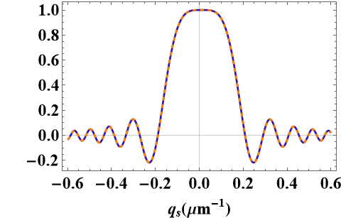
We analyze how the approximation we propose in Eq. (3)-(4) compares to the general phase matching function in Eq. (1) in Fig. 3. Assuming an idler photon wavelength of 800$\,\mathrm{nm}$, the double-sinc approximation (dashed orange curve) fits well the general phase matching function (solid blue curve) for a relatively large range of signal photon wavelengths LABEL:sub@fig:subfigaa, as long as the difference between signal and idler transverse momentum is not much bigger than $|q_{s}-q_{i}|\approx 0.02\,\mathrm{\mu m^{-1}}$. LABEL:sub@fig:subfigdd Similarly, the curves align nicely for a wide range of transverse momentum of the signal photon $q_{s}$ under the condition that the twin photons are wavelength degenerated. In summary, when the difference between the transverse momentum of the photons is small, there is a relatively loose restriction in the wavelength range allowed for the photons, and as long as the photons are of similar wavelength, approximately no limitation is applied to their transverse momentum. This reflects the PMF conditions under which the spatial and spectral degrees of freedom are decoupled.

Type-II SPDC

The SPDC type-II is characterized by associating orthogonal polarization to the signal and idler beams, with one of them having the same polarization as the pump beam. Consider that the pump beam propagates as an ordinary wave, and the signal and idler beams as ordinary and extraordinary waves ($o\rightarrow o+e$), respectively.

The wavevector mismatch for SPDC type-II is written as

$$\begin{split}\Delta k_{z}=&\bigg(\frac{1}{v_{g}^{p}}(\Omega_{s}+\Omega_{i})-\frac{1}{v_{g}^{s}}\Omega_{s}-\frac{1}{v_{g}^{i}}\Omega_{i}\bigg)\\ &+\frac{\text{GVD}_{p}}{2}(\Omega_{s}+\Omega_{i})^{2}-\frac{\text{GVD}_{s}}{2}\Omega_{s}^{2}-\frac{\text{GVD}_{i}}{2}\Omega_{i}^{2}\\ &-\frac{|\vec{q}_{s}|^{2}}{2k_{s}}-\frac{|\vec{q}_{i}|^{2}}{2k_{i}}.\end{split}$$ (16)

Assuming that the idler photon propagates along the principal axis of the crystal, we discard, without loss of generality, the spatial walk-off of the extraordinary beam ($\alpha=(\frac{\partial{k}}{\partial{\vec{q}}})=0$). Therefore, the spatial contribution for the phase mismatch for type-II is the same as for type-I Eq. (13).

$$\Delta k_{z}^{(\text{spatial})}\approx\frac{|\vec{q}_{s}-\vec{q}_{i}|^{2}}{2k_{p}}.$$ (17)

For the spectral contribution, we adopt here a strategy similar to that used for type-I SPDC, where we have dropped the pump temporal dispersion term $\frac{\text{GVD}_{p}}{2}(\Omega_{s}+\Omega_{i})^{2}$, keeping the linear term with the same dependence. The spectral counterpart of the mismatch for type-II reads as

$$\begin{split}\Delta k_{z}^{spec}\approx&-\frac{(\sqrt{\text{GVD}_{s}}\Omega_{s}-\sqrt{\text{GVD}_{i}}\Omega_{i})^{2}}{2}+\\ &+\frac{1}{v_{g}^{p}}(\Omega_{s}+\Omega_{i})-\frac{1}{v_{g}^{s}}\Omega_{s}-\frac{1}{v_{g}^{i}}\Omega_{i}\Bigg),\end{split}$$ (18)

where we have used the approximation

$$\mathrm{GVD}_{s}\Omega_{s}^{2}+\mathrm{GVD}_{i}\Omega_{i}^{2}\approx\tfrac{1}{2}(\sqrt{\mathrm{GVD}_{s}}\,\Omega_{s}-\sqrt{\mathrm{GVD}_{i}}\,\Omega_{i})^{2}.$$ (19)

Combining both spatial and spectral contributions yields the final approximated expression for the longitudinal phase mismatch of the SPDC type II:

$$\begin{split}\Delta k_{z}\approx&-\frac{|\vec{q}_{s}-\vec{q}_{i}|^{2}}{2k_{p}}+\frac{(\sqrt{\text{GVD}_{s}}\Omega_{s}-\sqrt{\text{GVD}_{i}}\Omega_{i})^{2}}{2}+\\ &-\frac{1}{v_{g}^{p}}(\Omega_{s}+\Omega_{i})+\frac{1}{v_{g}^{s}}\Omega_{s}+\frac{1}{v_{g}^{i}}\Omega_{i}.\end{split}$$ (20)

Appendix B Biphoton’s Gaussian Modelling

Type-I SPDC

We analyze in more detail how the spatial and spectral degrees of freedom contributes to the structure of the biphoton state, using the separable approximation in Eq. (4) for the phase-matching function Eq. (1).

Let us start by writing the two-photon wavefunction for a spectral and spatial Gaussian pump

$$\begin{split}\Phi(\vec{q_{s}},\vec{q_{i}},\Omega_{s},\Omega_{i})&=\Phi(\Omega_{s},\Omega_{i})\Phi(\vec{q_{s}},\vec{q_{i}}),\end{split}$$ (21)

where

$$\begin{split}\Phi(\vec{q_{s}},\vec{q_{i}})=&\mathrm{e}^{-w_{p}^{2}|\vec{q_{s}}+\vec{q_{i}}|^{2}}\operatorname{sinc}\left[\frac{L}{4k_{p}}|\vec{q_{s}}-\vec{q_{i}}|^{2}\right]\end{split}$$ (22)

and

$$\begin{split}&\Phi(\Omega_{s},\Omega_{i})=\exp\!\Bigl[-\tfrac{\tau^{2}}{8\ln 2}\,(\Omega_{s}+\Omega_{i})^{2}\Bigr]\;\\ &\times\operatorname{sinc}\!\Bigl[\tfrac{L}{2}\Bigl(\tfrac{\mathrm{GVD}_{s}}{4}\,(\Omega_{s}-\Omega_{i})^{2}-\bigl(\tfrac{1}{v_{g,p}}-\tfrac{1}{v_{g,s}}\bigr)\,(\Omega_{s}+\Omega_{i})\Bigr)\Bigr].\end{split}$$ (23)

The spatial phase matching function may be approximated by a Gaussian:

$$\operatorname{sinc}\bigg[\frac{L}{4k_{p}}(q_{x_{s}}-q_{x_{i}})^{2}\bigg]\approx\mathrm{exp}\bigg[-A\bigg(\frac{L}{4k_{p}}\bigg)(q_{x_{s}}-q_{x_{i}})^{2}\bigg],$$ (24)

Assuming that the argument of the sinc function matches that of the Gaussian, except for a constant prefactor $A=\frac{8}{3}$, which ensures that both functions yield the same second moments when integrated over the reduced probability density [21].

To model the spectral structure across arbitrary temporal pump profiles, we follow the framework developed by Fedorov and collaborators in Ref. [9]. For long pulses ($\Omega_{s}\approx-\Omega_{i}$), the sinc function can be well approximated by a Gaussian, and the joint spectral amplitude $\Phi(\Omega_{s},\Omega_{i})$ admits a direct double-Gaussian form. However, in the short-pulse regime, the coexistence of both linear and quadratic spectral terms in Eq. (23) leads to an asymmetric sinc function for which a direct Gaussian approximation is inaccurate. Instead, a Gaussian is fitted to the reduced spectral density instead $\rho_{s}(\Omega_{s},\Omega_{s}^{\prime})=\int d\Omega_{i}\,\Phi(\Omega_{s},\Omega_{i})\Phi^{*}(\Omega_{s}^{\prime},\Omega_{i})$, and by treating the asymptotic regimes and interpolating between them, a general double-Gaussian spectral wavefunction describes well the state for any pump pulse duration.

Under the approximations listed above, the spatially-spectrally separable wavefunction for type-I SPDC takes the four-Gaussian form

$$\begin{split}\Phi(x_{s},x_{i},\Omega_{s},\Omega_{i})=\mathcal{N}&\,\mathrm{e}^{-\frac{(x_{s}+x_{i})^{2}}{16w_{p}^{2}}}\,\mathrm{e}^{-\frac{(x_{s}-x_{i})^{2}}{16\sigma_{x}^{2}}}\\ &\times\mathrm{e}^{-\alpha\frac{(\Omega_{s}+\Omega_{i})^{2}}{2a^{2}(\tau)}}\,\mathrm{e}^{-\frac{(\Omega_{s}-\Omega_{i})^{2}}{2b^{2}(\tau)}},\end{split}$$ (25)

expressed in the transverse-position representation, obtained by inverse Fourier transforming the transverse-momentum counterpart in Eq. (7). $\mathcal{N}$, $w_{p}$ is the pump beam waist. The position correlation width parameter is defined as $\frac{1}{16\sigma_{x}^{2}}=\frac{3k_{p}}{8L}$. We set $\alpha=0.4$ for short pump pulses and $\alpha=1$ for long pump pulses, see Fig. 4(b) and (c).

The effective spectral widths are given by [9]

$$\begin{split}a(\tau)&=\frac{1.39}{\pi A\sqrt{\ln 2}}\frac{\lambda_{0}}{L}(1+\eta^{\gamma})^{-1/\gamma}\omega_{0},\\ \quad b(\tau)&=\sqrt{\frac{\lambda_{0}}{2\pi\cdot 0.249\cdot BL}}\cdot\frac{(1+\eta^{\gamma})^{1/2\gamma}\omega_{0}}{\sqrt{\eta}},\end{split}$$ (26)

where the auxiliary parameters are defined as follows:

$$\begin{split}A&=\left(\frac{1}{v_{g,p}}-\frac{1}{v_{g,s}}\right)^{-1},\quad\eta=\frac{2c\tau}{AL},\quad\\ B&=\frac{\omega_{0}c\,\mathrm{GVD}_{s}}{4},\quad\gamma=2.21.\end{split}$$ (27)

Recall that $\omega_{0}$ denote the central frequency of the pump spectrum, $c$ is the speed of light, $\tau$ is the pump pulse duration and $L$ is the crystal length.

To investigate whether our four-Gaussian model, while analytically simple but not simplistic, accurately captures the decoupled spatial-spectral structure of the general biphoton wavefunction, we compare it with the general model under representative experimental conditions. Figure 4 illustrates the squared modulus of the type I SPDC general wavefunction (solid blue curve), given by a spatial-spectral Gaussian pump functions and the PMF Eq. (2)-(1), and the approximation (dashed orange curve) given by the four-Gaussian introduced in Eq. (7).

Panel Fig. 4LABEL:sub@fig:subfigag shows the spatial profile of the biphoton amplitude as a function of the signal photon’s transverse position $x_{s}$, with the idler fixed at $x_{i}=1\,\mu\mathrm{m}$ and both photons at the wavelength $\lambda_{s}=\lambda_{i}=800\,\mathrm{nm}$. Notice that, within the conditions we set, the probability density obtained from the four-Gaussian wavefunction fairly agrees with the one from the general wavefunction over a wide spatial range. We observed the same spatial profiles for $\tau=50\,\mathrm{ps}$ and $\tau=50\,\mathrm{fs}$, that is why we show only one case here. This result is consistent with the fact that the pump pulse duration should not affect the spatial component of the state in a regime where the two degrees of freedom are decoupled.

A long pump pulse yields a narrow spectral bandwidth, while a short pulse allows a much broader signal and idler wavelength combination. LABEL:sub@fig:subfigbg In the spectral domain, we note a relatively good agreement between the curves if the photons are perfectly indistinguishable in wavelength for a long pump pulse duration ($\tau=50\,\mathrm{ps}$), and photon’s separation of $2\,\mathrm{\mu m}$. LABEL:sub@fig:subfigcg For a short pump pulse duration ($\tau=50\,\mathrm{fs}$), the spatial and spectral degrees of freedom remain decoupled even for a certain bandwidth, our model covers this behavior by adjusting the parameter $\alpha$ in Eq. (7).

(a)

(b)

(c)

Fig. 4: The squared modulus of the SPDC type-I general wavefunction Eq. (2)-(1) (solid blue curve) and of its four-Gaussian approximation Eq. (7) (dashed orange curve). LABEL:sub@fig:subfigag When plotted as a function of the signal position, the four-Gaussian gives a reasonable estimate of the general wavefunction for photons with the same wavelength without discriminating a specific photon’s position. The general wavefunction requires wavelength degenerated photons when the pump pulse duration is long LABEL:sub@fig:subfigbg, and allows a certain bandwidth for shorter pump pulse duration LABEL:sub@fig:subfigcg. Plots obtained for a SPDC type-I photons exiting a $L=0.5\,\mathrm{mm}$ LiIO3 crystal, pump wavelength $\lambda_{p}=400\,\mathrm{nm}$ and beam waist $w_{p}=28\,\mathrm{\mu m}$, .

Type-II SPDC

Defining the general wavefunction for the SPDC type II as

$$\begin{split}\Phi_{\text{II}}=&\mathrm{e}^{-w_{p}^{2}|\vec{q_{s}}+\vec{q_{i}}|^{2}}\mathrm{e}^{-{\frac{\tau^{2}}{8\ln{2}}(\Omega_{s}+\Omega_{i})^{2}}}\operatorname{sinc}\left[\frac{\Delta k_{z}L}{2}\right],\end{split}$$ (28)

and building upon the approach used for type-I SPDC, we now construct an approximate form of the biphoton wavefunction for type-II SPDC. Starting from the separable spatial and spectral phase-matching components

$$\begin{split}\Phi_{\text{II}}\approx&\mathrm{e}^{-w_{p}^{2}|\vec{q_{s}}+\vec{q_{i}}|^{2}}\mathrm{e}^{-{\frac{\tau^{2}}{8\ln{2}}(\Omega_{s}+\Omega_{i})^{2}}}\Theta(q_{s},q_{i})\tilde{\Theta}(\Omega_{s},\Omega_{i}),\end{split}$$ (29)

with

$$\begin{split}\Theta(\vec{q_{s}},\vec{q_{i}})=&\mathrm{e}^{-w_{p}^{2}|\vec{q_{s}}+\vec{q_{i}}|^{2}}\operatorname{sinc}\left[\frac{L}{4k_{p}}|\vec{q_{s}}-\vec{q_{i}}|^{2}\right],\end{split}$$ (30)

and

$$\begin{split}\tilde{\Theta}(\Omega_{s},\Omega_{i})=\operatorname{sinc}\!\Biggl[\frac{L}{2}\Biggl(&-\frac{(\sqrt{\text{GVD}_{s}}\Omega_{s}-\sqrt{\text{GVD}_{i}}\Omega_{i})^{2}}{2}\\ &+\frac{1}{v_{g}^{p}}(\Omega_{s}+\Omega_{i})-\frac{1}{v_{g}^{s}}\Omega_{s}-\frac{1}{v_{g}^{i}}\Omega_{i}\Biggr)\Biggr].\end{split}$$ (31)

$$\begin{split}\psi(x_{s},x_{i},\Omega_{s},\Omega_{i})=&\,\mathrm{e}^{-\frac{(x_{s}+x_{i})^{2}}{16w_{p}^{2}}}\,\mathrm{e}^{-\frac{(x_{s}-x_{i})^{2}}{16\sigma_{x}^{2}}}\\ &\times\mathrm{e}^{-\beta\frac{(\Omega_{s}+\Omega_{i})^{2}}{2a^{2}(\tau)}}\,\mathrm{e}^{-\frac{(\sqrt{\mathrm{GVD}_{s}}\Omega_{s}-\sqrt{\mathrm{GVD}_{i}}\Omega_{i})^{2}}{2b^{2}(\tau)}}.\end{split}$$ (32)

Where we adjust the parameter $\beta$ according to the pump pulse duration $\beta=1$ for long pulses and $\beta=0.1$ for short pulses, ensuring that the this approximation closely matches the general wavefunction across regimes.

The asymmetry in dispersion (arising from the phase-matching configuration in type-II SPDC, where signal and idler photons are orthogonally polarized propagating differently in a birefringent medium) plays a central role in shaping the joint spectral amplitude. Our four-Gaussian model captures this effect by explicitly incorporating distinct GVD terms for the signal and idler into the spectral Gaussian that represents the phase-matching function. This level of control offers a tunable framework for tailoring group-velocity conditions in high-purity photon applications, such as heralded single-photon sources and quantum-interference schemes.

For wavelength-degenerate photons, the pump pulse durations will not affect the spatial profile of the photons, as we are using parameters describing a region where the two degrees of freedom are decoupled. Since the resulting behavior mirrors what is shown in Fig. 4LABEL:sub@fig:subfigag for type-I, we do not repeat it here. Compared to the type-I case, the main difference in the approximate model lies in the spectral profile, due to the asymmetric GVD contributions in type-II.

(a)

(b)

Fig. 5: Squared modulus of the general type-II wavefunction Eq. (28)-(20) (solid blue curve) with its four-Gaussian approximation  Eq. (32) (dashed orange curve) as a function of the signal wavelength. Different pump pulse regimes are analyzed, long ($\tau=50\,\mathrm{ps}$) LABEL:sub@fig:subfigbII and short pulse duration ($\tau=50\,\mathrm{fs}$) LABEL:sub@fig:subfigcII. As in the type-I case, a longer pulse constrains the spectral bandwidth of the twin-photons, while a shorter pulse broadens it. The type-II spectrum is slightly wider than type-I, a feature well captured by the four-Gaussian approximation with the proper $\beta$ adjustment. For photons generated from a $L=0.5\,\mathrm{mm}$ BBO crystal with pump wavelength $\lambda_{p}=400\,\mathrm{nm}$, beam waist $w_{p}=28\,\mathrm{\mu m}$, group velocities $v_{g,p}=c/1.708$, $v_{g,s}=c/1.626$ and $v_{g,i}=c/1.684$, group velocity dispersion $\text{GVD}_{p}=180\,\mathrm{fs}^{2}/\,\mathrm{mm}$, $\text{GVD}_{s}=61.7\,\mathrm{fs}^{2}/\,\mathrm{mm}$ and $\text{GVD}_{p}=75.1\,\mathrm{fs}^{2}/\,\mathrm{mm}$.

In Fig. 5, we compare the squared modulus of the general type-II wavefunction Eq. (28)-(20) (solid blue curve) with its four-Gaussian approximation  Eq. (32) (dashed orange curve) as a function of the signal wavelength. Panels LABEL:sub@fig:subfigbII and LABEL:sub@fig:subfigcII illustrate the cases of long ($\tau=50\,\mathrm{ps}$) and short ($\tau=50\,\mathrm{fs}$) pump pulses, respectively. We confirm the same behavior obtained for type I: a long pump pulse yields a narrow spectral bandwidth, and a wider bandwidth for short pulse. Additionally, we note that the spectral bandwidth for type-II is slightly broader than for type-I. This broader spectrum is well reproduced by the approximation with an appropriate choice of $\beta$ in Eq. (32).

(a)

(b)

(c)

Fig. 6: Joint spectral amplitude (JSA) profiles generated using the proposed four-Gaussian model for type-II SPDC, which explicitly incorporates the asymmetry in signal and idler group velocity dispersion (GVD) into the phase-matching function. The resulting JSA is shaped by the interplay between the pump envelope (constraining the frequency sum) and the GVD-weighted phase matching (constraining the frequency difference). (a) and (c) For GVD_s-GVD_i equal to 1.34 and -1, the JSA becomes elongated and tilted, forming an elliptical distribution. (b) For GVD_s-GVD_i = 0.66, the JSA is nearly circular, reflecting a more symmetric spectral constraint. These results illustrate how the GVD asymmetry in the type-II model governs the orientation and ellipticity of spectral correlations.

As shown in the overlaid plots in Fig. 6, for intermediate pump durations (neither ultrashort nor continuous-wave), the relative orientation and ellipticity of the JSA are governed by the asymmetry between signal and idler GVD coefficients. In panels (a) and (c), the JSA is visibly elliptical, with a longer axis tilted toward the signal or idler frequency with a stronger dispersion experienced (signal-(a) and idler-(c)). In contrast, in the second plot ($\text{GVD}_{s}=1$, $\text{GVD}_{s}=0.34$), the reduced dispersion causes the JSA to become nearly circular, reflecting a more symmetric phase-matching constraint.

References

- [1] (2002) Quantum-optical coherence tomography with dispersion cancellation. Physical Review A 65 (5), pp. 053817. Cited by: §I, §IV.
- [2] (2005) Generation of hyperentangled photon pairs. Physical review letters 95 (26), pp. 260501. Cited by: §I.
- [3] (2010) Spatiotemporal structure of biphoton entanglement in type-ii parametric down-conversion. Physical Review A 82 (1), pp. 013835. Cited by: §I.
- [4] (2018) Distribution of high-dimensional orbital angular momentum entanglement at telecom wavelength over 1km of optical fibre. arXiv preprint arXiv:1811.12195. Cited by: §I, §IV.
- [5] (2010) Tailoring the spatiotemporal structure of biphoton entanglement in type-i parametric down-conversion. Physical Review A 81 (3), pp. 033808. Cited by: §I.
- [6] (2021) Biphoton phase-space correlations from gouy-phase measurements using double slits. Physical Review A 104 (6), pp. 062430. Cited by: §II.
- [7] (2021) Gouy phase of type-i spdc-generated biphotons. Physics Letters A 386, pp. 126989. Cited by: §II.
- [8] (2019) Overcoming noise in entanglement distribution. Physical Review X 9 (4), pp. 041042. Cited by: §I, §IV.
- [9] (2009) Gaussian modelling and schmidt modes of spdc biphoton states. Journal of Physics B: Atomic, Molecular and Optical Physics 42 (17), pp. 175503. Cited by: Appendix A, Appendix B, Appendix B, §II.0.1, §II.
- [10] (2005) Spiral phase contrast imaging in microscopy. Optics Express 13 (3), pp. 689–694. Cited by: §IV.
- [11] (2009) X entanglement: the nonfactorable spatiotemporal structure of biphoton correlation. Physical review letters 102 (22), pp. 223601. Cited by: §I.
- [12] (2001) Eliminating frequency and space-time correlations in multiphoton states. Physical Review A 64 (6), pp. 063815. Cited by: §I.
- [13] (2006) Experimental quantum cryptography with qutrits. New Journal of Physics 8 (5), pp. 75. Cited by: §I.
- [14] (2009) Modeling and optimization of photon pair sources based on spontaneous parametric down-conversion. Physical Review A—Atomic, Molecular, and Optical Physics 80 (1), pp. 013811. Cited by: §II.
- [15] (2024) Phase preservation of orbital angular momentum of light in multiple scattering environment. Light: Science & Applications 13 (1), pp. 214. Cited by: §IV.
- [16] (2008) Biphoton wave packets in parametric down-conversion: spectral and temporal structure and degree of entanglement. Physical Review A—Atomic, Molecular, and Optical Physics 78 (6), pp. 062327. Cited by: Fig. 1, §II.
- [17] (2017) Remotely sensing an object’s rotational orientation using the orbital angular momentum of light. Chinese Optics Letters 15 (3), pp. 030012. Cited by: §IV.
- [18] (2015) High-dimensional quantum cryptography with twisted light. New Journal of Physics 17 (3), pp. 033033. Cited by: §I.
- [19] (2008) Spatiotemporal correlations in entangled photons generated by spontaneous parametric down conversion. New Journal of Physics 10 (11), pp. 113012. Cited by: §I.
- [20] (2017) Quality of spatial entanglement propagation. Physical Review A 95 (6), pp. 063836. Cited by: §II.
- [21] (2016) Introduction to the transverse spatial correlations in spontaneous parametric down-conversion through the biphoton birth zone. Journal of Optics 18 (5), pp. 053501. Cited by: Appendix A, Appendix B, §II, §II.
- [22] (2003) Quantum information processing and precise optical measurement with entangled-photon pairs. Contemporary Physics 44 (4), pp. 341–356. Cited by: §I.
- [23] (2007) Shaping the waveform of entangled photons. Physical review letters 99 (24), pp. 243601. Cited by: §I, Fig. 1.
- [24] (2020) Optimizing spontaneous parametric down-conversion sources for boson sampling. Physical Review A 101 (6), pp. 063821. Cited by: §I.
- [25] (2015) Gradual edge enhancement in spiral phase contrast imaging with fractional vortex filters. Scientific Reports 5 (1), pp. 15826. Cited by: §I, §IV, §IV.
- [26] (2021) Generating heralded single photons with a switchable orbital angular momentum mode. Photonics Research 9 (9), pp. 1865–1870. Cited by: §IV.
- [27] (2017) Simultaneous entanglement swapping of multiple orbital angular momentum states of light. Nature communications 8 (1), pp. 632. Cited by: §IV.