Dictionary Based Pattern Entropy for Causal Direction Discovery

Abstract

Discovering causal direction from temporal observational data is particularly challenging for symbolic sequences, where functional models and noise assumptions are often unavailable. We propose a novel Dictionary Based Pattern Entropy ($DPE$) framework that infers both the direction of causation and the specific subpatterns driving changes in the effect variable. The framework integrates Algorithmic Information Theory (AIT) and Shannon Information Theory. Causation is interpreted as the emergence of compact, rule based patterns in the candidate cause that systematically constrain the effect. $DPE$ constructs direction-specific dictionaries and quantifies their influence using entropy-based measures, enabling a principled link between deterministic pattern structure and stochastic variability. Causal direction is inferred via a minimum-uncertainty criterion, selecting the direction exhibiting stronger and more consistent pattern-driven organization. As summarized in Table 7, $DPE$ consistently achieves reliable performance across diverse synthetic systems, including delayed bit-flip perturbations, AR(1) coupling, 1D skew-tent maps, and sparse processes, outperforming or matching competing AIT-based methods ($ETC_{E}$, $ETC_{P}$, $LZ_{P}$). In biological and ecological datasets, performance is competitive, while alternative methods show advantages in specific genomic settings. Overall, the results demonstrate that minimizing pattern level uncertainty yields a robust, interpretable, and broadly applicable framework for causal discovery.

1 Introduction

Modern artificial intelligence systems, particularly state of the art machine learning models, are primarily designed to estimate a functional mapping $f:\mathcal{X}\rightarrow\mathcal{Y}$ from input features to target outcomes using empirical data. These models are optimized to capture statistical regularities and associations that maximize predictive performance. However, such associations do not, in general, imply causal relationships. A learned functional dependence between variables does not establish whether a given feature exerts a causal influence on the outcome or merely correlates with it due to confounding or latent factors.

Identifying causal relationships typically requires intervention. In the standard causal inference framework, interventional queries are formalized through the $do(\cdot)$ operator. Specifically, the causal effect of $X$ on $Y$ is characterized by comparing the interventional distribution $P(Y\mid do(X=x))$ across different values of $x$. The Randomized Controlled Trial (RCT) is widely regarded as the gold standard for establishing causal effects because randomization mitigates confounding by ensuring statistical independence between treatment assignment and potential outcomes. Nevertheless, in many domains, conducting an RCT is either technically infeasible, economically impractical, or ethically impermissible. For instance, assigning individuals to smoke in order to test its effect on cancer incidence would violate fundamental ethical principles. In such settings, researchers must rely on observational data, such as historical records comparing smokers and non-smokers, to infer causal relationships.

Causal discovery from observational data aims to recover aspects of the underlying causal structure without controlled interventions. The methods used in causal discovery from observational data can be broadly classified into the following categories:

• Graph Based (Constraint & Score Based) Spirtes et al. [2000], Chickering [2002]

• Functional Causal Models (FCMs) Shimizu et al. [2006], Hoyer et al. [2008]

• Algorithmic Information Theory (AIT) Budhathoki and Vreeken [2016]

• Information Theoretic (Shannon-Based) Schreiber [2000]

• Temporal & Predictive (Time Series) Granger [1969]

• Dynamical Systems (State Space) Sugihara et al. [2012]

Graph-based approaches Neuberg [2003], rooted in structural causal models (SCMs), aim to recover causal structure by exploiting conditional independence relationships (constraint-based methods) or by optimizing global model scores over the space of possible graphs (score-based methods). Closely related but conceptually distinct are functional causal models (FCMs) Shimizu et al. [2006], Hoyer et al. [2008], which identify causal direction by leveraging asymmetries in the data-generating process, such as independence between causes and noise in additive noise models or assumptions of non-Gaussianity in linear models. Both types of methods typically seek to reconstruct causal graphs or directed relationships under explicit modeling assumptions, though the assumptions and identifiability conditions differ between approaches.

In contrast, several frameworks infer causal direction without explicitly specifying structural equations. Algorithmic information-theoretic approaches build on Kolmogorov complexity Dhruthi et al. [2025], Xu et al. [2025], Wendong et al. [2025] and the Algorithmic Markov Condition Janzing and Schölkopf [2010], asserting that the true causal direction yields a shorter description of the joint distribution than the reverse Budhathoki and Vreeken [2016]. Operationally, this principle is instantiated through Minimum Description Length (MDL) formulations Grünwald [2007] and compression-based complexity measures.

Representative methods include ORIGO, which infers causal direction by minimizing regression-based description length Budhathoki and Vreeken [2016]; ERGO, an entropy-based regression framework grounded in MDL principles Vreeken [2015]; and Compression Complexity Causality (CCC), which leverages Effort-To-Compress (ETC) to quantify directed influence in time series Kathpalia and Nagaraj [2019]. Related approaches employ Lempel–Ziv complexity and grammar-based compression measures to detect asymmetry via differential compressibility rather than explicit functional modeling Sy and Nagaraj [2021]. Collectively, these methods attribute causality to the direction that admits a more parsimonious description of the data.

Information theoretic methods quantify directed statistical dependencies or directed information flow Schreiber [2000], while temporal and predictive frameworks, such as Granger causality Granger [1969], infer causation from asymmetric predictability in time-ordered observations. Finally, dynamical systems approaches, including state space reconstruction and convergent cross mapping Sugihara et al. [2012], exploit properties of coupled nonlinear systems to detect causal influence from reconstructed dynamics. Together, these approaches highlight that causal discovery from observational data is not governed by a single unifying framework, but instead reflects multiple complementary perspectives on causal inference.

Despite their diversity, all approaches to causal discovery from observational data rely on assumptions that constrain identifiability. Graphical and functional models impose assumptions on conditional independence, functional form, or noise structure, while compression based and information theoretic approaches depend on approximations to algorithmic complexity or information flow. In particular, information theoretic measures require accurate probability estimation for entropy and related quantities Nagaraj [2021], which typically necessitates long sequences or large sample sizes. In data-scarce or highly structured observational settings, such global estimates can become unreliable, limiting their practical applicability.

In this work, we propose a methodology that combines Algorithmic Information Theory (AIT) and Shannon’s Information Theory (IT) to perform causal discovery from noisy observational data.

• Algorithmic Perspective: Inspired by AIT, we treat causal relationships as “governing programs” rather than statistical correlations. The method extracts a dictionary of recurring sub-patterns, which represent latent mechanistic units driving the effect. In essence, we aim to find the most compact, pattern based description of how variables influence or trigger each other.

• Information-Theoretic Validation: To account for noise in real data, we use Shannon entropy to measure the reliability of the extracted dictionary. Our metric, Response Determinism ($R$-flip), quantifies how strongly a sub-pattern in $X$ predicts a change in $Y$, with values ranging from 0 (no change) to 1 (definite change). Both $0$ and $1$, indicates determinism.

Overall, the framework reveals deterministic causal structure in the data: influence values of $0$ or $1$ correspond to fully deterministic effects, implying zero entropy (no surprise or uncertainty) in the induced response. Intermediate values indicate residual uncertainty, reflecting stochastic components in the relationship. Lower uncertainty (or reduced surprise) in the direction signaling stronger deterministic influence relative to the reverse direction.

The remainder of the paper is organized as follows. Section 2 presents the proposed methodology, illustrated with a worked example. Section 3 describes the experimental setup and compares the performance of the proposed approach with other AIT-based causal discovery algorithms. Section 4 discusses the results and their implications. Section 5 outlines the limitations of the current framework and directions for future work. Finally, Section 6 concludes the paper.

2 Methodology

In this section, we provide a detailed explanation of the proposed method Dictionary Based Pattern Entropy for causal discovery from two variables.

2.1 Dictionary Based Pattern Entropy (DPE)

Let $X=(x_{1},x_{2},\ldots,x_{N})$, $Y=(y_{1},y_{2},\ldots,y_{N})$ denote two symbolic sequences of equal length $N$, where each symbol $x_{i}$ and $y_{i}$ takes values from a finite alphabet $\mathcal{A}$ (e.g., $\mathcal{A}=\{0,1\}$ for binary sequences). The objective of this work is to infer causal relationships between $X$ and $Y$ directly from their observed symbolic patterns, without assuming explicit probabilistic models, functional forms, or long sequence asymptotics.

We introduce a causal inference framework termed Dictionary Based Pattern Entropy ($DPE$), which leverages dictionary construction and pattern sensitive information measures to characterize causal asymmetries between symbolic sequences. The goals of the proposed $DPE$ framework are twofold:

1. To determine the direction of causality between $X$ and $Y$ by identifying asymmetric pattern driven information changes, i.e., whether variations in $X$ induce structured changes in $Y$ or vice versa.

2. To identify and attribute causal influence to specific patterns within the inferred causal sequence that are responsible for observable symbolic transitions in the effect sequence, thereby enabling pattern level attribution of causal strength.

This section highlights the proposed method and a worked out example to understand the method developed to solve the problems mentioned under section 2.1.

2.1.1 Causal Direction Identification

We say that $X$ is causal for $Y$ if recurring finite patterns in $X$ systematically determine the transition behavior of $Y$. Under this definition, causal directionality reduces to identifying finite patterns in one sequence whose occurrences deterministically fix the transition behavior of the other. The following steps operationalize this principle to determine the causal direction between two variables, $X$ and $Y$. A worked example is provided for illustration.

Let the input sequence be a binary string $X=(x_{1},x_{2},\dots,x_{n})$, $x_{i}\in\{0,1\}$. The corresponding output sequence is denoted as $Y=(y_{1},y_{2},\dots,y_{n})$, $y_{i}\in\{0,1\}$. The sequence $Y$ is constructed to reflect the occurrence of the pattern 1101 within $X$, allowing overlapping instances. That is, whenever the subsequence 1101 appears in $X$, a symbolic transition is induced in $Y$ at the corresponding position. Formally, the output is defined as

$$y_{i}=\begin{cases}1,&\text{if }(x_{i-3},x_{i-2},x_{i-1},x_{i})=(1,1,0,1),\\[6.0pt] 0,&\text{otherwise.}\end{cases}$$

Hence, the output $Y$ takes the value $1$ whenever the input sequence $X$ contains the subsequence 1101, even if such occurrences overlap; otherwise, the output remains $0$. Consider the following symbolic sequences:

$$X=011101111010011001110101101001$$

The pattern set is defined as:

$$\text{Patterns}=\{1101\}$$

The corresponding output sequence is:

$$Y=000001000010000000000100001000$$

1. Step 1: Initialization. We define a dictionary that stores the segments (or patterns) of $X$ corresponding to the points where a change occurs in $Y$ as $G_{X\rightarrow Y}$. Similarly, we define $G_{Y\rightarrow X}$ as the dictionary that stores the segments of $Y$ whenever a change occurs in $X$. Initially, both dictionaries are empty:

   $$G_{X\rightarrow Y}=G_{Y\rightarrow X}=\{\}.$$

2. Step 2: Construction of $G_{X\rightarrow Y}$

   A bit flip in $Y$ is said to occur at position $k>1$ if

   $$y_{k}\neq y_{k-1}.$$

   The dictionary $G_{X\rightarrow Y}$ is constructed by scanning $Y$ from left to right. Let $s$ denote the current starting index, initialized as $s=1$.

   Whenever a bit flip occurs at position $k$, we extract the substring

   $$(x_{s},x_{s+1},\dots,x_{k})$$

   of $X$, which explicitly includes the symbol $x_{k}$ aligned with the flip in $Y$. This substring is inserted into $G_{X\rightarrow Y}$. The starting index is then updated to $s=k+1$, and the scan continues until the next bit flip in $Y$. Repeated substrings are stored only once in the dictionary.

   For the illustrative example below, consider:

   $$Y=000001000010000000000100001000,$$

   $$X=011101111010011001110101101001.$$

   We highlight in red the sub-pattern in $Y$ where a bit flip occurs, and the corresponding sub-pattern in $X$ recorded into $G_{X\rightarrow Y}$.

   First bit flip in $Y$:

   $Y=\text{ \hbox to34.5pt{\vbox to6.44pt{\pgfpicture\makeatletter\hbox{\qquad\lower 0.0pt\hbox to0.0pt{\pgfsys@beginscope\pgfsys@invoke{ }\definecolor{pgfstrokecolor}{rgb}{0,0,0}\pgfsys@color@rgb@stroke{0}{0}{0}\pgfsys@invoke{ }\pgfsys@color@rgb@fill{0}{0}{0}\pgfsys@invoke{ }\pgfsys@setlinewidth{\the\pgflinewidth}\pgfsys@invoke{ }\nullfont\pgfsys@beginscope\pgfsys@invoke{ }\pgfsys@invoke{ }\pgfsys@endscope\hbox to0.0pt{\pgfsys@beginscope\pgfsys@invoke{ }{}{ {{}}\hbox{\hbox{{\pgfsys@beginscope\pgfsys@invoke{ }{{}{}{{ {}{}}}{ {}{}} {{}{{}}}{{}{}}{}{{}{}} { }{{{{}}\pgfsys@beginscope\pgfsys@invoke{ }\pgfsys@transformcm{1.0}{0.0}{0.0}{1.0}{-17.24991pt}{0.0pt}\pgfsys@invoke{ }\hbox{{\definecolor{pgfstrokecolor}{rgb}{0,0,0}\pgfsys@color@rgb@stroke{0}{0}{0}\pgfsys@invoke{ }\pgfsys@color@rgb@fill{0}{0}{0}\pgfsys@invoke{ }\hbox{{{000001}}} }}\pgfsys@invoke{ }\pgfsys@endscope}}} \pgfsys@invoke{ }\pgfsys@endscope}}} } \pgfsys@invoke{ }\pgfsys@endscope\hbox to0.0pt{}{{ {}{}{}}}{}{}\hss}\pgfsys@discardpath\pgfsys@invoke{ }\pgfsys@endscope\hss}}\endpgfpicture}} 000010000000000100001000 }$

   $X=\text{ \hbox to34.5pt{\vbox to6.44pt{\pgfpicture\makeatletter\hbox{\qquad\lower 0.0pt\hbox to0.0pt{\pgfsys@beginscope\pgfsys@invoke{ }\definecolor{pgfstrokecolor}{rgb}{0,0,0}\pgfsys@color@rgb@stroke{0}{0}{0}\pgfsys@invoke{ }\pgfsys@color@rgb@fill{0}{0}{0}\pgfsys@invoke{ }\pgfsys@setlinewidth{\the\pgflinewidth}\pgfsys@invoke{ }\nullfont\pgfsys@beginscope\pgfsys@invoke{ }\pgfsys@invoke{ }\pgfsys@endscope\hbox to0.0pt{\pgfsys@beginscope\pgfsys@invoke{ }{}{ {{}}\hbox{\hbox{{\pgfsys@beginscope\pgfsys@invoke{ }{{}{}{{ {}{}}}{ {}{}} {{}{{}}}{{}{}}{}{{}{}} { }{{{{}}\pgfsys@beginscope\pgfsys@invoke{ }\pgfsys@transformcm{1.0}{0.0}{0.0}{1.0}{-17.24991pt}{0.0pt}\pgfsys@invoke{ }\hbox{{\definecolor{pgfstrokecolor}{rgb}{0,0,0}\pgfsys@color@rgb@stroke{0}{0}{0}\pgfsys@invoke{ }\pgfsys@color@rgb@fill{0}{0}{0}\pgfsys@invoke{ }\hbox{{{011101}}} }}\pgfsys@invoke{ }\pgfsys@endscope}}} \pgfsys@invoke{ }\pgfsys@endscope}}} } \pgfsys@invoke{ }\pgfsys@endscope\hbox to0.0pt{}{{ {}{}{}}}{}{}\hss}\pgfsys@discardpath\pgfsys@invoke{ }\pgfsys@endscope\hss}}\endpgfpicture}} 111010011001110101101001 }$

   Hence, $G_{X\rightarrow Y}=\{011101\}$.

   Second bit flip in $Y$:

   $Y=\text{ 000001 \hbox to28.75pt{\vbox to6.44pt{\pgfpicture\makeatletter\hbox{\qquad\lower 0.0pt\hbox to0.0pt{\pgfsys@beginscope\pgfsys@invoke{ }\definecolor{pgfstrokecolor}{rgb}{0,0,0}\pgfsys@color@rgb@stroke{0}{0}{0}\pgfsys@invoke{ }\pgfsys@color@rgb@fill{0}{0}{0}\pgfsys@invoke{ }\pgfsys@setlinewidth{\the\pgflinewidth}\pgfsys@invoke{ }\nullfont\pgfsys@beginscope\pgfsys@invoke{ }\pgfsys@invoke{ }\pgfsys@endscope\hbox to0.0pt{\pgfsys@beginscope\pgfsys@invoke{ }{}{ {{}}\hbox{\hbox{{\pgfsys@beginscope\pgfsys@invoke{ }{{}{}{{ {}{}}}{ {}{}} {{}{{}}}{{}{}}{}{{}{}} { }{{{{}}\pgfsys@beginscope\pgfsys@invoke{ }\pgfsys@transformcm{1.0}{0.0}{0.0}{1.0}{-14.37492pt}{0.0pt}\pgfsys@invoke{ }\hbox{{\definecolor{pgfstrokecolor}{rgb}{0,0,0}\pgfsys@color@rgb@stroke{0}{0}{0}\pgfsys@invoke{ }\pgfsys@color@rgb@fill{0}{0}{0}\pgfsys@invoke{ }\hbox{{{00001}}} }}\pgfsys@invoke{ }\pgfsys@endscope}}} \pgfsys@invoke{ }\pgfsys@endscope}}} } \pgfsys@invoke{ }\pgfsys@endscope\hbox to0.0pt{}{{ {}{}{}}}{}{}\hss}\pgfsys@discardpath\pgfsys@invoke{ }\pgfsys@endscope\hss}}\endpgfpicture}} 0000000000100001000 }$

   $X=\text{ 011101 \hbox to28.75pt{\vbox to6.44pt{\pgfpicture\makeatletter\hbox{\qquad\lower 0.0pt\hbox to0.0pt{\pgfsys@beginscope\pgfsys@invoke{ }\definecolor{pgfstrokecolor}{rgb}{0,0,0}\pgfsys@color@rgb@stroke{0}{0}{0}\pgfsys@invoke{ }\pgfsys@color@rgb@fill{0}{0}{0}\pgfsys@invoke{ }\pgfsys@setlinewidth{\the\pgflinewidth}\pgfsys@invoke{ }\nullfont\pgfsys@beginscope\pgfsys@invoke{ }\pgfsys@invoke{ }\pgfsys@endscope\hbox to0.0pt{\pgfsys@beginscope\pgfsys@invoke{ }{}{ {{}}\hbox{\hbox{{\pgfsys@beginscope\pgfsys@invoke{ }{{}{}{{ {}{}}}{ {}{}} {{}{{}}}{{}{}}{}{{}{}} { }{{{{}}\pgfsys@beginscope\pgfsys@invoke{ }\pgfsys@transformcm{1.0}{0.0}{0.0}{1.0}{-14.37492pt}{0.0pt}\pgfsys@invoke{ }\hbox{{\definecolor{pgfstrokecolor}{rgb}{0,0,0}\pgfsys@color@rgb@stroke{0}{0}{0}\pgfsys@invoke{ }\pgfsys@color@rgb@fill{0}{0}{0}\pgfsys@invoke{ }\hbox{{{11101}}} }}\pgfsys@invoke{ }\pgfsys@endscope}}} \pgfsys@invoke{ }\pgfsys@endscope}}} } \pgfsys@invoke{ }\pgfsys@endscope\hbox to0.0pt{}{{ {}{}{}}}{}{}\hss}\pgfsys@discardpath\pgfsys@invoke{ }\pgfsys@endscope\hss}}\endpgfpicture}} 0011001110101101001 }$

   Now, $G_{X\rightarrow Y}=\{011101,\,11101\}$.

   Third bit flip in $Y$:

   $Y=\text{ 00000100001 \hbox to63.25pt{\vbox to6.44pt{\pgfpicture\makeatletter\hbox{\hskip 31.62483pt\lower 0.0pt\hbox to0.0pt{\pgfsys@beginscope\pgfsys@invoke{ }\definecolor{pgfstrokecolor}{rgb}{0,0,0}\pgfsys@color@rgb@stroke{0}{0}{0}\pgfsys@invoke{ }\pgfsys@color@rgb@fill{0}{0}{0}\pgfsys@invoke{ }\pgfsys@setlinewidth{\the\pgflinewidth}\pgfsys@invoke{ }\nullfont\pgfsys@beginscope\pgfsys@invoke{ }\pgfsys@invoke{ }\pgfsys@endscope\hbox to0.0pt{\pgfsys@beginscope\pgfsys@invoke{ }{}{ {{}}\hbox{\hbox{{\pgfsys@beginscope\pgfsys@invoke{ }{{}{}{{ {}{}}}{ {}{}} {{}{{}}}{{}{}}{}{{}{}} { }{{{{}}\pgfsys@beginscope\pgfsys@invoke{ }\pgfsys@transformcm{1.0}{0.0}{0.0}{1.0}{-31.62483pt}{0.0pt}\pgfsys@invoke{ }\hbox{{\definecolor{pgfstrokecolor}{rgb}{0,0,0}\pgfsys@color@rgb@stroke{0}{0}{0}\pgfsys@invoke{ }\pgfsys@color@rgb@fill{0}{0}{0}\pgfsys@invoke{ }\hbox{{{00000000001}}} }}\pgfsys@invoke{ }\pgfsys@endscope}}} \pgfsys@invoke{ }\pgfsys@endscope}}} } \pgfsys@invoke{ }\pgfsys@endscope\hbox to0.0pt{}{{ {}{}{}}}{}{}\hss}\pgfsys@discardpath\pgfsys@invoke{ }\pgfsys@endscope\hss}}\endpgfpicture}} 00001000 }$

   $X=\text{ 01110111101 \hbox to63.25pt{\vbox to6.44pt{\pgfpicture\makeatletter\hbox{\hskip 31.62483pt\lower 0.0pt\hbox to0.0pt{\pgfsys@beginscope\pgfsys@invoke{ }\definecolor{pgfstrokecolor}{rgb}{0,0,0}\pgfsys@color@rgb@stroke{0}{0}{0}\pgfsys@invoke{ }\pgfsys@color@rgb@fill{0}{0}{0}\pgfsys@invoke{ }\pgfsys@setlinewidth{\the\pgflinewidth}\pgfsys@invoke{ }\nullfont\pgfsys@beginscope\pgfsys@invoke{ }\pgfsys@invoke{ }\pgfsys@endscope\hbox to0.0pt{\pgfsys@beginscope\pgfsys@invoke{ }{}{ {{}}\hbox{\hbox{{\pgfsys@beginscope\pgfsys@invoke{ }{{}{}{{ {}{}}}{ {}{}} {{}{{}}}{{}{}}{}{{}{}} { }{{{{}}\pgfsys@beginscope\pgfsys@invoke{ }\pgfsys@transformcm{1.0}{0.0}{0.0}{1.0}{-31.62483pt}{0.0pt}\pgfsys@invoke{ }\hbox{{\definecolor{pgfstrokecolor}{rgb}{0,0,0}\pgfsys@color@rgb@stroke{0}{0}{0}\pgfsys@invoke{ }\pgfsys@color@rgb@fill{0}{0}{0}\pgfsys@invoke{ }\hbox{{{00110011101}}} }}\pgfsys@invoke{ }\pgfsys@endscope}}} \pgfsys@invoke{ }\pgfsys@endscope}}} } \pgfsys@invoke{ }\pgfsys@endscope\hbox to0.0pt{}{{ {}{}{}}}{}{}\hss}\pgfsys@discardpath\pgfsys@invoke{ }\pgfsys@endscope\hss}}\endpgfpicture}} 01101001 }$

   So, $G_{X\rightarrow Y}=\{011101,\,11101,\,00110011101\}$.

   Fourth bit flip in $Y$:

   $Y=\text{ 0000010000100000000001 \hbox to28.75pt{\vbox to6.44pt{\pgfpicture\makeatletter\hbox{\qquad\lower 0.0pt\hbox to0.0pt{\pgfsys@beginscope\pgfsys@invoke{ }\definecolor{pgfstrokecolor}{rgb}{0,0,0}\pgfsys@color@rgb@stroke{0}{0}{0}\pgfsys@invoke{ }\pgfsys@color@rgb@fill{0}{0}{0}\pgfsys@invoke{ }\pgfsys@setlinewidth{\the\pgflinewidth}\pgfsys@invoke{ }\nullfont\pgfsys@beginscope\pgfsys@invoke{ }\pgfsys@invoke{ }\pgfsys@endscope\hbox to0.0pt{\pgfsys@beginscope\pgfsys@invoke{ }{}{ {{}}\hbox{\hbox{{\pgfsys@beginscope\pgfsys@invoke{ }{{}{}{{ {}{}}}{ {}{}} {{}{{}}}{{}{}}{}{{}{}} { }{{{{}}\pgfsys@beginscope\pgfsys@invoke{ }\pgfsys@transformcm{1.0}{0.0}{0.0}{1.0}{-14.37492pt}{0.0pt}\pgfsys@invoke{ }\hbox{{\definecolor{pgfstrokecolor}{rgb}{0,0,0}\pgfsys@color@rgb@stroke{0}{0}{0}\pgfsys@invoke{ }\pgfsys@color@rgb@fill{0}{0}{0}\pgfsys@invoke{ }\hbox{{{00001}}} }}\pgfsys@invoke{ }\pgfsys@endscope}}} \pgfsys@invoke{ }\pgfsys@endscope}}} } \pgfsys@invoke{ }\pgfsys@endscope\hbox to0.0pt{}{{ {}{}{}}}{}{}\hss}\pgfsys@discardpath\pgfsys@invoke{ }\pgfsys@endscope\hss}}\endpgfpicture}} 000 }$

   $X=\text{ 0111011110100110011101 \hbox to28.75pt{\vbox to6.44pt{\pgfpicture\makeatletter\hbox{\qquad\lower 0.0pt\hbox to0.0pt{\pgfsys@beginscope\pgfsys@invoke{ }\definecolor{pgfstrokecolor}{rgb}{0,0,0}\pgfsys@color@rgb@stroke{0}{0}{0}\pgfsys@invoke{ }\pgfsys@color@rgb@fill{0}{0}{0}\pgfsys@invoke{ }\pgfsys@setlinewidth{\the\pgflinewidth}\pgfsys@invoke{ }\nullfont\pgfsys@beginscope\pgfsys@invoke{ }\pgfsys@invoke{ }\pgfsys@endscope\hbox to0.0pt{\pgfsys@beginscope\pgfsys@invoke{ }{}{ {{}}\hbox{\hbox{{\pgfsys@beginscope\pgfsys@invoke{ }{{}{}{{ {}{}}}{ {}{}} {{}{{}}}{{}{}}{}{{}{}} { }{{{{}}\pgfsys@beginscope\pgfsys@invoke{ }\pgfsys@transformcm{1.0}{0.0}{0.0}{1.0}{-14.37492pt}{0.0pt}\pgfsys@invoke{ }\hbox{{\definecolor{pgfstrokecolor}{rgb}{0,0,0}\pgfsys@color@rgb@stroke{0}{0}{0}\pgfsys@invoke{ }\pgfsys@color@rgb@fill{0}{0}{0}\pgfsys@invoke{ }\hbox{{{01101}}} }}\pgfsys@invoke{ }\pgfsys@endscope}}} \pgfsys@invoke{ }\pgfsys@endscope}}} } \pgfsys@invoke{ }\pgfsys@endscope\hbox to0.0pt{}{{ {}{}{}}}{}{}\hss}\pgfsys@discardpath\pgfsys@invoke{ }\pgfsys@endscope\hss}}\endpgfpicture}} 001 }$

   Thus, the final dictionary is: $G_{X\rightarrow Y}=\{011101,\ 11101,\ 00110011101,\ 01101\}$.

   In summary, $G_{X\rightarrow Y}$ encodes the subpatterns in $X$ that are temporally aligned with bit transitions in $Y$. This dictionary can be interpreted as a directed influence mapping from $X$ to $Y$, capturing how variations in $Y$ are conditioned on historical patterns of $X$.

3. Step 3: Construction of $G_{Y\rightarrow X}$

   As mentioned in Step 2, whenever a bit flip occurs in $X$, the corresponding subsequence of $Y$ is stored in $G_{Y\rightarrow X}$. For the example considered, $G_{Y\rightarrow X}=\{00,10,000,10000\}$

4. Step 4: Causal Pattern Extraction.

   For each pair of subpatterns in $G_{X\rightarrow Y}$ and subpatterns in $G_{Y\rightarrow X}$, we perform an XNOR-based sliding comparison to identify regions of strong similarity. Formally, given two binary sequences $p_{1}$ and $p_{2}$ of lengths $n_{1}$ and $n_{2}$ respectively ($n_{1}\leq n_{2}$), we slide $p_{1}$ across $p_{2}$ from left to right and compute the bitwise XNOR between overlapping bits. If at any position the XNOR result produces two or more consecutive ones, the corresponding subsequence in $p_{2}$ is extracted and stored in a pattern dictionary as a potential causal subpattern.

   Mathematically, the XNOR operation between two bits $a$ and $b$ is defined as:

   $$a\,\textsc{XNOR}\,b=\begin{cases}1,&\text{if }a=b,\\ 0,&\text{otherwise.}\end{cases}$$

   Example: Consider the two subpatterns $p_{1}=01101\in G_{X\rightarrow Y}$ and $p_{2}=00110011101\in G_{X\rightarrow Y}$ . Sliding $p_{1}$ across $p_{2}$ and performing bitwise XNOR operations yields multiple alignments. At positions where two or more consecutive XNOR outputs are 1, we extract the corresponding subsequences from $p_{2}$ and store them in the pattern dictionary. The below table shows that $p_{1}$ is sliding.

   Table 1: Illustration of sliding and XNOR comparison to extract common subsequences with consecutive matches highlighted in red.

   (a) Sliding of $p_{1}=01101$ over $p_{2}=00110011101$

   	Bit Positions
   $p_{2}$	0	0	1	1	0	0	1	1	1	0	1
   Slide 0	0	1	1	0	1
   Slide 1		0	1	1	0	1
   Slide 2			0	1	1	0	1
   Slide 3				0	1	1	0	1
   Slide 4					0	1	1	0	1
   Slide 5						0	1	1	0	1
   Slide 6							0	1	1	0	1

   (b) XNOR results for each slide ($1\Rightarrow$ bit match)

   	Bit Positions
   $p_{2}$	0	0	1	1	0	0	1	1	1	0	1
   Slide 0	1	0	1	0	0
   Slide 1		1	1	1	1	0
   Slide 2			0	1	0	1	1
   Slide 3				0	0	0	0	1
   Slide 4					1	0	1	0	1
   Slide 5						1	1	1	0	0
   Slide 6							0	1	1	1	1

   From Table 1(a) and 1(b) we identify the common subsequences between the two subpatterns $p_{1}=01101\in G_{X\rightarrow Y}$ and $p_{2}=00110011101\in G_{X\rightarrow Y}$ based on consecutive $1$s in the XNOR comparison results. Let the set of all common subsequences extracted from the pair $(p_{1},p_{2})$ be denoted as $\mathcal{P}(p_{1},p_{2})$. Formally,

   $$\mathcal{P}(p_{1},p_{2}) =\{\,s\subseteq p_{1}\mid s\text{ occurs in }p_{2}\text{ whenever }$$

   $$\text{XNOR}(p_{1},p_{2})$$   yields two or more

   $$\quad\text{consecutive }1\text{s}\,\}.$$

   For the given example, $\mathcal{P}(p_{1},p_{2})=\{0110,\;01,\;011,\;1101\}$. Repeating this process for all distinct pairs of subpatterns $(p_{i},p_{j})\in G_{X\rightarrow Y}\times G_{X\rightarrow Y}$ with $i\neq j$, we define the overall pattern dictionary as the union of all pairwise extractions:

   $$\mathcal{P}_{X\rightarrow Y}=\bigcup_{\begin{subarray}{c}i,j\\ i\neq j\end{subarray}}\mathcal{P}(p_{i},p_{j}).$$

   Thus, for the considered example, $\mathcal{P}_{X\rightarrow Y}=\{01,\;011,\;0110,\;011101,\;11,\;110,\;1101,\;11101\}$, and $\mathcal{P}_{Y\rightarrow X}=\{00,\;000,\;10\}$.

5. Step 5: Response Determinism ($R_{\text{flip}}$).

   For each extracted common pattern, we first compute its total frequency in the candidate cause sequence (say $X$ when analyzing $X\rightarrow Y$). All occurrences are considered, including overlapping instances.

   For a given pattern, we align each occurrence in $X$ with the corresponding window in $Y$ and examine whether a symbolic transition (bit flip) occurs in $Y$ within that aligned region. Let $N_{\text{occ}}$ = Total number of occurrences of the pattern in $X$, $N_{\text{flip}}$ = Number of aligned occurrences associated with a bit flip in $Y$. The Response Determinism of the pattern is then defined as

   $$R_{\text{flip}}=\frac{N_{\text{flip}}}{N_{\text{occ}}}.$$

   This ratio quantifies the degree to which the presence of a specific pattern in $X$ induces a symbolic transition in $Y$. Values close to $1$ indicate that the pattern consistently triggers a change in $Y$, while values close to $0$ indicate that it consistently preserves the state of $Y$. Intermediate values reflect partial or stochastic influence.

   Example: Consider the pattern ‘01’.

   $X={\color[rgb]{1,0,0}\definecolor[named]{pgfstrokecolor}{rgb}{1,0,0}01}11{\color[rgb]{1,0,0}\definecolor[named]{pgfstrokecolor}{rgb}{1,0,0}01}111{\color[rgb]{1,0,0}\definecolor[named]{pgfstrokecolor}{rgb}{1,0,0}01}0{\color[rgb]{1,0,0}\definecolor[named]{pgfstrokecolor}{rgb}{1,0,0}01}10{\color[rgb]{1,0,0}\definecolor[named]{pgfstrokecolor}{rgb}{1,0,0}01}11{\color[rgb]{1,0,0}\definecolor[named]{pgfstrokecolor}{rgb}{1,0,0}01}{\color[rgb]{1,0,0}\definecolor[named]{pgfstrokecolor}{rgb}{1,0,0}01}1{\color[rgb]{1,0,0}\definecolor[named]{pgfstrokecolor}{rgb}{1,0,0}01}0{\color[rgb]{1,0,0}\definecolor[named]{pgfstrokecolor}{rgb}{1,0,0}01}.$

   ‘$01$’ occurs nine times. The corresponding windows in $Y$ are highlighted below $Y={\color[rgb]{1,0,0}\definecolor[named]{pgfstrokecolor}{rgb}{1,0,0}00}00{\color[rgb]{1,0,0}\definecolor[named]{pgfstrokecolor}{rgb}{1,0,0}01}000{\color[rgb]{1,0,0}\definecolor[named]{pgfstrokecolor}{rgb}{1,0,0}01}0{\color[rgb]{1,0,0}\definecolor[named]{pgfstrokecolor}{rgb}{1,0,0}00}00{\color[rgb]{1,0,0}\definecolor[named]{pgfstrokecolor}{rgb}{1,0,0}00}00{\color[rgb]{1,0,0}\definecolor[named]{pgfstrokecolor}{rgb}{1,0,0}0100}0{\color[rgb]{1,0,0}\definecolor[named]{pgfstrokecolor}{rgb}{1,0,0}01}0{\color[rgb]{1,0,0}\definecolor[named]{pgfstrokecolor}{rgb}{1,0,0}00}$. Out of nine occurrence of ‘01’ in X, the windows in $Y$ that changed are only four, the windows that didn’t change are 5. $R_{flip}$ for $01$ is $\frac{4}{9}$. The below table (Table 2) computes all $R_{flip}$ for all the common patterns in $\mathcal{P}_{X\rightarrow Y}$.

   Table 2: Pattern statistics showing the number of changes, no-changes, and the ratio (From $X\rightarrow Y$).

   Pattern	Change Count	No Change Count	Ratio
   01	4	5	0.444
   011	1	4	0.200
   0110	0	2	0.000
   011101	2	0	1.000
   11	1	8	0.111
   110	0	5	0.000
   1101	4	0	1.000
   11101	3	0	1.000

   Similarly, we compute $R_{flip}$ for all the common patterns in $\mathcal{P}_{Y\rightarrow X}$ (Table 3).

   Table 3: Pattern statistics showing the number of changes, no-changes, and the ratio (From $Y\rightarrow X$).

   Pattern	Change Count	No Change Count	Ratio
   00	10	11	0.476
   000	13	3	0.8125
   10	3	1	0.75

6. Step 6: Calculating weighted entropy.
   

   The causal relationship between two binary sequences $X$ and $Y$ is inferred using the principle of Minimum Uncertainty. The central idea is that the true causal direction should exhibit more deterministic pattern-level influence and therefore lower uncertainty.

   For each extracted pattern $p\in\mathcal{P}$, we compute a Weighted Binary Entropy that quantifies the uncertainty associated with the influence of $p$.

   The weighted entropy of a pattern $p$ is defined as

   $$H_{w}(p)=W_{p}\,H_{b}(r_{p})\quad\text{bits},$$ (1)

   where $r_{p}$ (the $R_{\text{flip}}$ value of pattern $p$) denotes the flip contribution ratio of pattern $p$, and $H_{b}(\cdot)$ is the binary entropy function

   $$H_{b}(r_{p})=-\bigl[r_{p}\log_{2}r_{p}+(1-r_{p})\log_{2}(1-r_{p})\bigr].$$ (2)

   The weight $W_{p}$ represents the normalized frequency of occurrence of pattern $p$ and is defined as

   $$W_{p}=\frac{C_{p}}{N-L+1},$$ (3)

   where $C_{p}$ is the total number of occurrences of pattern $p$ in the assumed causal sequence, $N$ is the sequence length, and $L$ is the length of the pattern. The quantity $N-L+1$ denotes the total number of possible substrings of length $L$ in the assumed causal sequence.

   To evaluate an overall direction, we compute the Average Weighted Entropy across the pattern set $\mathcal{P}$:

   $$\bar{H}=\frac{1}{|\mathcal{P}|}\sum_{p\in\mathcal{P}}H_{w}(p)\quad\text{bits}.$$ (4)

   Causal direction is determined by comparing the aggregate uncertainties:

   $$\bar{H}_{X\rightarrow Y}\quad\text{and}\quad\bar{H}_{Y\rightarrow X}.$$

   The direction yielding the smaller value of $\bar{H}$ is inferred as causal, as it corresponds to lower pattern-level uncertainty and stronger deterministic structure.

7. Step 7: Directional Comparison and Causal Verdict
   The direction yielding the lower value of $\bar{H}$ corresponds to minimum uncertainty and thus reflects greater confidence in the predictable influence of the causal variable on the effect variable. This direction is therefore inferred as the causal direction.

   $$\text{Verdict}=\begin{cases}X\to Y&\text{if }\bar{H}_{X\to Y}<\bar{H}_{Y\to X}\\ Y\to X&\text{if }\bar{H}_{X\to Y}>\bar{H}_{Y\to X}\\ \text{Independent}&\text{if }\bar{H}_{X\to Y}=\bar{H}_{Y\to X}\end{cases}$$

We illustrate the computation involved in Step 7 and step 8 using the below worked out example. Let us consider the symbolic sequence of X and Y mentioned in the earlier example.

$$Y=000001000010000000000100001000,$$

$$X=011101111010011001110101101001.$$

We use the formula:

$$H_{w}(p)=W_{p}\cdot\left(-\left[r_{p}\log_{2}(r_{p})+(1-r_{p})\log_{2}(1-r_{p})\right]\right)$$

To illustrate the methodology, we compute $H_{b}(r_{p})$, $H_{w}(p)$, and $\bar{H}_{X\rightarrow Y}$ assuming $X$ as the causal variable and $Y$ as the effect variable. The same steps can be followed for the computation of $\bar{H}_{Y\rightarrow X}$. Consider the pattern $p=01\in\mathcal{P}_{X\rightarrow Y}$.

1. Binary Entropy Calculation ($H_{b}(p)$): For pattern $p=01$, the ratio $r_{p}=0.444$ (Table 2). $H_{b}(0.444)\approx 0.991$ bits

2. Frequency Weight Calculation ($W_{p}$): With count $C_{p}=9$, total length $N=30$, and pattern length $L=2$:

   $$W_{p}=\frac{9}{30-2+1}=\frac{9}{29}\approx 0.310$$

3. Weighted Entropy ($H_{w}$):

   $$H_{w}(01)=W_{p}\cdot H_{b}(r)=0.310\cdot 0.991=0.307\text{ bits}$$

   The same computation is performed for all remaining patterns in $\mathcal{P}_{X\rightarrow Y}$.

4. Average Weighted Entropy ($\bar{H}$): The total Average Weighted Entropy for the set $P_{X\to Y}$ is the sum of all individual $H_{w}$ values divided by the total number of unique patterns ($|P_{X\to Y}|=8$):

   $$\bar{H}_{X\to Y}=\frac{1}{8}\sum_{p\in P}H_{w}(p)$$

   $$\bar{H}_{X\to Y}=\frac{0.307+0.129+0+0+0.156+0+0+0}{8}$$

   $$\bar{H}_{X\to Y}=0.074\text{ bits}$$

   The same procedure can be followed to compute $\bar{H}_{Y\to X}$.

   Table 4: Entropy and Weights for Patterns (From $X\rightarrow Y$)

   Pattern ($p$)	Ratio ($r$)	Weight ($W_{p}$)	Binary Entropy $H_{b}(r_{p})$ (bits)	Weighted Entropy $H_{w}(p)$ (bits)
   01	0.444	0.310	0.991	0.307
   011	0.200	0.179	0.722	0.129
   0110	0.000	0.074	0.000	0.000
   011101	1.000	0.080	0.000	0.000
   11	0.111	0.310	0.503	0.156
   110	0.000	0.179	0.000	0.000
   1101	1.000	0.148	0.000	0.000
   11101	1.000	0.115	0.000	0.000
   Average Weighted Entropy $\bar{H}_{X\rightarrow Y}$				0.074

   Table 5: Entropy and Weights for Patterns (From $Y\rightarrow X$)

   Pattern ($p$)	Ratio ($r$)	Weight ($W_{p}$)	Binary Entropy $H_{b}(r_{p})$ (bits)	Weighted Entropy $H_{w}(p)$ (bits)
   00	0.476	0.724	0.999	0.723
   000	0.8125	0.571	0.696	0.397
   10	0.750	0.138	0.811	0.112
   Average Weighted Entropy $\bar{H}_{Y\rightarrow X}$				0.411

5. Causal Verdict For the example considered, $\bar{H}_{X\rightarrow Y}=0.074$ and $\bar{H}_{Y\rightarrow X}=0.411$, we observe:

   $$\bar{H}_{X\rightarrow Y}<\bar{H}_{Y\rightarrow X}$$

   Therefore, the causal direction is identified as $X\rightarrow Y$.

Figure 1 visualizes the pattern transition structure as a directed network. Each node corresponds to a unique substring extracted from the source sequence, and the associated weighted entropy quantifies the uncertainty of the induced transition behavior in the target sequence. Lower entropy values indicate deterministic control, while higher values reflect variability in the induced transitions. The dual construction ($X\rightarrow Y$ and $Y\rightarrow X$) allows assessment of asymmetry in deterministic structure, which forms the basis for causal direction identification.

Figure 1: Directed network of symbolic patterns illustrating deterministic structure between $X$ and $Y$. Nodes represent distinct substrings extracted from the driving sequence, and edges encode their weighted entropy with respect to the target sequence. A weighted entropy value close to $0$ indicates that the pattern induces highly deterministic transition behavior in the target, whereas larger values indicate increasing uncertainty in the induced transitions. The figure displays both directions, $X\rightarrow Y$ and $Y\rightarrow X$, enabling comparison of directional determinism.

3 Experiments and Results

In this section, we discuss the experimental setup and comparative performance analysis of the $DPE$ causal framework with existing methods based on recent algorithmic information theory in the literature, such as Lempel-Ziv penalty ($LZ_{P})$ Sy and Nagaraj [2021], Effort-To Compress- Efficacy ($ETC_{E}$) Sy and Nagaraj [2021], Effort-To-Compress Penalty ($ETC_{P}$) Sy and Nagaraj [2021].

3.1 Effect of Delayed Bit-flip for a pattern on Direction of Causality:

Consider a sequence $X$ with the pattern $1101$ as the most repeating pattern and $Y$ be the sequence with a delayed bit flip after the pattern $1101$ occurs in $X$. Both sequences are of length 100. We generated 1000 pairs of sequences for each delay, varied from 0 to 6. The direction of causality ideally should be from $X\rightarrow Y$.

• Causality: $X\rightarrow Y$
  

• Pattern: $1101$
  

• Delay: $k=2$
  

$$X =\dots x,\mathbf{1,1,0,1},x_{i+1},x_{i+2},\dots$$

$$Y =\dots y,0,0,0,0,0,\mathbf{1},y_{i+3}\dots$$

Example with bitstrings $x,y\in\{0,1\}^{*}$:

$$X =\dots\mathbf{1101}\dots$$

$$Y =\dots 000\mathbf{0}\mathbf{0}1\dots$$

3.1.1 Results: Effect of Delayed Bit-flip for a pattern on Direction of Causality:

As mentioned in Experiment 3.1, the ground truth for this experiment is $X\rightarrow Y$ (X causes Y). The $DPE$ correctly predicts the direction of causality with an average accuracy of $99\%$ across $k$ from $0$ to $6$, $LZ_{p}$ shows similar results, accurately predicting $97.9\%$ pairs correctly can be clearly seen in Figure2. While the $ETC_{P}$ was able to predict direction of causality correctly in $57\%$ pairs only, and $ETC_{E}$ completely fails in such cases.

Figure 2: Effect of delayed bit-flip on causal direction detection: accuracy versus bit-flip delay for $DPE$, $ETC_{P}$, $ETC_{E}$, and $LZ_{P}$.

3.2 Synthetic unidirectional coupling

The autoregressive (AR) model is widely used to describe time-varying processes that linearly depend on their past and the past of the other processes Shumway and Stoffer [2017]. We used the AR model for unidirectional causal inference and simulated autoregressive processes of order one (AR(1)) as follows, with $X_{t}$ and $Y_{t}$ as the dependent and independent processes, respectively.

$$X_{t}=aX_{t-1}+\eta Y_{t-1}+\epsilon_{x,t}$$

$$Y_{t}=bY_{t-1}+\epsilon_{y,t}$$

The coefficients of $X_{t}$ and $Y_{t}$ were fixed as $a=b=0.8$. We generated length time series for $X_{t}$ and $Y_{t}$. The coupling strength $\phi$ was varied from $0$ to $0.95$ in steps of $0.05$, and additive noise with intensity $\nu=0.01$ drawn from a standard normal distribution was included. For each value of $\phi$, we generated $2,000$ independent trials of $X_{t}$, $Y_{t}$ pairs of length $1500$, and first $500$ transient values were removed. Each discrete time was encoded into binary sequences using an equi-width binning strategy. Causal directionality and strengths were subsequently estimated across all four models for every trial, resulting in a comprehensive evaluation over $40,000$ total trials.

3.2.1 Results: AR Process Synthetic unidirectional coupling:

For $DPE$ causal discovery framework, for $\phi=0.05$ and $0.20$, the model starts to perform better, with accuracy rising quickly from $55.15\%$ to $91.95\%$. From $\phi=0.2$ to $0.35$, the model reliability increases, with accuracy over $98.5\%$. Finally, when the coupling strength is $0.40$ or higher, the model reaches almost perfect accuracy, between 99% and 100%. $DPE$ outperforms $ETC_{E}$ and $ETC_{P}$ for all values of $\phi$ greater than $0$. $DPE$ has a performance similar to that of $LZ_{P}$.

Figure 3: Synthetic unidirectional coupling: accuracy of $DPE$, $ETC_{E}$, $ETC_{P}$, and $LZ_{P}$ versus coupling strength.

Figure 4: Synthetic unidirectional coupling: average entropy ($\bar{H}_{X\to Y}$ and $\bar{H}_{Y\to X}$) versus coupling strength ($\phi$) for the $DPE$ causal discovery framework. The increasing separation between the two curves indicates improved discrimination between the driving and response variables.

This performance is further explained by the behavior of the directional entropy measures shown in Figure 4, which plots the average entropy $\bar{H}_{X\to Y}$ and $\bar{H}_{Y\to X}$ against coupling strength. The divergence between these two entropy values confirms the model’s increasing ability to identify the true causal driver as the coupling strength intensifies.

3.3 Sparse Processes

Let $T=\{1,2,\dots,n\}$ denote the set of discrete time indices, where $n=2000$. Let $Z_{1}(t)$ and $Z_{2}(t)$ be two stochastic processes defined for $t\in T$. Let $T_{1}\subseteq T$ be a subset such that $|T_{1}|=k$, where the elements of $T_{1}$ are selected uniformly at random without replacement from $T$. Define $T_{2}=\{\,t+1\mid t\in T_{1},\;t+1\in T\,\}$. Thus, $T_{2}$ consists of the immediate successor time indices of elements in $T_{1}$, restricted to remain within $T$. Let $T_{1}^{c}=T\setminus T_{1}$ and $T_{2}^{c}=T\setminus T_{2}$ denote the complements of $T_{1}$ and $T_{2}$, respectively. The latent processes are defined as

$$Z_{1}(t)=\alpha Z_{1}(t-1)+\epsilon_{1}(t),$$

$$Z_{2}(t)=\beta Z_{2}(t-1)+\gamma z_{1}(t-1)+\epsilon_{2}(t),$$

where $\epsilon_{1}(t)$ and $\epsilon_{2}(t)$ are independent Gaussian noise terms drawn from $\mathcal{N}(0,0.1)$. The parameters are fixed as $\alpha=0.8,\quad\beta=0.08,\quad\gamma=0.75$. The observed sparse sequences $z_{1}(t)$ and $z_{2}(t)$ are defined as

$$z_{1}(t)=\begin{cases}Z_{1}(t),&t\in T_{1},\\ 0,&t\in T_{1}^{c},\end{cases}$$

$$z_{2}(t)=\begin{cases}Z_{2}(t),&t\in T_{2},\\ 0,&t\in T_{2}^{c}.\end{cases}$$

For analysis, the sparse sequences are binarized as follows:

$$z_{1}^{(b)}(t)=\begin{cases}1,&z_{1}(t)\neq 0,\\ 0,&z_{1}(t)=0,\end{cases}$$

$$z_{2}^{(b)}(t)=\begin{cases}1,&z_{2}(t)\neq 0,\\ 0,&z_{2}(t)=0.\end{cases}$$

The sparsity parameter $k$ is varied from $5$ to $50$ in increments of $5$. For each value of $k$, $100$ independent trials are performed.

3.3.1 Results: Sparse Processes

For binary discretizations of the sparse data the performance of the $DPE$ is 100% accurate for all values of sparsity as depicted in Figure 5, while $LZ_{P}$, $ETC_{E}$ and $ETC_{P}$ shows decrease in performance predicting most proportions of sequences as independent.

Figure 5: Sparse processes: comparison of accuracy for $DPE$, $ETC_{E}$, $ETC_{P}$, and $LZ_{P}$ across varying sparsity levels ($k$).

3.4 Coupled 1D Skew-Tent Maps

To evaluate the framework’s effectiveness on non-linear timeseries data, we utilize a coupled driver-response configuration of 1D skew-tent. The map function $T(x,b)$ is a piecewise linear chaotic map defined as:

$$T(x,b)=\begin{cases}x/b&\text{if }0\leq x<b\\ (1-x)/(1-b)&\text{if }b\leq x<1\end{cases}$$

The governing equations used to generate the driver ($D_{t}$) and response ($R_{t}$) time series follow a unidirectional coupling scheme:

$$D_{t}=T_{1}(D_{t-1},b_{1})$$

$$R_{t}=(1-\eta)T_{2}(R_{t-1},b_{2})+\eta D_{t}$$

where $D_{t}$ represents the driver (cause) and $R_{t}$ represents the response (effect). Note that the response system’s state at time $t$ is influenced by the master’s concurrent state $D_{t}$. The skewness parameters of the maps are fixed at $b_{1}=0.35$ for the driving system and $b_{2}=0.76$ for the response system. The coupling coefficient $\eta$ is varied from $0.0$ to $0.9$ in increments of $0.1$. For each value of $\eta$, $2000$ independent trials with each trial generating $1500$ length $D_{t}$ and $S_{t}$ timeseries data. We remove the first $500$ transient values. Initial conditions for each trial are drawn from a uniform distribution $U(0,1)$.

3.4.1 Results: Coupled 1D Skew-Tent Map:

$DPE$ detects the correct direction of causation for coupling strengths ($\eta$) greater than $0$ outperforming all the models with overall accuracy of $90\%$. While, $LZ_{P}$ shows an overall accuracy of $62.84\%$ performing better than $ETC_{E}$ ($22.48\%$) and $ETC_{P}$ ($49.88\%$). From a timeseries point of view, a coupling coefficient of $0.9$ leads to synchronization of timeseries leading many methods to fail in detecting causality, but $DPE$ detects the direction of causation with $100\%$ accuracy.

Figure 6: Coupled 1D skew-tent maps: accuracy of $DPE$, $ETC_{E}$, $ETC_{P}$, and $LZ_{P}$ across varying coupling strengths.

Figure 7: Coupled 1D skew-tent maps: Average entropy values ($\bar{H}_{X\to Y}$ and $\bar{H}_{Y\to X}$) obtained using the DPE causal discovery framework for the coupled 1D skew-tent map experiment.

3.5 Genomic Causal Analysis of SARS-CoV-2

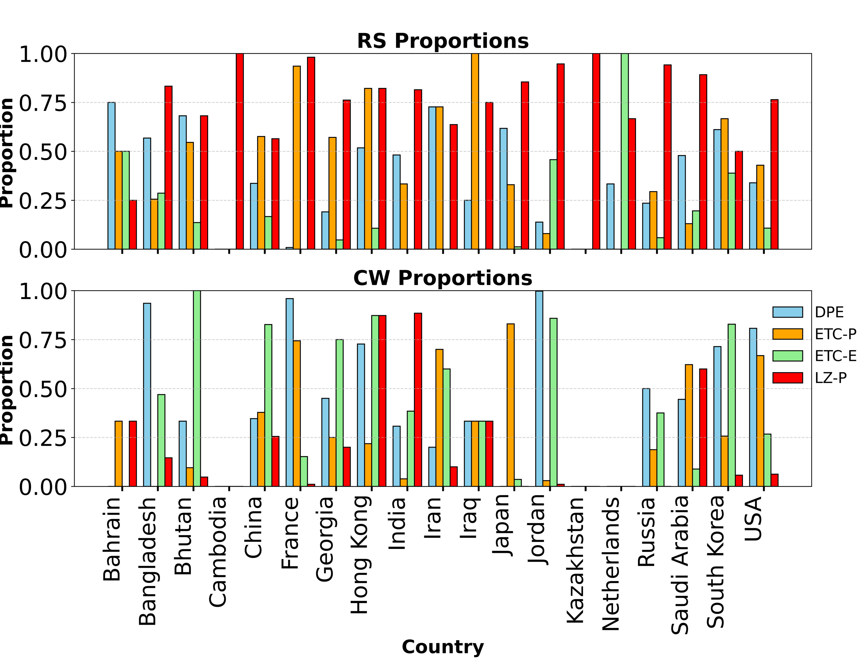
This experiment assesses whether the country-specific initial sequence (CW) or the global Reference Sequence (RS) SARS-CoV-2 (GenBank Accession ID: $NC\_045512.2$) Coronaviridae Study Group of the International Committee on Taxonomy of Viruses [2020] serves as the main cause for the later domestic viral evolution. We test the null hypothesis ($H_{0}$) that the global consensus sequence (RS) causes all subsequent domestic sequences against the alternative ($H_{1}$) that the first sequence reported within a particular country (CW) exerts a stronger influenceSy and Nagaraj [2021] using a dataset of 17,567 high-quality nucleotide sequences from 19 countries in GenBank Database National Center for Biotechnology Information [2026]. Numerical mapping (A=1, C=2, G=3, T=4) is used to evaluate genomic sequences from a variety of countries, such as China, France, and India, across random subsets.

3.5.1 Results: Genomic Causal Analysis of SARS-CoV-2:

We analyzed whether the SARS-CoV-2 consensus sequence (RS) ‘causes’ all other sequences. 16 countries for both $DPE$ and $ETC_{P}$, 11 countries for $ETC_{E}$ and 19 for $LZ_{P}$ out 19 countries had atleast $5\%$ sequences which admitted the $H_{0}$ hypothesis direction. The Figure 8 illustrates that the higher proportions across countries were generally observed under $ETC_{P}$ and $LZ_{P}$ models .

The proportions whether the sequences per country ‘caused’ by CW were greater than RS. $DPE$ shows 10 countries, 14 countries for $ETC_{E}$ and 3 countries for both $ETC_{P}$ and $LZ_{P}$ out of 19 countries. The proportions per country can be seen in the Figure 8.

Figure 8: Genomic causal analysis of SARS-CoV-2: Comparative summary of $DPE$, $ETC_{E}$, $ETC_{P}$, and $LZ_{P}$ sensitivity to global (RS) vs. local (CW) evolutionary drivers.

3.6 Predator-Prey System

$DPE$ was evaluated on a real-world dataset from a prey-predator system Veilleux [1976]Jost and Ellner [2000]. The data consists of 71 data points of predator (Didinium nasutum) and prey (Paramecium aurelia) populations (Figure 9. The predator population influences the prey population directly, and then itself gets influenced by a change in the prey population, indicating a system of bidirectional causation. The direction of causal influence from predator to prey is expected to be higher than in the opposite direction. After removing the initial 9 transients, the remaining 62 data points were considered for this analysis.

Figure 9: Population dynamics of the predator (Didinium nasutum) and prey (Paramecium aurelia).

3.6.1 Results: Predator-Prey System

Table 6: Predator-Prey System: Comparative causal metrics for Predator-Prey interaction across different models.

Model	Direction	Strength	Pred $\rightarrow$ Prey	Prey $\rightarrow$ Pred
$DPE$	Pred $\rightarrow$ Prey	0.1125	0.1700	0.2825
$ETC_{P}$	Pred $\rightarrow$ Prey	1.0000	0.0000	1.0000
$ETC_{E}$	Pred $\rightarrow$ Prey	0.0778	0.8000	0.7222
$LZ_{P}$	Pred $\rightarrow$ Prey	5.0000	2.0000	7.0000

The $DPE$, $ETC_{E}$, and $LZ_{P}$ correctly identify the dominant causal direction from predator to prey. After removal of the first nine transient pairs and analyzing the remaining 62 pairs of samples, the weighted entropy calculated by $DPE$ for the $Predator\rightarrow Prey$ direction is lower than that of the reverse $Prey\rightarrow Predator$ seen in table 6, indicating higher causal certainty in the desired direction ($Predator\rightarrow Prey$). All models, detects the strength of causation from Predator to Prey as higher.

4 Discussion

Table 7 provides a summary of model reliability across experimental settings rather than reporting exact performance values. A framework is considered reliable if it achieves an average accuracy of at least $80\%$ across trials. Thus, the table serves as a binary indicator of consistent performance under each experimental condition. This representation highlights the domains in which each method can be expected to perform robustly, while avoiding overinterpretation of marginal numerical differences.

Table 7: Summary of reliability across experiments. A check mark ($\checkmark$) indicates that the framework achieves an average accuracy of $\geq 80\%$ across trials for the corresponding experiment, while ($\times$) indicates that it does not. The table reflects reliability, not exact performance values.

Experiments	$DPE$	$ETC_{E}$	$ETC_{P}$	$LZ_{P}$
Delayed Bit-flip	$\checkmark$	$\times$	$\times$	$\checkmark$
AR(1) Coupling	$\checkmark$	$\times$	$\times$	$\checkmark$
1D Skew-tent Maps	$\checkmark$	$\times$	$\times$	$\times$
Sparse Processes	$\checkmark$	$\times$	$\times$	$\times$
SARS-CoV-2 (RS vs. CW)	$\times$	$\times$	$\checkmark$	$\checkmark$
Predator-Prey	$\checkmark$	$\checkmark$	$\checkmark$	$\checkmark$

5 Limitations and Future Work

The present study does not explicitly account for the presence of confounding variables. In particular, the proposed framework assumes that the observed asymmetric pattern-level influence arises directly from the candidate cause. A natural extension of this work is to investigate the identification of latent confounders. One possible direction is to detect patterns that act as common triggers in both sequences, suggesting the presence of an unobserved variable influencing $X$ and $Y$ simultaneously.

Another promising direction is to extend the framework toward a counterfactual formulation of causal discovery. Specifically, we aim to investigate whether the removal of a particular trigger pattern from the assumed cause sequence alters the observed transitions in the effect sequence. Such a formulation would allow us to assess causal influence through pattern-level interventions, thereby strengthening the interpretability and robustness of the method.

For the proposed DPE method, in both the unidirectional coupling experiments and the 1D skew tent map experiments, the case corresponding to $\eta=0$ or $\phi=0$ represents true independence between the systems. However, the proposed method as well as all baseline methods considered for comparison fails to correctly identify this regime as independent, instead detecting a spurious directional influence. This limitation indicates that the current decision rule for inferring independence requires further investigation. In particular, the criterion used to distinguish weak causal influence from genuine independence may not be sufficiently stringent in finite-sample settings or in deterministic chaotic systems. To address this issue, future work should incorporate surrogate data analysis and formal statistical significance testing to evaluate the strength and reliability of the inferred causal direction. Establishing appropriate null models and hypothesis-testing procedures would help differentiate true causal structure from artifacts arising due to finite data length, shared dynamics, or intrinsic complexity of the underlying maps.

6 Conclusion

In this work, we introduced a novel Dictionary Based Pattern Entropy ($DPE$) framework for causal discovery from temporal observational data. Beyond inferring causal direction, the proposed approach identifies interpretable sub pattern (algorithmic units) that influence the change in effect variable. This dual capability distinguishes $DPE$ from existing algorithmic information theoretic approaches. Conceptually, the framework operates at the intersection of Algorithmic Information Theory (AIT) and Shannon Information Theory. From the algorithmic standpoint, causation is interpreted as the emergence of compact, rule based patterns in the candidate cause that systematically constrain the effect. A dictionary of recurring patterns is constructed to capture these algorithmic structures. From the information theoretic perspective, entropy based measures quantify the determinism associated with each pattern, thereby linking structured rule extraction with stochastic variability in observational data. The comparative results summarized in Table 7 clarify the relative standing of $DPE$ against competing AIT-based methods ($ETC_{E}$, $ETC_{P}$, and $LZ_{P}$). Using an average accuracy threshold of $80\%$ to determine reliable applicability, $DPE$ demonstrates consistent performance across synthetic dynamical systems (Delayed Bit-flip, AR(1) Coupling, 1D Skew-tent Maps) and structured sparse processes, outperforming or matching competing approaches in most controlled settings. Notably, $DPE$ is the only method that maintains reliability across all synthetic experiments considered. In ecological data, performance across methods is more comparable, whereas in the SARS-CoV-2 mutation analysis, alternative pattern based approaches show competitive advantages over $DPE$. Overall, the results indicate that $DPE$ offers robust and stable causal detection in systems characterized by structured pattern transmission and deterministic influence, while remaining competitive in real-world scenarios. These findings position $DPE$ as a general and interpretable framework for causal discovery, particularly well suited for dynamical systems where causation manifests through identifiable algorithmic sub-patterns rather than purely global complexity measures.

Code Availability

The source code for all experiments, including the implementation of the proposed $DPE$ framework, is publicly available at https://github.com/i-to-the-power-i/dpe-causal-discovery. Conceptualization: Harikrishnan N B; methodology: Harikrishnan N B, Aditi Kathpalia, Shubham, Nithin Nagaraj; software: Shubham Bhilare (Final implementation) Harikrishnan N B (initial prototype); validation: Shubham Bhilare, Harikrishnan N B, Aditi Kathpalia, Nithin Nagaraj; formal analysis: Harikrishnan N B., Shubham Bhilare, Aditi Kathpalia, Nithin Nagaraj; investigation: Shubham Bhilare, Harikrishnan N B, Aditi Kathpalia, Nithin Nagaraj ; writing—original draft preparation: Harikrishnan N B and Shubham Bhilare; writing—review and editing, Harikrishnan N B, Shubham Bhilare, Aditi Kathpalia and Nithin Nagaraj; Funding acquisition: Harikrishnan N B.