Cross-Modal Mapping and Dual-Branch Reconstruction for 2D–3D Multimodal Industrial Anomaly Detection

Abstract

Multimodal industrial anomaly detection benefits from integrating RGB appearance with 3D surface geometry, yet existing unsupervised approaches commonly rely on memory banks, teacher–student architectures, or fragile fusion schemes, limiting robustness under noisy depth, weak texture, or missing modalities. This paper introduces CMDR–IAD, a lightweight and modality-flexible unsupervised framework for reliable anomaly detection in 2D+3D multimodal as well as single-modality (2D-only or 3D-only) settings. CMDR–IAD combines bidirectional 2D$\leftrightarrow$3D cross-modal mapping to model appearance–geometry consistency with dual-branch reconstruction that independently captures normal texture and geometric structure. A two-part fusion strategy integrates these cues: a reliability-gated mapping anomaly highlights spatially consistent texture–geometry discrepancies, while a confidence-weighted reconstruction anomaly adaptively balances appearance and geometric deviations, yielding stable and precise anomaly localization even in depth-sparse or low-texture regions.

On the MVTec 3D-AD benchmark, CMDR–IAD achieves state-of-the-art performance while operating without memory banks, reaching 97.3% image-level AUROC (I-AUROC), 99.6% pixel-level AUROC (P-AUROC), and 97.6% AUPRO. On a real-world polyurethane cutting dataset, the 3D-only variant attains 92.6% I-AUROC and 92.5% P-AUROC, demonstrating strong effectiveness under practical industrial conditions. These results highlight the framework’s robustness, modality flexibility, and the effectiveness of the proposed fusion strategies for industrial visual inspection. Our source code is available at https://github.com/ECGAI-Research/CMDR-IAD/.

[isasi] organization=CNR-ISASI, Institute of Applied Sciences and Intelligent Systems / National Research Council of Italy, addressline=via Monteroni snc, city=Lecce, postcode=73100, country=Italy

[stiima] organization=CNR-STIIMA, Institute of Intelligent Industrial Technologies and Systems for Advanced Manufacturing,addressline=Via G. Amendola 122 D/O, city=Bari, postcode=70126, country=Italy

[IEMN] organization=Institute d’Electronique de Microelectronique et de Nanotechnologie (IEMN) / Universite Polytechnique Hauts de France; Universite de Lille; CNRS, addressline=UMR 8520, city=City, postcode=59313, country=France

1 Introduction

Industrial anomaly detection (IAD) aims to identify defective or atypical products during or after manufacturing, and is therefore a key component of modern quality control pipelines. In practice, collecting representative defective samples is difficult due to their rarity, variability, and the cost of labeling. As a result, most recent methods adopt an unsupervised or one-class setting, where models are trained only on normal (nominal) data and anomalies are detected as deviations from learned regular patterns. While deep learning has significantly advanced anomaly detection in two-dimensional (2D) images, many industrial defects remain challenging to recognize from RGB appearance alone. Variations in illumination, specular reflections, or sensor noise can degrade the reliability of purely image-based approaches, and some defects manifest predominantly as subtle geometric deviations rather than as obvious color or texture changes. To address these challenges, recent research has increasingly turned to multimodal anomaly detection that combines RGB images with three-dimensional (3D) information such as point clouds or depth maps. 3D measurements are largely invariant to lighting and provide explicit shape and surface information, making them highly complementary to RGB signals. The introduction of benchmarks such as MVTec 3D–AD [3] has accelerated this line of work by offering pixel-registered RGB and 3D data, fostering a variety of multimodal anomaly detection methods.

Early multimodal industrial anomaly detection methods, such as BTF and M3DM, extend successful 2D approaches by modeling normality through memory banks of multimodal features, achieving strong performance at the cost of high memory usage and limited inference speed [15, 38]. To improve efficiency, AST adopts a teacher–student architecture, but treats 3D information indirectly, which limits the explicit exploitation of geometric structure [33]. CFM explicitly models cross-modal feature consistency between RGB and 3D data, highlighting the importance of appearance–geometry relationships, yet remains constrained by its multimodal-only assumption [10]. More recent approaches address robustness through cross-modal distillation, joint teacher–student memory mechanisms, and fusion architecture analysis [35, 24, 25], but often introduce architectural complexity or rely on fixed fusion strategies. Existing methods exhibit clear trade-offs between segmentation performance, inference speed, and memory consumption, motivating a lightweight and modality-flexible framework with adaptive fusion.

In this work, we propose a different perspective on multimodal industrial anomaly detection based on explicit cross-modal feature mapping and dual-branch reconstruction. We introduce CMDR–IAD (Cross-Modal Mapping and Dual-Branch Reconstruction for 2D–3D Multimodal Industrial Anomaly Detection), an unsupervised and modality-flexible framework that directly models relationships between RGB-based and 3D-based features while also learning modality-specific reconstructions of normal appearance and geometry. CMDR–IAD employs frozen pretrained encoders for RGB images and point clouds to extract pixel-aligned feature representations, and learns two lightweight mapping networks that project 2D features into the 3D feature space and vice versa. These mappings are trained exclusively on nominal data, capturing cross-modal correspondences characteristic of defect-free samples. In parallel, two independent reconstruction decoders are trained to reproduce normal 2D and 3D features, providing modality-specific cues about deviations from normal patterns.

At inference time, CMDR–IAD combines four complementary signals: 2D reconstruction error, 3D reconstruction error, and two cross-modal mapping discrepancies. An adaptive fusion mechanism converts reconstruction errors into spatial reliability weights and modulates cross-modal discrepancies through a spatially varying gating function. This design allows the model to emphasize the most informative modality at each pixel and suppress noisy responses in regions with unreliable depth or weak visual texture, producing accurate and stable anomaly maps. Importantly, the use of frozen encoders and lightweight mapping and decoding networks results in competitive memory consumption and inference speed, making CMDR–IAD suitable for deployment in real-world industrial inspection systems. Moreover, the 3D reconstruction branch can operate independently in scenarios where only point clouds are available, as demonstrated on a real-world polyurethane cutting dataset.

The contributions presented in this paper can be summarized as follows:

• We propose CMDR–IAD, a modality-flexible cross-modal mapping and dual-branch reconstruction framework for multimodal industrial anomaly detection, which explicitly models 2D–3D feature relationships while preserving modality-specific normal patterns.

• We introduce an adaptive fusion strategy that integrates cross-modal mapping inconsistencies with modality-aware reconstruction deviations through spatial reliability weighting and contrast-based gating, enabling robust anomaly localization under noisy or incomplete 3D measurements.

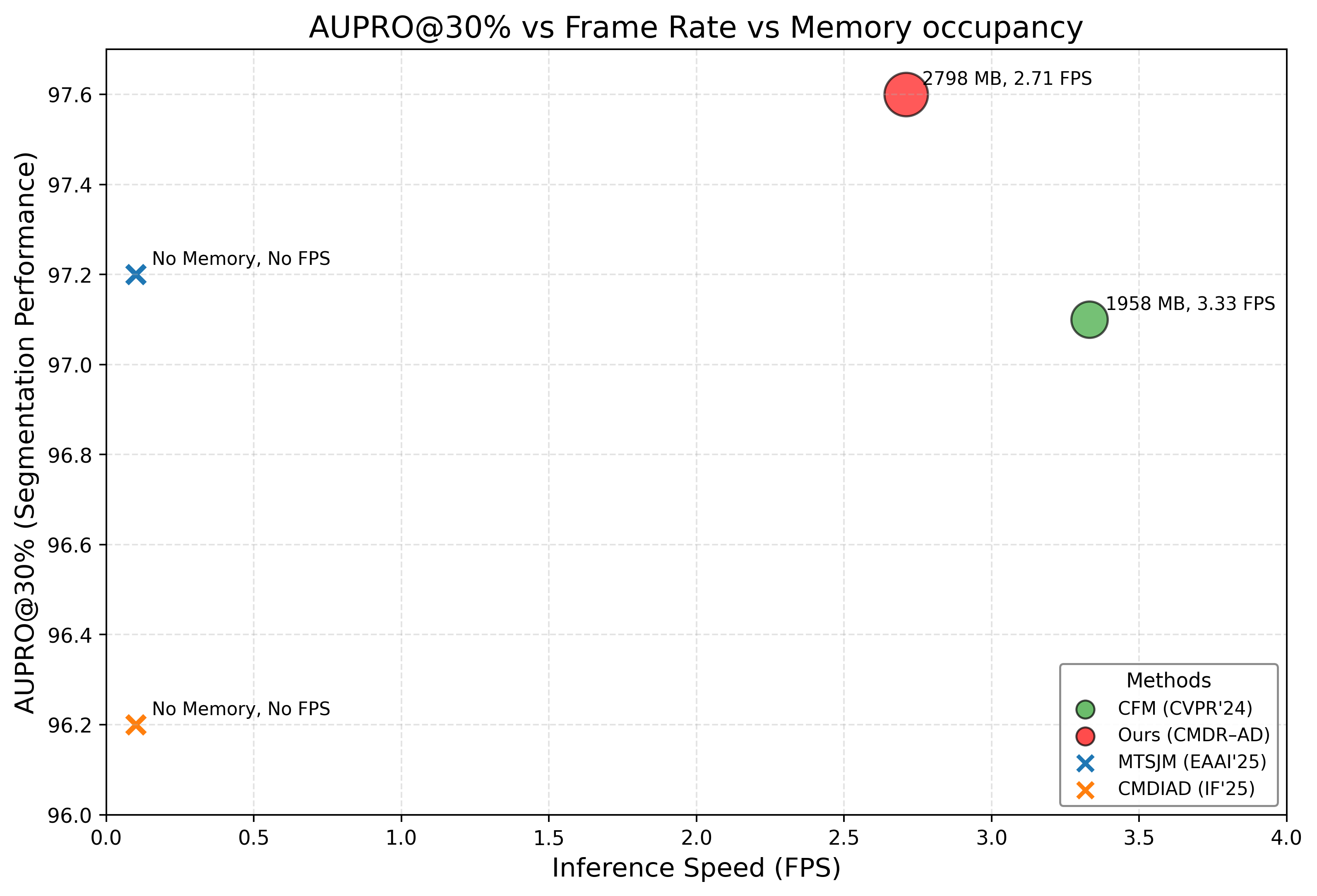
• We demonstrate that CMDR–IAD achieves state-of-the-art anomaly detection and localization performance on the MVTec 3D–AD benchmark while maintaining competitive inference speed and memory footprint (Fig. 1), and we show strong performance of the 3D-only variant on a real polyurethane cutting dataset.

Figure 1: Performance, speed and memory occupancy of Multimodal Anomaly Detection methods. The chart reports defect segmentation performance (AUPRO@30%) vs inference speed.

2 Related Work

2.1 Unsupervised 2D Industrial Anomaly Detection

Unsupervised 2D industrial anomaly detection methods [23] can be broadly grouped into reconstruction-based and feature-embedding-based approaches. Reconstruction-based models rely on autoencoders [37, 1, 4, 16, 31, 42], GANs [6, 40], inpainting networks [29], or diffusion models [39, 36] to reproduce nominal samples and identify anomalies through reconstruction discrepancies. While intuitive, these methods often struggle due to their tendency to partially reconstruct abnormal regions.

Feature-embedding methods instead operate in the latent space [20, 9, 12, 34, 44] of deep networks. Some approaches, such as Deep Feature Reconstruction (DFR) [41], train an autoencoder to reconstruct features extracted from normal samples and detect anomalies via feature-level reconstruction errors. Another popular line of work relies on frozen feature extractors [14, 27, 7, 32, 2], features from normal images are stored in a memory bank during training [45, 19, 32], and test features are compared against this bank to identify deviations. These memory-based approaches achieve strong performance but often suffer from high memory usage and slow inference, as each test feature must be matched against many stored normal features.

2.2 3D-Only Industrial Anomaly Detection

Recent work in 3D-only anomaly detection focuses on identifying geometric defects directly from point clouds without relying on RGB appearance. Teacher–student methods, where a pretrained teacher models local geometric structure and a student learns to regress these features, have demonstrated strong capability in capturing subtle surface deviations [30, 5]. These approaches show that purely geometric information can be highly effective for detecting structural anomalies. This line of research is particularly relevant to the Polyurethane Cutting dataset, where defects arise solely from geometric irregularities. In this setting, our 3D reconstruction pathway achieves strong performance, confirming that accurate modeling of surface geometry alone is sufficient for reliable defect identification and localization.

2.3 Multimodal RGB–3D Industrial Anomaly Detection

The release of the MVTec 3D-AD dataset [3] has significantly accelerated research in industrial anomaly detection involving both RGB appearance and 3D geometry. Initial multimodal baselines explored reconstruction-based strategies—including GANs, VAEs, and autoencoders—to jointly model depth and texture cues. Teacher–student paradigms were later introduced to improve robustness; for example, AST [33] employs asymmetric networks to prevent students from overfitting anomalous patterns in RGB–depth pairs, while DAK-Net [43] introduces dynamic background-guided asymmetric distillation for RGB–3D anomaly detection. Other works enhanced geometric reasoning by integrating handcrafted or learned 3D descriptors, as demonstrated by Horwitz and Hoshen [15].

Memory-bank–driven multimodal approaches extend successful 2D methods to 3D settings. BTF [15] augments frozen 2D CNN features with handcrafted point-cloud descriptors and stores them in a feature bank for nearest-neighbor retrieval. M3DM [38] advances this idea by adopting frozen Transformer-based RGB and 3D backbones trained via large-scale self-supervision, and by introducing a learnable module to fuse 2D and 3D features before inserting them into a large multimodal memory bank. While effective, M3DM suffers from heavy memory usage and slow inference due to expensive feature comparisons.

Inspired by this line of work, CFM [10] replaces memory banks with lightweight cross-modal feature mapping networks that predict one modality from the other and compute anomaly scores directly from feature discrepancies. Further improvements include CMDIAD [35], which employs cross-modal distillation to handle missing or incomplete modalities during inference. MTSJM [24] jointly optimizes multimodal representations through mask-based teacher–student learning and multimodal feature banks, achieving strong performance but still relying on large memory structures. More recently, 3D-ADNAS [25] leverages neural architecture search to identify optimal RGB–3D fusion designs, showing that multimodal AD performance is sensitive to backbone and fusion choices.

In contrast to multimodal fusion strategies in M3DM (2023) [38], CFM (2024) [10], and recent fusion architectures such as MTSJM (2025) [24], CMDIAD (2025) [35], and 3D-ADNAS (2025) [25], DAK-Net (2026) [43], CMDR–IAD introduces explicit 2D$\leftrightarrow$3D cross-modal mapping and dedicated appearance–geometry reconstruction, leading to state-of-the-art results on MVTec 3D-AD.

3 Methodology

Our proposed unsupervised CMDR–IAD (Cross-Modal Mapping and Dual-Branch Reconstruction for 2D–3D Multimodal Industrial Anomaly Detection) integrates complementary RGB images $I^{2D}$, and point clouds $P^{3D}$ to detect both appearance- and geometry-related anomalies. CMDR–IAD aligns 2D and 3D feature spaces via cross-modal mapping networks while learning modality-specific reconstruction branches that capture normal patterns unique to each modality.

As illustrated in Fig. 2, the framework consists of four core components:

1. Multimodal Feature Extractors – frozen pretrained 2D and 3D encoders producing appearance features $F^{2D}$ and geometric features $F^{3D}$.

2. Cross-Modal Mapping Networks – lightweight MLPs projecting features between modalities to enforce 2D $\leftrightarrow$ 3D consistency.

3. Dual-Branch Reconstruction Modules – independent 2D and 3D decoders reconstructing modality-specific features to model normal appearance and geometry patterns.

4. Reliability-Aware Multimodal Fusion – a reliability- and confidence-aware fusion of cross-modal mapping discrepancies and reconstruction errors for robust anomaly localization.

Modality-flexible operation. CMDR–IAD supports both multimodal and single-modality operation, enabling reliable anomaly detection with complete or missing sensory inputs. Specifically, we consider two operational scenarios:

• Multimodal setting (MVTec 3D-AD): the full 2D+3D pipeline is employed, leveraging bidirectional cross-modal mapping together with both reconstruction branches to model appearance–geometry consistency.

• 3D-only setting (Polyurethane dataset): only the 3D pathway (Point-MAE encoder + Decoder3D) is used, supported by a dedicated point-cloud preprocessing pipeline.

Figure 2: Overview of the proposed CMDR–IAD framework. The method integrates RGB images and point clouds through multimodal feature extraction, cross-modal mapping, and dual-branch 2D–3D reconstruction. Cross-modal discrepancy maps and reconstruction errors are fused into the final anomaly map $\Psi$, enabling robust detection of both appearance- and geometry-related defects.

3.1 Multimodal Feature Extractors

Appearance and geometric features are extracted from the RGB image $I^{2D}$ and point cloud $P^{3D}$ using pretrained encoders that remain frozen throughout training.

2D Feature Extraction. Given an RGB image $I^{2D}$, the 2D encoder ${E}_{2D}$ (DINO ViT-B) produces a low-resolution feature map $F^{2D}_{raw}$. Since its spatial resolution is smaller than that of the original image, we apply bilinear upsampling to obtain a dense pixel-aligned representation

$$F^{2D}\in\mathbb{R}^{H\times W\times D_{2D}},$$

providing one appearance feature vector per pixel.

3D Feature Extraction. The point cloud $P^{3D}$ is processed by the 3D encoder ${E}_{3D}$ (Point-MAE/PointTransformer), producing a set of geometric feature tokens $F^{3D}_{raw}$ associated with only a subset of points. Since many 3D feature extractors do not compute features for every input point but only for selected point groups [28], we interpolate features for all remaining points by using their nearest feature centers. Following a strategy similar to [38], each point feature is computed from the features of its closest centers. This yields a dense per-point geometric representation

$$F^{3D}_{pts}\in\mathbb{R}^{N\times D_{3D}}.$$

Feature Alignment. The pixel–point correspondences in MVTec 3D-AD [3] enable the integration of point-wise features into the image grid, yielding a dense representation of geometric information.

$$F^{3D}\in\mathbb{R}^{H\times W\times D_{3D}}.$$

Pixels without a corresponding 3D point are initialized to zero. To improve spatial coherence and suppress isolated artifacts introduced by sparse projections, we apply a light spatial smoothing implemented as a channel-wise 2D average pooling with a $3\times 3$ kernel and stride $1$. Since no padding is used, the smoothed feature map is subsequently resized to the target resolution using adaptive average pooling.

At the end of this stage, the multimodal feature extractors produce two pixel-aligned feature maps:

$$F^{2D}={E}_{2D}(I^{2D}),\qquad F^{3D}={E}_{3D}(P^{3D}),$$

which serve as the input to the cross-modal mapping networks and the dual-branch reconstruction modules.

3.2 Cross-Modal Mapping Networks

The cross-modal mapping stage explicitly models the correspondence between appearance features $F^{2D}$ and geometric features $F^{3D}$. CMDR–IAD employs two lightweight multilayer perceptrons (MLPs), $\mathcal{M}_{2D\rightarrow 3D}$ and $\mathcal{M}_{3D\rightarrow 2D}$, each composed of an input projection, a nonlinear transformation block (GELU + LayerNorm), and an output projection. For each pixel location $i$ with aligned multimodal features, the mappings predict the corresponding feature in the other modality as

$$\hat{F}^{3D}_{map}(i)=\mathcal{M}_{2D\rightarrow 3D}\big(F^{2D}(i)\big),\qquad\hat{F}^{2D}_{map}(i)=\mathcal{M}_{3D\rightarrow 2D}\big(F^{3D}(i)\big).$$

If no valid 3D feature is available at location $i$ (e.g., due to missing depth or occlusion), the mapped feature is set to zero to avoid introducing invalid supervision. Setting mapped features to zero at locations with missing 3D observations prevents spurious cross-modal supervision from unreliable geometry, improving training stability. This masking avoids enforcing artificial appearance–geometry consistency in depth-sparse regions, thereby preserving anomaly sensitivity while allowing modality-specific reconstruction cues to dominate.

After processing all pixel locations, the mapping networks yield dense cross-modal prediction maps:

$$\hat{F}^{3D}_{map}=\mathcal{M}_{2D\rightarrow 3D}(F^{2D}),\qquad\hat{F}^{2D}_{map}=\mathcal{M}_{3D\rightarrow 2D}(F^{3D}).$$

3.3 Dual-Branch Reconstruction Modules

To capture modality-specific normal patterns, CMDR–IAD employs two independent reconstruction branches: a 2D decoder $\mathcal{D}_{2D}$ and a 3D decoder $\mathcal{D}_{3D}$. Each branch operates solely within its own modality, enabling precise modeling of appearance cues in RGB images and geometric structures in point clouds.

2D Reconstruction Branch (Fig. 3). Given the 2D feature map $F^{2D}$, $\mathcal{D}_{2D}$ first projects the features to a compact latent space using linear layers with GELU and LayerNorm. A sparse-attention block is then applied to enhance local contextual dependencies, followed by an MLP refinement with residual connections. The refined features are reshaped into a spatial grid and decoded through ConvTranspose2D layers to produce the reconstructed feature map

$$\hat{F}^{2D}_{rec}=\mathcal{D}_{2D}(F^{2D}).$$

Figure 3: Overview of the 2D Reconstruction Branch. Projected features are enhanced using a sparse-attention block and an MLP refinement module with residual connections, then decoded through ConvTranspose2D layers to generate the reconstructed 2D feature map.

3D Reconstruction Branch (Fig. 4). The 3D decoder $\mathcal{D}_{3D}$ processes the geometric feature map $F^{3D}$ through a projection layer and a sequence of ConvTranspose1D layers to restore the original resolution. A lightweight channel-attention module is applied to emphasize informative geometric features, yielding the reconstructed representation

$$\hat{F}^{3D}_{rec}=\mathcal{D}_{3D}(F^{3D}).$$

Figure 4: Overview of the 3D Reconstruction Branch. After projection and ConvTranspose1D upsampling, a gating block refines the features through sequential 1D convolutions and a sigmoid mask, which is multiplied with a residual pathway to produce the final 3D reconstruction.

3.4 Training Objective

CMDR–IAD optimizes the cross-modal mapping networks and reconstruction decoders independently, without a joint loss. Each module is trained using a masked cosine similarity loss computed only at locations with valid 2D–3D correspondences.

Masked Similarity Loss. We build upon the cosine similarity formulation commonly used in prior feature-alignment work [10] and adapt it to a masked setting.

Given a predicted feature $\hat{F}$ and its target feature $F$, we define

$$\mathcal{L}_{sim}(F,\hat{F})=1-\cos(F,\hat{F}),$$

which is evaluated only over pixels with valid 3D features using a binary mask.

Mapping and Reconstruction Losses. The two mapping networks are trained as

$$\mathcal{L}_{map}^{2D}=\mathcal{L}_{sim}\!\left(F^{2D},\hat{F}^{2D}_{map}\right),\qquad\mathcal{L}_{map}^{3D}=\mathcal{L}_{sim}\!\left(F^{3D},\hat{F}^{3D}_{map}\right),$$

while the reconstruction decoders are optimized via

$$\mathcal{L}_{rec}^{2D}=\mathcal{L}_{sim}\!\left(F^{2D},\hat{F}^{2D}_{rec}\right),\qquad\mathcal{L}_{rec}^{3D}=\mathcal{L}_{sim}\!\left(F^{3D},\hat{F}^{3D}_{rec}\right).$$

Each loss updates only its corresponding module, allowing all branches to be trained independently. This design avoids cross-modal gradient interference and promotes stable and specialized learning

3.5 Anomaly Scoring and Reliability-Aware Multimodal Fusion

At inference time, CMDR–IAD computes anomaly scores by jointly analyzing cross-modal mapping discrepancies and modality-specific reconstruction errors. Feature discrepancies are measured using a normalized Euclidean distance. Given two feature vectors $a$ and $b$, we define

$$d(a,b)=\left\lVert\frac{a}{\lVert a\rVert_{2}}-\frac{b}{\lVert b\rVert_{2}}\right\rVert_{2},$$

which corresponds to the $\ell_{2}$ distance between $\ell_{2}$-normalized features.

Reliability-Gated Mapping Anomaly. Cross-modal mapping discrepancies are computed independently for each modality as

$$d^{2D}_{map}(x,y)=d\!\left(\hat{F}^{2D}_{map}(x,y),F^{2D}(x,y)\right),\qquad d^{3D}_{map}(x,y)=d\!\left(\hat{F}^{3D}_{map}(x,y),F^{3D}(x,y)\right).$$

To emphasize spatially consistent appearance–geometry inconsistencies, the two discrepancies are combined into a joint mapping anomaly

$$d_{\text{joint}}(x,y)=d^{2D}_{map}(x,y)\cdot d^{3D}_{map}(x,y).$$

A spatial reliability gate $\alpha(x,y)\in[0,1]$ is derived from local statistics of $d_{\text{joint}}$ and reflects the confidence of cross-modal agreement. The resulting reliability-gated mapping anomaly is defined as

$$A_{\text{map}}(x,y)=\alpha(x,y)\,d_{\text{joint}}(x,y).$$

Confidence-Weighted Reconstruction Anomaly. Reconstruction discrepancies are computed independently for each modality:

$$d^{2D}_{rec}(x,y)=d\!\left(\hat{F}^{2D}_{rec}(x,y),F^{2D}(x,y)\right),\qquad d^{3D}_{rec}(x,y)=d\!\left(\hat{F}^{3D}_{rec}(x,y),F^{3D}(x,y)\right).$$

Each modality is assigned a confidence weight inversely related to its reconstruction error:

$$w_{2}(x,y)=\exp\!\left(-B\,d^{2D}_{rec}(x,y)\right),\qquad w_{3}(x,y)=\exp\!\left(-B\,d^{3D}_{rec}(x,y)\right),$$

where $B$ is a temperature parameter controlling the sharpness of the weighting, set to $B=0.3$ in all experiments.

The confidence-weighted reconstruction anomaly is then defined as

$$A_{\text{rec}}(x,y)=\frac{w_{2}(x,y)\,d^{2D}_{rec}(x,y)+w_{3}(x,y)\,d^{3D}_{rec}(x,y)}{w_{2}(x,y)+w_{3}(x,y)+\varepsilon}.$$

Final Anomaly Map. The final pixel-level anomaly score integrates cross-modal reliability and modality-specific confidence as

$$\Psi_{\text{full}}(x,y)=A_{\text{map}}(x,y)\cdot A_{\text{rec}}(x,y),$$

followed by light spatial smoothing using box filters to improve localization stability.

Image-Level Anomaly Scoring. The smoothed anomaly map $\Psi$ is normalized over valid pixels. For image-level anomaly detection, we compute a scalar score

$$S=\max_{x,y}\frac{\Psi(x,y)}{\sqrt{\overline{\Psi}_{valid}+\varepsilon}},$$

where $\overline{\Psi}_{valid}$ denotes the mean of $\Psi$ over unmasked pixels. The score $S$ is used for image-level anomaly detection, while $\Psi$ provides fine-grained pixel-level anomaly localization.

3.6 3D-Only Inference Mode for Polyurethane Cuts

The polyurethane cutting dataset provides only 3D point clouds without registered RGB images. Accordingly, CMDR–IAD operates in a dedicated 3D-only inference mode, where only the geometric branch of the framework is activated. In this setting, raw point clouds are first processed using the preprocessing pipeline described in in Sec. 4 and then passed to the frozen 3D encoder ${E}_{3D}$ and the 3D decoder $\mathcal{D}_{3D}$ to identify structural irregularities on cutting surfaces.

Feature Extraction. Each point cloud $P^{3D}$ is processed by ${E}_{3D}$ to produce a dense geometric feature representation:

$$F^{3D}={E}_{3D}(P^{3D}).$$

Since no RGB modality is available, cross-modal mapping and 2D reconstruction are disabled.

3D Reconstruction and Anomaly Scoring. The decoder $\mathcal{D}_{3D}$ reconstructs the expected normal geometry:

$$\hat{F}^{3D}_{rec}=\mathcal{D}_{3D}(F^{3D}).$$

Per-point anomaly scores are computed as the normalized Euclidean distance

$$A^{3D}_{rec}(i)=\left\|\tilde{F}^{3D}(i)-\tilde{\hat{F}}^{3D}_{rec}(i)\right\|_{2},$$

where $\ell_{2}$-normalization is applied to both feature vectors. The resulting anomaly map is smoothed using the same box-filter strategy adopted in the multimodal setting.

Image-Level Decision. An image-level anomaly score is obtained by max pooling:

$$S=\max_{i}A^{3D}_{rec}(i),$$

which is used for image-level AUROC evaluation, while $A^{3D}_{rec}$ supports pixel-level AUROC computation.

Despite the absence of RGB cues, the 3D-only variant of CMDR–IAD remains effective for polyurethane cuts, as defects such as irregular cuts, burrs, gaps, and shape distortions are strongly expressed in the geometric modality. The robust feature representation of ${E}_{3D}$ enables reliable anomaly detection in this unimodal setting.

4 Datasets and Preprocessing

To evaluate CMDR–IAD under both multimodal and single-modality conditions, we use two datasets: MVTec 3D–AD for RGB+3D evaluation and a real-world polyurethane cutting dataset to validate the 3D-only branch of the model.

4.1 MVTec 3D–AD Setup

MVTec 3D–AD contains 10 industrial object categories with 2656 training samples and 1197 test samples [3]. Following the standard anomaly detection protocol, only normal samples are used for training, while the test set includes both normal and defective instances. Each sample provides an RGB image and a pixel-registered 3D representation storing $(x,y,z)$ coordinates.

MVTec 3D–AD serves as the primary multimodal benchmark for CMDR–IAD. In this setting, the full 2D+3D pipeline is employed during inference, including both feature extractors, cross-modal mapping networks, and reconstruction branches, enabling evaluation of appearance–geometry consistency.

4.2 Polyurethane 3D Dataset and Preprocessing Pipeline

The polyurethane cutting dataset was collected within the MOROSAI project using a dual-sensor profilometer with a 405 nm laser. The scanning system outputs dense 3D point clouds focused on the cutting edges of large polyurethane samples. Since only geometric data is available, this dataset is used to evaluate the 3D-only inference mode of CMDR–IAD.

The raw point clouds are processed by a three-stage preprocessing pipeline.

Extraction of Geometric Outliers Using Isolation Forest

Given a point cloud

$$P=\{p_{i}\in\mathbb{R}^{3}\}_{i=1}^{N},$$

we apply an unsupervised Isolation Forest (ISO) [22] to detect sparse geometric outliers caused by cutting defects or sensor noise. ISO is a tree-based unsupervised anomaly detection method and is well suited for large-scale, high-dimensional point cloud data. A low-contamination setting ($\gamma=0.0001$) is adopted due to the sparsity of polyurethane defects, as higher contamination levels may lead to false positives. ISO outputs a binary point-level abnormality mask for each scan, used in subsequent processing.

Sequential Chunking and Chunk-Level Labeling

Each point cloud is sequentially partitioned into fixed-size chunks of 9216 points, following common practice for large-scale point cloud processing [13].

Let $C_{k}$ denote the $k$-th chunk and $m_{i}$ the ISO-based binary outlier indicator for point $p_{i}$. The abnormal ratio of each chunk is

$$f_{k}=\frac{1}{|C_{k}|}\sum_{p_{i}\in C_{k}}m_{i}.$$

A chunk is labeled anomalous if $f_{k}\geq\tau$, with $\tau=0.0025$. For each scan, we store the chunked point clouds, their chunk-level labels, and the corresponding per-point abnormal masks.

Global Dataset Construction and Normalization

All chunks are aggregated into global data, label, and point-level mask files. Following a one-class anomaly detection protocol, only normal chunks are used for training, with a 90/10 split applied to the normal subset. This results in 1856 normal samples for training and a test set of 235 samples, comprising 207 normal and 28 anomalous instances.

Each chunk is independently normalized using min–max scaling to the range $[-1,1]$ [18]. The resulting train and test splits, together with their corresponding point-level masks are used to train and evaluate the 3D reconstruction branch of CMDR–IAD.

5 Experiments

5.1 Datasets and Evaluation Metrics

We evaluate CMDR–IAD on the MVTec 3D–AD benchmark [3] and a real polyurethane cutting dataset (Section 4). MVTec 3D–AD provides pixel-aligned RGB and 3D data for multimodal evaluation, while the polyurethane dataset consists of sequential 3D point-cloud blocks and is used to assess the 3D-only inference mode.

Performance is evaluated following the MVTec 3D–AD protocol. Image-level anomaly detection performance is measured using the Area Under the Receiver Operating Characteristic Curve (I-AUROC). Pixel-level anomaly localization is primarily evaluated using the Area Under the Per-Region Overlap (AUPRO). The experimental evaluation in the main paper is conducted using I-AUROC%, AUPRO@30% and AUPRO@1%. Pixel-level AUROC (P-AUROC) results are provided in the Appendix (Table 9) for completeness.

For the polyurethane dataset, I-AUROC corresponds to block-level anomaly classification, while point-level localization is evaluated using P-AUROC against ISO-based ground-truth masks. This dual evaluation protocol enables assessment of both coarse and fine-grained anomaly behavior in the 3D-only setting.

5.2 Implementation Details

Following M3DM [38] and CFM [10], we employ frozen pretrained Transformers as feature extractors: DINO ViT-B/8 [7] trained on ImageNet [11] for RGB images, and Point-MAE [28] trained on ShapeNet [8] for point clouds. For MVTec 3D–AD, both RGB images and pixel-aligned 3D features are aligned on a $224\times 224$ spatial grid .

Only the cross-modal mapping networks and the reconstruction decoders are trained. For each MVTec 3D–AD category, the four modules $\mathcal{M}_{2D\rightarrow 3D}$, $\mathcal{M}_{3D\rightarrow 2D}$, $\mathcal{D}_{2D}$, and $\mathcal{D}_{3D}$ are optimized independently using the masked cosine similarity loss described in Sec 3. Training is performed with the Adam optimizer [17], learning rate $10^{-3}$, batch size 1, and 50 epochs.

For the polyurethane cutting dataset, CMDR–IAD operates in a 3D-only setting. Only the 3D reconstruction decoder is trained using Point-MAE features. Each sample is represented as a $96\times 96$ pseudo-image corresponding to 9216 points, and training is performed with AdamW [26], learning rate $10^{-3}$, batch size 4, for 50 epochs.

Experimental results are obtained on a workstation configured with an NVIDIA A100 GPU (40960 MiB).

Inference Speed and Memory Evaluation. Inference speed is measured in frames per second (FPS) on the same hardware for all datasets, including MVTec 3D–AD and the polyurethane cutting dataset. We report the average inference time over all test samples, including input pre-processing and all subsequent steps up to anomaly score computation. All GPU operations are synchronized before timing. Memory footprint is measured during inference and accounts for network parameters, intermediate activations, and auxiliary buffers.

5.3 Results on MVTec 3D-AD dataset

5.3.1 Quantitative Results.

Table 1 reports the image-level I-AUROC results on the MVTec 3D-AD dataset. We compare our method with recent single-modality and multimodal approaches, including AST [33], M3DM [38], CFM [10], CMDIAD [35], MTSJM [24], 3D-ADNAS [25], and DAK-Net [43].

2D results. In the 2D setting, CMDR–IAD achieves the highest I-AUROC on Peach, Potato, and Tire, being the only method exceeding 90% on both Potato and Tire. It outperforms the second-best methods by more than 16% on Potato and 11.7% on Tire, while attaining the second-highest performance on Rope. The mean I-AUROC of 87.5% remains competitive with strong baselines such as AST, M3DM, MTSJM, and CMDIAD, despite 3D-ADNAS achieving the highest overall 2D mean.

3D results. In the 3D setting, CMDR–IAD achieves the highest I-AUROC on Cable Gland, Foam, Rope, and Tire, while attaining the second-highest performance on Peach. Notably, it is the only method exceeding 90% on Foam and Tire, outperforming the second-best results by 14.6% and 8.3%, respectively. CMDR–IAD also achieves the second-highest mean I-AUROC (87.5%), demonstrating strong and consistent performance across categories.

2D+3D multimodal results. In the multimodal setting, CMDR–IAD achieves the highest I-AUROC on 5 out of 10 object categories. Notably, CMDR–IAD is the only method whose I-AUROC consistently exceeds 93% across all classes, with scores ranging from 93.0% to 99.8%. This leads to a mean I-AUROC of 97.3%, surpassing strong multimodal baselines such as AST, M3DM, CFM, MTSJM, CMDIAD, 3D-ADNAS, and DAK-Net by up to 1.6%, thereby establishing a new state of the art on MVTec 3D–AD. These results highlight the effectiveness of our reliability-aware fusion, which jointly leverages reconstruction confidence and cross-modal consistency to achieve robust and well-balanced anomaly detection across diverse object categories.

Table 1: I-AUROC (%) for anomaly detection on all classes of the MVTec 3D-AD dataset. The best results are highlighted in bold, while the second-best are underlined. Our approach delivers competitive performance in single-modality (2D and 3D) settings and achieves state-of-the-art results in the multimodal (2D+3D) configuration.

Method	Bagel	Cable Gland	Carrot	Cookie	Dowel	Foam	Peach	Potato	Rope	Tire	Mean
2D
PatchCore (2022) [32]	87.6	88.0	79.1	68.2	91.2	70.1	69.5	61.8	84.1	70.2	77.0
BTF (2023)[15]	87.6	88.0	79.1	68.2	91.2	70.1	69.5	61.8	84.1	70.2	77.0
BTM (2024) [21]	90.9	89.5	83.8	74.5	97.5	71.4	79.0	60.5	93.0	75.9	81.6
AST (2023) [33]	94.7	92.8	85.1	82.5	98.1	95.1	89.5	61.3	99.2	82.1	88.0
M3DM (2023) [38]	94.4	91.8	89.6	74.9	95.9	76.7	91.9	64.8	93.8	76.7	85.0
MTSJM (2025) [24]	97.1	90.8	94.2	73.1	96.7	79.5	98.4	60.8	83.8	83.3	85.8
CMDIAD (2025) [35]	94.2	91.8	89.6	74.9	95.9	76.7	91.9	64.8	94.1	76.8	85.1
3D-ADNAS (2025) [25]	98.1	98.8	92.7	95.6	94.2	92.8	85.3	79.1	97.7	85.8	92.0
CMDR–IAD (Ours)	82.4	63.6	77.8	81.0	95.4	84.3	99.0	95.2	98.4	97.5	87.5
3D
Depth GAN (2022) [3]	53.0	37.6	60.7	60.3	49.7	48.4	59.5	48.9	53.6	52.1	52.4
Depth AE (2022) [3]	46.8	73.1	49.7	67.3	53.4	41.7	48.5	54.9	56.4	54.6	54.6
Depth VM (2022) [3]	51.0	54.2	46.9	57.6	60.9	69.9	45.0	41.9	66.8	52.0	54.6
Voxel GAN (2022) [3]	38.3	62.3	47.4	63.9	56.4	40.9	61.7	42.7	66.3	57.7	53.8
Voxel AE (2022) [3]	69.3	42.5	51.5	79.0	49.4	55.8	53.7	48.4	63.9	58.3	57.2
Voxel VM (2022) [3]	75.0	74.7	61.3	73.8	82.3	69.3	67.9	65.2	60.9	69.0	69.9
3D-ST (2023) [5]	86.2	48.4	83.2	89.4	84.8	66.3	76.3	68.7	95.8	48.6	74.8
BTF (2023) [15]	82.5	55.1	95.2	79.7	88.3	58.2	75.8	88.9	92.9	65.3	78.2
BTM (2024)[21]	93.9	55.3	91.6	84.4	82.3	58.8	71.8	92.8	97.6	63.3	79.2
AST (2023) [33]	88.1	57.6	96.5	95.7	67.9	79.7	99.0	91.5	95.6	61.1	83.3
M3DM (2023) [38]	94.1	65.1	96.5	96.9	90.5	76.0	88.0	97.4	92.6	76.5	87.4
MTSJM (2025) [24]	98.5	72.8	96.1	99.1	87.6	77.3	90.6	93.5	93.2	85.6	89.4
CMDIAD (2025) [35]	97.3	68.7	92.7	96.5	83.8	73.2	85.7	98.7	86.4	86.3	86.0
3D-ADNAS (2025) [25]	79.4	85.7	69.9	94.6	69.5	68.6	70.5	87.3	95.3	66.7	78.8
CMDR–IAD (Ours)	68.4	89.9	81.9	84.2	86.5	94.3	93.4	84.3	98.1	94.4	87.5
2D+3D
Depth GAN (2022) [3]	53.8	37.2	58.0	60.3	43.0	53.4	64.2	60.1	44.3	57.7	53.2
Depth AE (2022) [3]	64.8	50.2	65.0	48.8	80.5	52.2	71.2	52.9	54.0	55.2	59.5
Depth VM (2022) [3]	51.3	55.1	47.7	58.1	61.7	71.6	45.0	42.1	59.8	62.3	55.5
Voxel GAN (2022) [3]	68.0	32.4	56.5	39.9	49.7	48.2	56.6	57.9	60.1	48.2	51.7
Voxel AE (2022) [3]	51.0	54.0	38.4	69.3	44.6	63.2	55.0	49.4	72.1	41.3	53.8
Voxel VM (2022) [3]	55.3	77.2	48.4	70.1	75.1	57.8	48.0	46.6	68.9	61.1	60.9
3D-ST (2023) [5]	95.0	48.3	98.6	92.1	90.5	63.2	94.5	98.8	97.6	54.2	83.3
BTM (2024) [21]	98.0	86.0	98.0	96.3	97.8	72.6	95.8	95.3	98.0	92.6	93.0
BTF (2023) [15]	91.8	74.8	96.7	88.3	93.2	58.2	89.6	91.2	92.1	88.6	86.5
AST (2023) [33]	98.3	87.3	97.6	97.1	93.2	88.5	97.4	98.1	100.0	79.7	93.7
M3DM (2023) [38]	99.4	90.9	97.2	97.6	96.0	94.2	97.3	89.9	97.2	85.0	94.5
CFM (2024) [10]	99.4	88.8	98.4	99.3	98.0	88.8	94.1	94.3	98.0	95.3	95.4
MTSJM (2025) [24]	100.0	93.1	98.5	99.4	96.8	89.9	98.6	94.7	96.2	89.7	95.7
CMDIAD (2025) [35]	99.2	89.3	97.7	96.0	95.3	88.3	95.0	93.7	94.3	89.3	93.8
3D-ADNAS (2025) [25]	99.7	100.0	97.1	98.6	96.6	94.8	89.7	87.3	100.0	86.7	95.1
DAK-Net (2026) [43]	96.8	90.0	97.3	97.2	98.6	93.9	95.2	87.6	99.4	80.0	93.6
CMDR–IAD (Ours)	99.6	93.0	98.6	99.8	99.1	93.6	99.6	93.1	98.7	97.5	97.3

Table 2: AUPRO@30% for anomaly detection on all classes of the MVTec 3D-AD dataset. The best results are highlighted in bold, while the second-best are underlined. Our approach delivers competitive performance in single-modality (2D and 3D) settings and achieves state-of-the-art localization accuracy in the multimodal (2D+3D) configuration.

Method	Bagel	Cable Gland	Carrot	Cookie	Dowel	Foam	Peach	Potato	Rope	Tire	Mean
2D
PatchCore (2022) [32]	90.1	94.9	92.8	87.7	89.2	56.3	90.4	93.2	90.8	90.6	87.6
BTF (2023) [15]	90.1	94.9	92.8	87.7	89.2	56.3	90.4	93.2	90.8	90.6	87.6
BTM (2024) [21]	90.1	95.8	94.2	90.5	95.1	61.5	90.6	93.8	92.7	91.6	89.6
AST (2023) [33]	83.4	87.4	76.4	44.7	87.2	56.9	84.5	51.8	86.3	58.8	71.7
M3DM (2023) [38]	95.2	97.2	97.3	89.1	93.2	84.3	97.0	95.6	96.8	96.6	94.2
MTSJM (2025) [24]	97.6	96.9	97.5	91.4	94.9	86.9	97.5	96.3	97.0	96.6	95.3
CMDIAD (2025) [35]	95.1	97.2	97.3	89.1	93.2	84.3	97.0	95.6	96.8	96.6	94.2
CMDR–IAD (Ours)	95.2	96.3	83.1	96.9	97.5	85.1	90.7	98.1	96.3	96.0	93.5
3D
Depth GAN (2022) [3]	11.1	7.2	21.2	17.4	16.0	12.8	0.3	4.2	44.6	7.5	14.3
Depth AE (2022) [3]	14.7	6.9	29.3	21.7	20.7	18.1	16.4	6.6	54.5	14.2	20.3
Depth VM (2022) [3]	28.0	37.4	24.3	52.6	48.5	31.4	19.9	38.8	54.3	38.5	37.4
Voxel GAN (2022) [3]	44.0	45.3	87.5	75.5	78.2	37.8	39.2	63.9	77.5	38.9	58.3
Voxel AE (2022) [3]	26.0	34.1	58.1	35.1	50.2	23.4	35.1	65.8	1.5	18.5	34.8
Voxel VM (2022) [3]	45.3	34.3	52.1	69.7	68.0	28.4	34.9	63.4	61.6	34.6	49.2
BTF (2023) [15]	97.3	87.9	98.2	90.6	89.2	73.5	97.7	98.2	95.6	96.1	92.4
BTM (2024) [21]	97.4	86.1	98.1	93.7	95.9	66.1	97.8	98.3	98.0	94.7	92.6
AST (2023) [33]	95.4	72.3	97.4	90.1	83.2	82.6	97.6	98.2	89.2	75.1	88.1
M3DM (2023) [38]	94.3	81.8	97.7	88.2	88.1	74.3	95.8	97.4	95.0	92.9	90.6
MTSJM (2025) [24]	92.9	85.5	97.1	88.7	87.8	76.4	94.0	97.1	93.7	95.1	90.8
CMDIAD (2025) [35]	94.7	82.6	97.7	88.2	88.1	76.7	96.7	97.8	94.7	94.0	91.1
CMDR–IAD (Ours)	81.2	97.9	76.3	96.6	97.9	92.8	90.8	97.4	97.0	96.8	92.5
2D+3D
Depth GAN (2022) [3]	42.1	42.2	77.8	69.6	49.4	25.2	28.5	36.2	40.2	63.1	47.4
Depth AE ( 2022) [3]	43.2	15.8	80.8	49.1	84.1	40.6	26.2	21.6	71.6	47.8	48.1
Depth VM (2022) [3]	38.8	32.1	19.4	57.0	40.8	28.2	24.4	34.9	26.8	33.1	33.5
Voxel GAN (2022) [3]	66.4	62.0	76.6	74.0	78.3	33.2	58.2	79.0	63.3	48.3	63.9
Voxel AE (2022) [3]	46.7	75.0	80.8	55.0	76.5	47.3	72.1	91.8	1.9	17.0	56.4
Voxel VM (2022) [3]	51.0	33.1	41.3	71.5	68.0	27.9	30.0	50.7	61.1	36.6	47.1
3D-ST ( 2023)[5]	95.0	48.3	98.6	92.1	90.5	63.2	94.5	98.8	97.6	54.2	83.3
BTF (2023) [15]	97.6	96.9	97.9	97.3	93.3	88.8	97.5	98.1	95.0	97.1	95.9
BTM (2024) [21]	97.9	97.2	98.0	97.6	97.7	90.5	97.8	98.2	96.8	97.5	96.9
BTF (2023) [15]	97.6	96.9	97.9	97.3	93.3	88.8	97.5	98.1	95.0	97.1	95.9
AST (2023) [33]	97.0	94.7	98.1	93.6	91.2	91.8	97.9	98.3	88.7	94.2	94.6
M3DM (2023) [38]	97.0	97.1	97.9	95.0	94.1	93.2	97.7	97.1	97.1	97.5	96.4
CFM(2024) [10]	97.9	97.2	98.2	94.5	95.0	96.8	98.0	98.2	97.5	98.1	97.1
MTSJM (2025) [24]	98.4	98.1	98.3	96.8	93.9	95.1	97.7	98.5	97.4	97.3	97.2
CMDIAD (2025) [35]	97.0	97.1	97.7	93.2	93.4	94.6	97.8	97.0	97.0	97.4	96.2
CMDR–IAD (Ours)	98.0	97.3	98.2	95.9	96.6	97.1	98.2	98.2	98.0	98.2	97.6

Table 2 reports the AUPRO@30% performance across 2D, 3D, and 2D+3D modalities on the MVTec 3D-AD dataset. AUPRO provides a strict and fine-grained evaluation of anomaly localization quality.

2D results. CMDR–IAD achieves a competitive mean AUPRO@30%, clearly outperforming reconstruction-based baselines such as AST and approaching strong memory-based methods including M3DM and MTSJM. Our method attains the highest AUPRO@30% on Cookie, Dowel, and Potato, and the second-highest performance on Bagel, Foam, and Tire. These results indicate that the 2D branch effectively captures discriminative texture cues and provides strong localization performance.

3D results. In the 3D setting, CMDR–IAD achieves the highest localization performance on Cable Gland, Cookie, Dowel, Foam, and Tire, while attaining the second-highest result on Rope. Notably, it is the only method exceeding 90% AUPRO@30% on Cable Gland and Foam, outperforming the second-best method by approximately 10% and 10.2%, respectively. Overall, CMDR–IAD reaches a mean AUPRO@30% of 92.5%, which is effectively identical to the highest-performing method, BTM (92.6%), and demonstrates the effectiveness of our point-cloud reconstruction in modeling geometric structure and detecting subtle shape deviations.

2D+3D multimodal results. In the multimodal setting, CMDR–IAD achieves the highest AUPRO@30% on four object categories and the second-highest on three others. Notably, it is the only method whose AUPRO@30% consistently exceeds 95.5% across all classes, with scores ranging from 95.9% to 98.2%. This results in the highest mean AUPRO@30% of 97.6%, outperforming all competing multimodal baselines. These results underline the effectiveness of the proposed fusion strategy, which integrates geometric reconstruction reliability with cross-modal consistency for robust and well-balanced anomaly localization.

Table 3: AUPRO@1% on the MVTec 3D-AD dataset for multimodal (2D+3D) anomaly detection. Best results are shown in bold and second-best results are underlined.

Method	Bagel	CableGland	Carrot	Cookie	Dowel	Foam	Peach	Potato	Rope	Tire	Mean
BTF (2023) [15]	42.8	36.5	45.2	43.1	37.0	24.4	42.7	47.0	29.8	34.5	38.3
AST (2023) [33]	38.8	32.2	47.0	41.1	32.8	27.5	47.4	48.7	36.0	47.4	39.8
M3DM (2023) [38]	41.4	39.5	44.7	31.8	42.2	33.5	44.4	35.1	41.6	39.8	39.4
CFM(2024) [10]	45.9	43.1	48.5	46.9	39.4	41.3	46.8	48.7	46.4	47.6	45.5
CMDR–IAD (Ours)	47.2	43.9	48.6	46.4	42.2	43.5	48.6	48.5	47.4	48.5	46.5

Table 3 reports the AUPRO@1% results for the 2D+3D multimodal setting on the MVTec 3D-AD dataset, which provides a strict evaluation of anomaly localization under low false-positive constraints. CMDR–IAD achieves the highest AUPRO@1% on 8 out of 10 object categories and the second-highest performance on the remaining two. Notably, it is the only method whose AUPRO@1% consistently exceeds 42 across all classes, with scores ranging from 42.2 to 48.6. This leads to the highest mean AUPRO@1% of 46.5%, demonstrating the robustness and effectiveness of our multimodal fusion in capturing subtle appearance and geometric anomalies.

Table 4: Inference speed, memory footprint, and anomaly detection performance on MVTec 3D-AD. Frame Rate in FPS and Memory in MB.

Method	Ref	Frame Rate (FPS)	Memory (MB)	I-AUROC	P-AUROC	AUPRO@30%	AUPRO@1%
CFM [10]	CVPR 2024	3.331	1957.77	95.4	99.3	97.1	45.5
3D-ADNAS [25]	AAAI 2025	-	-	95.1	-	-	-
MTSJM [24]	EAAI 2025	-	-	95.7	-	97.2	-
CMDIAD [35]	Information Fusion 2025	-	-	93.8	99.2	96.2	-
DAK-Net [43]	Journal of Manufacturing Processes 2026	-	-	93.6	-	-	-
CMDR–IAD (Ours)	-	2.710	2797.65	97.3	99.6	97.6	46.5

Table 4 compares inference speed, memory footprint, and anomaly detection accuracy for representative multimodal methods on MVTec 3D-AD. While CFM achieves the highest frame rate and lowest memory usage, CMDR–IAD attains the best overall detection and localization performance, achieving the highest I-AUROC, P-AUROC, AUPRO@30%, and AUPRO@1%. Despite a moderate increase in memory consumption, our method maintains competitive inference speed while significantly improving localization accuracy under both standard and strict false-positive constraints. These results highlight that CMDR–IAD offers a favorable balance between computational efficiency and state-of-the-art anomaly detection performance.

5.3.2 Qualitative Visualization

Figs. 5–7 present qualitative anomaly localization results on representative MVTec 3D-AD categories under three settings: 2D-only, 3D-only, and multimodal (2D+3D). In all figures, warmer colors correspond to higher anomaly scores, while cooler colors indicate normal regions.

2D-only results. As shown in Fig. 5, AST (2D) often suffers from under-detection, highlighting only limited abnormal regions, while M3DM (2D) tends to over-detect by assigning high scores to surrounding normal areas. MTSJM (2D) reduces false positives but still exhibits imprecise boundaries on complex defects. In contrast, CMDR–IAD (2D) produces more compact and accurate anomaly maps, effectively suppressing background noise.

3D-only results. Fig. 6 shows that AST (3D) frequently misses small or thin geometric defects, whereas M3DM (3D) overestimates anomalous regions on complex surfaces. MTSJM (3D) achieves improved localization but still presents scattered responses in some cases. By comparison, CMDR–IAD (3D) consistently highlights structurally abnormal regions with clearer boundaries, demonstrating robust 3D-only inference.

Figure 5: Qualitative anomaly localization results on the MVTec 3D-AD dataset using 2D-only features. From top to bottom, the rows show the RGB image, point cloud, ground truth, AST (2D), M3DM (2D), MTSJM (2D), and the proposed CMDR-IAD (2D). Warmer colors indicate higher anomaly scores, while cooler colors denote normal regions.

Multimodal results. As illustrated in Fig. 7, combining RGB and 3D cues improves anomaly localization for all methods. However, AST and M3DM remain limited by weak cross-modal interaction and noisy feature differences, respectively. Benefiting from explicit cross-modal mapping and reliability-aware fusion, CMDR–IAD (2D+3D) achieves the most accurate and concentrated anomaly localization, closely matching the ground truth.

Overall, the qualitative results confirm that CMDR–IAD effectively mitigates the under-detection of AST and the over-detection of M3DM, while surpassing MTSJM in localization precision. These observations are consistent with the I-AUROC% and AUPRO30% improvements reported in Tables 1 and 2.

Figure 6: Qualitative anomaly localization results on the MVTec 3D-AD dataset using 3D-only point cloud features. From top to bottom, the rows show the RGB image, point cloud, ground truth, AST (3D), M3DM (3D), MTSJM (3D), and the proposed CMDR–IAD (3D). Warmer colors indicate higher anomaly scores, while cooler colors denote normal regions.

Figure 7: Qualitative anomaly localization results on the MVTec 3D-AD dataset using multimodal (2D+3D) features. From top to bottom, the rows show the RGB image, point cloud, ground truth, AST (2D+3D), M3DM (2D+3D), MTSJM (2D+3D), and the proposed CMDR–IAD (2D+3D). Warmer colors indicate higher anomaly scores, while cooler colors denote normal regions.

5.4 Results on Polyurethane Cutting Dataset (3D-Only)

5.4.1 Quantitative Results.

Table 5: 3D-only performance of CMDR–IAD on the Polyurethane Cutting dataset. We report image-level AUROC (I-AUROC), point-level AUROC (P-AUROC), inference speed measured in frames per second (FPS), and GPU memory footprint.

Metric	Frame Rate (FPS)	Memory (MB)	I-AUROC	P-AUROC
CMDR–IAD (Ours)	24.63	465.68	92.6	92.5

Table 5 reports the performance of CMDR–IAD on the Polyurethane Cutting dataset using the 3D-only reconstruction branch. With the Isolation Forest detector (low contamination) and a chunk size of 9216 points, CMDR–IAD achieves an I-AUROC of 92.6 and a P-AUROC of 92.5, demonstrating strong image-level anomaly detection and precise localization of geometric defects. These results confirm that the proposed 3D reconstruction pathway effectively models surface geometry and reliably detects subtle cutting irregularities even without multimodal input.

5.4.2 Qualitative Visualization.

Fig. 8 illustrates qualitative anomaly localization results on representative samples from the polyurethane cuts dataset. Only 3D point cloud data is used during inference. Warmer colors correspond to higher anomaly scores, while cooler colors indicate normal regions.

As shown in Fig. 8, CMDR–IAD accurately highlights surface cuts and material defects with minimal false responses on normal regions, despite the sparsity and noise of real industrial point clouds. These qualitative observations are consistent with the quantitative performance reported in Table 5, demonstrating the robustness of the proposed method under practical 3D-only inspection scenarios.

Figure 8: Qualitative anomaly localization results on the polyurethane cuts dataset using 3D-only point cloud data. For each sample, the ground truth mask and the corresponding predicted anomaly map are shown. Warmer colors indicate higher anomaly scores, while cooler colors denote normal regions.

5.5 Ablation Study

5.5.1 Effect of dual-branch reconstruction and cross-modal mapping

Table 6 shows the impact of dual-branch reconstruction and cross-modal mapping on MVTec 3D-AD. Using either component alone already yields strong performance, with cross-modal mapping providing better localization under strict metrics. The full CMDR–IAD model consistently achieves the best results across all metrics, including AUPRO@30% and AUPRO@1%. This demonstrates that combining modality-specific reconstruction with cross-modal consistency provides complementary cues that are essential for robust anomaly detection and precise localization.

Table 6: Ablation study on the MVTec 3D-AD dataset evaluating the effect of dual-branch reconstruction and cross-modal mapping. Best results are in bold.

Configuration	I-AUROC	P-AUROC	AUPRO@30%	AUPRO@1%
Dual Reconstruction only	95.0	98.6	95.2	41.0
Cross-Modal Mapping only	95.4	99.4	97.4	46.0
CMDR–IAD (Ours)	97.3	99.6	97.6	46.5

5.5.2 Effect of Multimodal Fusion Strategies

We study the impact of different multimodal fusion strategies by evaluating simplified anomaly scoring functions that combine cross-modal mapping discrepancies and reconstruction errors in various ways.

Ablation Variants

We define a set of alternative anomaly scoring functions $\Psi$ to isolate the role of reliability gating, confidence weighting, and fusion design.

Case 1. Gated Mapping Fusion

$$\Psi_{C1}(x,y)=\alpha(x,y)\,d_{joint}(x,y)\,d_{rec}(x,y).$$ (1)

Case 2. Pure Multiplicative Fusion

$$\Psi_{C2}(x,y)=d^{2D}_{map}(x,y)\,d^{3D}_{map}(x,y)\,d^{2D}_{rec}(x,y)\,d^{3D}_{rec}(x,y).$$ (2)

Case 3. Soft Adaptive Fusion (No Gating)

$$d_{map}^{soft}(x,y) =\mathrm{softmax}\!\left(-d^{2D}_{map}(x,y),-d^{3D}_{map}(x,y)\right)\cdot\begin{bmatrix}d^{2D}_{map}(x,y)\\[2.0pt] d^{3D}_{map}(x,y)\end{bmatrix},$$

$$d_{rec}^{soft}(x,y) =\mathrm{softmax}\!\left(-d^{2D}_{rec}(x,y),-d^{3D}_{rec}(x,y)\right)\cdot\begin{bmatrix}d^{2D}_{rec}(x,y)\\[2.0pt] d^{3D}_{rec}(x,y)\end{bmatrix}.$$

$$\Psi_{C3}(x,y)=d_{map}^{soft}(x,y)\,d_{rec}^{soft}(x,y).$$ (3)

Case 4. Softmax Mapping + Gated Reconstruction

$$d_{map}^{soft}(x,y) =\mathrm{softmax}\!\left(-d^{2D}_{map}(x,y),-d^{3D}_{map}(x,y)\right)\cdot\begin{bmatrix}d^{2D}_{map}(x,y)\\[2.0pt] d^{3D}_{map}(x,y)\end{bmatrix}.$$

$$\Psi_{C4}(x,y)=d_{map}^{soft}(x,y)\,\big[\alpha(x,y)\,d^{2D}_{rec}(x,y)\,d^{3D}_{rec}(x,y)\big].$$ (4)

Case 5. Dual Gated Joint Fusion

$$d_{joint}(x,y) =d^{2D}_{map}(x,y)\,d^{3D}_{map}(x,y).$$

$$\Psi_{C5}(x,y)=\big[\alpha(x,y)\,d_{joint}(x,y)\big]\,\big[\alpha(x,y)\,d^{2D}_{rec}(x,y)\,d^{3D}_{rec}(x,y)\big].$$ (5)

Case 6. Uniform Averaging Baseline

$$d_{avg}(x,y) =\frac{d^{2D}_{map}(x,y)+d^{3D}_{map}(x,y)+d^{2D}_{rec}(x,y)+d^{3D}_{rec}(x,y)}{4}.$$

$$\Psi_{C6}(x,y)=d_{avg}(x,y).$$ (6)

main paper. CMDR–IAD (Ours)

$$w_{2}(x,y) =\exp\!\big(-B\,d^{2D}_{rec}(x,y)\big),$$

$$w_{3}(x,y) =\exp\!\big(-B\,d^{3D}_{rec}(x,y)\big).$$

$$\Psi_{full}(x,y)=\alpha(x,y)\,d_{joint}(x,y)\,\frac{w_{2}(x,y)\,d^{2D}_{rec}(x,y)+w_{3}(x,y)\,d^{3D}_{rec}(x,y)}{w_{2}(x,y)+w_{3}(x,y)+\varepsilon}.$$ (7)

Table 7 shows that both cross-modal mapping and dual-branch reconstruction contribute to anomaly detection, but naive fusion strategies are suboptimal. Uniform averaging and ungated multiplicative fusion (Cases 2 and 6) are sensitive to unreliable modalities and reduce localization accuracy. Soft fusion without reliability gating (Case 3) further degrades performance. In contrast, reliability-aware variants (Cases 1, 4, and 5) consistently improve results. The full CMDR–IAD formulation achieves the best overall performance by jointly leveraging reliability-gated cross-modal discrepancies and confidence-weighted reconstruction errors, validating the effectiveness of the proposed fusion strategy. Detailed per-class ablation results for all fusion variants are provided in Appendix A (Table 10).

Table 7: Ablation study of multimodal anomaly scoring variants$\Psi_{C1}$–$\Psi_{C6}$ (Eqs. 1–6) compared to the full CMDR–IAD model (Eq. 7) on the MVTec 3D–AD dataset.

Fusion Variant	I-AUROC	P-AUROC	AUPRO@30%	AUPRO@1%
Case 1: Gated Mapping Fusion (Eq. 1)	96.7	99.5	97.4	46.3
Case 2: Pure Multiplicative (Eq. 2)	97.1	99.5	97.6	46.4
Case 3: Soft Adaptive (Eq. 3)	96.7	99.2	96.8	45.0
Case 4: Softmax + Gated Rec (Eq. 4)	96.6	99.5	97.4	46.1
Case 5: Dual Gated Fusion (Eq. 5)	97.0	99.6	97.7	46.5
Case 6: Uniform Avg. (Eq. 6)	95.0	98.7	95.7	42.5
CMDR–IAD (Ours) (Eq. 7)	97.3	99.6	97.6	46.5

5.5.3 Effect of Outlier Detectors in the Polyurethane Preprocessing Pipeline

Prior to chunking, each point cloud is filtered using an unsupervised outlier detector. We evaluate Local Outlier Factor (LOF) and Isolation Forest (ISO) under two contamination levels: 0.0001 (low) and 0.00015 (high). These values reflect the extremely sparse nature of cutting defects in polyurethane scans, with the higher setting being slightly more permissive.

LOF identifies points with locally inconsistent density, making it sensitive to isolated irregularities but less stable on surfaces with varying point density. In contrast, ISO isolates points via random partitioning and is more robust to global geometric variability. After filtering, scans are divided into sequential chunks of 4096 or 9216 points, where larger chunks preserve more geometric context and improve decision consistency.

Table 8 shows that LOF achieves high image-level AUROC on large chunks but suffers from unstable localization. The hybrid strategy (LOF $\cup$ ISO) increases coverage but introduces noise, reducing robustness. ISO with low contamination and a chunk size of 9216 provides the best balance between global detection and point-level localization (92.6 I-AUROC, 92.5 P-AUROC), and is therefore adopted as the final CMDR–IAD preprocessing configuration.

Table 8: Ablation study of outlier detectors for polyurethane preprocessing, comparing LOF, Isolation Forest (ISO), and a hybrid strategy across contamination levels and chunk sizes. The configuration used in the final CMDR–AD pipeline is highlighted.

Detector	Sample Size	Level	I-AUROC	P-AUROC
LOF	4096	low	80.1	94.6
		high	80.2	85.6
	9216	low	99.5	80.3
		high	94.4	79.6
ISO	4096	low	87.5	87.4
		high	86.3	84.6
	9216	low	92.6	92.5 (CMDR–AD) Ours
		high	85.8	90.3
Hybrid (LOF $\cup$ ISO)	9216	low	89.9	91.8

6 Conclusion and Limitations

In this work, we introduced CMDR–IAD, a multimodal anomaly detection framework that combines cross-modal feature mapping with dual-branch 2D–3D reconstruction. By independently modeling appearance and geometric patterns while enforcing bidirectional feature consistency, CMDR–IAD achieves robust anomaly localization across challenging industrial settings. The proposed adaptive fusion strategy integrates reconstruction deviations and cross-modal discrepancies through reliability weighting and contrast-aware gating, enabling stable predictions even in the presence of sparse, noisy, or incomplete 3D measurements. Experiments on the MVTec 3D–AD benchmark demonstrate that CMDR–IAD achieves state-of-the-art performance with competitive inference speed and memory usage. Evaluation on a real polyurethane cutting dataset further confirms the generalization ability of the 3D-only variant and its suitability for geometry-dominant inspection tasks.

Despite its strengths, CMDR–IAD relies on pretrained feature extractors and requires aligned RGB–3D data when cross-modal mapping is employed. Furthermore, detecting anomalies with extremely subtle appearances or geometric variations remains challenging. Future work will investigate addressing these limitations through improved pretraining strategies and more effective fusion mechanisms for capturing fine-grained cross-modal interactions.

CRediT authorship contribution statement

Radia Daci: Conceptualization, Methodology, Software, Writing – Original Draft. Vito Reno: Funding Acquisition, Project Administration. Cosimo Patruno: Data Curation, Resources. Angelo Cardellicchio: Resources, Data Curation. Abdelmalik Taleb-Ahmed: Validation, Formal Analysis, Investigation. Marco Leo: Validation, Writing – Review & Editing. Cosimo Distante: Supervision, Methodology, Writing – Review & Editing.

Declaration of competing interest

The authors declare that they have no known competing financial interests or personal relationships that could have appeared to influence the work reported in this paper.

Appendix A Additional experiment results on MVTec 3D-AD

Although P-AUROC is commonly reported, it provides limited discrimination for evaluating multimodal information fusion on MVTec 3D-AD, as most methods achieve consistently high and closely clustered P-AUROC values; the corresponding results are therefore reported in Appendix A Table 9 for completeness.

Table 9: P-AUROC (%) for anomaly detection on all classes of the MVTec 3D-AD dataset. Best results are shown in bold and second-best results are underlined. Our method achieves the best performance in the 3D and 2D+3D settings, and the second-best performance in the 2D setting.

Method	Bagel	CableGland	Carrot	Cookie	Dowel	Foam	Peach	Potato	Rope	Tire	Mean
2D
PatchCore (2022) [32]	98.3	98.4	98.0	97.4	97.2	84.9	97.6	98.3	98.7	97.7	96.7
M3DM (2023) [38]	99.2	99.0	99.4	97.7	98.3	95.5	99.4	99.0	99.5	99.4	98.7
CMDIAD (2025) [35]	99.2	99.3	99.4	97.7	98.3	95.6	99.3	99.0	99.5	99.4	98.7
CMDR–IAD (Ours)	98.6	98.8	94.8	99.3	99.4	94.0	97.2	99.6	99.6	99.2	98.1
3D
FPFH (2023) [15]	99.4	96.6	99.9	94.6	96.6	92.7	99.6	99.9	99.6	99.0	97.8
M3DM (2023) [38]	98.1	94.9	99.7	93.2	95.9	92.5	98.9	99.5	99.4	98.1	97.0
CMDIAD (2025) [35]	98.3	95.0	99.7	93.2	95.9	94.0	99.1	99.6	99.4	98.4	97.3
CMDR–IAD (Ours)	95.3	99.8	93.5	99.2	99.7	96.3	97.2	99.6	99.8	99.2	98.0
2D+3D
PatchCore (2022) [32]	99.6	99.2	99.7	99.4	98.1	97.4	99.6	99.8	99.4	99.5	99.2
M3DM (2023) [38]	99.5	99.3	99.7	98.5	98.5	98.4	99.6	99.4	99.7	99.6	99.2
CMDIAD (2025) [35]	99.5	99.3	99.6	97.6	98.4	98.8	99.6	99.5	99.7	99.6	99.2
CMDR–IAD (Ours)	99.7	99.3	99.9	98.3	99.2	99.6	99.9	99.9	99.9	99.8	99.6

Appendix B Additional Ablation Results on the MVTec 3D-AD Dataset

This section reports detailed per-class ablation results corresponding to the multimodal fusion variants discussed in Section 5.5.2. The results complement Table 7 by providing class-wise performance on the MVTec 3D-AD dataset.

Consistent with the main results, the full CMDR–IAD model achieves the strongest overall performance across most object classes and evaluation metrics. Performance degradations observed in the ablation variants further highlight the importance of reliability-aware multimodal fusion.

Table 10: Per-class ablation study for all multimodal fusion variants. Columns correspond to the 10 MVTec 3D-AD classes, while rows report four evaluation metrics for each ablation case defined in Eqs. (1)–(6) and the full model (Eq. 7). The rightmost column reports the mean performance across all classes.

Case	Metric	Bagel	CableGland	Carrot	Cookie	Dowel	Foam	Peach	Potato	Rope	Tire	Mean
Case 1 (Eq. 1)	I-AUROC	99.5	91.7	98.6	99.7	98.8	92.1	99.4	91.7	98.8	96.5	96.7
	P-AUROC	99.7	99.3	99.8	98.0	99.0	99.5	99.9	99.8	99.8	99.8	99.5
	AUPRO@30	97.9	97.3	98.2	95.4	96.0	97.0	98.2	98.3	97.9	98.2	97.4
	AUPRO@1	46.9	44.2	48.5	46.5	40.8	43.2	48.6	48.8	47.2	48.4	46.3
Case 2 (Eq. 2)	I-AUROC	99.7	87.2	98.6	99.7	98.8	93.8	99.6	96.0	99.0	98.7	97.1
	P-AUROC	99.7	98.8	99.8	98.6	99.2	99.7	99.9	99.9	99.9	99.8	99.5
	AUPRO@30	98.0	96.1	98.2	96.3	96.6	97.7	98.3	98.3	98.1	98.3	97.6
	AUPRO@1	47.1	39.7	48.5	46.2	42.0	44.9	49.2	49.6	47.5	49.2	46.4
Case 3 (Eq. 3)	I-AUROC	99.5	92.0	99.1	99.4	98.9	94.5	99.4	89.3	98.5	96.3	96.7
	P-AUROC	99.6	99.3	99.8	96.7	98.2	99.5	99.9	99.8	99.8	99.8	99.2
	AUPRO@30	97.6	96.9	98.2	93.3	93.4	97.1	98.2	98.1	97.3	98.2	96.8
	AUPRO@1	45.5	43.8	48.1	44.8	35.7	43.3	48.9	46.8	45.5	47.9	45.0
Case 4 (Eq. 4)	I-AUROC	99.4	83.3	99.0	99.1	98.7	92.5	99.4	96.7	99.3	98.9	96.6
	P-AUROC	99.7	98.7	99.8	98.3	98.9	99.7	99.9	99.9	99.9	99.8	99.5
	AUPRO@30	97.9	95.5	98.2	96.0	95.7	97.8	98.3	98.3	98.0	98.3	97.4
	AUPRO@1	47.1	38.4	48.5	46.8	39.8	46.2	49.2	49.1	47.2	49.2	46.1
Case 5 (Eq. 5)	I-AUROC	99.7	86.5	98.5	99.6	99.0	93.1	99.6	96.6	99.0	99.0	97.0
	P-AUROC	99.7	98.9	99.8	99.0	99.4	99.7	99.9	99.9	99.9	99.8	99.6
	AUPRO@30	97.9	96.2	98.2	96.9	97.1	97.5	98.3	98.3	98.1	98.3	97.7
	AUPRO@1	47.0	39.9	48.6	46.4	43.0	44.3	49.7	49.4	47.7	49.0	46.5
Case 6 (Eq. 6)	I-AUROC	99.1	90.4	99.4	99.0	98.7	91.6	98.8	82.7	98.7	92.1	95.0
	P-AUROC	99.1	99.1	99.7	94.8	97.2	99.2	99.8	99.5	99.6	99.5	98.7
	AUPRO@30	96.6	95.9	97.9	90.2	90.5	96.3	98.2	97.6	96.0	97.5	95.7
	AUPRO@1	43.5	42.2	46.3	42.9	30.2	41.1	48.7	43.2	41.5	45.7	42.5
CMDR–IAD (Ours) (Eq. 7)	I-AUROC	99.6	93.0	98.6	99.8	99.1	93.6	99.6	93.1	98.7	97.5	97.3
	P-AUROC	99.7	99.3	99.9	98.3	99.2	99.6	99.9	99.9	99.9	99.8	99.5
	AUPRO@30	98.0	97.3	98.2	95.9	96.6	97.1	98.2	98.2	98.0	98.2	97.6
	AUPRO@1	47.2	43.9	48.6	46.4	42.2	43.5	48.6	48.5	47.4	48.5	46.5

Appendix C Additional Qualitative Results

This section analyzes representative false positive and false negative samples that affect the performance of the proposed CMDR–IAD method on the MVTec 3D-AD and Polyurethane Cutting datasets. These examples illustrate common failure modes caused by unseen normal patterns, very small defect regions, and modality-specific limitations in 2D and 3D anomaly detection, as shown in Figures 9 and 10.

As shown in Figure 9, false positives mainly occur in normal regions that have not been observed during training, resulting in elevated anomaly responses despite the absence of true defects. False negatives are primarily associated with very small or low-contrast defect regions, where anomaly signals may be dominated by background texture or geometric noise. In addition, as illustrated in Figure 10, modality-specific factors, such as point cloud acquisition noise in industrial settings, can interfere with 3D-based detection of subtle geometric deformations.

Figure 9: Failure case examples on the MVTec 3D-AD dataset. From left to right: RGB image, point cloud, ground truth, and anomaly maps produced by 2D-only, 3D-only, and multimodal (2D+3D) configurations.

Figure 10: Examples of false positive and false negative predictions on the Polyurethane Cutting dataset. Normal samples may exhibit elevated anomaly responses due to unseen appearance or geometric patterns, while subtle defect regions may be weakly detected or missed in the predicted anomaly maps.

References

- [1] (2023) Latent o ut: an unsupervised deep anomaly detection approach exploiting latent space distribution. Machine Learning 112 (11), pp. 4323–4349. Cited by: §2.1.
- [2] (2020) Deep nearest neighbor anomaly detection. arXiv preprint arXiv:2002.10445. Cited by: §2.1.
- [3] (2021) The mvtec 3d-ad dataset for unsupervised 3d anomaly detection and localization. arXiv preprint arXiv:2112.09045. Cited by: §1, §2.3, §3.1, §4.1, §5.1, Table 1, Table 1, Table 1, Table 1, Table 1, Table 1, Table 1, Table 1, Table 1, Table 1, Table 1, Table 1, Table 2, Table 2, Table 2, Table 2, Table 2, Table 2, Table 2, Table 2, Table 2, Table 2, Table 2, Table 2.
- [4] (2018) Improving unsupervised defect segmentation by applying structural similarity to autoencoders. arXiv preprint arXiv:1807.02011. Cited by: §2.1.
- [5] (2023) Anomaly detection in 3d point clouds using deep geometric descriptors. In Proceedings of the IEEE/CVF Winter Conference on Applications of Computer Vision, pp. 2613–2623. Cited by: §2.2, Table 1, Table 1, Table 2.
- [6] (2024) Composite score for anomaly detection in imbalanced real-world industrial dataset. Machine Learning 113 (7), pp. 4381–4406. Cited by: §2.1.
- [7] (2021) Emerging properties in self-supervised vision transformers. In Proceedings of the IEEE/CVF international conference on computer vision, pp. 9650–9660. Cited by: §2.1, §5.2.
- [8] (2015) Shapenet: an information-rich 3d model repository. arXiv preprint arXiv:1512.03012. Cited by: §5.2.
- [9] (2023) Self-supervised normalizing flows for image anomaly detection and localization. In Proceedings of the IEEE/CVF conference on computer vision and pattern recognition, pp. 2927–2936. Cited by: §2.1.
- [10] (2024) Multimodal industrial anomaly detection by crossmodal feature mapping. In Proceedings of the IEEE/CVF Conference on Computer Vision and Pattern Recognition, pp. 17234–17243. Cited by: §1, §2.3, §2.3, §3.4, §5.2, §5.3.1, Table 1, Table 2, Table 3, Table 4.
- [11] (2009) Imagenet: a large-scale hierarchical image database. In 2009 IEEE conference on computer vision and pattern recognition, pp. 248–255. Cited by: §5.2.
- [12] (2022) Cflow-ad: real-time unsupervised anomaly detection with localization via conditional normalizing flows. In Proceedings of the IEEE/CVF winter conference on applications of computer vision, pp. 98–107. Cited by: §2.1.
- [13] (2017) Semantic3d. net: a new large-scale point cloud classification benchmark. arXiv preprint arXiv:1704.03847. Cited by: §4.2.
- [14] (2022) Masked autoencoders are scalable vision learners. In Proceedings of the IEEE/CVF conference on computer vision and pattern recognition, pp. 16000–16009. Cited by: §2.1.
- [15] (2023) Back to the feature: classical 3d features are (almost) all you need for 3d anomaly detection. In Proceedings of the IEEE/CVF Conference on Computer Vision and Pattern Recognition, pp. 2968–2977. Cited by: Table 9, §1, §2.3, §2.3, Table 1, Table 1, Table 1, Table 2, Table 2, Table 2, Table 2, Table 3.
- [16] (2021) Divide-and-assemble: learning block-wise memory for unsupervised anomaly detection. In Proceedings of the IEEE/CVF International Conference on Computer Vision, pp. 8791–8800. Cited by: §2.1.
- [17] (2014) Adam: a method for stochastic optimization. arXiv preprint arXiv:1412.6980. Cited by: §5.2.
- [18] (2012) Efficient backprop. In Neural Networks: Tricks of the Trade, Cited by: §4.2.
- [19] (2022) Cfa: coupled-hypersphere-based feature adaptation for target-oriented anomaly localization. IEEE Access 10, pp. 78446–78454. Cited by: §2.1.
- [20] (2021) Cutpaste: self-supervised learning for anomaly detection and localization. In Proceedings of the IEEE/CVF conference on computer vision and pattern recognition, pp. 9664–9674. Cited by: §2.1.
- [21] (2024) Back to the metrics: exploration of distance metrics in anomaly detection. Cited by: Table 1, Table 1, Table 1, Table 2, Table 2, Table 2.
- [22] (2008) Isolation forest. In 2008 eighth ieee international conference on data mining, pp. 413–422. Cited by: §4.2.
- [23] (2024) Deep industrial image anomaly detection: a survey. Machine Intelligence Research 21 (1), pp. 104–135. Cited by: §2.1.
- [24] (2025) A multimodal industrial anomaly detection method based on mask training and teacher–student joint memory. Engineering Applications of Artificial Intelligence 161, pp. 112299. Cited by: §1, §2.3, §2.3, §5.3.1, Table 1, Table 1, Table 1, Table 2, Table 2, Table 2, Table 4.
- [25] (2025) Revisiting multimodal fusion for 3d anomaly detection from an architectural perspective. In Proceedings of the AAAI Conference on Artificial Intelligence, Vol. 39, pp. 12273–12281. Cited by: §1, §2.3, §2.3, §5.3.1, Table 1, Table 1, Table 1, Table 4.
- [26] (2017) Decoupled weight decay regularization. arXiv preprint arXiv:1711.05101. Cited by: §5.2.
- [27] (2023) Dinov2: learning robust visual features without supervision. arXiv preprint arXiv:2304.07193. Cited by: §2.1.
- [28] (2023) Masked autoencoders for 3d point cloud self-supervised learning. World Scientific Annual Review of Artificial Intelligence 1, pp. 2440001. Cited by: §3.1, §5.2.
- [29] (2022) Inpainting transformer for anomaly detection. In International Conference on Image Analysis and Processing, pp. 394–406. Cited by: §2.1.
- [30] (2023) Teacher–student network for 3d point cloud anomaly detection with few normal samples. Expert Systems with Applications 228, pp. 120371. Cited by: §2.2.
- [31] (2022) Self-supervised predictive convolutional attentive block for anomaly detection. In Proceedings of the IEEE/CVF conference on computer vision and pattern recognition, pp. 13576–13586. Cited by: §2.1.
- [32] (2022) Towards total recall in industrial anomaly detection. In Proceedings of the IEEE/CVF conference on computer vision and pattern recognition, pp. 14318–14328. Cited by: Table 9, Table 9, §2.1, Table 1, Table 2.
- [33] (2023) Asymmetric student-teacher networks for industrial anomaly detection. In Proceedings of the IEEE/CVF winter conference on applications of computer vision, pp. 2592–2602. Cited by: §1, §2.3, §5.3.1, Table 1, Table 1, Table 1, Table 2, Table 2, Table 2, Table 3.
- [34] (2021) Multiresolution knowledge distillation for anomaly detection. In Proceedings of the IEEE/CVF conference on computer vision and pattern recognition, pp. 14902–14912. Cited by: §2.1.
- [35] (2025) Incomplete multimodal industrial anomaly detection via cross-modal distillation. Information Fusion, pp. 103572. Cited by: Table 9, Table 9, Table 9, §1, §2.3, §2.3, §5.3.1, Table 1, Table 1, Table 1, Table 2, Table 2, Table 2, Table 4.
- [36] (2022) Unsupervised visual defect detection with score-based generative model. arXiv preprint arXiv:2211.16092. Cited by: §2.1.
- [37] (2020) Image anomaly detection using normal data only by latent space resampling. Applied Sciences 10 (23), pp. 8660. Cited by: §2.1.
- [38] (2023) Multimodal industrial anomaly detection via hybrid fusion. In Proceedings of the IEEE/CVF conference on computer vision and pattern recognition, pp. 8032–8041. Cited by: Table 9, Table 9, Table 9, §1, §2.3, §2.3, §3.1, §5.2, §5.3.1, Table 1, Table 1, Table 1, Table 2, Table 2, Table 2, Table 3.
- [39] (2022) Anoddpm: anomaly detection with denoising diffusion probabilistic models using simplex noise. In Proceedings of the IEEE/CVF conference on computer vision and pattern recognition, pp. 650–656. Cited by: §2.1.
- [40] (2021) Learning semantic context from normal samples for unsupervised anomaly detection. In Proceedings of the AAAI conference on artificial intelligence, Vol. 35, pp. 3110–3118. Cited by: §2.1.
- [41] (2020) Dfr: deep feature reconstruction for unsupervised anomaly segmentation. arXiv preprint arXiv:2012.07122. Cited by: §2.1.
- [42] (2021) Draem-a discriminatively trained reconstruction embedding for surface anomaly detection. In Proceedings of the IEEE/CVF international conference on computer vision, pp. 8330–8339. Cited by: §2.1.
- [43] (2026) Dynamic background-guided asymmetric knowledge distillation network for 3d defect detection. Journal of Manufacturing Processes 160, pp. 185–199. Cited by: §2.3, §2.3, §5.3.1, Table 1, Table 4.
- [44] (2021) Anomaly detection using improved deep svdd model with data structure preservation. Pattern Recognition Letters 148, pp. 1–6. Cited by: §2.1.
- [45] (2022) Spot-the-difference self-supervised pre-training for anomaly detection and segmentation. In European conference on computer vision, pp. 392–408. Cited by: §2.1.