A relation between the HOMFLY–PT and Kauffman polynomials via characters

Andreani Petrou and Shinobu Hikami

Okinawa Institute of Science and Technology Graduate University,

1919-1 Tancha, Okinawa 904-0495, Japan.

Abstract

The HOMFLY–PT and Kauffman polynomials are related to each other for special classes of knots constructed by full twists and Jucys-Murphy twists. The conditions for this relation are articulated in terms of characters of the Birman-Murakami-Wenzl algebra. The latter are the coefficients in the expansion of the Kauffman polynomial involving the quantum dimensions of $SO(N+1)$. This expansion allows to prove the conjectural 1-1 correspondence between the HOMFLY–PT/Kauffman relation and the Harer-Zagier (HZ) factorisability for a large family of 3-strand knots. However, explicit counterexamples with 4-strands negate one side of the conjecture, i.e. the HOMFLY–PT/Kauffman relation only implies HZ factorisability for knots with braid index four or higher.

Keywords.

Kauffman polynomial, HOMFLY–PT polynomial, BMW algebra, BPS invariants, Racah coefficients, $SO(N)$ Lie group, Quantum groups.

1 Introduction

The HOMFLY–PT and Kauffman polynomials, as two-variable generalisations of the celebrated Jones polynomial, have attracted a lot of attention by both mathematicians and physicists. They are both strong knot invariants, which, in general, can distinguish different sets of knots and links. In the context of TQFT, these correspond to the Lie groups $SU(N)$ and $SO(N+1)$, respectively. From this perspective, it becomes obvious that they coincide at $N=2$, corresponding to the Jones polynomial, due to the isomorphism $\mathfrak{su}(2)\simeq\mathfrak{so}(3)$. Articulating a general relation between these polynomials for arbitrary $N$ is a non-trivial task, however, and it can only be achieved for special classes of knots and links, as explained below.

A relation between the HOMFLY–PT and Kauffman polynomials was first found for torus knots by Labastida and Pérez [1]. Explicitly

$$\hskip-25.60747ptH(A,z)=KF_{\rm even}(iA,iz)-\frac{z}{A-A^{-1}}KF_{\rm odd}(iA,iz)=:\widehat{KF}(A,z),$$ (1)

where the subscripts refer to the even and odd powers of $A$ and $z$. Finding more knots, beyond the torus family that satisfy this relation has been an open problem for nearly three decades. However, a solution has been recently provided in [3], where relation (1) was proven to hold for several infinite families of hyperbolic knots. In Theorem 4.1 of the present article, we extend this result by proving that the HOMFLY–PT/Kauffman relation (1) holds for a more general family of 3-strand knots, that includes the aforementioned ones as special cases.

From a physics perspective, the HOMFLY–PT/Kauffman relation has a peculiar implication for the BPS states of topological strings [5, 6]. In particular, the difference between the $SU(N)$ and $SO(N+1)$ polynomials, corresponds to the difference between oriented and unoriented surfaces, and hence it is described as the sum of the 1- and 2-cross cap BPS invariants, as discussed in [3]. When $(\ref{KFhatINTRO})$ is true, the 2-cross cap BPS invariants vanish [3].

The hyperbolic families that satisfy the HOMFLY–PT/Kauffman relation were discovered through the Harer-Zagier (HZ) transform of the HOMFLY–PT polynomial, which has been extensively investigated in the previous articles [2, 3, 4]. The HZ transform is a discrete Laplace transform that maps the HOMFLY–PT polynomial into a rational function. This function is said to be factorisable when both the numerator and the denominator become factorised into a product of monomials. HZ factorisability, which occurs for torus knots, motivated the construction of several families of hyperbolic knots, which are generated by combinations of full twists and Jucys-Murphy twists, as described in [3]. In the 3-strand case, these families are precisely the ones that are proven to satisfy the HOMFLY–PT/Kauffman relation (1), in support of the conjecture [3]

HOMFLY–PT/Kauffman relation $$\iff$$ HZ factorisability. (2)

Nevertheless, as explained in Sec. 4, the same construction in the 4-strand case, provides counterexamples that disprove the left implication of the conjecture.

A revealing approach that enables a deeper understanding of (1) and (2) comes from representation theory. In the previous article [4], the $SU(N)$ character expansion [13, 4] has provided insights into the HOMFLY–PT polynomial and the factorisability properties of its HZ transform. Explicitly, the $SU(N)$ expansion for a knot with an $m$ strand braid representative reads

$$H=A^{-w}\sum_{Q}h^{Q}\frac{S_{Q}}{S_{[1]}}=:{\mathbb{X}}^{SU},$$ (3)

where the sum is over Young diagrams $Q$ with $m$ boxes, $S_{Q}$ are the Schur functions and $h^{Q}$ are the Racah coefficients ($6j$ symbols), determined by traces of $R$-matrices. Conditions for HZ factorisability for each fixed number of strands $m$, can be expressed in terms of the coefficients $h^{Q}$. In the present paper, aiming to gain deeper insights into the HOMFLY–PT/Kauffman relation, we consider a similar expansion for the Kauffman polynomial.

In Sec. 2, we take a naive approach, in which we difine ${\mathbb{X}}^{SO}$ similar to (3), with only the Schur functions $S_{Q}$ being replaced by the quantum dimensions $d_{Q}$ of $SO(N+1)$. A derivation of $d_{Q}$ from the classical formula of the $SO(N+1)$ Schur functions is included in Appendix A. It turns out that for torus knots $T(m,n)$, with $m$ odd, ${\mathbb{X}}^{SO}$ yields precisely the Dubrovnik version of the Kauffman polynomial $Y(A,q)$ [1, 18]. However, more generally holds

$$Y(A,q)={\mathbb{X}}^{SO}(A,q)+\delta(A,q),$$ (4)

where $\delta(A,q)$ denotes finite correction terms. These are explicitly computed for several examples of HZ factorisable knots and links (see e.g. Table 1).

In Sec. 3, the origin of the correction terms $\delta$ is explained by the Birman-Murakami-Wenzl (BMW) algebra representations, which give rise to the Kauffman character expansion [8, 9]. In the 3-strand case, for example, this reads

$$KF(\alpha,\beta)=\alpha^{-w}\bigg(\chi_{0}(\alpha,\beta)+\sum_{Q}\chi_{Q}(\beta)\eta_{Q}(\alpha,\beta)\bigg),$$ (5)

where the coefficients $\chi_{Q}$ coincide with the Racah coefficients $h^{Q}$ at $\beta=iq$, and $\eta_{Q}$ are the normalised quantum dimensions. The term $\chi_{0}$, which gives rise to the correction $\delta$, is obtained as a trace of products of BMW algebra representations. The BMW algebra expansion allows to articulate explicit conditions for the HOMFLY–PT/Kauffman relation (1) in terms of $\chi_{Q}$, which are explicitly given in the 3- and 4-strand cases in Sec. 4. These conditions are used to derive the above mentioned results regarding conjecture (2).

Finally, in Appendix B, using the Jaeger’s theorem [7] we present a formal expansion of the state sum of the Kauffman polynomial via $SU(N)$ characters.

2 The Dubrovnik polynomial via characters of $SO(N+1)$

The Kauffman polynomial $KF(A,z)=A^{-w}L(A,z)$ can be combinatorially defined by the skein relation for $L(A,z)$

$$L(\raisebox{-3.60004pt}{\includegraphics[height=12.0pt,width=12.0pt,keepaspectratio]{Kauffpositive.PNG}})+L(\raisebox{-3.60004pt}{\includegraphics[height=12.0pt,width=12.0pt,keepaspectratio]{Kauffnegative.PNG}})=z(L(\raisebox{-3.60004pt}{\includegraphics[height=12.0pt,width=12.0pt,keepaspectratio]{Kauffzero.PNG}})+L(\raisebox{-3.60004pt}{\includegraphics[height=12.0pt,width=12.0pt,keepaspectratio]{KfInfinity.PNG}}))$$

$$L(\raisebox{-3.60004pt}{\includegraphics[height=12.0pt,width=12.0pt,keepaspectratio]{NegLoop.PNG}})=AL(\raisebox{-3.60004pt}{\includegraphics[height=12.0pt,width=12.0pt,keepaspectratio]{NonLoop.PNG}}),\quad L(\raisebox{-3.60004pt}{\includegraphics[height=12.0pt,width=12.0pt,keepaspectratio]{PosLoop.PNG}})=A^{-1}L(\raisebox{-3.60004pt}{\includegraphics[height=12.0pt,width=12.0pt,keepaspectratio]{NonLoop.PNG}});\;\;L(\bigcirc)=1.$$ (6)

The unnormalised version, labeled by $\overline{KF}$, is such that $\overline{KF}(\bigcirc)=\bar{L}(\bigcirc)=(\frac{A+A^{-1}}{z}-1)$. The Dubrovnik version of the Kauffman polynomial was defined as $\widetilde{KF}(A,z)=KF(iA,iz)$ in [3]. There is an alternative version of the Dubrovnik polynomial, which is easier to express as a character expansion. This is

$$Y(\mathcal{K};A,z)=A^{-w}\Lambda(\mathcal{K};A,z),$$ (7)

where $\Lambda(\mathcal{K};A,z)$ is defined by a skein relation which differs slightly from (2), as

$$\Lambda(\raisebox{-3.60004pt}{\includegraphics[height=12.0pt,width=12.0pt,keepaspectratio]{Kauffpositive.PNG}})-\Lambda(\raisebox{-3.60004pt}{\includegraphics[height=12.0pt,width=12.0pt,keepaspectratio]{Kauffnegative.PNG}})=z(\Lambda(\raisebox{-3.60004pt}{\includegraphics[height=12.0pt,width=12.0pt,keepaspectratio]{Kauffzero.PNG}})-\Lambda(\raisebox{-3.60004pt}{\includegraphics[height=12.0pt,width=12.0pt,keepaspectratio]{KfInfinity.PNG}}));\;\;\Lambda(\bigcirc)=1.$$ (8)

The unnormalised version is defined as $\bar{Y}(\bigcirc)=\bar{\Lambda}(\bigcirc)=(\frac{A-A^{-1}}{z}+1)$. The two versions can be related by

$$\overline{KF}(\mathcal{K};A,z)=(-1)^{c}\bar{Y}(\mathcal{K};iA,-iz),$$ (9)

where $c$ is the number of components of the link $\mathcal{K}$.

As mentioned in the introduction, the character expansion for the HOMFLY–PT polynomial involving the Schur functions, which are the characters of $SU(N)$, was outlined in [4]. In particular, according to the $SU(N)$ character expansion, the HOMFLY–PT polynomial $H(\mathcal{K})$ for a knot $\mathcal{K}$ with an $m$ strand braid representative is expressed as [13, 4]

$$H(\mathcal{K})=A^{-w}\sum_{Q}h^{Q}(\mathcal{K})\frac{S_{Q}}{S_{[1]}}=:\mathbb{X}^{SU}(\mathcal{K})$$ (10)

where the sum is over Young diagrams $Q$ with $m$ boxes, $h^{Q}$ are the so called the Racah coefficients, which are characters of the Artin braid group, and $S_{Q}$ are the Schur functions, that can be derived from the classical Weyl formula.

It is natural to attempt a similar expansion for the Kauffman polynomial. Naively, one may approach this problem by leaving the coefficients $h^{Q}$ unchanged, and simply replace $S_{Q}\to d_{Q}$, where $d_{Q}$ are the quantum dimensions of $SO(N+1)$, to define

$${\mathbb{X}}^{SO}:=A^{-w}\sum_{Q}h^{Q}\frac{d_{Q}}{d_{[1]}}.$$ (11)

A formula to obtain the quantum dimensions $d_{Q}$ corresponding to a Young diagram $Q$, is given in Appendix A. For the fundamental representation, the Young diagram has a single box and it is denoted by $[1]$, for which $d_{[1]}$ reads

$$d_{[1]}=1+\frac{A-A^{-1}}{q-q^{-1}}=\bar{Y}(\bigcirc;A,q).$$ (12)

Note the difference between this expression and the $SU(N)$ case, for which $S_{[1]}=(A-A^{-1})/(q-q^{-1})=\bar{H}(\bigcirc;A,q)$.

The unnormalised Dubrovnik polynomial $\bar{Y}$ can be expressed in terms of $\bar{\mathbb{X}}^{SO}=d_{[1]}{\mathbb{X}}^{SO}$, plus correction terms, denoted collectively by $\bar{\delta}$, as

$$\bar{Y}=\bar{\mathbb{X}}^{SO}+\bar{\delta}.$$ (13)

Notably, for HZ factorisable knots (c.f. [3]), the term $\bar{\delta}$ is a simple polynomial, as can be seen through several examples that follow.

2 strands.

For 2-strand braids the quantum dimensions $d_{Q}$, as given in Appendix A, are

$$d_{[2]}=(1+\frac{\{q^{2}\}}{\{Aq\}})S_{[2]};\quad S_{[2]}=\frac{\{A\}\{Aq\}}{\{q\}\{q^{2}\}},$$

$$\hskip-17.07164ptd_{[11]}=(1+\frac{\{q^{2}\}}{\{Aq^{-1}\}})S_{[11]};\quad S_{[11]}=\frac{\{A\}\{Aq^{-1}\}}{\{q\}\{q^{2}\}}.$$ (14)

These satisfy the plethysm (sum rule) $d_{[1]}^{2}=d_{[2]}+d_{[11]}+1$. The Racah coefficients are $h^{[2]}=q^{w}$ and $h^{[11]}=(-q)^{-w}$, where $w$ is the writhe of the braid diagram. The Dubrovnik polynomial $\bar{Y}(A,q)$ for 2-stranded knots and links, which are always torus $T(2,n)$ with $w=n$, can be expressed in terms of $d_{Q}$ by the character expansion in (13) as

$$\bar{Y}(T(2,n);A,q)=A^{-n}\left(q^{n}d_{[2]}+(-q)^{-n}d_{[11]}+A^{-n}\right)$$ (15)

and hence the correction term is simply $\bar{\delta}=A^{-2n}$.

Remark. Since $d_{Q}$ in (2) can be divided into two parts corresponding to odd and even powers of $A$, the same holds for $\bar{Y}(T(2,n))$. When $n$ is odd, for instance, the odd part becomes $\bar{Y}(T(2,n))_{\rm odd}=A^{-n}(q^{n}S_{[2]}-q^{-n}S_{[11]})$, which coincides with the HOMPLY-PT character expansion in [4].

Example $T(2,3)$. The Dubrovnik polynomial, obtained by (2) and (15), dividing with $d_{[1]}$, becomes

$$Y(T(2,3))\hskip-2.84526pt = \hskip-2.84526ptA^{-4}(1-q^{2}-\frac{1}{q^{2}})+A^{-2}(\frac{1}{q^{2}}+q^{2})+A^{-3}(q-\frac{1}{q})-A^{-5}(q-\frac{1}{q})$$ (16)

$$= \hskip-2.84526ptA^{-4}(-1-z^{2})+A^{-2}(2+z^{2})+A^{-3}z-A^{-5}z,$$

which, by recalling that $Y(iA,-iz)=KF(A,z)$, coincides with the standard Kauffman polynomial $KF(3_{1})=(A^{-5}+A^{-3})z+A^{-4}(z^{2}-1)+A^{-2}(z^{2}-2)$ (see e.g. [17]).

3 strands.

The Young diagrams with $3$ boxes are $[3],[21],[111]$. The corresponding quantum dimensions for $SU(N)$ are

$$S_{[3]}=\frac{\{A\}\{Aq\}\{Aq^{2}\}}{\{q\}\{q^{2}\}\{q^{3}\}},\;\;S_{[21]}=\frac{\{A\}\{Aq\}\{Aq^{-1}\}}{\{q^{2}\}^{2}\{q^{3}\}}$$

$$\hskip 34.1433ptS_{[111]}=\frac{\{A\}\{Aq^{-1}\}\{Aq^{-2}\}}{\{q\}\{q^{2}\}\{q^{3}\}},$$ (17)

while for $SO(N+1)$ they become

$$d_{[3]}=(1+\frac{\{q^{3}\}}{\{Aq^{2}\}})S_{3},\;\;d_{[21]}=(1+\frac{\{q^{3}\}}{\{A\}})S_{21}$$

$$\hskip 34.1433ptd_{[111]}=(1+\frac{\{q^{3}\}}{\{Aq^{-2}\}})S_{111}.$$ (18)

The plethysm (sum) rule in this case becomes $d_{[1]}^{3}=d_{[3]}+2d_{[21]}+d_{[111]}+3d_{[1]}$.

For torus knots $T(3,n)$ (i.e. $n\neq 3k$) with braid $(\sigma_{2}\sigma_{1})^{n}$, the HOMFLY–PT character expansion reads

$$\bar{H}(T(3,n))=A^{-2n}(q^{2n}S_{[3]}-S_{[21]}+q^{-2n}S_{[111]}).$$ (19)

Here the Racah coefficients $h^{[3]}=q^{w}$ and $h^{[111]}=(-q)^{-w}$ are the same as before, while $h^{[21]}=-1$ was computed in [4] as the trace or the $R$-matrices $(R_{2}R_{1})^{n}$. The Dubrovnik polynomial is expressed by the character expansion

$$\bar{Y}(T(3,n);A,q)=A^{-2n}\left(q^{2n}d_{[3]}-d_{[21]}+q^{-2n}d_{[111]}\right).$$ (20)

Remarkably, this is exactly the same as ${\mathbb{X}}^{SO}$ and hence $\bar{\delta}=0$. This result can also be derived from the Chern-Simons theory [18]. For torus links $T(3,3k)$, with $k\geq 0$, we find

$${\bar{Y}(T(3,3k);A,q)=A^{-6k}(q^{6k}d_{[3]}+2d_{[21]}+q^{-6k}d_{[111]})+3A^{-8k}d_{[1]}.}$$ (21)

For hyperbolic knots which are HZ-factorisable, the term $\bar{\delta}(A,q)$ remains relatively simple as can be seen, e.g., in Table 1.

Table 1: The correction terms $\bar{\delta}=\bar{Y}-\bar{\mathbb{X}}^{SO}$ for all 3-strand HZ-factorisable knots $\mathcal{K}$ with up to 13 crossings.

$\mathcal{K}$	$\bar{\delta}=\bar{Y}-\bar{\mathbb{X}}^{SO}$
$5_{2}$	$A^{2}+A^{8}(q^{-2}+q^{2})-A^{6}(q^{-4}+1+q^{4})$
$8_{20}$	$A^{-2}+A^{6}(q^{-4}+1+q^{4})-A^{4}(q^{-6}+q^{-2}+q^{2}+q^{6})$
$10_{125}$	$A^{-6}+A^{4}(q^{-6}+q^{-2}+q^{2}+q^{6})-A^{2}(q^{-8}+q^{-4}+1+q^{4}+q^{8})$
$10_{139}$	$A^{-16}(q^{-2}+q^{2})+A^{-10}-A^{-14}(q^{-4}+1+q^{4})$
$10_{161}$	$A^{6}+A^{14}(q^{-4}+1+q^{4})-A^{12}(q^{-6}+q^{-2}+q^{2}+q^{6})$
$12n_{235}$	$A^{-2}(q^{-8}+q^{-4}+1+q^{4}+q^{8})+A^{10}-(q^{-10}+q^{-6}+q^{-2}+q^{2}+q^{6}+q^{10})$
$12n_{242}$	$A^{-18}+A^{-14}-A^{-16}(q^{-2}+q^{2})$
$12n_{749}$	$A^{-2}+A^{-12}(q^{-6}+q^{-2}+q^{2}+q^{6})-A^{-10}(q^{-8}+q^{-4}+1+q^{4}+q^{8})$

From this table, we observe the following relations for knots related to each other by full twists (i.e. $5_{2}\otimes F_{3}=10_{139}$, $8_{20}\otimes F_{3}=10_{161}$ and $10_{125}\otimes F_{3}=12n_{749}$; c.f. Fig. 2 in [3]): $A^{-8}\bar{\delta}(10_{125};A^{-1},q)=\bar{\delta}(12n_{749};A,q)$, $A^{-8}\bar{\delta}(10_{161};A,q)=\bar{\delta}(8_{20};A,q)$ and $A^{-8}\bar{\delta}(10_{139};A^{-1},q)=\bar{\delta}(5_{2};A,q)$.

$\circ$ Example $5_{2}^{3k}:=5_{2}\otimes F_{3}^{k}$. This family is obtained by attaching $k$ full twists $F_{3}^{k}:=(\sigma_{2}\sigma_{1})^{3k}$ to a 3-strand braid representative of $5_{2}$, such as $\sigma_{1}\sigma_{2}^{3}\sigma_{1}\sigma_{2}^{-1}$ [3]. Its Dubrovnik character expansion for $k\geq 1$, becomes

$$\bar{Y}(5_{2}^{3k};A,q) = A^{-4-6k}(q^{4+6k}d_{[3]}+h^{[21]}d_{[21]}+q^{-4-6k}d_{[111]})$$

$$+A^{-2-8k}-A^{-6-8k}(q^{4}+1+q^{-4})+A^{-8(k+1)}(q^{2}+q^{-2}),$$

where $h^{[21]}=-q^{4}+q^{2}-1+q^{-2}-q^{-4}$ for all members of the family, since this Racah coefficient remains unchanged under full twists [4].

$\circ$ Example $\mathcal{K}_{j,2}:=\sigma_{1}\sigma_{2}^{-2j-1}\otimes E_{3}^{2}$. With braid $\sigma_{1}\sigma_{2}^{-2j-1}(\sigma_{1}\sigma_{2}^{2}\sigma_{1})^{2}$, $w=8-2j$ and $h^{[21]}=\sum_{i=0}^{2j+6}(-1)^{i+1}q^{2(j-i)+6}$ for $j\geq 0$, we find

$$\bar{\delta}(\mathcal{K}_{j,2};A,q)=A^{4j-6}-A^{2j-12}\left(\sum_{i=0}^{j+3}q^{2j+6-4i}\right)+A^{2j-14}\left(\sum_{i=0}^{j+2}q^{2j+4-4i}\right).$$ (23)

It is noteworthy that in the Table 1 and in the formulas (2)-(23) the $q$-polynomials that appear in the parentheses in the correction term $\bar{\delta}(A,q)$, contain the negative and positive terms appearing in $h^{[21]}$. As a result, at $A=1$, $\bar{\delta}(1,q)=h^{[21]}+1.$ Moreover, $\bar{\delta}=0$ when $A=q=1$ or when $A=q$. These properties do no longer hold in the case of links, as can be seen in the examples below.

$\circ$ Example link $L7n1\{0\}$. $\sigma_{1}^{-1}\sigma_{2}^{-1}\sigma_{1}^{-1}\sigma_{2}^{-1}\sigma_{1}^{-1}\sigma_{2}^{-2}$, $w=-7$, $h^{[21]}=q^{-1}-q$

$$\bar{\delta}(L7n1\{0\})=A^{8}+\frac{A^{11}}{q-q^{-1}}-\frac{A^{9}(q^{-2}-1+q^{2})}{q-q^{-1}}.$$ (24)

$\circ$ Example $L7n2\{0\}$. $\sigma_{1}^{-1}\sigma_{2}\sigma_{1}^{-1}\sigma_{2}^{-1}\sigma_{1}\sigma_{2}^{-2}$, $w=-3$, $h^{[21]}=q^{-5}-q^{-3}+q^{-1}-q+q^{3}-q^{5}$

$$\bar{\delta}(L7n2\{0\}) = +1+\frac{A^{7}(q^{-4}-q^{-2}+1-q^{2}+q^{4})}{q-q^{-1}}$$

$$+\frac{A^{5}(-q^{-6}+q^{-4}-q^{-2}+1-q^{2}+q^{4}-q^{6})}{q-q^{-1}}.$$

Remark. For all 3-strand knots and links, ${\mathbb{X}}^{SO}$ and ${\mathbb{X}}^{SU}$ are related by

$${\mathbb{X}}^{SO}-{\mathbb{X}}^{SU}\hskip-5.69054pt = \hskip-5.69054ptA^{-w}\sum_{Q}h^{Q}\left(\frac{d_{Q}}{d_{[1]}}-\frac{S_{Q}}{S_{[1]}}\right)$$ (26)

$$= \hskip-5.69054ptA^{-w}\left(\frac{(A-q)(1+Aq)}{A(q^{2}-1)(1+q^{2}+q^{4})}(q^{2+w}+h^{[21]}(1+q^{4})+q^{2-w})\right)$$

$$= \hskip-5.69054pt\frac{A^{-w}}{q^{2}+1+q^{-2}}\left(\frac{\{A\}}{\{q\}}-1\right)(q^{w}+h^{[21]}(q^{2}+q^{-2})+q^{-w}).$$

4 strands.

There are five Young diagrams with 4 boxes. The corresponding quantum dimensions $d_{[4]},d_{[31]},d_{[22]},d_{[211]}$ and $d_{[1111]}$ are given in Table 4 of Appendix A. In general $h^{[4]}=q^{w}$ $h^{[1111]}=(-q)^{-w}$ and hence,

$${\mathbb{X}}^{SO}=A^{-w}\left(q^{w}d_{[4]}+h^{[31]}d_{[31]}+h^{[211]}d_{[211]}+(-q)^{-w}d_{[1111]}\right),$$ (27)

where $h^{[211]}$ can be obtained from $h^{[31]}$ by $q\to-q^{-1}$.

The 4-strand torus knots $T(4,n)$, for $n$ odd, have character expansion

$$\bar{Y}(T(4,n))=A^{-3n}(q^{3n}d_{[4]}-q^{n}d_{[31]}+q^{-n}d_{[211]}-q^{-3n}d_{[1111]})+A^{-4n}$$ (28)

where the Racah coefficients $h^{[31]}=-q^{n}$ and $h^{[22]}=0$ are obtained in [4]. The simple correction term $\bar{\delta}=A^{-4n}$ is similar to the 2-strand case in (15). For 4-strand torus links, however, corresponding to even $n$, for which the HZ transform is not factorisable, the correction term $\bar{\delta}$ becomes much more complicated.

Below we present the correction terms $\bar{\delta}$ for several examples of hyperbolic knots that admit HZ-factorisability.

$\circ$ Example $10_{132}$. $\sigma_{1}^{-3}\sigma_{2}\sigma_{1}^{2}\sigma_{2}\sigma_{3}\sigma_{2}^{-1}\sigma_{3}^{2}$; $w=3$, $h^{[31]}=-q^{-7}+q^{-5}-q^{-1}+q-q^{5}$

$$\bar{\delta}(10_{132})\hskip-5.69054pt = \hskip-5.69054ptA^{-8}(q^{-6}+q^{-2}+1+q^{2}+q^{6})$$

$$\hskip-5.69054pt-A^{-6}(q^{-8}+q^{-6}+q^{-4}+q^{-2}+2+q^{2}+q^{4}+q^{6}+q^{8})$$

$$\hskip-5.69054ptA^{-4}(q^{-8}+q^{-4}+q^{-2}+1+q^{2}+q^{4}+q^{8})-A^{-2}(q^{-2}+q^{2})+1$$

$\circ$ Example $10_{132}\otimes F_{4}$. $w=15$ $h^{[31]}=-q^{-3}+q^{-1}-q^{3}+q^{5}-q^{9}$

$$\bar{\delta}(10_{132}\otimes F_{4})\hskip-5.69054pt = \hskip-5.69054ptA^{-14}(q^{2}+q^{-2})+A^{-18}(q^{6}+1+q^{-6})+A^{-22}(q^{4}+1+q^{-4})$$ (30)

$$\hskip-5.69054pt-A^{-16}(q^{4}+1+q^{-4})-A^{-20}(q^{6}+q^{2}+q^{-2}+q^{-6}).$$

$\circ$ Example $10_{128}$. $\sigma_{1}^{3}\sigma_{2}\sigma_{1}^{2}\sigma_{2}^{2}\sigma_{3}\sigma_{2}^{-1}\sigma_{3}$, $w=9$, $h^{[31]}=-q^{-1}+q-q^{3}+q^{7}-q^{9}$

$$\bar{\delta}(10_{128})\hskip-5.69054pt = \hskip-5.69054ptA^{-6}(q^{-4}+1+q^{4})+A^{-8}(-q^{-6}-2q^{-2}+1-2q^{2}-q^{6})$$

$$\hskip-11.38109pt+A^{-10}(q^{-2}-1+q^{2})+A^{-12}(q^{-6}-q^{-4}+q^{-2}+q^{2}-q^{4}+q^{6})$$

$\circ$ Example $T(4,5,3,3)$.

$$\bar{Y}(T(4,5,3,3))=A^{-21}(q^{21}d_{[4]}-q^{7}d_{[31]}+q^{-7}d_{[211]}-q^{-21}d_{[1111]})+A^{-28}.$$ (32)

Remark. For the exceptional 2-component link $L10n_{42}\{1\}$, $\bar{\delta}$ is no longer simple (involves 12 different powers of $A$). This case is exceptional, as explained in [3], because its HOMFLY–PT satisfies HZ-factorisability but it is not related to the Kauffman polynomial by the link analogue of (1), as explained in more detail in Sec. 4. This implies, that it is the validity of a HOFMLY–PT/Kauffman relation that determines a simple $\bar{\delta}$ and not the HZ-factorisability.

5 strands.

The quantum dimensions for 5-strand are given in Appendix A. For torus knots the expansion is simply given by ${\mathbb{X}}^{SO}$ (i.e. $\bar{\delta}=0$), that is

$$\bar{Y}(T(5,n))=A^{-4n}(q^{4n}d_{[5]}-q^{2n}d_{[41]}+d_{[311]}-q^{-2n}d_{[2111]}+q^{-4n}d_{[11111]}).$$ (33)

Remark. In general, for knots holds

$${{\mathbb{X}}^{SU}={\mathbb{X}}^{SO}_{\rm even}+\frac{q-q^{-1}}{A-A^{-1}}{\mathbb{X}}^{SO}_{\rm odd}}$$ (34)

and hence, as anticipated in the previous remark, the HOFMLY–PT/Kauffman relation $H=\widehat{KF}$ implies a condition on the difference terms $\delta$. Hence, in order to study this relation in more depth, it is necessary to explain the representation theoretic origin of the difference terms, to which we turn in the next section.

3 BMW algebra representations and the Kauffman character expansion

It has been long established [8, 9] that the Kauffman polynomial $KF(\alpha,\beta)$ admits a character expansion, in which the coefficients are determined by representations of the Birman-Murakami-Wenzl (BMW) algebra $C_{m}(\alpha,\beta)$. This algebra is generated by the braid group generators $\sigma_{i}\in B_{m}$ and by an extra set of generators $e_{i}$, which is depicted in Fig. 1.

Figure 1: The BMW algebra generators $\sigma_{i}$ and $e_{i}$.

Combinations of the $\sigma_{i}$ and $e_{i}$ generators form a knit [9], which is a generalisation of a braid. These generators satisfy the following relations
(i) the braid relations

$$\sigma_{i}\sigma_{i+1}\sigma_{i}=\sigma_{i+1}\sigma_{i}\sigma_{i+1}$$

$$\sigma_{i}\sigma_{j}=\sigma_{j}\sigma_{i};\;\;|i-j|\geq 2$$ (35)

(ii) the Kauffman skein relation

$$\sigma_{i}+\sigma_{i}^{-1}=(\beta+\beta^{-1})(1+e_{i})$$ (36)

(iii) the idempotent relation

$$e_{i}^{2}=\mu e_{i},\;\;\mu:=\frac{\alpha+\alpha^{-1}}{\beta+\beta^{-1}}-1.$$ (37)

If (36) is considered as the definition of $e_{i}$, the BMW algebra $C_{m}(\alpha,\beta)$ can be defined as the quotient of $\mathbf{C}[B_{m}]$, by the relations [22]

$$e_{i}\sigma_{i}=\alpha^{-1}e_{i},\;e_{i}\sigma^{\pm 1}_{i-1}e_{i}=\alpha^{\pm 1}e_{i}\;\forall i.$$ (38)

The Kauffman polynomial $KF(x;\alpha,\beta)=\alpha^{-w}L(x;\alpha,\beta)$ of an $m$-strand knit $x$ is expressed as [8, 9] (see also Thm. 5.1.5 in [11], or Thm. 2.2. in [10])

$$KF(x;\alpha,\beta)=\alpha^{-w}\sum_{j=0}^{\lfloor m/2\rfloor}\sum_{Q,|Q|=m-2j}\chi_{Q}(x;\alpha,\beta)\eta_{Q}(\alpha,\beta)$$ (39)

where $|Q|$ is the number of boxes of the Young diagram $Q$, $\chi_{Q}$ are the characters of irreducible representations $\rho_{Q}$ of the BMW algebra, and $\eta_{Q}(\alpha,\beta)=\frac{d_{Q}(i\alpha,-i\beta)}{d_{[1]}(i\alpha,-i\beta)}$ are the normalised quantum dimensions of $SO(N+1)$. In particular, the Kauffman character expansion for a knit with $m$ strands, in contrast with the $SU(N)$ case, does not involve only Young diagrams with $m$ boxes, but also with $m-2,m-4,...,0$ boxes.

Figure 2: The Bratelli diagram, with the dimensions of the representations of $C_{m}(\alpha,\beta)$ indicated next to each Young diagram.

For fixed number of strands $m$, the dimension of the representation $\rho_{Q}$ corresponding to a Young diagram $Q$, is given by the number of paths in the Bratelli diagram, which lead from $Q$ to the diagram $\square$, at $m=1$ [21]. The Bratelli diagram for up to $m=4$ is depicted in Fig. 2, in which the dimension of each representation that contributes in the $m$-strand expansion is indicated. Remarkably, these dimensions are also reflected in the plethysm formulas $d_{[1]}^{2}=d_{[2]}+d_{[11]}+d_{[1]},$ $d_{[1]}^{3}=d_{[3]}+2d_{[21]}+d_{[111]}+3d_{[1]},$ $d_{[1]}^{4}=d_{[4]}+3d_{[31]}+2d_{[22]}+3d_{[211]}+d_{[1111]}+6d_{[2]}+6d_{[11]}+3$ [19].

2 strands.

The character expansion of the Kauffman polynomial involves a sum over Young diagrams with 2 boxes and with 0 boxes, as indicated in the Bratelli diagram. For a knit $x$ it is expressed by

$${KF(x;\alpha,\beta)=(-\alpha)^{-w}(\chi_{0}(x)\eta_{0}+\chi_{[2]}(x)\eta_{[2]}+\chi_{[11]}(x)\eta_{[11]}).}$$ (40)

The normalised quantum dimensions $\eta_{Q}(\alpha,\beta)=\frac{d_{Q}(i\alpha,-i\beta)}{d_{[1]}(i\alpha,-i\beta)}$ are given explicitly by

$$\eta_{0}(\alpha,\beta) = \frac{1}{d_{[1]}(i\alpha,-i\beta)}=\frac{\alpha(1+\beta^{2})}{(\beta\alpha-1)(\beta-\alpha)}$$

$$\eta_{[2]}(\alpha,\beta) = \frac{(\alpha+\alpha^{-1})\beta(\alpha\beta^{3}+1)}{(1-\beta^{2})(\alpha\beta-1)(\beta^{2}+1)},$$

$$\eta_{[11]}(\alpha,\beta) = \frac{(\alpha+\alpha^{-1})\beta(\alpha+\beta^{3})}{(\beta^{2}-1)(\alpha-\beta)(\beta^{2}+1)}$$ (41)

The BMW algebra has 2 generators $\{\sigma_{1},e_{1}\}$ and their 1-dimensional representations, as suggested in the Bratelli diagram in Fig. 2, are

$$\rho_{0}(\sigma_{1})=\alpha^{-1},\;\;\rho_{0}(e_{1})=\mu,\;\;\rho_{[2]}(\sigma_{1})=\beta,\;\;\rho_{[11]}(\sigma_{1})=\beta^{-1},\;\;\rho_{1,2}(e_{1})=0$$ (42)

These are such that to satisfy the defining relations and determine the coefficients for a knit $x$ by $\chi_{Q}(x)=tr(\rho_{Q}(x))$.

As mention in the previous section, the only possible 2-strand knots and links have braid of the form $\sigma_{1}^{n}$ and belong to the torus family $T(2,n)$. For these we compute $\chi_{0}=tr(\rho_{0}(\sigma_{1})^{n})=\alpha^{-n}$, $\chi_{[2]}=tr(\rho_{[2]}(\sigma_{1})^{n})=\beta^{n}$ and $\chi_{[11]}=tr(\rho_{[11]}(\sigma_{1})^{n})=\beta^{-n}$ and hence, the 2-strand expansion can be in general expressed as

$$KF(\sigma_{1}^{n};\alpha,\beta)=(-\alpha)^{-n}(\beta^{n}\eta_{[2]}+\beta^{-n}\eta_{[11]}+\alpha^{-n}\eta_{0}).$$ (43)

If we set $\alpha=-iA$ and $\beta=iq$, and using that $Y(A,q)=(-1)^{c+1}KF(-iA,iq)$, where $c$ is the number of components, this gives a result consistent with (15).

3 strands.

The Kauffman polynomial of a 3-strand knit $x$ involves Young diagrams with 3 and 1 boxes, hence it is expressed as [8, 9]

$${KF(x;\alpha,\beta)=\alpha^{-w}(\chi_{0}(x)+\chi_{[3]}(x)\eta_{[3]}+\chi_{[21]}(x)\eta_{[21]}+\chi_{[111]}(x)\eta_{[111]}).}$$ (44)

Here we used that $\eta_{[1]}=1$, while for $|Q|=3$, the $\eta_{Q}$ (denoted by $a_{1,2,3}$ in [9]) can be written in a factorised form as

$$\eta_{[3]}=\frac{(\alpha^{2}+1)\beta(1+\alpha\beta)(\alpha\beta^{5}-1)}{\alpha^{2}(1+\beta^{2})^{2}(\beta^{2}-1)(1-\beta^{2}+\beta^{4})}$$

$$\eta_{[21]}=\frac{(1-\beta^{2})(\alpha+\beta)(1+\alpha\beta)(\alpha+\beta^{3})(1+\alpha\beta^{3})}{\alpha^{2}\beta^{3}(1+\beta^{2})^{2}(\beta-\beta^{-1})(\beta^{2}-1+\beta^{-2})}$$

$$\eta_{[111]}=\frac{(1+\alpha^{2})(\alpha+\beta)(-\alpha+\beta^{5})}{\alpha^{2}\beta(1+\beta^{2})^{2}(\beta-\beta^{-1})(\beta^{2}-1+\beta^{-2})}.$$ (45)

Note that under $\beta\to-\beta^{-1}$, $\eta_{[3]}$ is symmetric to $\eta_{[111]}$ and $\eta_{[21]}$ to itself, in agreement with the reflection symmetries of the respective Young diagrams.

The coefficient $\chi_{0}:=\chi_{[1]}$ is obtained as the trace of the 3-dimensional (c.f. Fig. 2) irreducible representations $\rho_{0}$ given by [11]

$$\rho_{0}(\sigma_{1})=\begin{pmatrix}\alpha^{-1}&0&z\\ 0&0&-1\\ 0&1&z\end{pmatrix},\quad\rho_{0}(\sigma_{2})=\begin{pmatrix}0&-1&0\\ 1&z&0\\ 0&\alpha^{-1}z&\alpha^{-1}\end{pmatrix}$$

$$\hskip 19.91692pt\rho_{0}(e_{1})=\begin{pmatrix}\mu&\alpha&1\\ 0&0&0\\ 0&0&0\end{pmatrix},\quad\rho_{0}(e_{2})=\begin{pmatrix}0&0&0\\ 0&0&0\\ 1&\alpha^{-1}&\mu\end{pmatrix},$$ (46)

where $z=\beta+\beta^{-1}$ and $\mu=\frac{\alpha+\alpha^{-1}}{z}-1$. The remaining coefficients $\chi_{Q}$ are determined similarly by the representations [9, 8]

$$\rho_{[3]}(\sigma_{1})=\rho_{[3]}(\sigma_{2})=\beta,\quad\rho_{[3]}(e_{1})=\rho_{[3]}(e_{2})=0$$ (47)

$$\rho_{[21]}(\sigma_{1})=\begin{pmatrix}\beta&i\\ 0&\beta^{-1}\end{pmatrix},\;\;\rho_{[21]}(\sigma_{2})=\begin{pmatrix}\beta^{-1}&0\\ i&\beta\end{pmatrix},$$

$$\hskip 42.67912pt\rho_{[21]}(e_{1})=\rho_{[21]}(e_{2})=\begin{pmatrix}0&0\\ 0&0\end{pmatrix}$$

$$\rho_{[111]}(\sigma_{1})=\rho_{[111]}(\sigma_{2})=\beta^{-1},\quad\rho_{[111]}(e_{1})=\rho_{[111]}(e_{2})=0,$$

In particular, for a knit $x=\sigma_{1}^{r_{1}}\sigma_{2}^{s_{1}}\cdots$, with $r_{1},s_{1}\in\mathbb{Z}$, the coefficients are

$$\chi_{Q}(x)=\text{tr}(\prod\rho_{Q}(\sigma_{1})^{r_{1}}\rho_{Q}(\sigma_{2})^{s_{1}}\cdots).$$ (48)

The matrices in (3) and (47) satisfy the defining relations (i)-(iii) of the BMW algebra and the further relations, for $i=1,2$,

$$\text{det}\rho_{0}(\sigma_{i})=\alpha^{-1},\quad\text{tr}\rho_{0}(\sigma_{i})=\alpha^{-1}+z$$

$$K^{(2)}\rho_{2}(\sigma_{1})K^{(2)}=\rho_{2}(\sigma_{2});\;\;K^{(2)}:=\begin{pmatrix}0&1\\ 1&0\end{pmatrix}$$

$$\text{tr}(e_{i}^{n})=\mu^{n},\quad\text{tr}(e_{i}\sigma_{i})=\alpha^{-1}\mu\quad\text{tr}(e_{i}\sigma_{i}^{-1})=\alpha\mu.$$ (49)

Remark. For $|Q|=m=3$, the coefficients (48) depend only on $\beta$, as can be seen in (47), and coincide with the Racah coefficients $h^{Q}$ from the $SU(N)$ expansion at $\beta=iq$, as anticipated in the naive approach of the previous section. Hence, the Racah coefficients can be determined either by the real matrices $R_{i}$ in [4], or through the complex matrices $\rho_{Q}(\sigma_{i})$ in (47). For $|Q|<m$, however, $\chi_{Q}$ depend both on $\alpha$ and $\beta$, as can be seen in (3).

Proposition 3.1.

The correction terms $\delta$ in Sec. 2 can be obtained in terms of BMW algebra representations by

$${\delta(A,q)=\pm A^{-w}\chi_{0}(x;-iA,iq)}.$$ (50)

Proof.

By direct comparison of the Dubrovnik character expansion $Y(A,q)={\mathbb{X}}^{SO}(A,q)+\delta(A,q)$ with (44), using that $h^{Q}(q)=\chi_{Q}(iq)$ and the relation $Y(A,q)=(-1)^{c+1}KF(-iA,iq)$. ∎

Corollary 3.1.

The character expansion of the unnormalised Dubrovnik polynomial for a 3 strand knit can be expressed as

$$\bar{Y}(A,q)=A^{-w}\left(\sum_{Q}h^{Q}(q)d_{Q}(A,q)\pm d_{[1]}(A,q)\chi_{0}(-iA,iq)\right).$$ (51)

$\circ$ Example $3_{1}$. For a 3-strand braid $x=(\sigma_{1}\sigma_{2})^{2}$ with $w=4$ we find

$$\chi_{[3]}(x)=\beta^{4},\quad\chi_{[21]}(x)=-1,\quad\chi_{[111]}(x)=\beta^{-4}$$ (52)

which, with $\beta=iq$, are the same as the $SU(N)$ Racah coefficients $h^{Q}(3_{1})$. The coefficient $\chi_{0}(x)=\text{tr}\left((\rho_{0}(\sigma_{1})\rho_{0}(\sigma_{2}))^{2}\right)=0$, is vanishing. The Kauffman polynomial $KF(\alpha,\beta)$, with $z=\beta+\beta^{-1}$, hence becomes

$$KF(\alpha,\beta) = \alpha^{-4}(\eta_{[3]}\beta^{4}-\eta_{[21]}+\beta^{-4}\eta_{[111]})$$ (53)

$$= \alpha^{-4}(1-z^{2})+\alpha^{-2}(2-z^{2})-(\alpha^{-5}+\alpha^{-3})z,$$

in agreement with (16), after $\alpha=-iA,\beta=iq$. Alternatively, $3_{1}$ can be thought of as the closure of the knit $e_{1}\sigma_{2}^{3}\sigma_{1}$, which has writhe $w=2$ and for which

$$\chi_{0}(3_{1})=\text{tr}(e_{1}\sigma_{2}^{3}\sigma_{1})=-2+z^{2}+\alpha^{-2}(z^{2}-1)+\alpha^{-1}z+\alpha^{-3}z$$ (54)

This yields the Kauffman polynomial as $KF(\alpha,\beta)=\alpha^{-w}\chi_{0}$ [9].

$\circ$ Example $T(3,n)$. The Kauffman polynomial for 3-strand torus knots is determined by (44) with $\chi_{0}(x)=\text{tr}(\rho_{0}(\sigma_{1})\rho_{0}(\sigma_{2}))^{n}=0.$ By Prop. 3.1, this is equivalent to the statement that the Kauffman polynomial of $T(3,n)$ is given by ${\mathbb{X}}^{SO}$ without correction terms ($\delta=0$).

$\circ$ Example $5_{2}$. With braid $x=\sigma_{1}^{-3}\sigma_{2}^{-1}\sigma_{1}\sigma_{2}^{-1}$, $w=-4$, we compute $\chi_{[3]}(x)=\beta^{-4}$, $\chi_{[21]}(x)=-(\beta^{4}+\beta^{2}+1+\beta^{-2}+\beta^{-4})$ (in agreement with $h^{[21]})$ and $\chi_{0}=(\beta^{-3}+\beta^{-1}+\beta+\beta^{3})\alpha^{3}+(\beta^{-4}+2\beta^{-2}+2+2\beta^{2}+\beta^{4})\alpha^{2}+(\beta^{-3}+2\beta^{-1}+2\beta+\beta^{3})\alpha+\beta^{-2}+2+\beta^{2}+(\beta^{-1}+\beta)\alpha^{-1}$. In agreement with Prop. 3.1, $A^{4}d_{[1]}(A,q)\chi_{0}(-iA,iq)$ yields the difference term $\bar{\delta}(5_{2})$, given in Table 1. Alternatively, the knot $5_{2}$ can be expressed as the closure of the knit $e_{1}\sigma_{2}^{3}\sigma_{1}^{-1}\sigma_{2}$.

$\circ$ Example $4_{1}$: The figure-8 knot, is the simplest non HZ-factorisable knot. With braid $x=(\sigma_{1}\sigma_{2}^{-1})^{2}$, $w=0$, we compute $\chi_{[3]}=1$ and $\chi_{[21]}(x)=\text{tr}((\rho_{[21]}(\sigma_{1})(\rho_{[21]}(\sigma_{2}))^{-1})^{2})=\beta^{4}+2\beta^{2}+1+2\beta^{-2}+\beta^{-4}$, which agrees with $h^{[21]}(4_{1};\beta=iq)$ and $\chi_{0}=(\beta^{-2}+2+\beta^{2})\alpha^{2}+(2\beta^{-3}+4\beta^{-1}+4\beta+2\beta^{3})\alpha+\beta^{-4}+4\beta^{-2}+6+4\beta^{2}+\beta^{4}+(2\beta^{-3}+4\beta^{-1}+4\beta+2\beta^{3})\alpha^{-1}+(\beta^{-2}+2+\beta^{2})\alpha^{-2}$, which by (44) yield $KF(4_{1};\alpha,z=\beta+\beta^{-1})$ (c.f. [17]).

Proposition 3.2.

Full twists $F_{3}^{k}:=(\sigma_{2}\sigma_{1})^{3k}$ are central elements of the BMW algebra. Their matrix representations read

$$\rho_{[21]}(F_{3}^{k})=(-1)^{k}I_{2},$$ (55)

$$\rho_{0}(F_{3}^{k})=(\rho_{0}(\sigma_{2})\rho_{0}(\sigma_{1}))^{3k}=\alpha^{-2k}I_{3},$$ (56)

where $I_{n}$ is the $n\times n$ identity matrix. For Jucys-Murphy twists $E_{3}:=\sigma_{1}\sigma_{2}^{2}\sigma_{1}$, the BMW algebra representations are

$$\rho_{[21]}(E_{3}^{k})=(-1)^{k}\begin{pmatrix}\beta^{2k}&0\\ -i\sum_{j=0}^{2k-1}\beta^{2(k-j)-1}&\beta^{-2k}\end{pmatrix},$$ (57)

$$\rho_{0}(E_{3}^{k})=\alpha^{-2k}\left(\begin{array}[]{ccc}\sum_{i=0}^{2k}\beta^{2(k-i)}&\sum_{i=0}^{2k-1}\beta^{2(k-i)-1}&0\\ -\sum_{i=0}^{2k-1}\beta^{2(k-i)-1}&-\sum_{i=0}^{2(k-1)}\beta^{2(k-i-1)}&0\\ x&y&\alpha^{2k}\\ \end{array}\right),$$ (58)

where we define $x:=\sum_{i=0}^{2k-1}\alpha^{i}(\beta^{2k-i}+2\sum_{r=0}^{2k-2-i}\beta^{2(k-1-r)-i}+\beta^{-2k+i})$ and $y:=\sum_{i=0}^{2k-2}\alpha^{i}(\beta^{2k-1-i}+2\sum_{r=0}^{2k-3-i}\beta^{2k-3-i-2r}+\beta^{-2k+1+i})$.

Proof.

By direct computation using (3) and (47). ∎

It is noteworthy that full twists can be constructed as products of Jucys-Murphy twists on decreasing number of strands. For instance, for 3 strands $F_{3}=E_{3}\otimes E_{2}:=\sigma_{1}\sigma_{2}^{2}\sigma_{1}\sigma_{2}^{2}$, where $E_{2}$ is applied to the last two strands, while more generally

$$F_{m}=E_{m}\otimes E_{m-1}\otimes\cdots\otimes E_{2}.$$ (59)

4 strands.

The character expansion for 4 strand knots involves Young diagrams with $4,2$ and $0$ boxes and can be written as

$${KF(x;\alpha,\beta)=\alpha^{-w}\left(\chi_{0}(x)\eta_{0}+\sum_{Q,|Q|=2}\chi_{Q}(x)\eta_{Q}+\sum_{Q,|Q|=4}\chi_{Q}(x)\eta_{Q}\right),}$$ (60)

where $\eta_{Q}=\frac{d_{Q}(i\alpha,-i\beta)}{d_{[1]}(i\alpha,-i\beta)}$, which for $|Q|=0,2$ are given in (3) while for $|Q|=4$ they become

$$\eta_{[4]}(\alpha,\beta)=\frac{\beta^{3}(\alpha^{2}+1)(\alpha\beta+1)(\alpha^{2}\beta^{4}+1)(\alpha\beta^{7}+1)}{\alpha^{3}(\beta^{2}+1)^{3}(\beta^{2}-1)^{2}(\beta^{4}+1)(-1+\beta^{2}-\beta^{4})}$$

$$\eta_{[31]}(\alpha,\beta)=\frac{\beta(\alpha^{2}+1)(\alpha+\beta)(\alpha^{2}\beta^{4}+1)(\alpha+\beta^{3})(\alpha\beta^{5}-1)}{\alpha^{3}(\beta^{2}+1)^{3}(\alpha\beta-1)(\beta^{2}-1)^{2}(\beta^{4}+1)}$$

$$\eta_{[22]}(\alpha,\beta)=\frac{(\alpha+\beta^{3})(\alpha\beta^{3}+1)(\alpha^{2}+\beta^{4})(\alpha^{2}\beta^{4}+1)}{\alpha^{3}(\beta^{2}+1)^{3}(\beta^{2}-1)^{2}(-1+\beta^{2}-\beta^{4})}$$

$$\eta_{[211]}(\alpha,\beta)=\frac{\beta(\alpha^{2}+1)(\alpha\beta+1)(\alpha^{2}+\beta^{4}))(\alpha\beta^{3}+1)(\alpha-\beta^{5})}{\alpha^{3}(\beta^{2}+1)^{3}(\alpha-\beta)(\beta^{2}-1)^{2}(\beta^{4}+1)}$$

$$\eta_{[1111]}(\alpha,\beta)=\frac{\beta^{3}(\alpha^{2}+1)(\alpha+\beta)(\alpha^{2}+\beta^{4})(\alpha+\beta^{7})}{\alpha^{3}(\beta^{2}+1)^{3}(\beta^{2}-1)^{2}(\beta^{4}+1)(-1+\beta^{2}-\beta^{4})}.$$ (61)

As before, the coefficients $\chi_{Q}(\beta)$ for $|Q|=4$ coincide with the Racah coefficients $h^{Q}(q=-i\beta)$, which can be obtained from the Racah matrices, explicitly given in [4]. The matrix representations corresponding to Young diagrams with 2 boxes are 6 dimensional (c.f. Fig. 2), for which explicit expressions, as given by Birman and Wenzl in [8], are

$$\rho_{[11]}(\sigma_{1}) = \begin{pmatrix}\beta^{-1}&0&0&0&0&0\\ 0&0&0&0&-1&0\\ 0&0&0&0&0&-1\\ 0&0&0&\alpha^{-1}&\alpha^{-1}z&\alpha^{-1}\beta z\\ 0&1&0&0&z&0\\ 0&0&1&0&0&z\end{pmatrix},$$

$$\rho_{[11]}(\sigma_{2}) = \begin{pmatrix}0&0&-1&0&0&0\\ 0&\alpha^{-1}&\alpha^{-1}z&z&0&0\\ 1&0&z&0&0&0\\ 0&0&0&z&1&0\\ 0&0&0&-1&0&0\\ 0&0&0&0&0&\beta^{-1}\end{pmatrix},$$

$$\rho_{[11]}(\sigma_{3}) = \begin{pmatrix}\alpha^{-1}&z&0&0&\beta^{-1}z&0\\ 0&z&1&0&0&0\\ 0&-1&0&0&0&0\\ 0&0&0&\beta^{-1}&0&0\\ 0&0&0&0&z&1\\ 0&0&0&0&-1&0\end{pmatrix}.$$ (62)

Notably, these matrix representations consist of 3 block matrices of dimensions 3,2 and 1, as suggested by the Bratelli diagram. The blocks, composed by a 3$\times$3 matrix in the upper left corner of $\rho_{[11]}(\sigma_{3})$ and $\rho_{[11]}(\sigma_{2})$ are the same as $\rho_{0}(\sigma_{1})$ and $\rho_{0}(\sigma_{2})$ in footnote 5, respectively. These matrices satisfy $\text{det}(\rho_{[11]}(\sigma_{i}))=\alpha^{-1}\beta^{-1}$, $\text{det}(\rho_{[11]}(\sigma_{i})^{-1})=\alpha\beta$, and $\text{tr}(\rho_{[11]}(\sigma_{i}))=\alpha^{-1}+\beta^{-1}+2z$, for $i=1,2,3$, and $\text{tr}(\sigma_{1}\sigma_{2}\sigma_{3})=0.$ From the defining relation (ii) $\sigma_{i}+\sigma_{i}^{-1}=z(1+e_{i})$, the matrices $\rho_{[11]}(e_{i})$ become

$$\hskip-17.07164pt\rho_{[11]}(e_{1})=\begin{pmatrix}0&0&0&0&0&0\\ 0&0&0&0&0&0\\ 0&0&0&0&0&0\\ 0&1&\beta&\mu&\alpha^{-1}&\alpha^{-1}\beta\\ 0&0&0&0&0&0\\ 0&0&0&0&0&0\end{pmatrix},\;\rho_{[11]}(e_{2})=\begin{pmatrix}0&0&0&0&0&0\\ 1&\mu&\alpha^{-1}&1&\alpha&0\\ 0&0&0&0&0&0\\ 0&0&0&0&0&0\\ 0&0&0&0&0&0\\ 0&0&0&0&0&0\end{pmatrix}$$

$$\rho_{[11]}(e_{3})=\begin{pmatrix}\mu&1&\alpha&0&\beta^{-1}&\alpha\beta^{-1}\\ 0&0&0&0&0&0\\ 0&0&0&0&0&0\\ 0&0&0&0&0&0\\ 0&0&0&0&0&0\\ 0&0&0&0&0&0\end{pmatrix}$$ (63)

where $\mu=(\alpha+\alpha^{-1})/z-1$. These also satisfy the braid relations, the idempotent relation (37) and, in agreement with $KF(\bigcirc^{n})=\mu^{n}$, $\text{tr}(\rho_{[11]}(e_{i})^{n})=\mu^{n}$, for $n\in\mathbb{Z}$. Moreover, they satisfy the further properties $\text{tr}(e_{1}e_{2})=\text{tr}(e_{2}e_{3})=1$ and $\text{tr}(e_{1}\sigma_{1})=\alpha^{-1}\mu,$ and $\text{tr}(e_{1}\sigma_{1}^{-1})=\alpha\mu.$

The representations for $\rho_{[2]}(\sigma_{i})$ are obtained from the matrices $\rho_{[11]}(\sigma_{i})$ by $\beta\mapsto\beta^{-1}$ (or equivalently $q\mapsto-q^{-1}$). The representations corresponding to the Young diagram with 0 boxes $\rho_{0}(\sigma_{i})$ are 3 dimensional, and they are given by (3) for $i=1,2$, while $\rho_{0}(\sigma_{3})=\rho_{0}(\sigma_{1})$.

Proposition 3.3.

For a 4-strand knit the extra term in the character expansion of the unnormalised Dubrovnik polynomial $\bar{Y}(A,q)=A^{-w}\sum_{Q}h^{Q}(q)d_{Q}(A,q)+\bar{\delta}(A,q)$ reads

$$\bar{\delta}(A,q)=-(-iA)^{-w}\left(\chi_{0}(-iA,iq)+\sum_{Q,|Q|=2}\chi_{Q}(-iA,iq)d_{Q}(A,q)\right)$$ (64)

Proof.

The proof is the same as in the 3-strand case in Prop. 3.1. ∎

$\circ$ Example $T(4,n)$. For the braid $(\sigma_{1}\sigma_{2}\sigma_{3})^{n}$ with $n$ odd, we compute $\chi_{[11]}=\chi_{[2]}=0$ and $\chi_{0}=-\alpha^{-n}$ yielding $\bar{\delta}$ in (28).

$\circ$ Example $10_{128}$. With braid $\sigma_{1}^{3}\sigma_{2}\sigma_{1}^{2}\sigma_{2}^{2}\sigma_{3}\sigma_{2}^{-1}\sigma_{3}$ we find $\chi_{0}=-\alpha^{-3}$ and

$$\chi_{[11]}\hskip-5.69054pt = \hskip-5.69054pt\alpha(\beta^{-6}+\beta^{-4})-\alpha^{-1}(\beta^{-6}+3\beta^{-4}+3\beta^{-2}+1)+\beta^{-7}+\beta^{-5}-\beta^{-3}-\beta^{-1}$$ (65)

$$\hskip-39.83385pt+\alpha^{-2}(-\beta^{-7}-2\beta^{-5}-\beta^{-3}+\beta^{-1}+2\beta+\beta^{3})+\alpha^{-3}(\beta^{-4}+2\beta^{-2}+2+\beta^{2})$$

while $\chi_{[2]}(\alpha,\beta)=\chi_{[11]}(\alpha,\beta^{-1})$. By (64), these give precisely $\bar{\delta}(10_{128})$ in (2).

Proposition 3.4.

Full twists $F_{4}^{k}:=(\sigma_{3}\sigma_{2}\sigma_{1})^{4k}$ are, again, central in the BMW algebra. Their matrix representations for $|Q|=4$ read [4]

$$\rho_{[31]}(F_{4}^{k})=\beta^{4k}I_{3},\;\;\rho_{[22]}(F_{4}^{k})=I_{2},$$ (66)

while for $|Q|=2,0$

$$\rho_{[11]}(F_{4}^{k})=(\alpha\beta)^{-2k}I_{6},\;\;\rho_{0}(F_{4}^{k})=\alpha^{-4k}I_{3},$$ (67)

with $I_{n}$ the $n\times n$ identity matrix. For Jucys-Murphy twists $E_{4}:=\sigma_{1}\sigma_{2}\sigma^{3}\sigma_{2}\sigma_{1}$, we compute

$$\rho_{[22]}(E_{4}^{k})=I_{2},\;\;\rho_{0}(E_{4}^{k})=\alpha^{-2k}I_{3}$$ (68)

while for $Q=[31],[11]$ they are are lengthy and hence we omit them here for simplicity. Another interesting element of the 4-strand algebra is $F_{3}:=(\sigma_{2}\sigma_{1})^{3}$ for which (68) also holds.

Proof.

For $Q$ s.t. $|Q|=4$ these are results from [4] (with $\beta=iq$) and for the remaining $Q$, by direct computation using (3). ∎

4 The HOMFLY–PT/Kauffman relation and HZ factorisability

The HOMFLY–PT and Kauffman polynomials are in general not related, with the latter usually being much more lengthy and complicated. However, in [1] it was found using gauge theoretic techniques, that for torus knots these two polynomials can be related by

$$\hskip-17.07164ptH(\mathcal{K};A,z)=\widetilde{KF}_{\rm even}(\mathcal{K};A,z)-\frac{z}{A-A^{-1}}\widetilde{KF}_{\rm odd}(\mathcal{K};A,z)=:\widehat{KF}(\mathcal{K};A,z)$$

$$\hskip 31.29802pt\widetilde{KF}_{\rm even/odd}(A,z):=\frac{1}{2}\left(\widetilde{KF}(iA,iz)\pm\widetilde{KF}(iA,-iz)\right).$$ (69)

The authors then naturally phrased the question of whether this relation holds for other knots or links beyond the torus family. The answer to this question is given by Theorem 4.1 in [3], which proves that this relation holds for several hyperbolic families of knots, that were found through HZ-factorisability properties of the HOMFLY–PT polynomial. In the present paper, we extend this result by viewing this relation under the lens of the character expansions, outlined in the previous sections. Peculiarly, in the context of Topological string theory this relation is connected to the vanishing of BPS degeneracy (i.e. the number of BPS states) with two crosscaps [3].

The relation $H(A,z)=\widehat{KF}(\mathcal{K};A,z)$ can be expressed in terms of the unnormalised Dubrovnik polynomial as follows. Multiplying by an overall factor $1-(\frac{A-A^{-1}}{z})^{2}$ on both sides of (4) and using $\widetilde{\overline{KF}}=(\frac{A-A^{-1}}{z}-1)\widetilde{KF}$ and $\overline{H}=\frac{A-A^{-1}}{z}H$, yields

$$\hskip-19.91692pt\left(\frac{z}{A-A^{-1}}-\frac{A-A^{-1}}{z}\right)\overline{H}(A,z)$$

$$\hskip-14.22636pt=\frac{1}{2}\left(-\left(\frac{A-A^{-1}}{z}+1\right)\widetilde{\overline{KF}}(A,z)+\left(\frac{A-A^{-1}}{z}-1\right)\widetilde{\overline{KF}}(A,-z)\right)$$

$$\hskip-14.22636pt-\frac{z}{2(A-A^{-1})}\left(-\left(\frac{A-A^{-1}}{z}+1\right)\widetilde{\overline{KF}}(A,z)-\left(\frac{A-A^{-1}}{z}-1\right)\widetilde{\overline{KF}}(A,-z)\right),$$

which simplifies to

$$\bar{H}(A,z)=\frac{1}{2}(\widetilde{\overline{KF}}(A,z)-\widetilde{\overline{KF}}(A,-z)).$$ (70)

Using that $\widetilde{KF}(A,z)=KF(iA,iz)$ and (9), this can be written as

$$\bar{H}(A,q)=\frac{1}{2}\left(\bar{Y}(-A,-z)-\bar{Y}(-A,z)\right).$$ (71)

Proposition 4.1.

The HOMFLY–PT/Kauffman relation (4), or equivalently (71), for a knot $\mathcal{K}$ with a 3-strand braid representative can be expressed in terms of $\chi_{0}$ as

$$\widetilde{\chi_{0}}_{\rm odd}(\mathcal{K};A,q)=\frac{A-A^{-1}}{q-q^{-1}}\widetilde{\chi_{0}}_{\rm even}(\mathcal{K};A,q),$$ (72)

where $\widetilde{\chi_{0}}_{\rm even/odd}(A,q):=\frac{1}{2}\left(\chi_{0}(iA,iq)\pm\chi_{0}(iA,-iq)\right)$.

Proof.

Using (51) together with the fact that $h^{Q}(-q)=h^{Q}(q)$, since it only depends on even powers of $q$, and that $d_{Q}(-A,-q)=d_{Q}(A,q)$, the RHS of (71) becomes

$$\hskip-19.91692pt\frac{1}{2}(-1)^{w}A^{-w}\sum_{Q}h^{Q}\left(d_{Q}(A,q)-d_{Q}(-A,q)\right)$$ (73)

$$\hskip-5.69054pt\pm\frac{1}{2}(-1)^{w}A^{-w}\left(\left(1+\frac{A-A^{-1}}{q-q^{-1}}\right)\chi_{0}(iA,-iq)-\left(1-\frac{A-A^{-1}}{q-q^{-1}}\right)\chi_{0}(iA,iq)\right)$$

Using (2) it is easy to show $d_{Q}(A,q)-d_{Q}(-A,q)=2S_{Q}(A,q)$ and since $w$ is always even for 3-strand knots, the term in the first line exactly cancels with the l.h.s of (71), which is expressed by the character expansion as $\bar{H}=A^{-w}\sum_{Q}h^{Q}S_{Q}$ [4]. The remaining terms are vanishing when (72) holds. ∎

Corollary 4.1.

Concatenation by full twists $\otimes F_{3}^{k}$ does not affect the HOMFLY–PT/Kauffman relation.

Proof.

Using (56) and the trace identity $\text{tr}(cM)=c\text{tr}(M)$ for a scalar $c$ and a matrix $M$, we compute $\chi_{0}(\mathcal{K}\otimes F_{3}^{k})=\text{tr}(\rho_{0}(\mathcal{K})\alpha^{-2k}I_{3})=\alpha^{-2k}\chi_{0}(\mathcal{K})$. Hence, if $\chi_{0}(\mathcal{K})$ satisfies (72), so does $\chi_{0}(\mathcal{K}\otimes F_{3}^{k})$, and by Prop. 4.1 the HOMFLY–PT/Kauffman relation is satisfied. ∎

It is noteworthy that since full twists $F_{3}$ correspond to Dehn twists, their concatenation does not depend on the specific braid word chosen for $\mathcal{K}$. This is also reflected by the fact that $F_{3}$ are central elements in the BMW algebra (c.f. Prop. 3.2). An analogue of Cor. 4.1 for Jucys-Murphy twists $E_{3}$, however, is not so straight forward, because of the braid word-dependence of the resulting knot, obtained after concatenation with $E_{3}$. In particular, for Prop. 4.1 to hold after Jucys-Murphy twists are attached, the chosen 3-strand braid representative of a knot $\mathcal{K}$ needs to satisfy not only (72), but also some additional conditions on the off-diagonal elements of the first and second rows of $\rho_{0}(\mathcal{K})$, which in general will affect $\chi_{0}(\mathcal{K}\otimes E_{3})$.

It was conjectured in [3] that the above mentioned relation between the HOMFLY–PT and Kauffman polynomials of a knot, occurs if and only if the HZ transform of the HOMFLY–PT polynomial is factorisable, that is

$${Z(\mathcal{K})=\frac{\lambda\prod_{i=0}^{m-2}(1-\lambda q^{\alpha_{i}})}{\prod_{i=0}^{m}(1-\lambda q^{\beta_{i}})}\iff H(\mathcal{K})=\widehat{KF}(\mathcal{K})}.$$ (74)

Conjecture 4.1.

The conjectured relation between HZ factorisability and the HOMFLY–PT/Kauffman relation in (74), can be stated for $m=3$-strand braids in terms of characters of the BMW algebra representations as

$$\hskip-2.84526pt\boxed{\chi_{[21]}=\pm(\beta^{-\delta}+\beta^{-\delta+2}+\cdots+\beta^{\delta})\iff{\widetilde{\chi_{0}}}_{\rm odd}(A,q)=\frac{A-A^{-1}}{q-q^{-1}}\widetilde{\chi_{0}}_{\rm even}(A,q),}$$ (75)

where $\widetilde{\chi_{0}}_{\rm even/odd}(A,q):=\frac{1}{2}\left(\chi_{0}(iA,iq)\pm\chi_{0}(iA,-iq)\right)$.

The condition on the left hand side, for some $\delta\in 2\mathbb{Z}$ which is knot-depended, was shown to imply HZ-factorisability in [4]. It was also shown that $\chi_{[21]}$ is invariant under full twists (the proof is very similar to Cor. 4.1), while, again, the effect of Jucys-Murphy twist is more subtle. In particular, if for a knot $\mathcal{K}$ with $\rho_{[21]}(\mathcal{K})=\begin{pmatrix}a&b\\ c&d\end{pmatrix}$, $\chi_{[21]}$ satisfies the condition on the left hand side, $\chi_{[21]}(\mathcal{K}\otimes E_{3}^{k})=(-1)^{k}(a\beta^{2k}-ib\sum_{j=0}^{2k-1}\beta^{2(k-j)-1}+d\beta^{-2k})$, may still satisfy or not satisfy it based on the off diagonal term $b$. This, explains the specific braid word-dependence of HZ factorisability when attaching Jucys-Muprhy twists, which was observed in [3].

Remark. All the 3-strand HZ-factorisable knots found in [3] can be expressed as the closure of the braid $\sigma_{1}\sigma_{2}^{\pm 1}\otimes F_{2}^{\pm j}\otimes F_{3}^{l}\otimes E_{3}^{k}$, where $F_{2}=\sigma_{2}^{2}$, for some special values of $j,k,l$. This is clearly indicated for knots with up to 13 crossings in Fig. 2 of [3], while some further examples include $T(3,2l+1,2,2j)=\sigma_{1}\sigma_{2}^{2j+1}\otimes F_{3}^{l}$ ($k=0$), $T(3,3l+1)\otimes E_{3}^{k}=\sigma_{1}\sigma_{2}\otimes F_{3}^{l}\otimes E_{3}^{k}$ ($j=0$) and $T(3,3l+2)\otimes E_{3}^{k}=\sigma_{1}\sigma_{2}^{3}\otimes F_{3}^{l}\otimes E_{3}^{k}$ ($j=1$). We shall henceforth collectively denote this general HZ-factorisable family by $\mathcal{K}^{\pm}_{j,k,l}$.

Theorem 4.1.

The 3-strand family of knots $\mathcal{K}^{\pm}_{j,k,l}:=\sigma_{1}\sigma_{2}^{\pm 1}\otimes F_{2}^{\pm j}\otimes F_{3}^{l}\otimes E_{3}^{k}$ is HZ-factorisable and satisfies the HOMFLY–PT/Kauffman relation $H=\widehat{KF}$ (4), or equivalently Prop. 4.1.

Proof.

Using the matrix representations $\rho_{[21]}(F_{3}^{k})$ and $\rho_{[21]}(E_{3}^{k})$ in Prop. 3.2, we compute

$$\hskip-28.45274pt\chi_{[21]}(\mathcal{K}^{-}_{j,k,l})=$$ (76)

$$\hskip-5.69054pt(-1)^{k+l}\left(\beta^{2(j+k+1)}+\sum_{i=0}^{2j}\beta^{2(j+k-i)}+\sum_{i=0}^{2k-1}\beta^{2(k-j-i-1)}+\beta^{-2(j+k+1)}\right)$$

and

$$\chi_{[21]}(\mathcal{K}^{+}_{j,k,l})=(-1)^{k+l}\left(\beta^{2(k-j)}-\sum_{i=0}^{2j}\beta^{2(j+k-i)}+\sum_{i=0}^{2k-1}\beta^{2(k+j-i)}+\beta^{2(j-k)}\right).$$ (77)

Both of the above expressions clearly satisfy the HZ-factorisability condition on the left hand side of (75) and hence $\mathcal{K}^{\pm}_{j,k,l}$ are HZ-factorisable. Moreover, again by direct computation using Prop. 3.2, we find

$$\hskip-19.91692pt\chi_{0}(\mathcal{K}^{-}_{j,k,l})=\alpha^{-2(k+l)-1}\sum_{i=0}^{2k+2j+1}\beta^{2(k+j-i)+1}$$ (78)

$$\hskip-14.22636pt+\sum_{i=0}^{2(k+j)+1}\alpha^{-2(k+l)+i}\left(\beta^{2(k+j+1)-i}+\beta^{-2(k+j+1)+i}+2\sum_{r=0}^{2(k+j)-i}\beta^{2(k+j-r)-i}\right),$$

while $\chi_{0}(\mathcal{K}^{+}_{j,k,l})$ is given by the same formula with $j\mapsto-j$ when $k>j$ or by $\chi_{0}(\mathcal{K}^{+}_{j,k,l})=0$ when $k\leq j$. The expression in (78) can be readily split in odd and even parts $\widetilde{\chi_{0}}_{\rm even/odd}(A,q):=\chi_{0}(iA,iq)\pm\chi_{0}(iA,-iq)$, as

$$\widetilde{\chi_{0}}_{\rm odd}(\mathcal{K}^{-}_{j,k,l}) = (iA)^{-2(k+l)-1}\sum_{i=0}^{2k+2j+1}(iq)^{2(k+j-i)+1}$$

$$+\sum_{i=1,{\rm odd}}^{2(k+j)+1}(iA)^{-2(k+l)+i}\bigg((iq)^{2(k+j+1)-i}$$

$$\hskip 42.67912pt+2\sum_{r=0}^{2(k+j)-i}(iq)^{2(k+j-r)-i}+(iq)^{-2(k+j+1)+i}\bigg),$$

$$\widetilde{\chi_{0}}_{\rm even}(\mathcal{K}^{-}_{j,k,l})\hskip-5.69054pt = \hskip-11.38109pt\sum_{i=0,{\rm even}}^{2(k+j)}(iA)^{-2(k+l)+i}\bigg((iq)^{2(k+j+1)-i}$$

$$\hskip 48.36967pt+2\sum_{r=0}^{2(k+j)-i}(iq)^{2(k+j-r)-i}+(iq)^{-2(k+j+1)+i}\bigg).$$

From (4), noticing that the term in the bracket is divisible by $q-q^{-1}$, we compute

$$\hskip-22.76219pt\frac{A-A^{-1}}{q-q^{-1}}\widetilde{\chi_{0}}_{\rm even}(\mathcal{K}^{-}_{j,k,l})$$

$$\hskip-8.53581pt=\sum_{i=0,{\rm even}}^{2(k+j)}\left((iA)^{-2(k+l)+1+i}+(iA)^{-2(k+l)-1+i}\right)\sum_{r=0}^{2(k+j)+1-i}(iq)^{2(k+j)+1-i-2r}$$

$$\hskip-8.53581pt=(iA)^{-2(k+l)-1}\sum_{i=0}^{2(k+j)+1}(iq)^{2(k+j-i)+1}$$

$$\hskip 56.9055pt+\sum_{i=2,{\rm even}}^{2(k+j)}(iA)^{-2(k+l)-1+i}\sum_{r=0}^{2(k+j)+1-i}(iq)^{2(k+j-r)+1-i}$$

$$\hskip 56.9055pt+\sum_{i=0,{\rm even}}^{2(k+j)}(iA)^{-2(k+l)+1+i}\sum_{r=0}^{2(k+j)+1-i}(iq)^{2(k+j-r)+1-i}$$ (81)

After relabelling $i^{\prime}=-1+i$ and $i^{\prime\prime}=1+i$ in the first sums of the last two lines, respectively, while giving them the same upper bound $2(k+j)+1$ (this is allowed since $\sum_{r=0}^{-1}$ adds a vanishing contribution), it can be shown with some simple algebraic manipulations that this expression becomes exactly equal to the odd part in (4) and hence $\chi_{0}(\mathcal{K}^{-}_{j,k,l})$ satisfies (72). The proof is the same for $\mathcal{K}^{+}_{j,k,l}$ when $k>j$, and trivial otherwise. ∎

Hence, Conjecture 4.1 is valid for all 3-strand HZ-factorisable families of knots known to us. Finding a complete proof of the Conjecture in the 3-strand case, would amount to showing that a 3-strand knot satisfies both conditions of the conjecture if and only if it is equivalent to $\mathcal{K}^{\pm}_{j,k,l}:=\sigma_{1}\sigma_{2}^{\pm 1}\otimes F_{2}^{j}\otimes F_{3}^{l}\otimes E_{3}^{k}$.

In the case of 4 strands a sufficient condition for HZ factorisability was found in [4] to be

(i) $h^{[22]}=0$ and

(ii)

$$h^{[31]} = -q^{\gamma_{1}+2}+q^{\gamma_{1}+4}-q^{\gamma_{1}+8}+q^{\gamma_{1}+10}-...+q^{\gamma_{2}-6}-q^{\gamma_{2}-2}$$ (82)

$$+q^{\gamma_{2}}-q^{\gamma_{2}+2}+q^{\gamma_{2}+6}-...+q^{\gamma_{3}-4}-q^{\gamma_{3}-2}$$

i.e. $h^{[31]}$ is polynomial in $q$ with alternating coefficients $\pm 1$, where the exponents depend on three odd integers $\gamma_{i}$ satisfying $\gamma_{1}+\gamma_{2}+\gamma_{3}=w$. Moreover, the condition for the HOMFLY–PT/Kauffman relation can be stated as follows.

Proposition 4.2.

For knots with 4-strand braid representatives, the condition for the HOMFLY–PT/Kauffman relation is expressed in terms of characters of the BMW algebra as

$$\sum_{Q,|Q|=2}\left(\chi_{Q}(iA,-iq)d_{Q}(A,q)-\chi_{Q}(iA,iq)d_{Q}(-A,q)\right)=-{\chi_{0}}_{\rm odd}(iA,iq),$$ (83)

where ${\chi_{0}}_{\rm odd}(iA,iq):=\chi_{0}(iA,iq)-\chi_{0}(iA,-iq).$

Proof.

The proof is similar to the one for 3-strands in Prop. 4.1, with the extra terms now given by (64). Moreover, one should notice that in the 4-strand case the writhe $w$ is odd, $h^{Q}(-q)=-h^{Q}(q)$ and $d_{Q}(A,q)+d_{Q}(-A,q)=2S_{Q}$. ∎

The condition (83) can be easily checked to be verified in the 4-strand HZ-factorisable examples of the previous sections, such as for $10_{128}$, $10_{132}$, $12n_{318}$, and that it fails to hold for the simplest 4-strand knot $6_{1}$, which is not HZ-factorisable.

A general 4-strand family which satisfies the HZ-factorisability conditions (i), (ii) in (82) is $\mathcal{K}_{j,k,l}^{(4)}:=\sigma_{3}\sigma_{2}\sigma_{1}\otimes F_{3}^{j}\otimes F_{4}^{l}\otimes E_{4}^{k}$. Explicitly, using the $R$-matrices in [4] we compute

$$h^{[31]}(\mathcal{K}_{j,k,l}^{(4)})=q^{4l+6j-2k+1}\bigg(-\sum_{i=0}^{k-j}q^{6i}+\sum_{i=0}^{k-j-1}q^{2+6i}\bigg);\;\;h^{[22]}(\mathcal{K}_{j,k,l}^{(4)})=0.$$ (84)

The fact that $h^{[22]}$ is vanishing for all members of this family can be proven using Prop. 3.4, since $\rho_{[22]}(F_{4}^{l})=\rho_{[22]}(E_{4}^{k})=\rho_{[22]}(F_{3}^{j})=I_{2}$. It can be shown, however, that the condition (83) does not hold for the knots $\mathcal{K}_{1,k,0}^{(4)}$ for $k=2,3$ (for which $\chi_{0}=-\alpha^{-7}$, while $\chi_{[11]}$ is lengthy and hence omitted here for simplicity). Hence, these knots provide counterexamples, disproving the right implication of the conjecture (74) at $m=4$, which implies that the HOMFLY–PT/kauffman relation is a stronger condition than HZ factorisability. Therefore, we state the corrected version of the conjecture, which we expect to be true for general $m\geq 4$, as follows.

Conjecture 4.2.

If a knot $\mathcal{K}$ with braid index at least $m$, with $m\geq 4$, satisfies the HOMFLY–PT/Kauffman relation, then the HZ transform of its HOMFLY–PT polynomial is factorisable, i.e.

$${H(\mathcal{K})=\widehat{KF}(\mathcal{K})\implies Z(\mathcal{K})=\frac{\lambda\prod_{i=0}^{m-2}(1-\lambda q^{\alpha_{i}})}{\prod_{i=0}^{m}(1-\lambda q^{\beta_{i}})}}.$$ (85)

Remark. A similar conjecture holds for 4-strand links with 2-components, for which again exists a counterexample: $L10n_{42}\{1\}$. In particular, as explained in [3], the HOMFLY–PT of this link is HZ-factorisable (c.f. footnote 11), but it is not related to the Kauffman polynomial by the link-analogue of relation (4), which reads

$$\frac{A-A^{-1}}{z}\left(H(\mathcal{L})-\widehat{\widehat{KF}}(\mathcal{L})\right)=A^{4lk(\mathcal{L})},$$ (86)

where $\widehat{\widehat{KF}}(\mathcal{L}):=\frac{z}{A-A^{-1}}\widetilde{KF}_{\rm even}(\mathcal{L})-\widetilde{KF}_{\rm odd}(\mathcal{L})$ and $lk$ is the linking number.

5 Summary and discussion

In this paper, we have shown how the $SO(N+1)$ character expansion for the Kauffman polynomial can be used to articulate explicit conditions for the HOMFLY–PT/Kauffman relation in terms of characters of the BMW algebra. Generalising the results of [3], we have proven this relation for a general family of 3-strand knots that is HZ factorisable. While both the HZ-factorisability and HOMFLY–PT/Kauffman conditions are preserved under full twists, which as central elements in the BMW algebra, the effect of Jucys-Murphy twists is more subtle and deserves a deeper understanding. In fact, the Jucys-Murphy elements, which play an important role in representation theory (they generate commutative subalgebras), provide an essential tool for the construction of hyperbolic families of HZ factorisable knots. However, as counterexamples have shown, they don’t always preserve the condition for the 4-strand HOMFLY–PT/Kauffman relation, implying that the latter is stronger than HZ factorisability.

The Racah coefficients (6-j symbols), which appear in both the $SO(N+1)$ and $SU(N)$ character expansions, have important applications in several areas of physics. These include the Potts (Ising) spin model in statistical mechanics [24], quantum computation (quantum gates) [25], and BPS invariants in topological string theory [3, 5, 6]. The latter are related to topological excitations on the boundary in spin moduli curves. In particular, the BPS invariants in a Calabi-Yau 3-fold are conjectured to be equivalent to the Gromov-Witten invariants [26], which reduce to the intersection numbers on Riemann surfaces in two dimensions [14]. The $SO(N+1)$ gauge symmetry group includes the presence of D-branes, and hence it becomes a useful tool for the interpretation of BPS invariants with boundaries (punctures) [5]. Finally, the Racah coefficients may also play a significant role in non-perturbative quantum gravity [27]. We hope that this study of the $SO(N+1)$ character expansion, in relation to $SU(N)$, will be useful for such interesting applications in the future.

Declaration of competing interest.

The authors have no competing interest to disclose.

Appendix A. Quantum dimensions of $SO(N+1)$

For the even orthogonal Lie group $SO(2n)$, the character of the highest weight irreducible representation (irrep) $\Gamma_{Q}$, is given by the Weyl’s character formula and can be expressed by the ratio of determinants as [28]

$${\rm Char}\;\Gamma_{Q}=\frac{\text{det}|x_{j}^{l_{i}}+x_{j}^{-l_{i}}|+{\text{det}}|x_{j}^{l_{i}}-x_{j}^{-l_{i}}|}{{\text{det}}|x_{j}^{m_{i}}+x_{j}^{-m_{i}}|}.$$ (87)

Here $l_{i}=r_{i}+n-i$, $m_{i}=n-i$ for $i\in\{1,..,n\}$, where $r_{i}$ are the number of boxes in the $i^{\rm th}$ row of the Young diagram $Q$. For instance, the Young diagram $Q=[2]$, has 2 boxes in the first row and hence $(r_{1},r_{2},..,r_{n})=(2,0,..,0)$. For $n=2$ the corresponding character is

$${\rm Char}\;\Gamma_{[2]} = \text{det}\begin{pmatrix}x_{1}^{3}+x_{1}^{-3}&2\\ x_{2}^{3}+x_{2}^{-3}&2\end{pmatrix}/\text{det}\begin{pmatrix}x_{1}+x_{1}^{-1}&2\\ x_{2}+x_{2}^{-1}&2\\ \end{pmatrix}$$ (88)

$$= x_{1}^{2}+x_{1}^{-2}+x_{2}^{2}+x_{2}^{-2}+(x_{1}+x_{1}^{-1})(x_{2}+x_{2}^{-1})+1.$$

The dimension of this representation can be obtained by setting $x_{1}=x_{2}=1$ in (88), which yields ${\rm dim}\;\Gamma_{[2]}=9$ for $SO(4)$.

The (classical) dimension for highest weight irreps of $SO(2n)$ can in fact be obtained directly by the formula (see e.g. p.410 of [28])

$$\text{dim}\;\Gamma_{Q}=\prod_{i<j}\frac{l_{i}^{2}-l_{j}^{2}}{m_{i}^{2}-m_{j}^{2}}.$$ (89)

For example, for $SO(6)$ ($n=3$) and $(r_{1},r_{2},r_{3})=(2,0,0)$, we compute $l_{1}=r_{1}+n-1=2+3-1=4,l_{2}=1,l_{3}=0,m_{1}=2,m_{2}=1,m_{3}=0$, with which (89) yields $\text{dim}\;\Gamma_{[2]}=20$. Similarly, one can compute ${\rm dim}\;\Gamma_{[2]}=35$ for $SO(8)$.

Since we are interested in $SO(N+1)$, we set $n=\frac{N+1}{2}$ and write a formula which gives the dimension of irreps for $Q=[2]$ for arbitrary $N$ as

$${\rm dim}\;\Gamma_{[2]}=N\left(\frac{N+1}{2}+1\right).$$ (90)

This agrees with the values mentioned above at $N=3,5,7$. Note that although we derived this using the formulas for the even orthogonal case, it turns out that the same expression gives the correct dimensions for the odd orthogonal case (explicit formulas for the latter are provided in Lecture 24 of [28]).

The quantum dimension is obtained from the classical one in (90) by replacing each classical number $x\in\mathbb{Z}$ by the quantum number $\{q^{x}\}:=q^{x}-q^{-x}$. By setting $A=q^{N}$, we obtain the quantum dimension corresponding to the Young diagram $Q=[2]$ to be

$$d_{[2]}=\frac{\{A\}}{\{q\}}\left(\frac{\{Aq\}}{\{q^{2}\}}+1\right).$$ (91)

Similarly, we find ${\rm dim}\;\Gamma_{[11]}=N(\frac{N-1}{2}+1)$ and hence $d_{[11]}=\frac{\{A\}}{\{q\}}(\frac{\{Aq^{-1}\}}{\{q^{2}\}}+1)$. Notably, the dimension $d_{[11]}$ is related to $d_{[2]}$ by $q\to-1/q.$

In a similar way, we determine formulas for the classic dimensions for higher partitions, which are listed in Table 2. Examples with $3$ and $4$ boxes in the Young diagram are ${\rm dim}\;\Gamma_{[3]}=\frac{N(N+1)}{2}(\frac{N+2}{3}+1)$, ${\rm dim}\;\Gamma_{[4]}=\frac{N(N+1)(N+2)}{6}(1+\frac{N+3}{4})$, respectively. These yield the quantum dimensions $d_{[3]}=\frac{\{A\}\{Aq\}}{\{q\}\{q^{2}\}}(1+\frac{\{Aq^{2}\}}{\{q^{3}\}})=(1+\frac{\{q^{3}\}}{\{Aq^{2}\}})S_{[3]}$ and $d_{[4]}=(1+\frac{\{q^{4}\}}{\{Aq^{3}\}})S_{[4]}$, respectively, where $S_{Q}$ denotes the Schur functions, which are the quantum dimensions for $SU(N)$ and are listed in Table 4.

Table 2: Classical dimensions ${\rm dim}\;\Gamma_{Q}$ of irreps of $SO(N+1)$

. $Q$ ${\rm dim}\;\Gamma_{Q}$ $[1]$ $N+1$ $[2]$ $\frac{1}{2}N(N+3)$ $[11]$ $\frac{1}{2}N(N+1)$ $[3]$ $\frac{1}{6}N(N+1)(N+5)$ $[21]$ $\frac{1}{3}(N-1)(N+1)(N+3)$ $[111]$ $\frac{1}{6}N(N+1)(N-1)$ $[4]$ $\frac{1}{24}N(N+1)(N+2)(N+7)$ $[31]$ $\frac{1}{8}N(N-1)(N+2)(N+5)$ $[22]$ $\frac{1}{12}(N-2)(N+1)(N+2)(N+3)$ $[211]$ $\frac{1}{8}N(N+1)(N-2)(N+3)$ $[1111]$ $\frac{1}{24}N(N+1)(N-1)(N-2)$ $[5]$ $\frac{1}{120}N(N+1)(N+2)(N+3)(N+9)$ $[41]$ $\frac{1}{30}(N-1)N(N+1)(N+3)(N+7)$ $[32]$ $\frac{1}{24}N(N-2)(N+1)(N+3)(N+5)$ $[311]$ $\frac{1}{20}(N-2)(N-1)(N+1)(N+2)(N+5)$ $[221]$ $\frac{1}{24}(N-3)N(N+1)(N+2)(N+3)$ $[2111]$ $\frac{1}{30}N(N+1)(N-1)(N-3)(N+3)$ $[11111]$ $\frac{1}{120}N(N+1)(N-1)(N-2)(N-3)$

An alternative way to obtain the quantum dimensional formula for $SO(N+1)$ is through the explicit formula (originating from the quantum version of Weyl’s formula [20, 28]) [5, 16]

$$d_{Q} = \prod_{1\leq i\leq j\leq l(Q)}\frac{\{q^{r_{i}-r_{j}+j-i}\}\{Aq^{r_{i}+r_{j}+1-i-j}\}}{\{q^{j-i}\}\{Aq^{1-i-j}\}}$$ (92)

$$\times\prod_{k=1}^{l(Q)}\biggl(\frac{\{A^{1/2}q^{r_{k}-k+1/2}\}}{\{A^{1/2}q^{-k+1/2}\}}\prod_{s=1}^{r_{k}}\frac{\{Aq^{r_{k}+1-k-s-l(Q)}\}}{\{q^{s-k+l(Q)}\}}\biggr).$$

Here $l(Q)$ is the number of non empty rows of $Q$. For instance, $l(Q)=1$ for $Q=[1],[2]$ and $[3]$, and hence the first product in (92) becomes unity, yielding

$$\hskip-5.69054ptd_{[1]}=\frac{\{A^{1/2}q^{1/2}\}\{Aq^{-1}\}}{\{A^{1/2}q^{-1/2}\}\{q\}}=\left(1+\frac{\{A\}}{\{q\}}\right)$$ (93)

$$\hskip-5.69054ptd_{[2]}=\frac{\{A^{1/2}q^{3/2}\}\{Aq^{-1}\}\{A\}}{\{A^{1/2}q^{-1/2}\}\{q\}\{q^{2}\}}=\left(1+\frac{\{q^{2}\}}{\{Aq\}}\right)\frac{\{A\}\{Aq\}}{\{q\}\{q^{2}\}}$$

$$\hskip-5.69054ptd_{[3]}=\frac{\{A^{1/2}q^{5/2}\}\{Aq^{-1}\}\{A\}\{Aq\}\{Aq^{2}\}}{\{A^{1/2}q^{1/2}\}\{Aq^{4}\}\{q\}\{q^{2}\}\{q^{3}\}}=\left(1+\frac{{\{q^{3}\}}}{{\{Aq^{2}\}}}\right)\frac{{\{A\}\{Aq\}\{Aq^{2}\}}}{{\{q\}\{q^{2}\}\{q^{3}\}}}.$$

These expressions are the same as the ones listed in Table 4.

Table 3: Quantum dimensions for $SU(N)$ with $A=q^{N}.$

$S_{[1]}$	=	${\{A\}}/{\{q\}}$
$S_{[2]}$	=	${\{A\}\{Aq\}}/{\{q\}\{q^{2}\}}$
$S_{[11]}$	=	${\{A\}\{Aq^{-1}\}}/{\{q\}\{q^{2}\}}$
$S_{[3]}$	=	${\{A\}\{Aq\}\{Aq^{2}\}}/{\{q\}\{q^{2}\}\{q^{3}\}}$
$S_{[21]}$	=	${\{A\}\{Aq\}\{Aq^{-1}\}}/{\{q\}^{2}\{q^{3}\}}$
$S_{[111]}$	=	${\{A\}\{Aq^{-1}\}\{Aq^{-2}\}}/{\{q\}\{q^{2}\}\{q^{3}\}}$
$S_{[4]}$	=	${\{A\}\{Aq\}\{Aq^{2}\}\{Aq^{3}\}}/{\{q\}\{q^{2}\}\{q^{3}\}\{q^{4}\}}$
$S_{[31]}$	=	${\{A\}\{Aq\}\{Aq^{2}\}\{Aq^{-1}\}}/{\{q\}^{2}\{q^{2}\}\{q^{4}\}}$
$S_{[22]}$	=	${\{A\}^{2}\{Aq\}\{Aq^{-1}\}}/{\{q\}\{q^{2}\}^{2}\{q^{3}\}}$
$S_{[211]}$	=	${\{A\}\{Aq\}\{Aq^{-1}\}\{Aq^{-2}\}}/{\{q\}^{2}\{q^{2}\}\{q^{4}\}}$
$S_{[1111]}$	=	${\{A\}\{Aq^{-1}\}\{Aq^{-2}\}\{Aq^{-3}\}}/{\{q\}\{q^{2}\}\{q^{3}\}\{q^{4}\}}$
$S_{[5]}$	=	${\{A\}\{Aq\}\{Aq^{2}\}\{Aq^{3}\}\{Aq^{4}\}}/{\{q\}\{q^{2}\}\{q^{3}\}\{q^{4}\}\{q^{5}\}}$
$S_{[41]}$	=	${\{Aq^{-1}\}\{A\}\{Aq\}\{Aq^{2}\}\{Aq^{3}\}}/{\{q\}^{2}\{q^{2}\}\{q^{3}\}\{q^{5}\}}$
$S_{[311]}$	=	${\{Aq^{-2}\}\{Aq^{-1}\}\{A\}\{Aq\}\{Aq^{2}\}}/{\{q\}^{2}\{q^{2}\}^{2}\{q^{5}\}}$
$S_{[32]}$	=	${\{A\}^{2}\{Aq\}\{Aq^{2}\}\{Aq^{-1}\}}/{\{q\}^{2}\{q^{2}\}\{q^{3}\}\{q^{4}\}}$
$S_{[221]}$	=	${\{A\}^{2}\{Aq^{-1}\}\{Aq^{-2}\}\{Aq\}}/{\{q\}^{2}\{q^{2}\}\{q^{3}\}\{q^{4}\}}$
$S_{[2111]}$	=	${\{Aq\}\{A\}\{Aq^{-1}\}\{Aq^{-2}\}\{Aq^{-3}\}}/{\{q\}^{2}\{q^{2}\}\{q^{3}\}\{q^{5}\}}$
$S_{[11111]}$	=	${\{A\}\{Aq^{-1}\}\{Aq^{-2}\}\{Aq^{-3}\}\{Aq^{-4}\}}/{\{q\}\{q^{2}\}\{q^{3}\}\{q^{4}\}\{q^{5}\}}$

Table 4: Quantum dimensions of irreps of $SO(N)$ $(A=q^{N})$.

$d_{[1]}$	=	$1+{\{A\}}/{\{q\}}$
$d_{[2]}$	=	$(1+{\{q^{2}\}}/{\{Aq\}})S_{[2]}$
$d_{[11]}$	=	$(1+{\{q^{2}\}}/{\{Aq^{-1}\}})S_{[11]}$
$d_{[3]}$	=	$(1+{\{q^{3}\}}/{\{Aq^{2}\}})S_{[3]}$
$d_{[21]}$	=	$(1+{\{q^{3}\}}/{\{A\}})S_{[21]}$
$d_{[111]}$	=	$(1+{\{q^{3}\}}/{\{Aq^{-2}\}})S_{[111]}$
$d_{[4]}$	=	$(1+{\{q^{4}\}}/{\{Aq^{3}\}})S_{[4]}$
$d_{[31]}$	=	$(1+{\{q^{4}\}}/{\{Aq\}})S_{[31]}$
$d_{[22]}$	=	${\{Aq^{2}\}\{Aq^{-2}\}}/{\{q\}\{q^{2}\}^{2}\{q^{3}\}}(A+q)$
		$\times(1-1/(Aq))(A+q^{3})(1-A^{-1}q^{-3})$
$d_{[211]}$	=	$(1+{\{q^{4}\}}/{\{Aq^{-1}\}})S_{[211]}$
$d_{[1111]}$	=	$(1+{\{q^{4}\}}/{\{Aq^{-3}\}})S_{[1111]}$
$d_{[5]}$	=	$(1+{\{q^{5}\}}/{\{Aq^{4}\}})S_{[5]}$
$d_{[41]}$	=	$(1+{\{q^{5}\}}/{\{Aq^{2}\}})S_{[41]}$
$d_{[311]}$	=	$(1+{\{q^{5}\}}/{\{A\}})S_{[311]}$
$d_{[32]}$	=	${\{A\}\{Aq^{-2}\}\{Aq\}\{Aq^{3}\}\{Aq^{5}\}}/{\{q\}^{2}\{q^{2}\}\{q^{3}\}\{q^{4}\}}$
$d_{[221]}$	=	${\{A\}\{Aq\}\{Aq^{2}\}\{Aq^{3}\}\{Aq^{-3}\}}/{\{q\}^{2}\{q^{2}\}\{q^{3}\}\{q^{4}\}}$
$d_{[2111]}$	=	$(1+{\{q^{5}\}}/{\{Aq^{-2}\}})S_{[2111]}$
$d_{[11111]}$	=	$(1+{\{q^{5}\}}/{\{Aq^{-4}\}})S_{[11111]}$

The quantum dimensions $d_{Q}$ satisfy the following Plethysm identities

$$d_{[1]}^{2} = d_{[2]}+d_{[11]}+1$$

$$d_{[1]}^{3} = d_{[3]}+2d_{[21]}+d_{[111]}+3d_{[1]}$$

$$d_{[1]}^{4} = d_{[4]}+3d_{[31]}+2d_{[22]}+3d_{[211]}+d_{[1111]}+6d_{[2]}+6d_{[11]}+3$$

$$d_{[2]}d_{[1]} = d_{[3]}+d_{[21]}+d_{[1]}$$

$$d_{[11]}d_{[1]} = d_{[21]}+d_{[111]}+d_{[1]}$$

$$\hskip-48.36967ptd_{[3]}d_{[1]} = d_{[4]}+d_{[31]}+d_{[2]}$$

$$\hskip-48.36967ptd_{[21]}d_{[1]} = d_{[31]}+d_{[22]}+d_{[211]}+d_{[2]}+d_{[11]}$$

$$\hskip-48.36967ptd_{[111]}d_{[1]} = d_{[211]}+d_{[1111]}+d_{[11]}.$$ (94)

Appendix B. Jaeger’s Theorem

The relation between the HOMFLY–PT polynomial and Kauffman polynomials $H=\widehat{KF}$ can be examined through Jaeger’s state expansion (defined in p.219 of [15]). The skein relation for HOMFLY–PT polynomial is

$$aH(\raisebox{-3.60004pt}{\includegraphics[height=12.0pt,width=12.0pt,keepaspectratio]{positivecrossing.PNG}})-a^{-1}H(\raisebox{-3.60004pt}{\includegraphics[height=12.0pt,width=12.0pt,keepaspectratio]{negativecrossing.PNG}})=zH(\raisebox{-3.60004pt}{\includegraphics[height=12.0pt,width=12.0pt,keepaspectratio]{zero_crossing.PNG}})$$ (95)

and the unnormalised version is defined as $\bar{H}(a,z)=\frac{a-a^{-1}}{z}H(a,z)$. The HOMFLY–PT polynomial has a regular isotopy version $R(\mathcal{K};a,z)=a^{w(\mathcal{K})}\bar{H}(a,z)$, defined by

$$R(\raisebox{-3.60004pt}{\includegraphics[height=12.0pt,width=12.0pt,keepaspectratio]{positivecrossing.PNG}})-R(\raisebox{-3.60004pt}{\includegraphics[height=12.0pt,width=12.0pt,keepaspectratio]{negativecrossing.PNG}})=zR(\raisebox{-3.60004pt}{\includegraphics[height=12.0pt,width=12.0pt,keepaspectratio]{zero_crossing.PNG}});\;\;R(\bigcirc)=\frac{a-a^{-1}}{z}$$

$$R(\raisebox{-3.60004pt}{\includegraphics[height=12.0pt,width=12.0pt,keepaspectratio]{NegLoop.PNG}})=aR(\raisebox{-3.60004pt}{\includegraphics[height=12.0pt,width=12.0pt,keepaspectratio]{NonLoop.PNG}}),\quad R(\raisebox{-3.60004pt}{\includegraphics[height=12.0pt,width=12.0pt,keepaspectratio]{PosLoop.PNG}})=a^{-1}R(\raisebox{-3.60004pt}{\includegraphics[height=12.0pt,width=12.0pt,keepaspectratio]{NonLoop.PNG}}).$$ (96)

According to Jaeger’s theorem, the (unnormalised) Dubrovnik version of the Kauffman polynomial of a knot $\mathcal{K}$ can be expressed as a state sum $[\mathcal{K}](a,q)$ over HOMFLY–PT polynomials

$$[\mathcal{K}](a,q) = \sum_{\sigma}[\mathcal{K}|\sigma][\sigma](a,q)$$ (97)

$$= \sum_{\sigma}c_{\sigma}(qa^{-1})^{{\rm rot}(\sigma)}R_{\sigma}(a,q)=\bar{\Lambda}(q^{-1}a^{2},q-q^{-1})$$

where $\sigma$ is an oriented diagram (state) and $[\sigma](a,q)=(qa^{-1})^{{\rm rot}(\sigma)}R_{\sigma}(a,q)$, in which $R$ is defined in (Appendix B. Jaeger’s Theorem) and ${\rm rot}(\sigma)$ is the Whitney degree, while the coefficient $[\mathcal{K}|\sigma]=:c_{\sigma}$ is a polynomial in $\{z,\pm 1\}$ as determined by the relation

$$[\raisebox{-3.60004pt}{\includegraphics[height=12.0pt,width=12.0pt,keepaspectratio]{Kauffnegative.PNG}}]=z\left([\raisebox{-3.60004pt}{\includegraphics[height=12.0pt,width=12.0pt,keepaspectratio]{crosshor.jpeg}}]-[\raisebox{-3.60004pt}{\includegraphics[height=12.0pt,width=12.0pt,keepaspectratio]{crossvert.jpeg}}]\right)+[\raisebox{-3.60004pt}{\includegraphics[height=12.0pt,width=12.0pt,keepaspectratio]{crossright.jpeg}}]+[\raisebox{-3.60004pt}{\includegraphics[height=12.0pt,width=12.0pt,keepaspectratio]{crossdown.jpeg}}]+[\raisebox{-3.60004pt}{\includegraphics[height=12.0pt,width=12.0pt,keepaspectratio]{crossleft.jpeg}}]+[\raisebox{-3.60004pt}{\includegraphics[height=12.0pt,width=12.0pt,keepaspectratio]{crossup.jpeg}}].$$ (98)

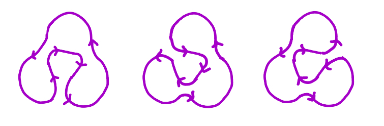
A state $\sigma$ contributes in the state sum only if its global orientation is compatible. For instance, for the right handed trefoil knot the various oriented diagrams with compatible orientations that contribute in the state sum of (97) are shown in Fig. 3.

Figure 3: Various oriented diagrams contributing in the state sum (97) for the trefoil knot (left), along with their coefficients $[\mathcal{K}|\sigma]$.

Note that each configuration corresponding to diagrams in the top row will appear 3 times with the same coefficient, since the same splitting can be applied to any of the 3 crossings of the trefoil (see Fig. 4 for an example).

Figure 4: Three oriented states with the same coefficient $c_{\sigma}(z)=[\mathcal{K}|\sigma]=-z^{3}$.

Hence a total 16 states (out of 27 possibilities) contribute for the trefoil knot.

Using that $\bar{H}(A,z)=A^{-w}R(\mathcal{K};A,z)$ and by setting $A=q^{-1}a^{2},$ $z=q-q^{-1}$ so that $\widetilde{\overline{KF}}(\mathcal{K};q^{-1}a^{2},q-q^{-1})=-(q^{-1}a^{2})^{-w}[\mathcal{K}](ia,q)$, (70) can be written as

$$\hskip-34.1433ptR(q^{-1}a^{2},q-q^{-1})=-\frac{1}{2}([\mathcal{K}](ia,q)-[\mathcal{K}](a,-q))$$ (99)

$$=-\frac{1}{2}\sum_{\sigma}\left(c_{\sigma}(q)\left(\frac{q}{ia}\right)^{{\rm rot}(\sigma)}R_{\sigma}(ia,q)-c_{\sigma}(-q)\left(\frac{-q}{a}\right)^{{\rm rot}(\sigma)}R_{\sigma}(a,-q)\right)$$

which becomes a relation between between the HOMFLY–PT polynomial of the knot and its states. This relation is verified to be true in the case of the trefoil knot, for which the sum over states $\sigma$ in the RHS involves the states presented in Fig. 3.

The Jaeger expansion can also be used to write down a formal character expansion for the Dubrovnik polynomial in terms of the characters of $SU(N)$, i.e. the Schur functions $S_{Q}$, listed in Appendix A. By setting $A=q^{-1}a^{2}$ and $z=q-q^{-1}$, for a knot $\mathcal{K}$ that has a braid representative with $m$ strands and writhe $w$ this can be expressed as

$$\bar{Y}(\mathcal{K};A,z)=(qa^{-2})^{w}\sum_{\sigma}c_{\sigma}(qa^{-1})^{{\rm rot}(\sigma)}\sum_{Q(\sigma)}h^{Q}(\sigma)S_{Q}.$$ (100)

Here the last summation refers to the character expansion corresponding to the state $\sigma$, which usually can be expressed as a braid with less than $m$ strands. For instance, for the 3-stranded unknot $T(3,1)$ we find

$$\hskip-17.07164pt\bar{Y}(T(3,1);a,q)=(1-q^{4}a^{-4})S_{[2]}-q^{-2}(1-q^{4}a^{-4})S_{[11]}$$ (101)

$$\hskip 11.38109pt+q^{3}a^{-3}(1+q^{2}a^{-2})S_{[3]}-qa^{-3}(1+q^{2}a^{-2})S_{[21]}+q^{-1}a^{-3}(1+q^{2}a^{-2})S_{[111]}$$

which simplifies to the standard expression $\bar{Y}(\bigcirc)=\frac{A-A^{-1}}{z}+1$ at $A=q^{-1}a^{2}$ and $z=q-q^{-1}$, as expected.

Although state sums do not provide the most efficient description of the Dubrovnik polynomial and its relation to HOMFLY–PT, as the above examples show, they are still a powerful theoretical tool and hence we include this Appendix here for completeness. An interesting application could be to use the Jaeger’s state sum to derive a homology theory corresponding to the Kauffman polynomial, in an analogous way as the Kauffman bracket (the state sum of the Jones polynomial) led to the Khovanov homology [23].

References

• [1] J.M.F. Labastida and E. Pérez, A relation between the Kauffman and the HOMFLY polynomials for torus knots, J. Math. Phys. 37 (1996) 2013. arXiv:q-alg/9507031.
• [2] A. Petrou and S. Hikami, Harer-Zagier transform of the HOMFLY–PT polynomial for families of twisted hyperbolic knots, J. Phys. A: Math. Theor. 57 (2024) 205204, arXiv: 2307.05919.
• [3] A. Petrou and S. Hikami, The HOMFLY–PT polynomial and HZ factorisation, arXiv: 2412.04933.
• [4] A. Petrou and S. Hikami, Character expansion and the Harer-Zagier transform of knot polynomials, arXiv:2505.10629.
• [5] V. Bouchard, B. Florea and M. Marino, Counting higher genus curves with crosscaps in Calabi-Yau orientifolds, JHEP 0412 (2004) 035, arXiv:hep-th/0405083.
• [6] A. Mironov, A. Morozov, An. Morozov and A. Sleptsov, Gaussian distribution of LMOV numbers, Nucl. Phys. B924 (2017) 1. arXiv: 1706.00761.
• [7] F. Jaeger, p.219 in ”Knot and Physics” [15], (communicated by L.H. Kauffman)
• [8] J.S. Birman and H. Wenzl, Braids, link polynomials and a new algebra, Trans. Am. Math. Soc. 313 (1989) 249.
• [9] J. Murakami, The Kauffman polynomial of links and representation theory, Osaka J. Math. 24 (1987), 745.
• [10] J. Murakami, The representations of the q-analogue of Brauer’s centralizer algebras and the Kauffman polynomial of links, Publ. RIMS, Kyoto Univ. 26 (1990) 935.
• [11] J. Murakami, The parallel version of polynomial invariants of links, Osaka J. Math. 26 (1989) 1.
• [12] E. Brézin, S. Hikami and J. Zinn-Justin, Generalized non-linear $\sigma$-models with gauge invariance, Nucl. Phys. B165 (1980) 528.
• [13] A. Mironov, A. Morozov and And. Morozov, Character expansion for HOMFLY polynomials II: Fundamental representation. Up to five strands in braid. JHEP 03 (2012) 034, arXiv: 1112.2654.
• [14] S. Hikami, Punctures and $p$-spin curves from matrix models III. $D_{l}$ type and logarithmic potential, J. Stat. Phys. 188 (2022) 20. arXiv:2111.13793.
• [15] L.H. Kauffman, Knots and Physics, World Scientific (2001).
• [16] A. Mironov, Mkrtchyan and A. Morozov, On universal knot polynomials, JHEP 02 (2016) 078. arXiv:1510.05884.
• [17] Knot Atlas, http://katlas.org/wiki/Main Page (by D.Bar-Natan)
• [18] S. Stevan, Chern-Simons invariants of torus links, Ann. Henri Poincaré 11 (2010) 1201. arXiv: 1003.2861.
• [19] D.E. Littlewood, Products and plethysms of characters with orthogonal, symplectic and symmetric groups, Canadian Journal of Mathematics, 10 (1958) 17.
• [20] H. Weyl, The classical groups, their invariants and representations, 2nd ed., Princeton Univ. Press, Princeton, N.J. (1946).
• [21] V. Turaev, Faithful linear representations of the braid groups. Asterisque-Societe-Mathematique De France. 276 (2002) 389-410.
• [22] H. Wenzl, Quantum groups and subfactors of type B, C, and D. Commun. Math. Phys. 133, 383–432 (1990). https://doi.org/10.1007/BF02097374
• [23] M. Khovanov, A. Categorification of the Jones polynomial, Duke Math J. 101 (2000) 359, arXiv:math.QA/9908171.
• [24] L.Kauffman and S. Lins, Temperley-Lieb recoupling theory and invariants of 3-manifold, Annals of Math Studies 134 (1994).
• [25] L.H. Kauffman and S.J. Lomonaco Jr., Braiding operators are universal quantum gates, New J. Phys. 6 (2004) 134. arXiv:quant-ph/0401090.
• [26] R. Gopakumar and C. Vafa, M-theory and topological strings-II, arXiv: hep-th/9812127.
• [27] T. Liko and L.H. Kauffman, Knot theory and a physical state of quantum gravity, Class. Quantum Grav. 23 (2006) R63, arXiv:hep-th/0505069.
• [28] W. Fulton and J. Harris, Representation theory, A first course, Chap. 20, Springer (2004).