Extending Neural Operators: Robust Handling of Functions Beyond the Training Set

We develop a rigorous framework for extending neural operators to handle out-of-distribution input functions. We leverage kernel approximation techniques and provide theory for characterizing the input-output function spaces in terms of Reproducing Kernel Hilbert Spaces (RKHSs). We provide theorems on the requirements for reliable extensions and their predicted approximation accuracy. We also establish formal relationships between specific kernel choices and their corresponding Sobolev Native Spaces. This connection further allows the extended neural operators to reliably capture not only function values but also their derivatives. Our methods are empirically validated through the solution of elliptic partial differential equations (PDEs) involving operators on manifolds having point-cloud representations and handling geometric contributions. We report results on key factors impacting the accuracy and computational performance of the extension approaches.

Introduction

Neural operators provide a class of machine learning methods for data-driven learning of mappings between spaces of functions [Bronstein2021, Izenman2012, Stuart2010, Atzberger2022, Atzberger2020, Chen1995, Kovachki2021a]. Examples include learning solution operators for Partial Differential Equations (PDEs) and Integral Operators [Strauss2007, Pozrikidis1992, Audouze2009, AtzbergerQuackenbushGNP2024, Bhattacharya2021], estimators for inverse problems [Stuart2010, Kaipio2006, Gelman1995], estimating geometric quantities [AtzbergerQuackenbushGNP2024, Atzberger2020, Quackenbush2025], and data assimilation [Stuart2010, Asch2016]. Neural operators can be used to provide approaches for non-linear approximations, for learning representations for analytically unknown operations through training, or provide accelerations of frequent operations performed in iterative algorithms [Chui2018, Izenman2012, Meilua2023, Atzberger2020, Atzberger2022, Bronstein2021].

Neural operators use deep neural networks for learning operators by leveraging a lifting operation to featurize an input function and a collection of linear integral operations coupled with non-linear activations. This allows for learning mappings that generalize the discrete finite layers of multi-layer perceptrons and by integration are less sensitive to noise in the input functions and the resolution at which they are sampled [Kovachki2023a].

We perform analysis of neural operators to characterize in more detail the natural function spaces that arise when making different choices for the training data. We provide ways to extend neural operator mappings beyond the functions in the training set by leveraging results in kernel approximation. For judicious choices of the training sets this results in input and output functions spaces corresponding to Reproducing Kernel Hilbert Spaces that can be viewed as embedded within Sobolev Spaces. This allows for developing extensions that not only ensure convergence of the functions but also of their derivatives. We provide theory and theorems that further characterize these spaces and the key factors impacting the accuracy of the extended neural operators.

Some related work has been done on architectural design of neural operators and on the development of theory for their approximation properties in [Lu2022, Le2025, Kovachki2023a, Korolev2022, Pordanesh2025, Mezidi2025, Berner2025, Mezidi2025]. In [Lu2022, Le2025, Kovachki2023a], the approximation capabilities are characterized for classes of operators approximable by neural operator variants. A proof is given of dimension-independent approximation bounds for two-layer networks that provide mappings between Banach spaces in [Korolev2022]. In [Le2025], analysis is performed for the stability and generalization error and neural operators. A few different architectures for neural operators have also been proposed with structures motivated by results in functional analysis in [Pordanesh2025, Mezidi2025, Berner2025]. This includes the development of multi-scale and spectral kernels [Kovachki2023a], unified frameworks for lifting pointwise layers to operator spaces [Berner2025], and the introduction of nonlinear skip connections derived from functional optimization problems to facilitate the training of deeper networks [Mezidi2025].

In our work, we consider alternative approaches and generalize the action of the operators through kernel-based reconstructions instead of relying primarily on data-driven interpolation. Most current methods depend strongly on the distribution of the training data and interpolation to determine out-of-distribution performance. In contrast, we construct an operator extension method based on the native spaces of a collection of training kernels. In previous work, approximation bounds are developed for neural operators [Kovachki2023a, Lu2022] based on general properties. In our work, we provide a more constructive framework that provides more specialized error bounds based on the kernel choice and geometry of the domain. We also address the setting of operators on embedded manifolds, characterizing smoothness penalties that arise when restricting ambient kernels to the embedded geometric domain. This provides more detailed bounds with more problem-specific attributes to control sources of error or to inform architectural and kernel choices.

To complement our theoretical results, we also perform empirical studies showing how the methods perform in practice. This includes investigating learned Laplace-Beltrami operators and how they perform across manifold shapes of varying geometric complexity. For further improvements in computational efficiency, we also introduce an architecture referred to as Separable Geometric Neural Operators (SB-GNPs). We show how our SB-GNPs can be used to perform training which ensures convergence not only of the functions but also their derivatives. This allows for Sobolev training that minimizes the $\mathcal{H}^{1}$ error while maintaining efficiency on large point clouds. We further evaluate our approaches based on approximate Green’s Functions and compare the cases of using (i) Gaussian, (ii) Matérn, and (iii) Wendland kernels. We show that while Gaussian kernels offer high regularity, they induce severe ill-conditioning and poor performance in capturing derivative information. In contrast, we show that Matérn and Wendland kernels provide stable, accurate extensions that control the trade-off between operator approximation and kernel interpolation errors. These provide for ways to obtain more robust methods for extending the neural operators and capturing derivative information for input functions that were not seen in the training data. We further characterize the role of hyper-parameters of these neural operator methods through a collection of benchmark studies.

We organize the paper as follows. We discuss background on neural operators, kernel methods, and our extension approaches in Section 1. We then discuss theory on our operator extensions and the related Reproducing Kernel Hilbert Spaces (RKHSs) in Section 2. We provide proofs of our main theorems in Section 3. We discuss how our approaches can be incorporated in practice into neural operator architectures and ways the training performance can be made more efficient in Section 4. We demonstrate the extension methods in approximating solution operators for geometric PDEs and perform empirical studies to further characterize their accuracy and other properties in Section 5. Our results show a few practical ways neural operators can be extended to handle robustly input functions beyond the training data.

1 Neural Operators

Neural operators are used to learn mappings between function spaces using as training data evaluations from pairs of functions $\left\{(f_{i}(\cdot),u_{i}(\cdot))\right\}_{i=1}^{N}$. For a target operator $u_{i}=\mathcal{G}[f_{i}]$, a neural operator learns an approximate operator $\mathcal{G}_{\theta}$, [Kovachki2021a]. Neural operators are motivated by applications that include speeding up operations during solving inverse problems [Kovachki2023a], accelerating simulations [azizzadenesheli2024neural], approximating solution maps $\mathcal{S}_{\theta}$ for parameteric PDEs [Kovachki2023a, FNO_2020], and geometric tasks involving solving PDEs on manifolds and curvature-driven shape deformations [Quackenbush2025, AtzbergerQuackenbushGNP2024].

We consider neural operators $w=\mathcal{G}_{\theta}[u]$ of the form

$$\mathcal{G}_{\theta}=\mathcal{Q}\circ\sigma_{T}\left(W_{T}+\mathcal{K}_{T}\right)\circ\dots\circ\sigma_{0}\left(W_{0}+\mathcal{K}_{0}\right)\circ\mathcal{P}.$$ (1)

This consists of $T$ layers with the following three learnable components, (i) a lifting operator $\mathcal{P}[a]$ with $a\in\mathbb{R}^{d_{a}}$ where for $a=(\{u(\tilde{x}_{i})\}_{i=1}^{N},\{x_{i}\}_{i=1}^{N})$ a set of features are obtained from the function evaluations to yield $v_{0}\in\mathbb{R}^{d_{v}}$ with $d_{v}\geq d_{a}$, (ii) a composition of layers involving integral operators $\mathcal{K}[v]$ and linear operators $\mathcal{W}[v](x)$ that are processed through a non-linear activation $\sigma_{i}[\cdot]$ to obtain $v_{i+1}=\sigma_{i}\left(Wv_{i}+\mathcal{K}[v_{i}]\right)$, and (iii) a projection operator $\mathcal{Q}$ that gives a $\mathbb{R}^{d_{u}}$-valued output function $w$. The activation of the last layer $\sigma_{T}$ is typically taken to be the identity. The trainable sub-components also include within the operator layers the kernel $\kappa$ and the local function operator $W$. We collect all trainable parameters into $\theta$ for the neural operator $\mathcal{G}_{\theta}$.

For $\mathcal{K}$ we consider integral operators of the form

$$\mathcal{K}[v](x)=\int_{D}\kappa(x,y)v(y)\ d\mu(y).$$ (2)

The $\mu$ is a measure on $D\subset\mathbb{R}^{d_{v}}$, $v:D\to\mathbb{R}^{d_{v}}$ is the input function, and $\kappa$ is the operator kernel $\kappa(x,y)\in\mathbb{R}^{d_{v}}\times\mathbb{R}^{d_{v}}$. In practice, the integral is often approximated on a truncated domain $B_{r}(x)$ using

$$\tilde{\mathcal{K}}[v_{t}](x_{j})=\frac{1}{N}\sum_{x_{k}\in B_{r}(x_{j})}\kappa(x_{j},x_{k})v_{t}(x_{k}).$$ (3)

This discretization can be interpreted as performing message passing on a graph [gilmer2020message, gori2005new]. As further motivation for this work and to illustrate the main ideas for the extensions, we consider the problem of learning operators $u=\mathcal{S}_{\theta}[f]$ to approximate the solutions to a class of PDEs.

1.1 Approximation of Solution Operators for Partial Differential Equations.

Consider the solution operator $u=\mathcal{S}[f]$ for PDEs of the form

$$\mathcal{L}u(x)=f(x),\quad x\in\Omega.$$ (4)

Here, $\Omega$ is a bounded domain and $\mathcal{L}$ is a bounded linear operator with inverse $\mathcal{S}=\mathcal{L}^{-1}$. We consider the case of boundary conditions that are Dirichlet with $u(x)=0$ for $x\in\partial\Omega$ or Neumann $\nabla u(x)\cdot n(x)=0$ with in the latter solutions determined uniquely by also requiring $\int u(x)dx=0$. In the case of kernels $k_{\sigma}:\Omega\times\Omega\to\mathbb{R}$ that are symmetric, positive-definite, and translation invariant, we can express the kernels as $k_{\sigma}(x,y)=\Phi(\sigma(x-y))$. We refer to $\Phi(r)$ as the radial function associated with the kernel $k$. We take the shape factor $\sigma>0$ which controls the length-scale $\ell_{k}=\sigma^{-1}$ over which the kernel varies. The length-scale $\ell_{k}$ is also referred to as the band-width of the kernel. This controls the range of decay of the kernel and in discretizations the band-width of associated matrices.

To train the neural operators $\mathcal{S}_{\theta}$ to approximate solution operators $\mathcal{S}$, we use solutions of the following instances of the problem

$$\mathcal{L}_{x}g_{\sigma}(x,y)=k_{\sigma}(x,y),\quad x,y\in\Omega.$$ (5)

The target solution operator can be expressed as $\mathcal{S}:k_{\sigma}\rightarrow g_{\sigma}$. We use training data
$\left\{(k_{\sigma}(\cdot,x_{i}),g_{\sigma}(\cdot,x_{i}))\right\}_{i=1}^{N}$, where $k_{\sigma}$ serves the role of the input function and $g_{\sigma}$ the target output solution function.

In the case $k_{\sigma}(x,y)$ has compact support and integrates to one, we have in the limit of $\sigma\to\infty$ that the kernel behaves similar to a Dirac $\delta$-function with $k_{\sigma}(x,y)\rightarrow\delta(x-y)$. In this case the $g_{\sigma}$ approximates the Green’s Function $G(x,y)$ for elliptic PDEs of the form of equation 4. Motivated by this, we call $\tilde{g}_{\sigma}(x,y)=\mathcal{S}_{\theta}[k_{\sigma}(x,y)]$ the Pseudo-Green’s Functions of $\mathcal{L}$ with respect to $k_{\sigma}$.

Since solutions to such PDEs can be constructed through super-position using the Green’s Function, this motivates the relationship to functions $f\in\mathcal{H}_{k}(\Omega)$ in the Reproducing Kernel Hilbert Space (RKHS) of $k_{\sigma}$. More generally, we consider functions $f$ in the associated Native Space for the RKHS [Aronszajn1950, berlinet2011reproducing]. For such functions, we can use kernel techniques to obtain approximations of the function $f$ of the form

$$\tilde{f}(x)=\sum_{i=1}^{\left\lvert X\right\rvert}\alpha_{i}k_{\sigma}(x,x_{i}),\quad x_{i}\in X.$$ (6)

The $X\subset\Omega$ is a finite discrete set of points that are used as centers for the kernel evaluations.

For a function $u$ that is a solution to the PDE in equation 4 having as the right-hand-side function $f$, we can use $\tilde{f}$ and the Pseudo-Green’s Functions to obtain the approximate solution

$$\tilde{u}(x)=\sum_{i=1}^{\lvert X\rvert}\alpha_{i}\tilde{g}_{\sigma}(x,x_{i}).$$ (7)

This procedure illustrates a way to obtain an approximate solution mapping $\tilde{\mathcal{S}}:\tilde{f}\rightarrow\tilde{u}$ for the operator $\mathcal{S}$.

As we discuss in more detail below, this allows us to handle a broad class of input functions beyond the training data. The explicit use of kernel approximations allows us more control over the learned operator’s behaviors instead of just relying on the empirical neural network training of interpolation or extrapolation of responses. As we also discuss below, we further can establish theory for the accuracy of our operator extensions and characterize other key factors that contribute to the errors and robustness of the approximations obtained from our training protocols and extension methods.

1.2 Theory for Extending Neural Operators

Figure 1: Operator Extension Methods. We develop methods for extending conventional neural operators and geometric neural operators to robustly handle inputs beyond the functions in the training data. We leverage properties of kernel approximations. Neural operators process an input function $w(\cdot)$ and geometric neural operators also process information from the geometry $\Phi(\cdot)$. The operators use a combination of a featurizing lifting operator $\mathcal{P}$, kernel operator layers, and a projection operator $\mathcal{Q}$ to obtain the output function $u(\cdot)$, (top). We obtain representations for input functions in terms of kernels $k_{\sigma}$, (lower-left). The kernel constructions are shown for a subset of the points in the sum. The operator layer involves a combination of a kernel integration $\mathcal{K}[v]$ and a linear operation ${W}[v]$ that is passed through a non-linear activation function $\sigma(\cdot)$, (lower-center). The kernel representations are then used to construct the output function $\tilde{u}(\cdot)$, (lower-right).

For extending neural operators more generally requires theory to characterize the roles played by the choice of kernel and other factors impacting the accuracy and other properties of the operator. To understand how an extended neural operator will handle inputs beyond the training data also requires determining the input and output function spaces generated by the extensions.

For analysis of the neural operators, we consider a compact set $\Omega\subset\mathbb{R}^{d}$ a symmetric positive-definite kernel $k:\Omega\times\Omega\to\mathbb{R}$ whose native space $\mathcal{H}_{k}(\Omega)$ is equivalent in norm to the Sobolev Space $\mathcal{H}^{s}(\Omega)$, where $\lceil s\rceil>d/2+2$, [brezis2011functional, leoni2017first]. In this setting, for any $f\in\mathcal{H}^{s}(\Omega)$ and $\epsilon>0$, there exists a finite set $X\coloneqq\left\{x_{i}\right\}_{i=1}^{N}\subset\Omega$ and a sequence $\bm{\alpha}$ with $\alpha_{i}=[\bm{\alpha}]_{i}$ such that for any $\epsilon>0$

$$\tilde{f}(x)=\sum_{i=1}^{N}\alpha_{i}k_{\sigma}(x,x_{i})$$ (8)

and satisfies

$$\left\lVert\tilde{f}-f\right\rVert_{\mathcal{H}^{s}(\Omega)}<\epsilon.$$ (9)

In this case, the extended neural operator $\mathcal{S}_{\theta,k}^{e}$ is given by

$$\tilde{u}=\mathcal{S}_{\theta,k}^{e}[f]:=\sum_{i=1}^{|X|}\alpha_{i}\mathcal{S}_{\theta,k}[k_{\sigma}(\cdot,x_{i})].$$ (10)

This uses the learned operator $\mathcal{S}_{\theta,k}$ which was trained only on input functions of the form $k_{\sigma,j}=k_{\sigma}(\cdot,x_{j})$. The steps of the extension method are illustrated in Figure 1.

We establish two theorems on the behaviors and accuracy of the neural operators and our extensions methods, with more details given in Section 3. The first theorem gives a result for neural operator extensions for functions having domain in $\Omega\subset\mathbb{R}^{d}$. The second theorem gives a result for extended geometric neural operators when the functions are defined on a manifold $\Omega=\mathcal{M}$.

We remark that our approaches can be applied most immediately for linear solution operators $\mathcal{S}$. The results also indicate approaches that could further be generalized to other non-linear classes of operators by using kernel representations as part of the lifting/projection operators $\mathcal{P},\mathcal{Q}$ or using alternatives to equation 10 using approaches from functional calculus [haase2018lectures, haase2006functional, reed2012methods]. This also includes using our extension techniques at the single-layer level internally within existing architectures to extend handling of inputs encountered within the internal layer operations.

In the case of neural operators extended for functions having domain in $\Omega\subset\mathbb{R}^{d}$, we have the following result.

Theorem 1.1.

Let $\Omega\subset\mathbb{R}^{d}$ be a compact set and $k(\cdot,\cdot)$ a symmetric positive-definite kernel with a native space that is norm-equivalent to the Sobolev Space $\mathcal{H}^{s}(\Omega)$ for $\lceil s\rceil>d/2+2$. Suppose the operator $\mathcal{S}$ is bounded with $\left\lVert S(f)\right\rVert_{\mathcal{H}^{1}(\Omega)}\leq C_{1}\left\lVert f\right\rVert_{\mathcal{H}^{1}(\Omega)}$. For $\delta>0$ and $\epsilon>0$, suppose the approximating operator $\mathcal{S}_{k,\theta}$ satisfies the uniform bound

$$\left\lVert\mathcal{S}_{k,\theta}[k(\cdot,x)]-\mathcal{S}[k(\cdot,x)]\right\rVert_{\mathcal{H}^{1}(\Omega)}<\delta,\quad x\in\Omega,$$ (11)

and the kernel approximation function $\tilde{f}$ satisfies

$$\left\lVert\tilde{f}-f\right\rVert_{\mathcal{H}^{1}(\Omega)}<\epsilon.$$ (12)

Then, the approximated solution using $\mathcal{S}_{k,\theta}$ and $\tilde{f}$ approximates the true solution to equation 4 with the bound

$$\left\lVert\mathcal{S}_{k,\theta}^{e}[\tilde{f}]-\mathcal{S}[f]\right\rVert_{\mathcal{H}^{1}(\Omega)}\leq C_{1}\epsilon+C_{2}\delta,$$ (13)

where $C_{2}=\left\lVert\bm{\alpha}\right\rVert_{\ell_{1}}$.

We remark that this gives a way to estimate the anticipated accuracy of the extended neural operator $\mathcal{S}^{e}$ given a level of sampling of the domain $X$ and the training accuracy $\delta$. The $C_{1}$ depends on the target operator $S$ and $C_{2}$ depends on the $\ell_{1}$-norm of $\bm{\alpha}$ of the approximating functions $\tilde{f}$. For a set of target functions $\mathcal{F}\subset\mathcal{H}^{s}$, the bound can be used to provide the level of training accuracy $\delta$ needed to ensure accuracy of the extension. The target functions would in practice be application specific where there is often some prior knowledge of characteristic physical scales and other properties. As with any approximation scheme, the more rich the underlying functions the more resolution or analogous information would be required to ensure accurate results. The bounds can be used as part of getting a handle on these requirements for the neural operators used.

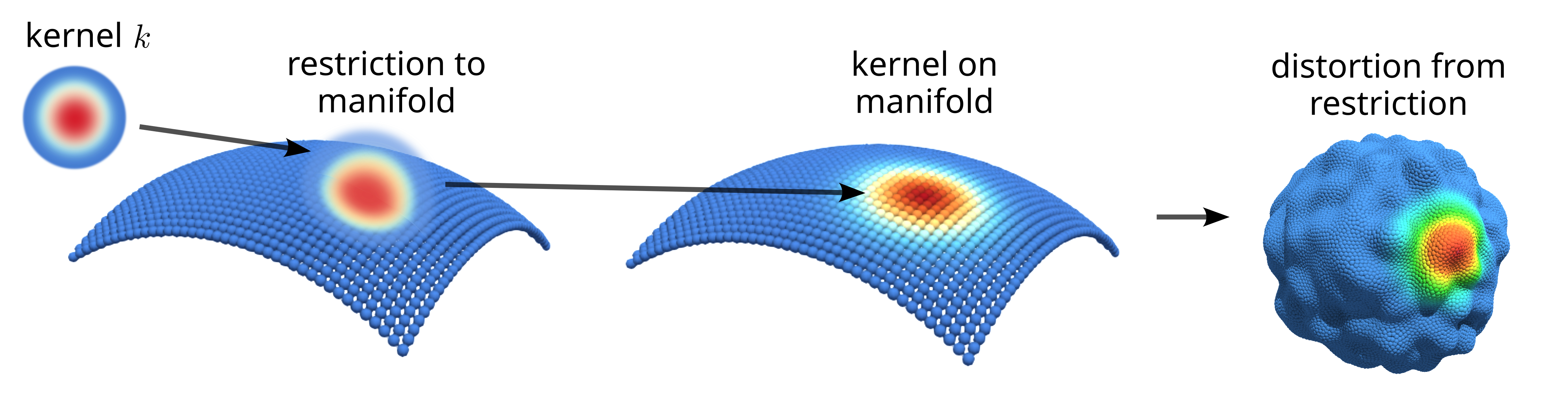
We further develop our results for extending operators on manifolds $\mathcal{M}$. We view these as $m$-dimensional embedded sub-manifolds $\mathcal{M}\subset\mathbb{R}^{d}$ where $m<d$. We use kernels $k_{\mathcal{M}}$ obtained by restricting a kernel $k$ from $\mathbb{R}^{d}$ to $\mathcal{M}$. This gives $k_{\mathcal{M}}:\mathcal{M}\times\mathcal{M}\rightarrow\mathbb{R}$ where we set $k_{\mathcal{M}}(x_{1},x_{2}):=k(x_{1},x_{2})$ with the restriction $x_{1},x_{2}\in\mathcal{M}$. These restricted kernels do not necessarily inherit the properties of $k$. For example, they may no longer be symmetric, translation invariant, or isotropic, see Figure 2. This can impact the approximation properties of the kernels.

For operator extensions in the manifold setting $\Omega=\mathcal{M}$ using restricted kernels $k_{\mathcal{M}}$, we have the following result.

Theorem 1.2.

Let $\mathcal{M}\subset\mathbb{R}^{d}$ be a $m$-dimensional sub-manifold, and let $k:\mathbb{R}^{d}\times\mathbb{R}^{d}\to\mathbb{R}$ be a symmetric positive definite kernel. Consider the kernel $k_{\mathcal{M}}:=k|_{\mathcal{M}}$ obtained by restricting $k$ to the manifold $\mathcal{M}$. For $\delta>0$ and $\epsilon>0$, suppose the approximating operator $\mathcal{S}_{k_{\mathcal{M}},\theta}$ satisfies the uniform bound

$$\left\lVert\mathcal{S}_{k_{\mathcal{M}},\theta}[k_{\mathcal{M}}(\cdot,x)]-\mathcal{S}[k_{\mathcal{M}}](\cdot,x)\right\rVert_{\mathcal{H}^{1}(\mathcal{M})}<\delta,\quad x\in\mathcal{M},$$ (14)

and the $k_{\mathcal{M}}$ kernel approximation of function $\tilde{f}$ satisfies

$$\left\lVert\tilde{f}-f\right\rVert_{\mathcal{H}^{1}(\mathcal{M})}<\epsilon.$$ (15)

If the native space $\mathcal{H}_{k}(\mathbb{R}^{d})$ is norm-equivalent to $\mathcal{H}^{s}(\mathbb{R}^{d})$ with $s-(d-m)/2>m/2$ and $\lceil s-(d-m)/2\rceil\geq 1$, then the following bound holds,

$$\left\lVert\mathcal{S}_{k_{\mathcal{M}},\theta}^{e}[\tilde{f}]-\mathcal{S}[f]\right\rVert_{\mathcal{H}^{1}(\mathcal{M})}\leq C_{1}\epsilon+C_{2}\delta.$$ (16)

These results show how we can extend neural operators in the manifold setting and ensure accuracy in the $\mathcal{H}^{1}$ norm. The Theorem 1.2 also shows to achieve accuracy we can avoid in the manifold setting the cumbersome task of constructing special translation invariant or isotropic kernels on $\mathcal{M}$. We can instead leverage properties of kernels $k$ defined on the ambient space $\mathbb{R}^{d}$ and then restrict them to obtain $k_{\mathcal{M}}$ for $\mathcal{M}$, see Figure 2. These theorems also show for the errors of the extended operators it is sufficient to control the accuracy $\delta$ of the training for the learned operator and the accuracy $\epsilon$ in the kernel approximations. We discuss in more detail below these results and characterize further how the native spaces $\mathcal{H}_{k}(\Omega)$ and $\mathcal{H}_{k}(\mathcal{M})$ depend on the choices for the kernels.

2 Native Spaces for Kernel Approximations.

We consider on $\mathbb{R}^{d}$ kernels $k(\cdot,\cdot)$ that are real-valued, symmetric, positive-definite, and translation invariant. In this case, the kernels can be expressed as $k(x,y)=\Phi(\sigma\cdot(x-y))\in L^{1}(\mathbb{R}^{d})\cap C(\mathbb{R}^{d})$ on $\mathbb{R}^{d}$. For brevity in the notation, we will suppress in many contexts the shape parameter $\sigma$, and take it fixed throughout the discussions. When we are able to use the Fourier transform $\hat{\Phi}$ of $\Phi$, we can characterize the native space $\mathcal{H}_{k}(\mathbb{R}^{d})$ as the collection of functions [Wendland2004]

$$\mathcal{H}_{k}(\mathbb{R}^{d})=\left\{f\in L^{2}(\mathbb{R}^{d})\cap C(\mathbb{R}^{d}):\frac{\hat{f}}{\sqrt{\hat{\Phi}}}\in L^{2}(\mathbb{R}^{d})\right\}.$$ (17)

When $s>d/2$ and

$$\hat{\Phi}(\omega)\sim\left(1+\left\lVert\omega\right\rVert_{2}^{2}\right)^{-s},$$ (18)

we have that the native space $\mathcal{H}_{k}(\mathbb{R}^{d})$ is norm-equivalent to the Sobolev Space $\mathcal{H}^{s}(\mathbb{R}^{d})$ [Santin2018]. The set of kernels that we will consider here can be found in Table 1. This includes the widely-used Gaussian kernel $\Phi(r)=\exp(-r^{2})$. While the Gaussian kernel does not have a native space $\mathcal{H}_{k}$ that is norm-equivalent to any $\mathcal{H}^{s}$, it’s native space is contained as $\mathcal{H}_{k}\subset\mathcal{H}^{s}$ for all positive $s$. This allows us to achieve related error bounds for functions in the native space of Gaussian kernels [Wendland2004].

For manifolds and other geometric structures $\mathcal{M}$, it can be shown that norm equivalence of the native space to Sobolev space also holds provided $\mathcal{M}\subset\mathbb{R}^{d}$ has Lipschitz boundary. In this case, the restriction of $k$ to $\mathcal{M}$ yields the native space $\mathcal{H}_{k}(\mathcal{M})=\mathcal{H}^{s}(\mathcal{M})$, [Wendland2004]. To simplify the notation, we will often denote the domain as $\Omega=\mathcal{M}$ when discussing the manifold case.

Figure 2: Kernels Restricted to Manifolds $k_{\mathcal{M}}$. We develop theory for kernel approximation based on restricting kernels from the bulk ambient space $k(x,y)$ to a manifold surface $k_{\mathcal{M}}(x,y)$. Even when the bulk kernel $k$ has nice properties and symmetries, such as being a radial basis function, the restricted kernels $k_{\mathcal{M}}$ may not inherit these attributes. The $k_{\mathcal{M}}$ may no longer be radial symmetric $k_{\mathcal{M}}(x,y)\neq k_{\mathcal{M}}(|x-y|)$ or translation invariant $k_{\mathcal{M}}(x,y)\neq k_{\mathcal{M}}(x,y+\Delta)$.

We consider $\mathcal{M}$ that are $m$-dimensional embedded smooth sub-manifolds in $\mathbb{R}^{d}$ with $m<d$. We use restricted kernels $\tilde{k}:\mathcal{M}\times\mathcal{M}\to\mathbb{R}$ given by

$$\tilde{k}(x,y)=k_{\mathcal{M}}(x,y)=k|_{\mathcal{M}\times\mathcal{M}}(x,y),\quad x,y\in\mathcal{M}.$$ (19)

In this case, we have the native space $\mathcal{H}_{\tilde{k}}(\mathcal{M})=\mathcal{H}^{s-(d-k)/2}(\mathcal{M})$, [Fuselier2012]. We can see there is a decrease in smoothness which corresponds to a $1/p$ penalty for each co-dimension $d-k$ of the manifold. The most common case we will consider is when $p=2$. This follows from extending trace operators to Sobolev spaces, restricting functions from $\mathbb{R}^{d}$ to $\mathcal{M}$, see [Besov1978]. This is an interesting result since it is what allows for using the kernel $k$ from the embedding space and restricting. This allows us to avoid the potentially cumbersome task of needing to design a kernel intrinsic to the manifold. An example of restricting a kernel $k$ on $\mathbb{R}^{2}$ to a $2$-dimensional manifold can be found in Figure 2.

The results allow for using a wide range of accessible kernels $k$ to generate Sobolev native spaces. This allows our operator extension methods to be applied for a wide set of operators and functions. This also provides results for the accuracy of these methods both for the Euclidean case and the Non-Euclidean manifold setting.

black!20!white Kernel	Radial Function $\bm{\Phi(r)}$	$\bm{\mathcal{H}^{s}(\mathbb{R}^{d})}$	$\bm{\mathcal{H}^{s}(\mathcal{M})}$
black!5!white Gaussian	$\exp\left(-r^{2}\right)$	N/A	N/A
black!12!white Matérn Basic, $\nu=\frac{1}{2}$	$\exp\left(-r\right)$	$s=\frac{d+1}{2}$	$s=\frac{3}{2}$
black!5!white Matérn Linear, $\nu=\frac{3}{2}$	$(1+\sqrt{3}r)e^{-\sqrt{3}r}$	$s=\frac{d+3}{2}$	$s=\frac{5}{2}$
black!12!white Matérn Quadratic, $\nu=\frac{5}{2}$	$(1+\sqrt{5}r+\frac{5}{3}r^{2})e^{-\sqrt{5}r}$	$s=\frac{d+5}{2}$	$s=\frac{7}{2}$
black!5!white Wendland, $k=0$, $l=\lfloor d/2\rfloor+1$	$(1-r)_{+}^{l}$	$s=\frac{d+1}{2}$	$s=\frac{3}{2}$
black!12!white Wendland, $k=1$, $l=\lfloor d/2\rfloor+2$	$(1-r)_{+}^{l+1}((l+1)r+1)$	$s=\frac{d+3}{2}$	$s=\frac{5}{2}$
black!5!white Wendland, $k=2$, $l=\lfloor d/2\rfloor+3$	$(1-r)_{+}^{l+2}((l+1)(l+3)r^{2}+3(l+2)r+3)$	$s=\frac{d+5}{2}$	$s=\frac{7}{2}$

Table 1: Kernels and RKHS Equivalent Native Spaces. For the different kernels $k(x,y)=\Phi(|x-y|)$ and RKHS $\mathcal{H}_{k}$ generated by $k$, we give the equivalent native spaces. In the cases we consider, these are Sobolev spaces $\mathcal{H}^{s}$, [Santin2018]. For an input $\mathbf{x}\in\mathbb{R}^{d}$, we take $r=\left\lVert\mathbf{x}\right\rVert_{2}$. We also consider $\mathbf{x}\in\mathcal{M}$ restricted to a manifold surface $\mathcal{M}\subset\mathbb{R}^{3}$. For kernels obtained by restricting the free-space kernel $k(x,y)$, we also give the corresponding Sobolev space $\mathcal{H}^{s}(\mathcal{M})$.

Figure 3: Kernels. We show a few different kernels used in our approximations and comparison studies. For the Gaussian kernels, we use $\Phi(\sigma\cdot r)$ with values for $\sigma=\ell_{0}^{-1}$ with $\ell_{0}=0.2,0.3,0.4$ for the cases labeled $A$, $B$, $C$. For the Matérn kernels, the $A$, $B$, $C$ cases correspond to the Basic, Linear, and Quadratic kernels with the parameters shown in Table 1. For the Wendland kernels, we consider the cases with $k=0$, $k=1$, $k=2$ with parameters in Table 1.

2.1 Function Approximation using Kernel Methods

For a given kernel $k$ we seek approximations of a function $f$ in the RKHS $\mathcal{H}_{k}$ generated by $k$. We formulate the approximation as the solution to the optimization problem

$$s_{f}^{\lambda}=\operatorname*{arg\,min}_{s\in\mathcal{H}_{k}(\Omega)}\sum_{i=1}^{N}\left(f(x_{i})-s(x_{i})\right)^{2}+\lambda\|s\|_{\mathcal{H}_{k}(\Omega)}.$$ (20)

This gives an approximation for a given set of $N$ points $x_{i}\in X_{N}\subset\Omega$ and given function $f\in\mathcal{H}_{k}(\Omega)$. By the Kernel Representer Theorem any objective function of the form $\ell(s(x_{1}),\ldots,s(x_{N}))+\lambda\|s\|_{\mathcal{H}_{k}}$ always has a minimizing solution of the form $s_{f}^{\lambda}(x)=\sum_{i=1}^{N}\alpha_{i}^{\lambda}k(x,x_{i})$, [Scholkopf2001]. This is useful since it only involves a finite number of kernel evaluations at $x_{i}\in X_{N}$. While in principle there can also be other minimizing functions in $\mathcal{H}_{k}$, we can always achieve the same minimum value of the objective using a function of this form. In our notation, we let $s_{f}=\lim_{\lambda\rightarrow 0}s_{f}^{\lambda}$.

The quality of the function approximation of $s_{f}$ to $f$ depends on the quality of the point sampling $X_{N}$. It can be shown the kernel approximation in equation 20 satisfies at each point $x\in\Omega$ the bound [schaback2023small, Santin2018] with

$$\left\lvert f(x)-s_{f}(x)\right\rvert\leq P_{X_{N}}(x)\left\lVert f\right\rVert_{\mathcal{H}_{k}(\Omega)},\quad x\in\Omega.$$ (21)

The function $P_{X_{N}}$ is called the Power Function of $k$ with respect to $X_{N}$ and can be found using the Newton basis $\left\{l_{i}(x)\in V(X_{N}):l_{i}(x_{j})=\delta_{ij}\right\}$,

$$P_{X_{N}}(x)\coloneqq\left\lVert k(\cdot,x)-\sum_{j=1}^{N}k(\cdot,x_{j})l_{j}(x)\right\rVert_{\mathcal{H}_{k}(\Omega)},\quad x\in\Omega.$$ (22)

The space of functions is defined by $V(X_{N}):=\{h(\cdot)\;|\;h(x)=\sum_{i}\alpha_{i}k(x,x_{i}),\;\;x_{i}\in X_{N}\}$. In practice, while computing $P_{X_{N}}(x)$ is often more difficult than solving the approximation problem, it can provide insights into the key factors impacting approximations. This can be used to obtain bounds on $\left\lvert f(x)-s_{f}(x)\right\rvert$ based on the distribution of the points in $X_{N}$. A useful characteristic is the fill distance $h_{X_{N}}$ of $X_{N}$ defined as

$$h_{X_{N}}\coloneqq\sup_{x\in\Omega}\min_{x_{j}\in X_{N}}\left\lVert x-x_{j}\right\rVert_{2}^{2}.$$ (23)

This can be used in the error analysis of $f(x)$ and $s_{f}(x)$ and their derivatives [Wendland2004]. The $P_{X_{N}}$ depends on the quality of the sampling $X_{N}$. Related to these approaches, we state two theorems below from the literature for the Euclidean $\mathbb{R}^{d}$ setting and the Non-Euclidean embedded sub-manifold $\mathcal{M}$ setting [Wendland2004, Fuselier2012].

Theorem 2.1.

Suppose that $\Omega\subset\mathbb{R}^{d}$ is bounded, has a Lipschitz boundary, and satisfies an interior cone condition. Let $k$ be a positive definite kernel satisfying equation 18 and $\mu\in\mathbb{N}_{0}$ satisfying $\lceil s\rceil-\mu-1>d/2$. Then for any set $X_{N}\subset\Omega$ with $h_{X_{N}}\leq h_{0}$ where $h_{0}$ depends on $s,\Omega$, and any $f\in\mathcal{H}_{k}(\Omega)$, the error between $f$ and its interpolant $s_{f}$ on $X_{N}$ can be bounded by

$$\left\lVert f-s_{f}\right\rVert_{H^{\mu}(\Omega)}\leq Ch_{X_{N}}^{s-\mu}\left\lVert f\right\rVert_{\mathcal{H}^{s}(\Omega)}.$$ (24)

Theorem 2.2.

Let $\mathcal{M}$ be a $m$-dimensional sub-manifold of $\mathbb{R}^{d}$ and $k$ be a positive definite kernel satisfying equation 18, and define $\tilde{k}$ by restricting $k$ to $\mathcal{M}$. Let $\tilde{s}=s-(d-m)/2$, assume $\tilde{s}>m/2$ and let $\mu\in\mathbb{N}$ with $0\leq\mu\leq\lceil\tilde{s}\rceil-1$. Then there is a constant $h_{\mathcal{M}}$ such that if a finite node set $X_{N}\subset\mathcal{M}$ satisfies $h_{X_{N},\mathcal{M}}\leq h_{\mathcal{M}}$, then for all $f\in\mathcal{H}_{\tilde{k}}(\mathcal{M})$ we have

$$\left\lVert f-s_{f}\right\rVert_{\mathcal{H}^{\mu}(\mathcal{M})}\leq Ch_{X_{N},\mathcal{M}}^{\tilde{s}-\mu}\left\lVert f\right\rVert_{\mathcal{H}_{\tilde{k}}(\mathcal{M})}.$$ (25)

The results of Theorem 2.2 show that by using our projected kernels $k_{\mathcal{M}}$ we can still achieve a comparable level of accuracy and convergence as in Theorem 2.1. This provides an approach that gives the same convergence rate as if we had designed an isotropic and translation-invariant kernel for the manifold $\mathcal{M}$. This allows us to construct radial kernels $k$ on the ambient space $\mathbb{R}^{d}$ of dimension $d$ and then by restricting them to obtain $k_{\mathcal{M}}$ still be assured of good approximation properties for the manifold $\mathcal{M}$ of dimension $m$. The $\tilde{s}=s-(d-m)/2$ gives the reduction $d-m$ in smoothness of the Sobolev space with $p=2$ which arises whenever one reduces the spatial dimension of the domain from $d$ to $m$.

The fill distance $h_{X_{N},\mathcal{M}}$ in Theorem 2.2 is with respect to the intrinsic metric $d_{\mathcal{M}}$ of the manifold $\mathcal{M}$. We remark that having the results stated in terms of $h_{X_{N},\mathcal{M}}$ in practice is not an issue since for smooth compact manifolds it can be bounded by the ambient fill distance $h_{X_{N},\mathbb{R}^{d}}$ and these become similar as the density of points increases [Wendland2004, Fuselier2012]. This can also be related to the fill distance considered in the local coordinate charts $h_{X_{N}\cap U_{j},U_{j}}$ for $U_{j}\subset\mathbb{R}^{m}$ [Fuselier2012]. These results can be used to provide bounds for our kernel approximations of functions in our extension methods. It also should be mentioned that in practice the choice of kernel also plays an important role in the level of numerical accuracy and conditioning of the approximations. We discuss in more detail below these and other practical aspects of kernel approximation.

2.2 Function Approximation using Regularized Kernel Methods

The approximations obtained from equation 20 in the limit $\lambda\rightarrow 0$ can become ill-conditioned depending on the choice of kernel and the quality of the point sampling $X_{N}$. The conditioning also tends to become worse as the number of sample points $N$ increases. This can arise from sample points that are nearly identical, overlap of the kernels for points on length-scales smaller than $\sigma^{-1}$, and increasing density as $N$ increases. One approach to mitigate the ill-conditioning is to relax the $\lambda\rightarrow 0$ conditions for residual minimization and instead solve the regularized problem with $\lambda>0$,

$$s_{f}^{\lambda}=\operatorname*{arg\,min}_{s\in\mathcal{H}_{k}(\Omega)}\sum_{i=1}^{N}\left(s(x_{i})-f(x_{i})\right)^{2}+\lambda\left\lVert s\right\rVert_{\mathcal{H}_{k}(\Omega)}^{2}.$$ (26)

The $\lambda$ provides the strength of the regularization. When $\lambda=0$, we recover the residual minimization problem which corresponds to the interpolation case. In practice to find the coefficients of the solution function, we set to zero the gradient of the objective function in equation 26 to obtain the linear problem

$$(A+\lambda I)\bm{\alpha}=\mathbf{b},\quad[\mathbf{b}]_{i}=b_{i}=f(x_{i}),$$ (27)

where $A$ is the Gram Matrix with entries $k(x_{i},x_{j})$ and $\bm{\alpha}$ is the vector of coefficients with $\alpha_{i}=[\bm{\alpha}]_{i}$. When $\lambda>0$ this form of the solution is unique. By adding the regularization term we can ensure that the condition number $\kappa(A+\lambda I)$ satisfies

$$\kappa(A+\lambda I)=\frac{\lambda+\lambda_{\max}(A)}{\lambda+\lambda_{\min}(A)}\leq 1+\lambda_{\max}(A)/\lambda.$$ (28)

This provides a useful bound that no longer depends on the smallest eigenvalue $\lambda_{\min}(A)$. It is known that while the largest eigenvalue has an upper bound of $N\Phi(0)$ that grows according to the number of points, the smallest eigenvalue also can decay rapidly $\rightarrow 0$, [Wendland2004]. The utility of the regularization can be seen since the behavior of the smallest eigenvalue $\lambda_{\min}(A)$ depends on the separation radius $q_{X_{N}}$ defined by

$$q_{X_{N}}\coloneqq\min_{i\neq j}\frac{1}{2}\left\lVert x_{i}-x_{j}\right\rVert_{2}.$$ (29)

This $q_{X_{N}}$ plays a central role in determining how small the eigenvalues become, with $q_{X_{N}}=0$ yielding a zero eigenvalue. For example, in the case of a Gaussian Kernel with $\Phi(r)=\exp(-\sigma r^{2})$, we have the lower bound [Wendland2004]

$$\lambda_{\min}(A)\geq C(2\sigma)^{-d/2}\exp\left(-C^{\prime}/(q_{X_{N}}^{2}\sigma)\right)q_{X_{N}}^{-d}.$$ (30)

While this is a lower bound, for Gaussian kernels this same behavior often occurs for $\lambda_{\min}$ for typical point samplings encountered in applications. In practice, the smallest eigenvalue often decays rapidly toward $0$ as the separation distance $q_{X_{N}}$ becomes small. For a few numerical studies, we show condition numbers in Appendix A. Similar to equation 24, we see a bound in the regularized case also can be obtained of the form [Wendland2005]

$$\left\lVert D^{a}s_{f}^{\lambda}-D^{a}f\right\rVert_{L^{2}(\Omega)}\leq C\left(h_{X_{N}}^{\ell-\left\lvert a\right\rvert}+h_{X_{N}}^{-\left\lvert a\right\rvert}\sqrt{\lambda}\right)\left\lVert f\right\rVert_{\mathcal{H}_{k}(\Omega)}.$$ (31)

The $D^{a}f$ indicates the derivative of the function $f$ with partial derivatives in the $i^{th}$ direction of order $a_{i}=[a]_{i}$. Here, the constant $C>0$ depends on $\Omega,k$ and the smoothness $\ell$ of the kernel. For solving the regularized problem this also suggests balancing the penalty with the fill-distance $h$ by taking $\lambda=\lambda(h)\leq h_{X_{N}}^{2\ell}$. In this case, we obtain the bound

$$\left\lVert s_{f}^{\lambda(h)}-f\right\rVert_{\mathcal{H}^{\left\lvert a\right\rvert}(\Omega)}\leq\tilde{C}h_{X_{N}}^{\ell-\left\lvert a\right\rvert}\left\lVert f\right\rVert_{\mathcal{H}_{k}(\Omega)}.$$ (32)

We remark that this bound holds for the Sobolev-norm $\left\lVert\cdot\right\rVert_{\mathcal{H}^{\left\lvert a\right\rvert}(\Omega)}$ and these results provide ways for us to control the accuracy of the kernel approximation both of functions $f$ and their derivatives $D^{a}f$ in the Native Spaces $\mathcal{H}_{k}$ in terms of the fill-distance $h_{X_{N}}$ of the point samplings $X_{N}$ and choice of kernel $k(\cdot,\cdot)$. As we discuss in more detail and show in our empirical studies, the choice of kernel and parameters can have a significant impact on the performance of the approximations and extension methods.

3 Proofs for the Kernel Extension Theorems 1.1 and 1.2.

We now use the results of the previous sections to provide proofs of our results in Theorem 1.1 and Theorem 1.2. These results leverage the properties of kernel approximation of the input functions. We also utilize the relationship between the Sobolev Native Spaces generated by the unrestricted Euclidean kernels $k(\cdot,\cdot)$ and Non-Euclidean manifold kernels $k_{\mathcal{M}}(\cdot,\cdot)$. We also characterize the behaviors of the associated Sobolev Native Spaces these kernels generate in the manifold setting.

3.1 Proof of Theorem 1.1.

We now establish the bounds given by Theorem 1.1.

Proof.

Fix $\epsilon>0,f\in\mathcal{H}^{s}(\Omega)$, and $\delta>0$. As stated in the theorem, we assume training can be performed to obtain $\mathcal{S}_{k,\theta}$ acting on kernel input functions $k$ having an accuracy $\delta$ for a target operator $\mathcal{S}$ satisfying

$$\left\lVert\mathcal{S}[k(\cdot,x)]-\mathcal{S}_{k,\theta}[k(\cdot,x)]\right\rVert_{\mathcal{H}^{1}(\Omega)}<\delta,\quad x\in\Omega.$$ (33)

Now using Theorem 2.1, we can choose a set of points $X_{N}=\left\{x_{i}\right\}_{i=1}^{N}$ that have a fill distance $h_{X_{N}}$. We choose the fill distance sufficiently small so that $h_{X_{N}}\leq h_{0}$ and

$$h_{X_{N}}^{s-1}<\frac{\epsilon}{C\left\lVert f\right\rVert_{\mathcal{H}^{s}(\Omega)}}.$$ (34)

We use the kernel approximation $s_{f}$ for $f$ that minimizes equation 20. This can be represented as $s_{f}(x)=\sum_{i=1}^{N}\alpha_{i}k(x,x_{i})$ and satisfies $\left\lVert f-s_{f}\right\rVert_{\mathcal{H}^{1}(\Omega)}<\epsilon$ by equation 32 and equation 34. By setting $\tilde{f}=s_{f}$ and using the linearity and boundedness of $\mathcal{S}$, we have

$$\left\lVert\mathcal{S}[f]-\mathcal{S}_{k,\theta}^{e}[s_{f}]\right\rVert_{\mathcal{H}^{1}(\Omega)} \leq \left\lVert\mathcal{S}[f]-\mathcal{S}[s_{f}]\right\rVert_{\mathcal{H}^{1}(\Omega)}+\left\lVert\mathcal{S}[s_{f}]-\mathcal{S}_{k,\theta}^{e}[s_{f}]\right\rVert_{\mathcal{H}^{1}(\Omega)}$$ (35)

$$\leq \left\lVert\mathcal{S}\right\rVert_{\mathcal{H}^{1}(\Omega)}\left\lVert f-s_{f}\right\rVert_{\mathcal{H}^{1}(\Omega)}+\left\lVert\sum_{i=1}^{N}\alpha_{i}(\mathcal{S}-\mathcal{S}_{k,\theta})[k(\cdot,x_{i})]\right\rVert_{\mathcal{H}^{1}(\Omega)}$$ (36)

$$\leq \left\lVert\mathcal{S}\right\rVert_{\mathcal{H}^{1}(\Omega)}\left\lVert f-s_{f}\right\rVert_{\mathcal{H}^{1}(\Omega)}+\sum_{i=1}^{N}\left\lvert\alpha_{i}\right\rvert\left\lVert(\mathcal{S}-\mathcal{S}_{k,\theta})[k(\cdot,x_{i})]\right\rVert_{\mathcal{H}^{1}(\Omega)}$$ (37)

$$\leq C_{1}\epsilon+C_{2}\delta.$$ (38)

The constants are given by $C_{1}=\left\lVert\mathcal{S}\right\rVert_{\mathcal{H}^{1}(\Omega)}$ and $C_{2}=\left\lVert\alpha\right\rVert_{\ell_{1}}=\sum_{i=1}^{N}|\alpha_{i}|$. We obtain equation 35 from the triangle inequality, and equation 36 by using boundedness of $\mathcal{S}$ and the specific form of $\tilde{f}$. We then obtain equation 37 by properties of the norm. The final bound in equation 38 follows from the approximation accuracy of $\tilde{f}$ in equation 12 and the uniform accuracy of $\mathcal{S}_{k,\theta}$ from equation 11. This provides the bound on the accuracy of the operator extension $\mathcal{S}_{k,\theta}^{e}$ given in equation 13. ∎

3.2 Proof of Theorem 1.2.

We next discuss how to prove Theorem 1.2. This requires we obtain estimates when restricting approximations to the sub-manifold $\mathcal{M}$. While there are similarities to the Euclidean case, the restrictions result in kernels that are no longer radial symmetric $k(x,y)\neq k(|x-y|)$ or satisfy the translation invariance properties $k(\cdot,y)\neq k(\cdot,y+\Delta)$ for all $x,y$. The approximations also now only involve sample points from the sub-manifold $x_{i}\in\mathcal{M}$. As part of handling these issues, we leverage Theorem 2.2. We use $s_{f}$ to approximate functions $f$ on $\mathcal{M}$ by minimizing equation 20. From Theorem 2.2, we have the bound

$$\left\lVert f-s_{f}\right\rVert_{H^{\mu}(\mathcal{M})}\leq Ch_{X,\mathcal{M}}^{s-\mu-(d-m)/2}\left\lVert f\right\rVert_{\mathcal{H}^{s-(d-m)/2}(\mathcal{M})}.$$ (39)

We use these results in establishing Theorem 1.2.

Proof.

From equation 25, we obtain $\|\tilde{f}-f\|_{\mathcal{H}^{1}(\mathcal{M})}<\epsilon$ by considering the case when $\mu=1$ with $\tilde{f}=s_{f}$ when the fill-distance $h_{X_{N},\mathcal{M}}$ for points $X_{N}\subset\mathcal{M}$ satisfies

$$h_{X_{N},\mathcal{M}}^{s-(d-m)/2-1}<\frac{\epsilon}{C\left\lVert f\right\rVert_{\mathcal{H}_{\tilde{k}}(\mathcal{M})}}.$$ (40)

We remark that a significant difference with the previous result in equation 34 is that the exponent is augmented now to $s-(d-m)/2$. The $d-m$ is the co-dimension of the sub-manifold $\mathcal{M}$ when embedded in $\mathbb{R}^{d}$. This arises from the distortions that can occur in the kernel approximations when they are restricted to the lower dimensional sub-manifold, as proven in [Fuselier2012].

From these considerations and using the linearity and boundedness of $\mathcal{S}$, we obtain

$$\left\lVert\mathcal{S}[f]-\mathcal{S}_{k,\theta}^{e}[s_{f}]\right\rVert_{\mathcal{H}^{1}(\mathcal{M})} \leq \left\lVert\mathcal{S}[f]-\mathcal{S}[s_{f}]\right\rVert_{\mathcal{H}^{1}(\mathcal{M})}+\left\lVert\mathcal{S}[s_{f}]-\mathcal{S}_{k,\theta}^{e}[s_{f}]\right\rVert_{\mathcal{H}^{1}(\mathcal{M})}$$ (41)

$$\leq \left\lVert\mathcal{S}\right\rVert_{\mathcal{H}^{1}(\mathcal{M})}\left\lVert f-s_{f}\right\rVert_{\mathcal{H}^{1}(\mathcal{M})}+\left\lVert\sum_{i=1}^{N}\alpha_{i}(\mathcal{S}-\mathcal{S}_{k,\theta})[k(\cdot,x_{i})]\right\rVert_{\mathcal{H}^{1}(\mathcal{M})}$$ (42)

$$\leq \left\lVert\mathcal{S}\right\rVert_{\mathcal{H}^{1}(\mathcal{M})}\left\lVert f-s_{f}\right\rVert_{\mathcal{H}^{1}(\mathcal{M})}+\sum_{i=1}^{N}\left\lvert\alpha_{i}\right\rvert\left\lVert(\mathcal{S}-\mathcal{S}_{k,\theta})[k(\cdot,x_{i})]\right\rVert_{\mathcal{H}^{1}(\mathcal{M})}$$ (43)

$$\leq C_{1}\epsilon+C_{2}\delta.$$ (44)

The equation 41 is obtained from the triangle inequality. We obtain the equation 42 by using boundness of the operator $\mathcal{S}$ and the specific form of $\tilde{f}=s_{f}$. This yields equation 43 by properties of the $\mathcal{H}^{1}$ norm. We next use the approximation accuracy of $\tilde{f}$ on the sub-manifold given by equation 15 and the uniform accuracy of $\mathcal{S}_{k,\theta}$ from equation 14. Together, this yields the final equation 44. The constants are given by $C_{1}=\left\lVert\mathcal{S}\right\rVert_{\mathcal{H}^{1}(\mathcal{M})}$ and $C_{2}=\left\lVert\alpha\right\rVert_{\ell_{1}}=\sum_{i=1}^{N}|\alpha_{i}|$. This provides the bound on the accuracy of the operator extension given in equation 16.

∎

This shows that the errors can be controlled for how well the restricted kernels $k_{\mathcal{M}}$ approximate the functions $f$ on the $m$-dimensional sub-manifold $\mathcal{M}$. The operator extensions can achieve accuracy provided we can get the errors sufficiently small in training for the operator responses to $k_{\mathcal{M}}(\cdot,x_{i})$ for $x_{i}\in X_{N}\subset\mathcal{M}$. The main difference with the Euclidean case is the increased need for smoothness in the unrestricted kernel, which is reduced under restriction. We also need sufficiently small manifold fill-distance $h_{X_{N},\mathcal{M}}$. The theory shows that for sufficiently accurate training on kernel responses we can obtain accurate operator extensions for more general functions in the kernel’s native space both in the Euclidean and Non-Euclidean settings. We next discuss in more detail practical ways to obtain effective training methods.

4 Training Methods for the Neural Operators and Sobolev Loss

We discuss how the neural operators can be trained using loss functions based on Sobolev norms. This ensures the training methods result in neural operators that capture both the target functions and their derivatives. This allows for further regularizing the smoothness of the learned operators and helps ensure that physically-relevant information is retained during training. To train our neural operators more efficiently, we also introduce approximations for the kernel integral operators and ways to leverage separable factorizations.

4.1 Approximating Kernel Integral Operators using Separable Factors.

A major computational expense both during training and evaluation of neural operators is computing the kernel integral operators $\mathcal{K}[v]$. For these approximations, edge-based convolutions are widely used to approximate the integrals in equation 2. To improve performance, we develop more efficient alternatives using node-based convolutions by factoring kernels into separable forms.

Consider how a neural operator transforms vector-valued functions $v_{j}(x)$ at the $j$-th layer of an $L$-layer network. The neural operator uses a pointwise linear function represented by a learned matrix $W_{j}$ and a learned kernel $k_{\theta,j}$ processed by a pointwise non-linear activation function $\sigma(\cdot)$. This is performed using the mapping

$$v_{j}(x)\mapsto\sigma\left(W_{j}v_{j}(x)+\int_{\mathcal{D}}\kappa_{\theta,j}(x,y)v_{j}(y)\ dy\right).$$ (45)

The kernel integral is computed on a domain $\mathcal{D}$. In our neural operators, the domain is a ball of radius $r$ giving $\mathcal{D}=B_{r}(x)$. A common method to approximate the integral is to use the edge-based message passing approach

$$\int_{\mathcal{D}}\kappa_{\theta}(x,y)v(y)\ dy\approx\frac{1}{\left\lvert\mathcal{N}(x)\right\rvert}\sum_{y\in\mathcal{N}(x)}\kappa_{\theta}(x,y)v(y).$$ (46)

The $\mathcal{N}(x)$ is the neighborhood of $x$ in the graph constructed with edges between all points at distances less than $r$ from $x$. As the number of points grow, computing equation 46 at every point can become prohibitively expensive both in compute memory and compute time. We introduced in our previous work a few ways to mitigate this by restricting the form and output of the kernels $\kappa_{\theta}$ [AtzbergerQuackenbushGNP2024, Quackenbush2025]. Here, we introduce further approaches for reducing these computational costs.

Figure 4: Kernel Integration: Methods for Improving Performance. In neural operators a major computational cost during both training and evaluation is to compute the kernel integral operations $\mathcal{K}[v]$. An edge-conditioned convolution is widely used for this approximation, but scales as $O(N^{2})$ becoming prohibitively expensive as the density of points increases within the support of the kernel, (top). We develop more computationally efficient alternatives using node-conditioned convolutions based on factoring kernels into a separable form $k(x,y)=k_{1}(x)k_{2}(y)$. The node-based methods scale as $O(N)$ allowing for approximations using efficient gathering and scattering operations greatly reducing computational costs, (bottom).

To simplify the message passing in equation 46, we consider here how to use separable representations of the kernel network by factoring it as $k_{\theta}(x,y)=k_{\theta}^{(1)}(x)k_{\theta}^{(2)}(y)$. We find that this can be used to significantly reduce the costs to obtain more scalable node-conditioned gather-scatter operations. Since there is no longer an explicit dependence on the edge attributes, there are fewer compute steps and the methods are more amenable to parallelization. We also find that our separable architecture allows for training and evaluation on significantly larger point clouds without the need for sub-sampling edges in the graph, further improving accuracy and computational performance.

In more detail, the node-based message passing approach provides better scaling as the number of points $N$ grows. Each kernel network $k^{(i)}_{\theta}$ for $i=1,2$ need only be evaluated $O(N)$ times per layer. On the other hand, in the edge-based approach, the kernel $k_{\theta}$ must evaluate on the edges which grows as $O(N^{2})$. In particular, for the point-cloud resolutions we later consider in Section 5 with $N_{\text{train}}=5000,N_{\text{test}}=10000$, the edge-based convolution methods are so memory intensive we can not even perform the computation for the Sobolev training with an Nvidia A40 GPU. We also find when evaluating the node-based kernel using $N_{\text{test}}$ points takes 160ms compared to the edge-based case taking 2400ms on an Nvidia A40 GPU. Consistent with the asymptotic scaling in $N$, these tests further show the impact of the factorizations on the empirical efficiency gains. The evaluation above already shows a reduction in the computational time of more than $10\times$. As we show below and discuss in more detail, our separable neural operators are still able to achieve comparable accuracy to our previous edge-based results in [AtzbergerQuackenbushGNP2024]. The separable architectures allow for processing larger point-clouds, improve the efficiency of training, and speed up for pre-trained models the evaluation times for neural operators applied to new input functions.

4.2 Sobolev Training of the Neural Operators

In our training of neural operators $\mathcal{G}_{\theta}$, we also consider the accuracy of the derivatives of the output functions by introducing Sobolev norms in the loss function. In the neural operators $\mathcal{G}_{\theta}$, we use within the first $L-1$ layers our separable kernel operators. These layers process the coordinates $x$ along with the function values $f(x)$ based on

$$v_{j}(x,f(x))\mapsto\sigma\left(W_{j}v_{j}(x,f(x))+k_{\theta,1}(x,f(x))\int_{\mathcal{D}}k_{\theta,2}(y,f(y))v_{j}(y,f(y))\ dy\right).$$ (47)

This serves to encode the input function $f$ at the given points $x$. At the final operator layer $L$, we only process the coordinate data $x$ and omit the pointwise linear layer and activation, as also done in [Li2024a].

During training, $\mathcal{G}_{\theta}$ learns to map $f(\cdot)\mapsto u(\cdot)$ for functions on the manifold $\mathcal{M}$. The $u$ is the solution for the PDE having input $f$ in equation 4. To help ensure that $\mathcal{G}_{\theta}$ also learns the surface gradients in the embedding space coordinates, we also incorporate gradients in the loss as

$$\mathcal{L}_{train}(u,\tilde{u})=\frac{\left\lVert u-\tilde{u}\right\rVert_{2}}{\left\lVert u\right\rVert_{2}}+\frac{\left\lVert\nabla_{\mathcal{M}}u-\nabla_{\mathcal{M}}\tilde{u}\right\rVert_{2}}{\left\lVert\nabla_{\mathcal{M}}u\right\rVert_{2}}.$$ (48)

We compute the surface gradients

$$\nabla_{\mathcal{M}}u:=\frac{\partial u}{\partial x^{i}}g^{ij}\mathbf{e}_{j}.$$ (49)

This uses the local coordinate system $\mathbf{x}=(x_{1},x_{2})$ for the surface parameterization $\sigma(x_{1},x_{2})$ with $\mathbf{e}_{j}=\partial_{j}\sigma(x_{1},x_{2})$. This also uses the local inverse metric tensor $g^{-1}$ with components $g^{ij}$. The $\mathbf{e}_{j}$ give the tangent vectors providing a local coordinate basis.

To compute the derivatives of $u$ we use a pointwise operator network $\mathcal{Q}_{\theta}$. This performs a projection of a function to the desired co-domain to obtain $\tilde{u}(x)$

$$\tilde{u}(x)=\mathcal{Q}_{\theta}\left(k_{\theta,L}^{(1)}(x)\int_{\mathcal{D}}k_{\theta,L}^{(2)}(y)v_{L-1}(y,f(y))\ dy\right).$$ (50)

Derivatives can be computed efficiently using automatic differentiation since these only involve the networks $\mathcal{Q}_{\theta}$ and $k_{\theta,L}^{(1)}(x)$.

We further perform a change of basis to represent functions in the embedding space coordinates of $\mathbb{R}^{3}$. For training data, a local basis $\mathbf{e}_{j}$ and geometric quantities then can be computed locally using Generalized Moving Least Squares (GMLS) [Atzberger2020, AtzbergerFPT2022, mirzaei2012generalized]. Since GMLS uses a linear change of coordinates to form a local basis at each point, the gradients computed from $\mathcal{G}_{\theta}$ can be easily transformed to the local chart of the training data when computing equation 49. As we show below, our separable architectures for the neural operators perform well with comparable accuracy to our previous edge-based operator results in [AtzbergerQuackenbushGNP2024]. These architectures allow for significant computational reductions in cost both during training and evaluation of the learned operators on input functions.

5 Results: Accuracy of the Neural Operators and Extension Methods

We demonstrate the methods for empirically approximating the solution operators for geometric PDEs on manifolds. This requires the neural operators to extract from the input functions and geometry the information relevant in constructing the solution functions. We show how our operator extension methods can be used to obtain solution predictions from input functions beyond those encountered during training.

Figure 5: Manifold Shapes and Kernel Restrictions. We show the manifolds used in our comparison studies. We also show how the Wendland kernel with parameter $k=0$ behaves when restricted to the manifold surface to obtain $k_{\mathcal{M}}$. During training the different kernels are centered at a sampling of locations $\{x_{i}\}$ on the manifold providing a collection of functions $k_{\sigma}(\cdot,x_{i})$ for use during training.

We consider the geometric elliptic PDE given by the Laplace-Beltrami equation

$$\begin{cases}\Delta_{\text{LB}}\ u(\mathbf{x})&=-f(\mathbf{x}),\\ \int_{\mathcal{M}}u(\bm{x})\,d\bm{x}&=0,\end{cases}$$ (51)

where

$$\Delta_{LB}=\frac{1}{\sqrt{\left\lvert g\right\rvert}}\partial_{i}\left(g^{ij}\sqrt{\left\lvert g\right\rvert}\partial_{j}\right).$$ (52)

The $\Delta_{LB}$ generalizes the Laplacian to scalar functions on surfaces $\mathcal{M}$. The metric tensor is $g$ with components $g_{ij}$ and the inverse metric tensor $g^{-1}$ with components $g^{ij}$. The determinant of the metric is denoted by $|g|$. The partial derivatives are taken with respect to the directions of the local coordinate system at $x$. For more details, see [Pressley2010, abraham2012manifolds]. We perform studies by considering three radial manifolds $A,B,C$ with shapes having different levels of complexity as shown in Figure 5. We use our operator extension methods discussed in Section 1 and Figure 1. We use our methods to learn an approximation of the solution operator $u=\mathcal{S}[f]$ for equation 51. We train using kernel evaluations $k(\cdot,x_{i})$ to obtain the learned operator $\mathcal{S}_{k,\theta}$ and use our methods to extend this to the operator $\mathcal{S}_{k,\theta}^{e}$ in Section 1 for input functions from the RKHS generated by $k(\cdot,\cdot)$. In our empirical and computational studies, we use throughout the separable factorizations for the kernel operations as discussed in Section 4.

In more detail, we train our neural operators by consider a training set of functions of the form $k_{\sigma}(\cdot,x_{i})$ for kernel responses with $x_{i}$ coming from a fixed subset of points $X_{N}\subset\mathcal{M}$. Once training is complete, we extend our neural operators by using our kernel approximation approach in Section 1 to obtain $\tilde{f}$ of $f$ using the regularized optimization problem given in equation 27 with $\lambda=10^{-10}$. We use the learned neural operator $\mathcal{S}_{k,\theta}$ and our kernel methods to obtain the approximate solution $\tilde{u}(x)=\sum_{i=1}^{N}\alpha_{i}\mathcal{S}_{k,\theta}(k)(x,x_{i})$. This extends the neural operator $\mathcal{S}_{k,\theta}$ trained only on kernel functions $k_{\sigma}(\cdot,x_{i})$ to the more general class of functions $f\in\mathcal{H}_{k}$ in the RKHS $\mathcal{H}_{k}$ generated by $k$. This gives the extended neural operator $\mathcal{S}_{k,\theta}^{e}$.

To obtain $\mathcal{S}_{k,\theta}$ for each choice of kernel $k(\cdot,\cdot)$ and manifold $\mathcal{M}$, we train the neural operator to map $k(\cdot,x_{i})\to\mathcal{S}[k(\cdot,x_{i})]$ using $200$ training pairs of functions $\left\{(k(\cdot,x_{i}),\mathcal{S}[k(\cdot,x_{i})]\right\}$ evaluated at $N_{\text{train}}=10,000$ points. During training, we use Farthest Point Sampling (FPS) to subsample $5,000$ out of $N_{\text{train}}$ points and evaluate the loss in equation 48. All our models consist of $10$ layers and use for the activation function the Gaussian Error Linear Unit (GELU) [Hendrycks2016]. Each kernel network consists of layer widths $(d_{in},w/4,w/2,w,d_{v}^{2})$, use latent dimension $d_{v}=64$ and use width $w=256$. The input dimension $d_{\text{in}}$ is $4$ for the first $9$ layers and $3$ in the final layer, as described in Section 4. All training is performed for $300$ epochs with an initial learning rate $1e-04$ that is halved every $50$ epochs.

During operator evaluation, we use approximations based on equation 27 with $X_{N}$ using $N=1,250$, $2,500$, $5,000$, and $10,000$ points. We compute the relative Sobolev $\mathcal{H}^{1}$ error between the true solution $u(x)$ and the pseudo-Green’s function approximant $\tilde{u}$ at $10,000$ points. We remark that this error includes both the function evaluations and the derivatives. Our ability to train at a resolution of $5,000$ points and test on $10,000$ points is made possible by the approximate discretization invariance properties of our neural operators. Our neural operators have the property that we can train at one level of spatial resolution for the discretizations and evaluate for new functions at other spatial resolutions. For each translation invariant kernel, we consider two different values for the shape parameter $\sigma$ with $k(x,y)=\Phi\left(\sigma\left(x-y\right)\right)$. For Gaussian and Matérn ($\nu=\tfrac{1}{2},\tfrac{3}{2},\tfrac{5}{2}$) kernels, we use $\sigma=5,10$. For the Wendland Kernels of order $k=0,1,2$, we use $\sigma=\tfrac{5}{3},\tfrac{10}{3}$ so that all kernels have comparable support.

We use functions for testing that are generated using band-limited spherical harmonics. For each of the manifolds, we use right-hand side source functions in equation 51 that are generated building on our previous work on spherical harmonics approaches, geometric PDE solvers, and the sphericart Python package [sphericart, Atzberger2018b, sigurdsson2016hydrodynamic, rower2023coarse]. For each function, coefficients were sampled from a normal distribution with standard deviation inversely proportional to the order squared of the spherical harmonic up to a specified maximal degree. The maximal degrees used were $3,6,8,10,12,15,18,22$. We also used $5$ functions for each maximal degree.

black!20!white Kernel	Shape $\bm{\sigma}$	$\bm{N=1250}$	$\bm{2500}$	$\bm{5000}$	$\bm{10000}$
black!20!white Manifold $A$
black!5!white Gaussian	10	2.16e-01	2.18e-01	6.69e-01	7.76e+00
black!5!white Gaussian	5	2.80e+03	1.85e+04	2.80e+04	4.26e+04
black!5!white Matérn, $\nu=1/2$	10	1.14e-01	1.04e-01	1.02e-01	1.02e-01
black!5!white Matérn, $\nu=1/2$	5	1.52e-01	1.53e-01	1.54e-01	1.54e-01
black!5!white Matérn, $\nu=3/2$	10	6.48e-02	6.29e-02	6.27e-02	6.27e-02
black!5!white Matérn, $\nu=3/2$	5	1.04e-01	1.05e-01	1.05e-01	1.05e-01
black!5!white Matérn, $\nu=5/2$	10	7.51e-02	7.48e-02	7.48e-02	7.48e-02
black!5!white Matérn, $\nu=5/2$	5	8.57e-02	8.62e-02	8.62e-02	8.62e-02
black!5!white Wendland, $k=0$	10/3	3.27e-01	3.24e-01	3.23e-01	3.23e-01
black!5!white Wendland, $k=0$	5/3	3.67e-01	3.70e-01	3.71e-01	3.72e-01
black!5!white Wendland, $k=1$	10/3	2.28e-01	2.27e-01	2.27e-01	2.27e-01
black!5!white Wendland, $k=1$	5/3	9.07e-02	9.20e-02	9.23e-02	9.23e-02
black!5!white Wendland, $k=2$	10/3	5.67e-02	5.64e-02	5.65e-02	5.65e-02
black!5!white Wendland, $k=2$	5/3	7.62e-02	7.72e-02	7.72e-02	7.72e-02
black!20!white Manifold $B$
black!5!white Gaussian	10	8.04e-02	8.37e-02	9.14e-01	8.38e+00
black!5!white Gaussian	5	2.04e+01	2.12e+03	3.87e+03	5.80e+03
black!5!white Matérn, $\nu=1/2$	10	5.82e-01	5.79e-01	5.78e-01	5.77e-01
black!5!white Matérn, $\nu=1/2$	5	1.29e-01	1.31e-01	1.32e-01	1.33e-01
black!5!white Matérn, $\nu=3/2$	10	1.19e-01	1.19e-01	1.19e-01	1.19e-01
black!5!white Matérn, $\nu=3/2$	5	1.47e-01	1.47e-01	1.48e-01	1.48e-01
black!5!white Matérn, $\nu=5/2$	10	9.42e-02	9.35e-02	9.35e-02	9.34e-02
black!5!white Matérn, $\nu=5/2$	5	1.16e-01	1.17e-01	1.17e-01	1.17e-01
black!5!white Wendland, $k=0$	10/3	9.75e-02	8.84e-02	8.68e-02	8.65e-02
black!5!white Wendland, $k=0$	5/3	9.52e-02	9.78e-02	9.92e-02	9.97e-02
black!5!white Wendland, $k=1$	10/3	2.66e-01	2.65e-01	2.65e-01	2.65e-01
black!5!white Wendland, $k=1$	5/3	9.68e-02	9.79e-02	9.81e-02	9.82e-02
black!5!white Wendland, $k=2$	10/3	8.29e-02	8.24e-02	8.25e-02	8.25e-02
black!5!white Wendland, $k=2$	5/3	9.47e-02	9.62e-02	9.63e-02	9.63e-02
black!20!white Manifold $C$
black!5!white Gaussian	10	1.54e-01	1.55e-01	1.92e-01	3.44e+00
black!5!white Gaussian	5	3.16e+00	1.74e+02	1.86e+03	2.88e+03
black!5!white Matérn, $\nu=1/2$	10	1.45e-01	1.35e-01	1.32e-01	1.32e-01
black!5!white Matérn, $\nu=1/2$	5	1.41e-01	1.42e-01	1.43e-01	1.43e-01
black!5!white Matérn, $\nu=3/2$	10	1.18e-01	1.17e-01	1.17e-01	1.17e-01
black!5!white Matérn, $\nu=3/2$	5	1.40e-01	1.41e-01	1.41e-01	1.41e-01
black!5!white Matérn, $\nu=5/2$	10	1.12e-01	1.12e-01	1.12e-01	1.12e-01
black!5!white Matérn, $\nu=5/2$	5	1.62e-01	1.64e-01	1.65e-01	1.66e-01
black!5!white Wendland, $k=0$	10/3	1.66e-01	1.59e-01	1.58e-01	1.58e-01
black!5!white Wendland, $k=0$	5/3	1.42e-01	1.44e-01	1.46e-01	1.46e-01
black!5!white Wendland, $k=1$	10/3	1.49e-01	1.47e-01	1.47e-01	1.47e-01
black!5!white Wendland, $k=1$	5/3	1.42e-01	1.47e-01	1.49e-01	1.49e-01
black!5!white Wendland, $k=2$	10/3	1.14e-01	1.13e-01	1.13e-01	1.13e-01
black!5!white Wendland, $k=2$	5/3	1.32e-01	1.42e-01	1.46e-01	1.48e-01

Table 2: Relative $\bm{\mathcal{H}^{1}}$-norm Accuracy. We show results for the accuracy of the extended neural operators when used to obtain solutions of equation 51. We show in bold all relative errors above $10^{0}$. The Gaussian kernels are found to perform poorly as $N$ increases. The extension methods using the Matérn and Wendland kernels are found to perform well as $N$ increases.

We study the relative accuracy in the $\mathcal{H}^{1}$-norm for our extended neural operator predictions of solution functions $\tilde{u}$ for the geometric PDE in equation 7. We report values for each manifold-kernel pair averaged over all test functions in Table 2. We find the Gaussian kernels perform significantly worse than the Matérn and Wendland kernels. As part of our empirical studies when solving equation 27 with $N$ kernel points, we track the $\ell^{1}$-norm of the coefficients $\left\{\alpha_{i}\right\}$ in equation 6. The $\ell^{1}$-norm contributes to the error estimate through the term $C_{2}$ in Theorems 1.1 in equation 1.2. We report these results in Table 3.

We find in the case of the Matérn and Wendland kernels that the $\left\lVert\alpha\right\rVert_{\ell^{1}}$ is on the order of $10^{3}$ or less. These kernels maintain a similar order of magnitude as $N$ increases. In contrast for Gaussian kernels, the $\left\lVert\alpha\right\rVert_{\ell^{1}}$ increases dramatically as $N$ increases. This appears to be related to the well-known ill-conditioning of the Gram matrix $K$ for Gaussian kernels as the separation radius of the point sampling decreases. Additional discussions of the general theory of stability of kernel methods can be found in [Wendland2004]. We present condition numbers for all Gram matrices used our studies in Appendix A.

Our results show there is a significant impact of the ill-conditioning of the Gaussian kernel which greatly amplifies the error in the learned pseudo-Green’s functions. This degrades for Gaussians as the amount of overlap between kernel functions increases. We see this is most pronounced when the kernel has a larger support as the $\sigma$ value becomes smaller, see Table 2.

We find when solving equation 27 the Matérn kernels exhibit significantly better conditioning in $K$ than Gaussian kernels. This results in better approximation when super-imposing the pseudo-Green’s functions. Further, we see in almost all cases that for the Matérn kernels there is more consistency exhibited when varying the number of kernel points $N$ when solving equation 27. For the manifold $A$, all errors vary between $6\%$ and $15\%$ and exhibit better approximation when taking $\sigma=10$. The lowest error of $6.3\%$ occurs when $\nu=3/2$. The manifold $B$ also generally shows better results when $\sigma=10$ with errors varying between $9\%$ and $15\%$ with the exception of $\nu=1/2$. When $\nu=1/2$ and $\sigma=10$, we find the larger $\mathcal{H}^{1}$ errors are a result of inaccurate gradient approximations during training, see discussions in Appendix A. The increase in errors for the manifold $C$ is somewhat expected since it has a more complicated shape and geometric variations. However, despite this we still see our methods are able to achieve consistent results between $11\%$ and $17\%$ error. We also remark that the trends across all manifolds for the Matérn kernel show better results for $\sigma=10$ and $\nu>1/2$.

Wendland kernels differ from the Matérn and Gaussian kernels by having compact support vanishing outside a ball of radius $r$. In practice, this results in efficiencies in evaluation and even better conditioning in the Gram matrix $K$ especially when compared to the Gaussian kernels [Wendland2004]. As a consequence of Wendland kernel’s compact support, our neural operator training methods are variable due to the lack of signal at locations outside of the kernel support. We see this when evaluating on the manifolds $A$, $B$, particularly when $k<2$. Despite this, we still see strong performance for order $k=2$ across all three manifolds, which attains for manifolds $A,B,C$ errors of $5.7\%$, $8.3\%$, and $11.4\%$.

Our results show the trade-offs that occur between the choice of kernel type, hyper-parameters, and geometry. Our studies further show choosing a kernel with smaller support (larger $\sigma$) enables better conditioning of the Gram Matrix which in turn reduces the upper bound $C_{2}$ in Theorem 1.1 and Theorem 1.2. We also find if $\sigma$ is too large this can lead to difficulties in training for the GNPs, as would occur also for other neural operators and kernel methods. Further, we find choosing smoother kernels with good conditioning such as the Matérn ($\nu=5/2)$ or Wendland ($k=2$) kernels achieves a good balance yielding the best results across all three test manifolds $A,B,C$, see Table 2. These results show the importance of using alternatives to Gaussian kernels to obtain good performance.

black!20!white Kernel	Shape $\bm{\sigma}$	$\bm{N=1250}$	$\bm{2500}$	$\bm{5000}$	$\bm{10000}$
black!5!white Gaussian	10	1.34e+03	6.65e+03	6.32e+05	2.05e+07
black!5!white Gaussian	5	2.05e+08	3.08e+09	6.84e+09	1.13e+10
black!5!white Matérn, $\nu=1/2$	10	1.28e+03	1.49e+03	1.59e+03	1.63e+03
black!5!white Matérn, $\nu=1/2$	5	1.53e+03	1.79e+03	1.91e+03	1.96e+03
black!5!white Matérn, $\nu=3/2$	10	1.17e+03	1.26e+03	1.30e+03	1.32e+03
black!5!white Matérn, $\nu=3/2$	5	2.26e+03	2.57e+03	2.77e+03	2.89e+03
black!5!white Matérn, $\nu=5/2$	10	1.15e+03	1.25e+03	1.34e+03	1.46e+03
black!5!white Matérn, $\nu=5/2$	5	3.64e+03	4.87e+03	6.58e+03	8.43e+03
black!5!white Wendland, $k=0$	10/3	1.21e+03	1.36e+03	1.43e+03	1.47e+03
black!5!white Wendland, $k=0$	5/3	1.96e+03	2.31e+03	2.47e+03	2.55e+03
black!5!white Wendland, $k=1$	10/3	1.22e+03	1.31e+03	1.38e+03	1.43e+03
black!5!white Wendland, $k=1$	5/3	3.38e+03	3.98e+03	4.41e+03	4.67e+03
black!5!white Wendland, $k=2$	10/3	4.64e+02	4.95e+02	5.52e+02	6.25e+02
black!5!white Wendland, $k=2$	5/3	1.26e+03	1.94e+03	2.88e+03	3.93e+03

Table 3: Coefficient $\bm{\ell^{1}}$-norms and $\bm{C_{2}}$. We show the $\|\alpha\|_{\ell^{1}}$ of the coefficients $\{\alpha_{i}\}$ in equation 6 when solving equation 27. Results are averaged over all functions and manifolds. This gives an indication of the size of $C_{2}=\|\alpha\|_{\ell^{1}}$ in the accuracy bounds in Theorem 1.2 in equation 16. We highlight in bold all values larger than $10^{4}$. As the number of sample points increases, we see the Gaussian kernels have especially large values exceeding those of our other kernels by a few orders of magnitude. Relative to the other kernels, this indicates using Gaussians in the extension methods could be inefficient and sensitive to the accuracy of the trained neural operators, see equation 16.

Conclusions

We have shown how learned neural operators can be refined for enhanced robustness and improved generalization to out-of-distribution input functions. By leveraging kernel approximation techniques, we achieve well-controlled responses across a broad range of functions beyond those encountered in the training data. We show that selecting kernels corresponding to Reproducing Kernel Hilbert Spaces (RKHSs) associated with Sobolev spaces enables learned operators and extensions to capture mappings of both functions and their derivatives. Beyond our methodological contributions, we establish a theoretical framework to characterize the approximation accuracy and identify key error factors. This includes the critical roles played by the point sampling, kernel type, and kernel bandwidth. The practical utility of the methods was validated through applications for solving elliptic PDEs, operators on manifolds having point-cloud representations, and handling geometric contributions. The methods offer systematic approaches for empirically controlling and extending neural operators for diverse learning tasks.

Appendix A Additional Results: Role of Kernel Choices and Sources of Error

We present additional results on the condition number of the Gram matrix for the various kernels and resolutions prior to adding any regularization when solving equation 27. These results are shown in in Table 4. Our results especially highlight well-known ill-conditioning phenomenon that can arise when using Gaussian kernels. Our results further show how Matérn and Wendland kernels can be used to obtain much better conditioning for systems. We also show how the condition number grows with the number of points $N$ and the impact of the smoothness parameters $\nu$ and $k$, see Table 4.

We also show results for the relative $L^{2}$-errors for $\tilde{u}$ and $\nabla\tilde{u}$ in Tables A and A. We find in our studies that nearly all of the relative errors in Table A are below 10%. This highlights that the majority of the contributions to the $\mathcal{H}^{1}$ error in Table 2 arise from errors in approximating the gradient $\nabla u$. For the Gaussian kernel case, we see again signs of the ill-conditioning arising even in the error for the functions $u$. This becomes increasingly an issue for Gaussian kernels as $N$ becomes large when approximating the the source function $f$. These errors then propagate through the other calculations in the Gaussian kernel case, see Tables A and A.

In summary, our studies and results further highlight the importance of the choice of the radial kernel functions used in our extension methods and for training neural operators more generally. When using alternative kernels, such as the Matérn and Wendland kernels we find much better performance both in capturing the functions $u$ and even in some cases their derivatives.

black!20!white Kernel	Shape $\bm{\sigma}$	$\bm{N=1250}$	$\bm{2500}$	$\bm{5000}$	$\bm{10000}$
black!5!white Gaussian	10	1.07e+03	7.45e+05	3.99e+11	6.36e+19
black!5!white Gaussian	5	1.21e+10	5.36e+18	1.19e+20	1.23e+21
black!5!white Matérn, $\nu=1/2$	10	1.61e+01	4.33e+01	1.34e+02	3.59e+02
black!5!white Matérn, $\nu=1/2$	5	1.19e+02	3.36e+02	1.07e+03	2.84e+03
black!5!white Matérn, $\nu=3/2$	10	3.72e+01	1.77e+02	1.25e+03	6.01e+03
black!5!white Matérn, $\nu=3/2$	5	8.81e+02	4.82e+03	3.73e+04	1.83e+05
black!5!white Matérn, $\nu=5/2$	10	6.43e+01	4.83e+02	7.11e+03	6.14e+04
black!5!white Matérn, $\nu=5/2$	5	4.12e+03	4.22e+04	7.61e+05	7.06e+06
black!5!white Wendland, $k=0$	10/3	1.76e+01	4.90e+01	1.55e+02	4.16e+02
black!5!white Wendland, $k=0$	5/3	1.33e+02	3.77e+02	1.19e+03	3.21e+03
black!5!white Wendland, $k=1$	10/3	4.27e+01	2.33e+02	1.82e+03	9.03e+03
black!5!white Wendland, $k=1$	5/3	1.21e+03	6.93e+03	5.51e+04	2.74e+05
black!5!white Wendland, $k=2$	10/3	3.27e+01	3.36e+02	6.29e+03	5.95e+04
black!5!white Wendland, $k=2$	5/3	3.32e+03	3.81e+04	7.36e+05	7.05e+06

Table 4: Condition Numbers for the Gram Matrix. We show results for the Gram Matrix $K_{ij}=k(x_{i},x_{j})$ for the Gaussian, Matérn, and Wendland kernels. We highlight in bold conditions numbers larger than $10^{6}$. We find as $N$ increases the Gaussian kernels produce particularly ill-conditioned gram matrices which are orders of magnitude larger than the other kernels. The condition numbers are seen to grow much more slowly for the Matérn and Wendland kernels. The larger condition numbers can be seen to correspond to the less accurate cases in Table 3. These results further highlight importance of the choice of kernel when using the extension methods.

black!20!white Kernel	Shape $\bm{\sigma}$	$\bm{N=1250}$	$\bm{2500}$	$\bm{5000}$	$\bm{10000}$
black!20!white Manifold $A$
black!5!white Gaussian	10	1.10e-01	1.11e-01	5.02e-01	5.13e+00
black!5!white Gaussian	5	1.79e+03	1.25e+04	1.94e+04	2.99e+04
black!5!white Matérn, $\nu=1/2$	10	6.09e-02	4.50e-02	4.26e-02	4.24e-02
black!5!white Matérn, $\nu=1/2$	5	5.37e-02	5.45e-02	5.52e-02	5.55e-02
black!5!white Matérn, $\nu=3/2$	10	2.93e-02	2.81e-02	2.83e-02	2.83e-02
black!5!white Matérn, $\nu=3/2$	5	3.85e-02	3.90e-02	3.92e-02	3.92e-02
black!5!white Matérn, $\nu=5/2$	10	3.13e-02	3.12e-02	3.13e-02	3.13e-02
black!5!white Matérn, $\nu=5/2$	5	4.73e-02	4.77e-02	4.77e-02	4.77e-02
black!5!white Wendland, $k=0$	10/3	2.12e-01	2.08e-01	2.07e-01	2.07e-01
black!5!white Wendland, $k=0$	5/3	6.11e-02	6.43e-02	6.58e-02	6.64e-02
black!5!white Wendland, $k=1$	10/3	9.18e-02	9.17e-02	9.18e-02	9.18e-02
black!5!white Wendland, $k=1$	5/3	4.94e-02	5.08e-02	5.11e-02	5.11e-02
black!5!white Wendland, $k=2$	10/3	2.81e-02	3.07e-02	3.11e-02	3.11e-02
black!5!white Wendland, $k=2$	5/3	3.30e-02	3.33e-02	3.33e-02	3.33e-02
black!20!white Manifold $B$
black!5!white Gaussian	10	2.77e-02	2.92e-02	3.75e-01	3.88e+00
black!5!white Gaussian	5	1.15e+01	1.27e+03	2.25e+03	3.44e+03
black!5!white Matérn, $\nu=1/2$	10	7.51e-02	6.11e-02	5.82e-02	5.77e-02
black!5!white Matérn, $\nu=1/2$	5	5.57e-02	5.78e-02	5.85e-02	5.88e-02
black!5!white Matérn, $\nu=3/2$	10	3.34e-02	3.16e-02	3.15e-02	3.15e-02
black!5!white Matérn, $\nu=3/2$	5	5.64e-02	5.75e-02	5.76e-02	5.76e-02
black!5!white Matérn, $\nu=5/2$	10	2.79e-02	2.77e-02	2.78e-02	2.78e-02
black!5!white Matérn, $\nu=5/2$	5	6.06e-02	6.16e-02	6.17e-02	6.18e-02
black!5!white black!5!white Wendland, $k=0$						10/3	4.95e-02	3.28e-02	2.96e-02	2.92e-02
black!5!white Wendland, $k=0$	5/3	5.09e-02	5.41e-02	5.55e-02	5.60e-02
black!5!white Wendland, $k=1$	10/3	6.35e-02	6.55e-02	6.60e-02	6.61e-02
black!5!white Wendland, $k=1$	5/3	4.87e-02	4.99e-02	5.01e-02	5.02e-02
black!5!white Wendland, $k=2$	10/3	2.71e-02	2.78e-02	2.80e-02	2.81e-02
black!5!white Wendland, $k=2$	5/3	3.88e-02	3.97e-02	4.00e-02	4.00e-02
black!20!white Manifold $C$
black!5!white Gaussian	10	3.62e-02	4.33e-02	1.05e-01	2.97e+00
black!5!white Gaussian	5	1.54e+00	7.43e+01	7.33e+02	1.16e+03
black!5!white Matérn, $\nu=1/2$	10	5.86e-02	4.03e-02	3.79e-02	3.79e-02
black!5!white Matérn, $\nu=1/2$	5	5.93e-02	6.38e-02	6.60e-02	6.69e-02
black!5!white Matérn, $\nu=3/2$	10	3.59e-02	3.46e-02	3.51e-02	3.53e-02
black!5!white Matérn, $\nu=3/2$	5	6.81e-02	7.12e-02	7.22e-02	7.25e-02
black!5!white Matérn, $\nu=5/2$	10	3.54e-02	3.38e-02	3.37e-02	3.37e-02
black!5!white Matérn, $\nu=5/2$	5	8.02e-02	8.72e-02	8.98e-02	9.07e-02
black!5!white Wendland, $k=0$	10/3	6.07e-02	4.70e-02	4.60e-02	4.64e-02
black!5!white Wendland, $k=0$	5/3	6.43e-02	7.01e-02	7.31e-02	7.42e-02
black!5!white Wendland, $k=1$	10/3	4.74e-02	4.28e-02	4.23e-02	4.21e-02
black!5!white Wendland, $k=1$	5/3	6.73e-02	7.71e-02	8.07e-02	8.18e-02
black!5!white Wendland, $k=2$	10/3	3.06e-02	2.61e-02	2.58e-02	2.57e-02
black!5!white Wendland, $k=2$	5/3	6.25e-02	8.14e-02	8.82e-02	9.04e-02

Table 5: $\bm{L^{2}}$-norm Relative Errors for $\bm{\tilde{u}}$. We show the accuracy of approximating $\bm{\tilde{u}}$ when solving equation 27. We show in bold errors larger than $1.0$. The accuracy of these results indicates that the main source of error in the Sobolev-norm in Table 2 likely arises from approximation of the gradients. We report these results in Table A.

black!20!white Kernel	Shape $\bm{\sigma}$	$\bm{N=1250}$	$\bm{2500}$	$\bm{5000}$	$\bm{10000}$
black!20!white Manifold $A$
black!5!white Gaussian	10	2.42e-01	2.44e-01	7.18e-01	8.43e+00
black!5!white Gaussian	5	3.04e+03	2.01e+04	3.03e+04	4.61e+04
black!5!white Matérn, $\nu=1/2$	10	1.27e-01	1.16e-01	1.15e-01	1.15e-01
black!5!white Matérn, $\nu=1/2$	5	1.70e-01	1.72e-01	1.73e-01	1.73e-01
black!5!white Matérn, $\nu=3/2$	10	7.25e-02	7.05e-02	7.03e-02	7.03e-02
black!5!white Matérn, $\nu=3/2$	5	1.17e-01	1.17e-01	1.17e-01	1.17e-01
black!5!white Matérn, $\nu=5/2$	10	8.43e-02	8.40e-02	8.39e-02	8.39e-02
black!5!white Matérn, $\nu=5/2$	5	9.45e-02	9.51e-02	9.51e-02	9.51e-02
black!5!white Wendland, $k=0$	10/3	3.59e-01	3.56e-01	3.55e-01	3.55e-01
black!5!white Wendland, $k=0$	5/3	4.20e-01	4.23e-01	4.24e-01	4.25e-01
black!5!white Wendland, $k=1$	10/3	2.59e-01	2.57e-01	2.57e-01	2.57e-01
black!5!white Wendland, $k=1$	5/3	1.00e-01	1.02e-01	1.02e-01	1.02e-01
black!5!white Wendland, $k=2$	10/3	6.34e-02	6.27e-02	6.27e-02	6.27e-02
black!5!white Wendland, $k=2$	5/3	8.50e-02	8.62e-02	8.62e-02	8.62e-02
black!20!white Manifold $B$
black!5!white Gaussian	10	9.18e-02	9.54e-02	1.02e+00	9.32e+00
black!5!white Gaussian	5	2.23e+01	2.31e+03	4.22e+03	6.32e+03
black!5!white Matérn, $\nu=1/2$	10	6.76e-01	6.73e-01	6.72e-01	6.71e-01
black!5!white Matérn, $\nu=1/2$	5	1.45e-01	1.47e-01	1.48e-01	1.49e-01
black!5!white Matérn, $\nu=3/2$	10	1.37e-01	1.36e-01	1.36e-01	1.36e-01
black!5!white Matérn, $\nu=3/2$	5	1.66e-01	1.66e-01	1.66e-01	1.67e-01
black!5!white Matérn, $\nu=5/2$	10	1.08e-01	1.07e-01	1.07e-01	1.07e-01
black!5!white Matérn, $\nu=5/2$	5	1.29e-01	1.30e-01	1.30e-01	1.30e-01
black!5!white black!5!white Wendland, $k=0$						10/3	1.09e-01	1.01e-01	9.91e-02	9.88e-02
black!5!white Wendland, $k=0$	5/3	1.06e-01	1.08e-01	1.10e-01	1.10e-01
black!5!white Wendland, $k=1$	10/3	3.07e-01	3.06e-01	3.05e-01	3.05e-01
black!5!white Wendland, $k=1$	5/3	1.08e-01	1.09e-01	1.09e-01	1.09e-01
black!5!white Wendland, $k=2$	10/3	9.49e-02	9.43e-02	9.43e-02	9.43e-02
black!5!white Wendland, $k=2$	5/3	1.07e-01	1.09e-01	1.09e-01	1.09e-01
black!20!white Manifold $C$
black!5!white Gaussian	10	1.79e-01	1.80e-01	2.15e-01	3.61e+00
black!5!white Gaussian	5	3.60e+00	2.00e+02	2.15e+03	3.33e+03
black!5!white Matérn, $\nu=1/2$	10	1.66e-01	1.56e-01	1.53e-01	1.53e-01
black!5!white Matérn, $\nu=1/2$	5	1.61e-01	1.61e-01	1.61e-01	1.62e-01
black!5!white Matérn, $\nu=3/2$	10	1.36e-01	1.35e-01	1.35e-01	1.35e-01
black!5!white Matérn, $\nu=3/2$	5	1.58e-01	1.59e-01	1.59e-01	1.59e-01
black!5!white Matérn, $\nu=5/2$	10	1.29e-01	1.29e-01	1.29e-01	1.29e-01
black!5!white Matérn, $\nu=5/2$	5	1.82e-01	1.84e-01	1.85e-01	1.85e-01
black!5!white Wendland, $k=0$	10/3	1.90e-01	1.84e-01	1.83e-01	1.83e-01
black!5!white Wendland, $k=0$	5/3	1.61e-01	1.63e-01	1.64e-01	1.64e-01
black!5!white Wendland, $k=1$	10/3	1.72e-01	1.70e-01	1.70e-01	1.70e-01
black!5!white Wendland, $k=1$	5/3	1.61e-01	1.65e-01	1.67e-01	1.67e-01
black!5!white Wendland, $k=2$	10/3	1.33e-01	1.32e-01	1.32e-01	1.32e-01
black!5!white Wendland, $k=2$	5/3	1.50e-01	1.59e-01	1.63e-01	1.64e-01

Table 6: $\bm{L^{2}}$-norm Relative Errors for $\bm{\nabla\tilde{u}}$. We show the accuracy of approximating $\nabla\tilde{u}$ when solving equation 27. We show in bold errors larger than $1.0$. The accuracy of these results indicates that the gradients are the dominant source of approximation error in the Sobolev-norm in Table 2.