Non-Invasive Reconstruction of Intracranial EEG Across the Deep Temporal Lobe from Scalp EEG based on Conditional Normalizing Flow

Abstract

Although obtaining deep brain activity from non-invasive scalp electroencephalography (EEG) is crucial for neuroscience and clinical diagnosis, directly generating high-fidelity intracranial electroencephalography (iEEG) signals remains a largely unexplored field, limiting our understanding of deep brain dynamics. Current research primarily focuses on traditional signal processing or source localization methods, which struggle to capture the complex waveforms and random characteristics of iEEG. To address this critical challenge, this paper introduces NeuroFlowNet, a novel cross-modal generative framework that reconstructs iEEG signals from scalp EEG over multiple medial temporal lobe (MTL) subregions covered by depth microelectrodes in a public synchronized EEG–iEEG dataset. NeuroFlowNet is built on Conditional Normalizing Flow (CNF), which directly models complex conditional probability distributions through reversible transformations, thereby explicitly capturing the randomness of brain signals and fundamentally avoiding the pattern collapse issues common in existing generative models. Additionally, the model integrates a multi-scale architecture and self-attention mechanisms to robustly capture fine-grained temporal details and long-range dependencies. Validation on a publicly available synchronized EEG-iEEG dataset shows that NeuroFlowNet can generate band-limited iEEG signals that closely match the ground truth in the time domain, reproduce low-/mid-frequency spectral characteristics (0.5-50 Hz, including the alpha band 8-13 Hz), and preserve the inter-channel correlation structure underlying MTL functional connectivity. Moreover, compared with representative deterministic regression baselines under the same subject-specific protocol, NeuroFlowNet yields consistently lower errors in the inter-channel correlation matrix, indicating improved functional-connectivity fidelity. These results support the feasibility of non-invasive iEEG reconstruction over the recorded MTL subregions, offering a practical route toward studying deep-brain dynamics from scalp EEG under a subject-specific setting. The code of this study is available in https://github.com/hdy6438/NeuroFlowNet

[1]organization=School of Artificial Intelligence, Chongqing University of Technology, city=Chongqing, postcode=400054, country=China

[2]organization=School of Smart Health, Chongqing Polytechnic University of Electronic Technology, city=Chongqing, postcode=401331, country=China

1 Introduction

Electroencephalography (EEG) is a high-time-resolution brain activity monitoring technique that can track neuronal activation in real time and dynamically record brain activity. It plays a crucial role in brain-computer interfaces, clinical diagnosis, and cognitive neuroscience research [15, 38, 33, 40]. Among these, scalp electroencephalography (EEG) measures the distribution of potentials on the scalp resulting from the propagation of postsynaptic potentials and action potentials from neuronal clusters in the brain, as detected by electrodes placed on the scalp [43, 40]. It offers the advantages of simplicity and high flexibility, making it widely used in clinical monitoring and diagnosis [8]. However, due to the influence of cranial volume conduction effects during signal propagation, its spatial resolution is relatively low [20, 21, 33, 65, 24]. That is, the measured signals represent the superimposed potentials formed by the activities of numerous sources within the brain on the scalp surface. These signals are characterized by weak potentials, susceptibility to external noise interference, and low signal-to-noise ratios, making it difficult to accurately decode the complex dynamic relationships of deep brain neural activities [42, 45]. This limitation restricts its further application in clinical settings. In contrast, intracranial electroencephalography (iEEG) can directly obtain neural activity signals from the cerebral cortex or deep nuclei, featuring high temporal-spatial resolution and high signal-to-noise ratio [47]. It is the gold standard for locating lesions in brain-related diseases and achieving high-precision neural decoding [48, 44]. However, its high surgical costs and the risks of immune reactions and infections following electrode implantation significantly limit its practical application [48].

Given the limited spatial resolution of EEG and the difficulty in obtaining iEEG signals, the brain electroencephalogram inverse problem has emerged as a research hotspot to achieve real-time monitoring and precise localization of neuronal activity [18, 7, 6]. Its core lies in how to infer the spatial distribution and temporal information of cortical and deep neuronal electrical activity from EEG signals recorded on the scalp [18, 43]. By solving the EEG inverse problem, it is possible to map non-invasive EEG signals to neural signals of approximately iEEG quality [57, 26]. This not only helps to “unlock” dynamic information from deep brain regions under non-invasive conditions [22] but also provides new technical support for precise localization of epileptic foci, analysis of brain functional mechanisms, and neural rehabilitation interventions [55].

However, significant differences in discharge patterns and signal characteristics between EEG and iEEG limit the effectiveness of traditional methods [53, 27]. Parameter-based localization methods based on equivalent current dipoles (ECD) are constrained by the difficulty in accurately estimating the number of dipoles [43, 59], while source reconstruction methods based on current distribution are hindered by discrepancies between prior constraints and actual neuronal activity [36], both of which struggle to accurately reconstruct complex neural dynamics [51, 16]. Additionally, traditional machine learning methods rely on manual feature extraction [54, 19] and have limited nonlinear modeling capabilities [54], further restricting their representation capabilities in EEG inversion.

In recent years, deep learning techniques have significantly improved EEG inversion performance through their powerful nonlinear fitting capabilities [52, 12, 31]. For example, convolutional neural networks (CNNs) extract spatial correlations between multiple channels through spatial convolution, enhancing the accuracy of source space imaging [25, 30, 35]. Recurrent neural networks (RNNs) and their variants can model the temporal dynamic characteristics of signals, significantly improving the ability to distinguish between transient and sustained source activity [11, 56]. However, deep learning methods still face numerous challenges. Due to data limitations, model training often relies on large-scale synthetic data generated using finite element or boundary element models [17]. Synthetic data struggles to fully reflect the true complex mapping relationship between EEG and deep neuronal electrical activity, severely limiting the model’s performance in real clinical applications. Additionally, the outputs of this method are primarily continuous neural activity distribution maps, which can locate positions but struggle to capture neural response waveforms, thereby impacting further decoding analysis [14].

Generative models offer a new approach for high-fidelity mapping from EEG signals to iEEG signals, with the core mechanism being the use of generative networks to perform cross-modal conversion of easily obtainable non-invasive EEG signals into iEEG signals. Abdi-Sargezeh et al. were the first to introduce generative adversarial networks (GANs) to address this issue [1], successfully generating high-quality iEEG waveforms while demonstrating advantages in terms of efficiency and model complexity. Building on this, they proposed an EEG-to-EEG conversion model, named VAE-cGAN [2], combining variational autoencoders (VAE) and conditional generative adversarial networks (cGAN), and validated it on a dataset containing real iEEG signals recorded via Foramen Ovale electrodes. By encoding EEG into the latent space and regenerating iEEG signals, they further enhanced the fidelity and signal resolution of the mapped waveforms. The team achieved waveform reconstruction for the first time under conditions where real iEEG was used as a reference, providing a new technical pathway for non-invasive acquisition of high-fidelity iEEG signals. However, this research remains in its preliminary exploratory phase. Due to limitations such as the sampling range of Foramen Ovale channels and inherent defects like mode collapse in GAN models, current reconstruction is only feasible for localized regions of the medial temporal lobe (MTL), and expanding the number of reconstruction channels may significantly degrade reconstruction quality and effectiveness. Additionally, expanding the number of reconstructed channels may significantly degrade reconstruction quality and effectiveness. Additionally, due to the complexity and randomness of neural activity in the brain, models like GAN and VAE, which use deterministic mappings, often fail to adequately reflect the spatiotemporal diversity and randomness of iEEG signals. In addition to waveform fidelity, a fundamental requirement for iEEG reconstruction is to preserve the multi-channel dependency structure across intracranial contacts, since functional connectivity analyses are typically derived from inter-channel covariance/correlation patterns [13, 62]. In an EEG-to-iEEG setting, the inverse mapping is underconstrained: multiple intracranial configurations can be compatible with similar scalp observations due to volume conduction and source mixing. Deterministic regressors trained with pointwise objectives may therefore converge to “average” solutions that reduce waveform error but attenuate network-level variability and distort the inter-channel correlation matrix.

To address these challenges, this study innovatively proposes a new cross-modal generative framework named NeuroFlowNet, which attempts for the first time to reconstruct iEEG signals across multiple MTL subregions using EEG. To capture the spatio-temporal diversity and randomness of iEEG signals, the model is based on Conditional Normalizing Flow (CNF), directly learning the complex conditional probability distribution $p(X_{iEEG}|X_{EEG})$ from EEG to iEEG. Compared to traditional deterministic mappings, the normalizing flow model precisely maps complex data distributions to simple prior distributions (such as Gaussian distributions) through a series of reversible transformations, enabling the generation of more diverse and probabilistically realistic iEEG samples. This effectively addresses the issue of existing methods ignoring the inherent randomness of brain activity and avoids the pattern collapse phenomenon that may occur during model training. Additionally, the model adopts a multi-scale architecture combined with self-attention mechanisms, further enhancing the fineness and robustness of iEEG waveform reconstruction. NeuroFlowNet has been validated for effectiveness on a publicly available dataset [9] of whole temporal lobe EEG-iEEG signals synchronously collected via Stereoelectroencephalography electrodes. Experimental results demonstrate that the model has advantages in signal fidelity, spectral feature reproduction, and network structure recovery. This provides a more precise and reliable new paradigm for non-invasive analysis of deep brain dynamics.

2 Methods

Figure 1: Overview of NeuroFlowNet architecture. The model consists of multiple scales, each containing a series of flow steps that transform the iEEG data conditioned on the EEG data. The final latent variable $Z$ is obtained by concatenating the outputs from all scales.

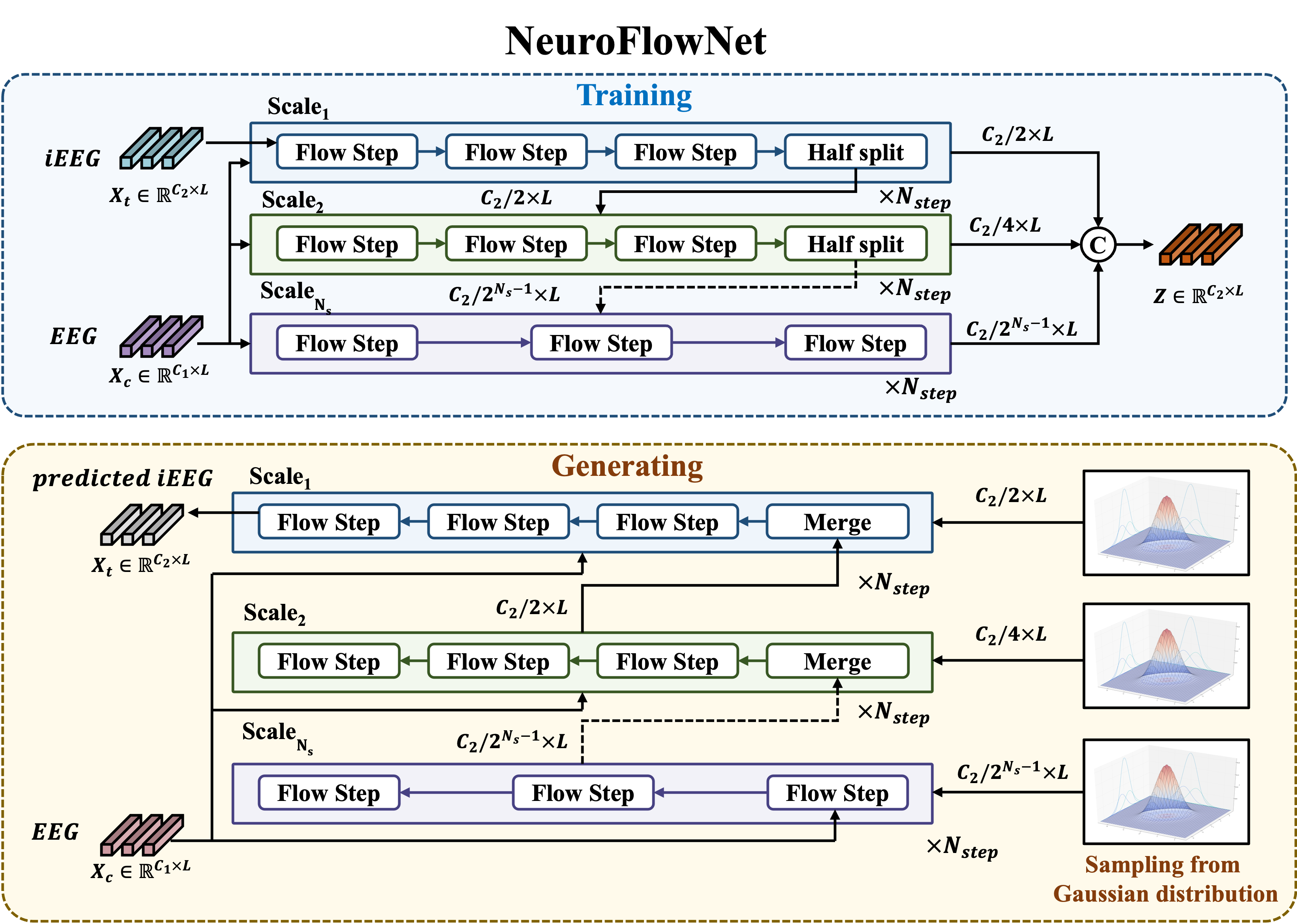
The proposed model, NeuroFlowNet, demonstrated in Figure 1, is designed to generate iEEG signals from non-invasive EEG signals by learning the cinditional probability distribution of iEEG given EEG, $p(X_{t}|X_{c})$, where $X_{t}\in\mathbb{R}^{C_{out}\times L}$ represents the target iEEG signals and $X_{c}\in\mathbb{R}^{C_{in}\times L}$ represents the conditioning EEG signals, with $C_{out}$ and $C_{in}$ being the number of channels of iEEG and EEG, respectively, and $L$ denoting the temporal length of the signals. NeuroFlowNet is architected as a multi-scale conditional normalizing flow, which transforms the complex distribution of iEEG data, conditioned on EEG data, into a simple, tractable base distribution (typically a standard multivariate Gaussian) via a sequence of invertible and differentiable transformations. The conditioning on EEG signals $X_{c}$ is achieved through a series of coupling layers, where the transformation is conditioned on the EEG data. The model is trained using a maximum likelihood estimation approach, optimizing the parameters of the transformations to maximize the likelihood of the observed iEEG data given the EEG data.

2.1 Core Invertible Transformation: Conditional Affine Coupling Layer

The core of the NeuroFlowNet architecture is the conditional affine coupling layer, which allows for the transformation of the iEEG data while conditioning on the EEG data. The coupling layer operates by splitting the input data into two parts: one part is transformed while the other part through an identity transformation. Specifically, given an input vector $x\in\mathbb{R}^{C\times L}$ at any stage of the flow, it is first split along the channel dimension into two halves, $x_{a}\in\mathbb{R}^{C/2\times L}$ and $x_{b}\in\mathbb{R}^{C/2\times L}$. The first half, $x_{a}$, is is passed through an identity transformation, while the second half, $x_{b}$, is transformed using a conditional affine transformation parameterized by a neural network. The transformation can be expressed as:

$$z_{b}=(x_{b}+\tau)\odot\text{exp}(\sigma)$$ (1)

where $\odot$ denotes element-wise multiplication. The translation parameters $\tau\in\mathbb{R}^{C/2\times L}$ and the log-scale parameters $\sigma\in\mathbb{R}^{C/2\times L}$ are produced by a conditional neural network, denoted as $g_{cond}$, which takes $x_{a}$ and the conditioning EEG data $X_{c}$ as inputs, and outputs the parameters $\tau$ and $\sigma$:

$$\begin{bmatrix}\tau\\ \sigma\end{bmatrix}=g_{cond}(x_{a},X_{c})$$ (2)

The conditional neural network $g_{cond}$ is designed to capture the complex relationships between the iEEG and EEG data, allowing for a more accurate transformation of the iEEG data based on the conditioning EEG data. The $g_{cond}$ network is composed of an initial couple of convolutional layers with kernel size of 3 and 1, respectively, both followed by a ReLU activation function. Specifically, the first convolutional layers with kernel size of 3 captures local temporal features from the input data and projects the input to a higher-dimensional feature space $\mathbb{R}^{C_{h}\times L}$, and the second convolutional layer with kernel size of 1 serves as a channel-wise linear transformation, further processing the features while maintaining the temporal resolution. The output of the second convolutional layer is then fed into a multi-head self-attention mechanism to capture long-range dependencies in the data, which is crucial for modeling the complex temporal dynamics of iEEG signals.

The multi-head self-attention mechanism allows the model to capture multiple relationships between the input data and the conditioning data by using multiple sets of query, key, and value matrices, each with different learned parameters. The output of the attention mechanism is then passed through a final convolutional layer with kernel size of 3 to produce the final parameters $\tau$ and $\sigma$. For numerical stability, translation parameters $\tau$ is scaled by a hyperbolic tangent function (tanh) to ensure that the values are bounded between -1 and 1, while the log-scale parameters $\sigma$ are clipped to a range of [-5, 5] to prevent numerical instability during the training process. The log-determinant of the Jacobian for this affine transformation is given by the sum of the log-scale factors:

$$\log\left|\det\frac{\partial z_{b}}{\partial x_{b}}\right|=\sum_{i,j}\sigma_{i,j}$$ (3)

The output of the coupling layer is $z=\text{concatenate}(x_{a},z_{b})$. The inverse transformation is obtained by applying the inverse of the affine transformation, which can be expressed as:

$$x_{b}=\text{exp}(-\sigma)\odot(z_{b}-\tau)$$ (4)

where the inverse transformation is applied to the transformed data $z_{b}$ to recover the original data $x_{b}$.

The inverse transformation is also computed in a similar manner, where the translation and log-scale parameters are obtained from the same conditional neural network $g_{cond}$, but with the input data being the transformed data $z_{a}$ and the conditioning EEG data $X_{c}$, i.e.:

$$\begin{bmatrix}\tau\\ \sigma\end{bmatrix}=g_{cond}(z_{a},X_{c})$$ (5)

2.2 Flow Step Composition

Figure 2: Flow step composition in NeuroFlowNet. Each flow step consists of an invertible $1\times 1$ convolution followed by a conditional affine coupling layer, which transforms the input data while conditioning on the EEG data $X_{c}$.

As demonstrated in Figure 2, each flow step within NeuroFlowNet combines the conditional affine coupling layer with an invertible channel-mixing operation to enhance the expressive power of the model. Specifically, before the input $x$ is fed into the affine coupling layer, it undergoes an invertible $1\times 1$ convolutional operation, a channel-wise linear transformation, $y=Wx^{\prime}$, where $x^{\prime}$ is the input to the flow step and $W\in\mathbb{R}^{C\times C}$ is a learnable weight matrix, which is initialized as an orthonormal matrix (via QR decomposition of a random Gaussian matrix) to ensure invertibility from the start of training and promote stability. This $1\times 1$ convolution allows for information to be mixed across channels at each temporal location independently. The log-determinant of the Jacobian for this transformation is:

$$\log\left|\det\frac{\partial y}{\partial x^{\prime}}\right|=L\cdot\log|\det W|$$ (6)

The total log-determinant for a single flow step is the sum of the log-determinants from the $1\times 1$ convolution and the subsequent conditional affine coupling layer. The inverse of the flow step involves applying the inverse affine coupling transformation followed by multiplication with $W^{-1}$.

2.3 Multi-Scale Architecture

The proposed NeuroFlowNet employs a multi-scale architecture to effectively model features and dependencies at varying resolutions within the iEEG signals. The model comprises $N_{S}$ hierarchical scales. At each scale $k\in\{1,\ldots,N_{S}\}$, the input, target iEEG signal $X_{t}$ at the first scale or the output from the preceding finer scale $(k-1)$, is processed through a sequence of $N_{\text{steps}}$ identical flow steps, as detailed in Section 2.2, with all transformations are conditioned on the EEG signal $X_{c}$.

Following the flow steps at scale $k$, the resulting tensor $y^{(k)}\in\mathbb{R}^{C_{k}\times L}$ is split along the channel dimension. A subset of channels, $z_{\text{part}}^{(k)}\in\mathbb{R}^{C_{k}/2\times L}$, is extracted and designated as part of the final latent variable $Z$. The remaining channels, $x_{\text{in}}^{(k+1)}\in\mathbb{R}^{C_{k}/2\times L}$, are propagated as input to the subsequent, typically coarser, scale $(k+1)$. The number of channels $C_{k}$ is halved at each successive scale, facilitating a progressive abstraction of features.

This hierarchical processing strategy enables the model to decompose the learning task, capturing fine-grained details at the initial scales and progressively more abstract, global representations at deeper levels. The final output from the coarsest scale, $z_{\text{final}}^{(N_{S})}\in\mathbb{R}^{C_{N_{S}}\times L}$, also contributes to the complete latent representation. The full latent variable $Z$ is obtained by concatenating all extracted components and the final output:

$$Z=\text{concatenate}(z_{\text{part}}^{(1)},z_{\text{part}}^{(2)},\ldots,z_{\text{part}}^{(N_{S}-1)},z_{\text{final}}^{(N_{S})})\in\mathbb{R}^{C_{out}\times L}$$ (7)

where $C_{out}=\sum_{k=1}^{N_{S}}C_{k}/2+C_{N_{S}}$ is the total number of channels in the latent variable $Z$

2.4 Training and Inference

2.4.1 Training

NeuroFlowNet is trained by maximizing the exact log-likelihood of the iEEG data $X_{t}$ given the EEG context $X_{c}$. Algorithm 1 outlines the training procedure. Let $f$ denote the overall transformation from the data space to the latent space, such that $Z=f(X_{t},X_{c})$. The log-likelihood of the iEEG data can be expressed as:

$$\log p(X_{t}\mid X_{c})=\log p_{Z}(Z)+\sum_{i=1}^{M}\log\left|\det\frac{\partial z_{i}}{\partial z_{i-1}}\right|$$ (8)

where $M$ is the total number of elementary invertible transformations that map the input $X_{t}$ to the final latent variable $Z$ (as defined in Equation 7), $z_{0}=X_{t}$ and $z_{i}$ is the output of the $i$-th transformation acting on its input $z_{i-1}$, then the final result of these $M$ transformations is $Z$. The term $\frac{\partial z_{i}}{\partial z_{i-1}}$ is the Jacobian matrix of this $i$-th transformation. $p_{Z}(Z)$ is the log-probability density of $Z$ under a standard multivariate Gaussian distribution $\mathcal{N}(0,I)$, which serves as the base distribution. The sum term $\sum_{i=1}^{M}\log\left|\det\frac{\partial z_{i}}{\partial z_{i-1}}\right|$ is the accumulated sum of the log-determinants of these Jacobians for all constituent invertible transformations ($1\times 1$ convolutions and affine coupling layers) across all flow steps and scales.

The model parameters are optimized by maximizing this log-likelihood objective:

$$\theta^{*}=\arg\max_{\theta}\log p(X_{t}\mid X_{c};\theta)$$ (9)

where $\theta$ represents the parameters of the model, including the weights of the conditional neural network $g_{cond}$ and the weights of the $1\times 1$ convolutions.

Algorithm 1 Training Phase of NeuroFlowNet (Forward & Parameter Update)

1:Batch $\{X_{c},X_{t}\}$, model parameters $\theta$, per-scale splits $\{S_{k}\}_{k=1}^{N_{S}}$, time length $L$

2:Updated parameters $\theta$ by maximizing $\log p(X_{t}\mid X_{c})$

3:Initialize $\log\_det\_total\leftarrow\mathbf{0}_{B}$, $o\leftarrow X_{t}$, $\mathcal{Z}\leftarrow\varnothing$

4:for $k=1\to N_{S}$ do

5:  $\log\_det_{k}\leftarrow\mathbf{0}_{B}$

6:  for $i=1\to N_{\text{steps}}$ do $\triangleright$ FlowStep $i$ in scale $k$

7:   $u\leftarrow\text{1x1conv}_{W^{(k)}_{i}}(o)$

8:   $\Delta_{\mathrm{conv}}\leftarrow L\cdot\operatorname{slogdet}\bigl(W^{(k)}_{i}\bigr)$ $\triangleright$ scalar

9:   $[u_{a},u_{b}]\leftarrow\text{split\_half}(u)$

10:   $[\tau,\sigma]\leftarrow g_{\text{cond}}(u_{a},X_{c};\theta_{\text{aff}})$

11:   $\tau\leftarrow 10\cdot\tanh(\tau),\ \sigma\leftarrow\operatorname{clamp}(\sigma,-5,5)$

12:   $z_{b}\leftarrow(u_{b}+\tau)\odot\exp(\sigma)$

13:   $o\leftarrow\operatorname{concat}(u_{a},z_{b})$

14:   $\Delta_{\mathrm{affine}}\leftarrow\sum_{c,t}\sigma_{c,t}$ $\triangleright$ per-sample vector of size $B$

15:   $\log\_det_{k}\leftarrow\log\_det_{k}+(\Delta_{\mathrm{conv}}+\Delta_{\mathrm{affine}})$

16:  end for

17:  $z^{(k)}\leftarrow o[:,\,1:S_{k},\,:]$ $\triangleright$ extract latent part

18:  $o\leftarrow o[:,\,S_{k}+1:C_{k},\,:]$ $\triangleright$ remaining channels to next scale

19:  append $z^{(k)}$ to $\mathcal{Z}$

20:  $\log\_det\_total\leftarrow\log\_det\_total+\log\_det_{k}$

21:end for

22:append final $o$ to $\mathcal{Z}$ $\triangleright$ final leftover latent

23:$Z\leftarrow\operatorname{concat}(\mathcal{Z},\ \text{channel})$

24:$\log p_{Z}\leftarrow-\tfrac{1}{2}\sum_{c,t}\bigl(Z^{2}+\log(2\pi)\bigr)$ $\triangleright$ per-sample

25:$\mathcal{L}\leftarrow-\frac{1}{B}\sum_{b=1}^{B}\bigl(\log p_{Z}^{(b)}+\log\_det\_total^{(b)}\bigr)$

26:Backpropagate $\mathcal{L}$ and update $\theta$ (e.g., AdamW step)

2.4.2 Inference (iEEG Generation)

To generate iEEG samples $\hat{X}_{t}$ conditioned on a given EEG signal $X_{c}$, the inverse transformation $f^{-1}$ is employed. Algorithm 2 outlines the inference procedure. First, a sample $\hat{Z}$ is drawn from the base Gaussian distribution $p_{Z}(Z)$. This $\hat{Z}$ is then partitioned into segments $\hat{z}^{(1)}_{part},\ldots,\hat{z}^{(N_{S}-1)}_{part},\hat{z}^{(N_{S})}_{final}$ corresponding to the multi-scale splitting performed during the forward pass. The generation process starts from the coarsest scale $N_{S}$. The segment $\hat{z}^{(N_{S})}_{final}$ is transformed by applying the inverse of the flow steps within the $N_{S}$-th scale block. For each subsequent finer scale $k$ (iterating from $N_{S}-1$ down to $1$), the corresponding latent segment $\hat{z}^{(k)}_{part}$ is concatenated with the output from the inverse transformation of the preceding coarser scale $(k+1)$. This combined tensor is then passed through the inverse flow steps of scale $k$. All inverse transformations are conditioned on the EEG context $X_{c}$. The final output of this sequential inverse process, after passing through the inverse of the first scale block, is the generated iEEG sample $\hat{X}_{t}=f^{-1}(\hat{Z};X_{c})$.

Algorithm 2 Inference / Sampling Phase of NeuroFlowNet (Inverse Mapping)

1:Conditioning $X_{c}$, model parameters $\theta$, per-scale splits $\{S_{k}\}_{k=1}^{N_{S}}$, optional $\varepsilon\in\mathbb{R}^{B\times D\times L}$

2:Generated iEEG samples $\hat{X}_{t}$

3:if no $\varepsilon$ provided then

4:  sample $\varepsilon\sim\mathcal{N}(0,I)$ $\triangleright$ shape matches total latent channels

5:end if

6:split $\varepsilon$ into parts $\{\tilde{z}^{(1)},\dots,\tilde{z}^{(N_{S})},\tilde{z}^{(N_{S}+1)}\}$ according to $\{S_{k},\ldots\}$

7:$o\leftarrow\tilde{z}^{(N_{S}+1)}$ $\triangleright$ start from coarsest latent

8:for $k=N_{S}\to 1$ do $\triangleright$ reverse through scales

9:  $o\leftarrow\operatorname{concat}(\tilde{z}^{(k)},\,o)$ $\triangleright$ reconstruct full channel tensor at scale $k$

10:  for each FlowStep $i=N_{\text{steps}},\dots,1$ (reversed order) do

11:   $[z_{a},z_{b}]\leftarrow\text{split\_half}(o)$

12:   $[\tau,\sigma]\leftarrow g_{\text{cond}}(z_{a},X_{c};\theta_{\text{aff}})$

13:   $\tau\leftarrow 10\cdot\tanh(\tau),\ \sigma\leftarrow\operatorname{clamp}(\sigma,-5,5)$

14:   $u_{b}\leftarrow\exp(-\sigma)\odot(z_{b}-\tau)$ $\triangleright$ affine inverse

15:   $u\leftarrow\operatorname{concat}(z_{a},u_{b})$

16:   $o\leftarrow\text{1x1conv}_{W^{-1}}(u)$ $\triangleright$ apply inverse 1x1 conv

17:  end for

18:end for

19:Output: $\hat{X}_{t}\leftarrow o$

3 Experiments

3.1 Dataset

Figure 3: Medial temporal lobe (MTL) depth electrode locations for subjects used in this study (S1, S6 and S9). Each panel shows coronal, sagittal, and axial views of depth electrode trajectories within MTL subregions. Colors indicate anatomical targets: anterior hippocampus (AHL/AHR, red/light red), amygdala (AL/AR, orange/yellow), entorhinal cortex (ECL/ECR, green/light green), parahippocampal gyrus (PHL/PHR, purple/magenta), and lateral rhinal area (LR, blue). Each trajectory consists of eight electrode contacts positioned along a single stereotactic path.

This study utilizes an electrophysiological dataset recorded from nine epilepsy patients during a verbal working memory task, as introduced by Boran et al. [9], which is publicly available at https://gin.g-node.org/USZ_NCH/Human_MTL_units_scalp_EEG_and_iEEG_verbal_WM. The dataset includes simultaneous EEG recorded using the 10-20 system and iEEG obtained via depth microelectrodes implanted in the medial temporal lobe (MTL). The EEG and iEEG signals are originally sampled at 256 Hz and 4 kHz, respectively, and later resampled to 200 Hz and 2 kHz. It also contains waveforms and spike times of 1526 single units, along with MNI coordinates in MNI152 space and anatomical labels for the intracranial electrodes.

The nine subjects (five female, four male) are all right-handed and aged between 18 and 56. Their pathologies include hippocampal sclerosis, gliosis, xanthoastrocytoma, brain contusion, and focal cortical dysplasia. Each participant has a varying number and location of implanted depth electrodes within the MTL. Due to significant inter-subject variability in electrode implantation (both in terms of anatomical coverage and number of recorded units), only subjects S1, S6, and S9 were included in this study. These three subjects were selected because (i) they have comprehensive electrode coverage across key MTL subregions of interest, (ii) they exhibit a sufficient number of well-isolated single units for reliable statistical analysis, and (iii) their recording sessions contained minimal artifacts and consistent task performance. Due to clinical considerations and individualized implantation plans, the exact anatomical locations of intracranial electrodes differ across subjects [9]. To illustrate this variability, Figure 3 presents a 3D schematic of depth electrode trajectories in the MTL for three subjects (S1, S6 and S9) used in this study.

Each subject completes between two and seven recording sessions. Table 1 summarizes the characteristics of the subjects, including their personal information, pathologies, implanted scalp and intracranial electrodes, and number of sessions. The EEG signals are recorded using the international 10-20 system, with electrodes placed at standard locations such as Fp1, Fp2, F7, F3, Cz, Pz, O1, and O2. The iEEG signals are recorded from depth microelectrodes targeting multiple MTL subregions: anterior hippocampus (AHL/AHR), amygdala (AL/AR), entorhinal cortex (ECL/ECR), and parahippocampal gyrus (PHL/PHR), as well as lateral rhinal area (LR). Each trajectory consisted of eight microelectrode contacts arranged along a single stereotactic path.

The dataset provides a rich source of electrophysiological data, allowing for the exploration of cross-modal generation of iEEG signals from EEG signals. The iEEG signals are used as the target signals $X_{t}$ for model training and evaluation, while the EEG signals are used as the conditioning input $X_{c}$. The dataset is suitable for training and evaluating the NeuroFlowNet model, as it contains a diverse set of subjects with varying pathologies and electrode placements. The model aims to learn the complex relationships between the non-invasive EEG signals and the invasive iEEG signals, enabling the generation of iEEG signals from EEG data.

Table 1: Subject Characteristics

No.	Age	Sex	Pathology	Implanted electrodes	Sessions
1	24	F	Xanthoastrocytoma WHO II	F3, F4, C3, C4, P3, P4, O1, O2, F7, F8, T3, T4, T5, T6, Fz, Cz, Pz, A1, A2	4
				AHL, AL, ECL, LR, PHL, PHR
2	39	M	Gliosis	F3, F4, C3, C4, O1, O2, A1, A2	7
				AHL, AHR, AL, AR, ECL, ECR, PHL, PHR
3	18	F	Hippocampal sclerosis	F3, F4, C3, C4, O1, O2, A1, A2	3
				AHL, AHR, AL, ECL, PHL
4	28	M	Brain contusion	F3, F4, C3, C4, P3, P4, O1, O2, F7, F8, T3, T4, T5, T6, Fz, Cz, Pz, A1, A2	2
				AHL, AHR, AL, AR, ECL, ECR, PHL, PHR
5	20	F	Focal cortical dysplasia	Fp1, Fp2, F3, F4, C3, C4, P3, P4, O1, O2, F7, F8, T4, T5, T6, Fz, Cz, Pz, A1, A2	3
				AHL, AL, DRR, PHR
6	31	M	Hippocampal sclerosis	Fp1, Fp2, F3, F4, C3, C4, O1, O2, A1, A2	7
				AHL, AHR, AL, AR, ECL, ECR, PHL, PHR
7	47	M	Hippocampal sclerosis	F3, F4, C3, C4, O1, O2, A1, A2	4
				AHL, AHR, AL, AR, ECL, ECR, PHL, PHR
8	56	F	Hippocampal sclerosis	F3, F4, C3, C4, P3, P4, O1, O2, F7, F8, T3, T4, T5, T6, Fz, Cz, Pz, A1, A2	5
				AHL, AHR, AL, AR, ECL, ECR, PHL, PHR
9	19	F	Hippocampal sclerosis	F3, F4, C3, C4, O1, O2, A1, A2	2
				AHL, AHR, AL, AR, ECL, ECR, PHL, PHR

¹ Each iEEG electrode label corresponds to eight depth microelectrode contacts positioned along a single trajectory.
² Abbreviations for MTL Regions: AHL/AHR - Anterior Hippocampus (Left/Right), AL/AR - Amygdala (Left/Right), ECL/ECR - Entorhinal Cortex (Left/Right), PHL/PHR - Parahippocampal Gyrus (Left/Right), LR - Lateral Rhinal Area, DRR - Dorsal Rhinal Region.

3.2 Data Preprocessing and Division

The iEEG and EEG signals are preprocessed to remove artifacts and noise, ensuring high-quality data for model training. The preprocessing steps include wavelet denoising, downsampling, data division, and normalization.

The wavelet denoising is performed using the discrete wavelet transform (DWT) with Symlet wavelets of order 4 (sym4), which helps suppress broadband noise while retaining the main morphological characteristics of the signals. A three-level decomposition is applied to each channel independently, producing the coefficient set ${A_{3},D_{3},D_{2},D_{1}}$, where $A_{3}$ denotes the level-3 approximation coefficients and $D_{\ell}$ denotes the detail coefficients at level $\ell$. The approximation coefficients $A_{3}$ are retained without modification, and soft-thresholding is applied to all detail sub-bands ${D_{1},D_{2},D_{3}}$. The noise level is estimated using the median absolute deviation (MAD) computed over the concatenation of detail coefficients across levels, $\hat{\sigma}=\mathrm{median}(|\mathrm{concat}(D_{1},D_{2},D_{3})|)/0.6745$. A universal threshold is then determined based on the segment length (n) (number of time samples) as $T=\hat{\sigma}\sqrt{2\ln(n)}$, and each detail coefficient (w) is shrunk via soft thresholding $\mathcal{S}_{T}(w)=\mathrm{sign}(w)\max(|w|-T,0)$. Finally, the denoised signal is reconstructed by inverse DWT (IDWT) with symmetric boundary extension, and the reconstructed sequence is cropped to the original length to ensure temporal alignment with the original signal.

In this work, to align the temporal grid between modalities for supervised cross-modal learning, we further downsampled iEEG to 200 Hz using an explicit anti-aliasing procedure, which constrains the analyzable bandwidth to $\leq$100 Hz (and our evaluations to 0.5-50 Hz / 8-13 Hz). Specifically, to prevent aliasing, we apply an explicit anti-aliasing low-pass filter prior to decimation: iEEG is first low-pass filtered with a cutoff below the target Nyquist frequency (100 Hz) and a transition band (implemented in a zero-phase manner via forward-backward filtering), and then resampled to 200 Hz using a polyphase/decimation routine. As a consequence, the maximum representable frequency after downsampling is 100 Hz, and all frequency-domain evaluations and claims in this paper are restricted to the preserved low-/mid-frequency range (PSD: 0.5-50 Hz; alpha: 8-13 Hz; see Table 2).

Each subject participates in multiple recording sessions, and each session consists of multiple trials of the verbal working memory task. Due to the individualized clinical implantation schemes (i.e., subject-specific electrode locations, trajectories, and the number of available contacts/units), the intracranial targets and coverage are not directly comparable across subjects; therefore, a controlled cross-subject generalization setting is not feasible with this dataset. Accordingly, we adopt a subject-specific (within-subject) evaluation protocol, where models are trained and validated using data from the same subject. Within each session, we first perform a trial-level split by randomly assigning 90% of trials to the training set and the remaining 10% to the validation set. This trial-level split ensures that the model is evaluated on unseen trials, providing a more robust assessment of its generalization capabilities within the same subject. The training and validation trials are further divided into smaller segments of 200 samples (1 second) used a sliding window approach with a 90% overlap for training sets, while the validation set is divided into segments of 200 samples with no overlap. The Z-score normalization is applied to each segment, ensuring that the mean and standard deviation of the signals are zero and one, respectively. This normalization step is crucial for stabilizing the training process and improving the model’s performance.

3.3 Hyperparameter Selection and Ablation Study

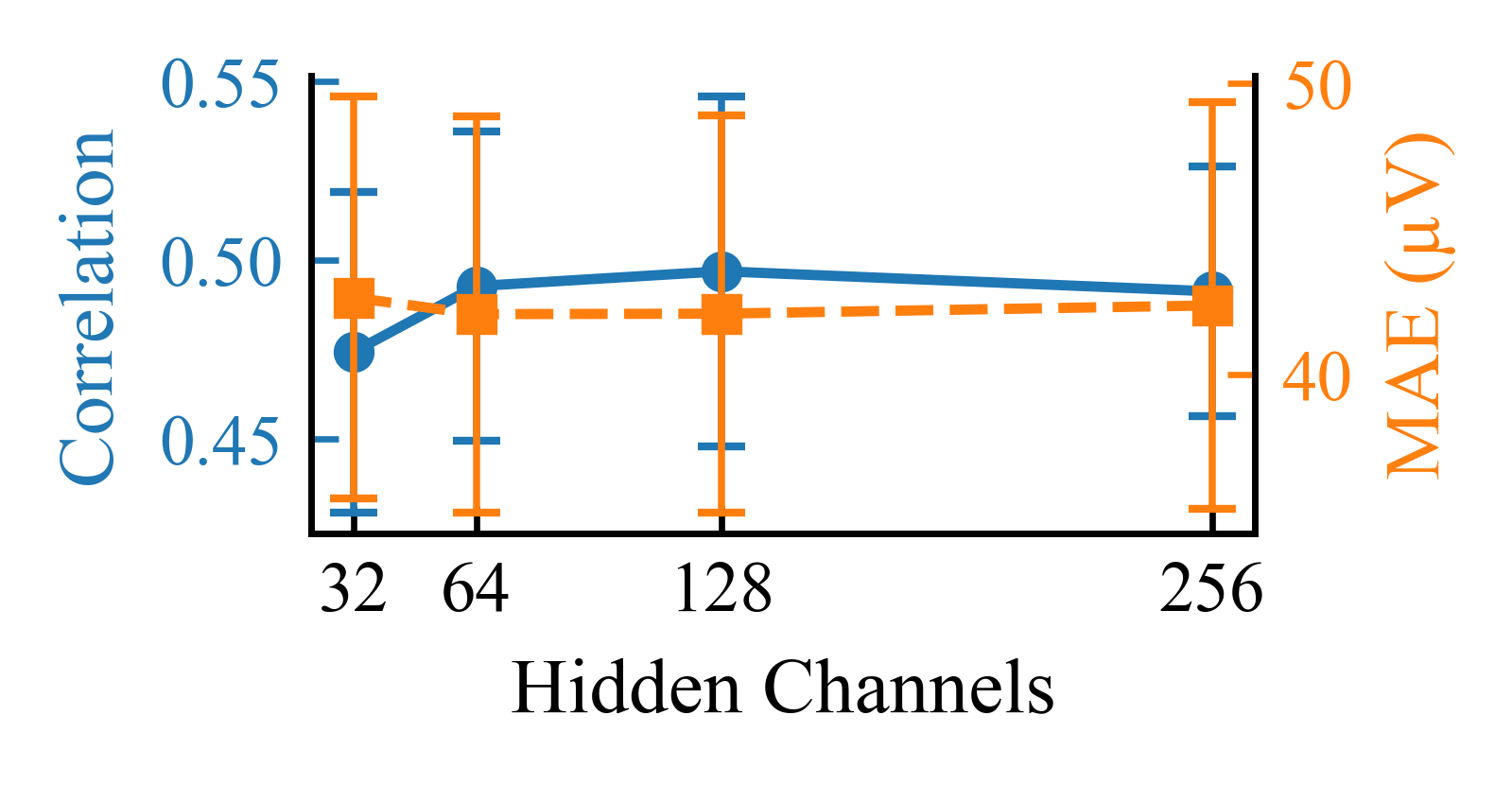
The performance of the NeuroFlowNet model is influenced by several key hyperparameters, including the number of scales $N_{S}$, the number of flow steps per scale $N_{\text{steps}}$, and the number of channels in the hidden layers of the conditional neural network $C_{h}$. To determine the optimal values for these hyperparameters, we conducted a systematic evaluation using a one-factor-at-a-time (OFAT) approach. This method involves varying one hyperparameter while keeping the others fixed at their default values, allowing us to isolate the effect of each hyperparameter on model performance. The candidate values for each hyperparameter were selected based on preliminary experiments and domain knowledge. The performance of the model was evaluated on the validation set and averaged across all subjects to ensure that the selected hyperparameters generalize well across different individuals. Specifically, as shown in Figure 4(a), varying the number of scales $N_{S}\in\{1,2,3\}$ leads to a small improvement when increasing from $N_{S}=1$ to $N_{S}=2$ (higher correlation with lower MAE). Further increasing to $N_{S}=3$ brings no consistent gain, with performance remaining essentially unchanged within the error bars. As illustrated in Figure 4(b), we evaluated the number of flow steps per scale $N_{\text{steps}}\in\{2,4,6,8\}$. The correlation improves as $N_{\text{steps}}$ increases up to 6, while MAE shows only minor variation; increasing to $N_{\text{steps}}=8$ yields no clear additional benefit. Finally, as shown in Figure 4(c), we assessed the effect of the hidden channels $C_{h}\in\{32,64,128,256\}$ in the conditional network. The model achieves the best (or near-best) validation performance at $C_{h}=128$, whereas smaller widths underperform slightly and a larger width ($C_{h}=256$) does not improve results. Based on these observations and considering computational efficiency, we select $N_{S}=2$, $N_{\text{steps}}=6$, and $C_{h}=128$ as the hyperparameter setting for training NeuroFlowNet.

(a) $N_{S}$ (number of scales)

(b) $N_{\text{steps}}$ (flow steps per scale)

(c) $C_{h}$ (hidden channels)

Figure 4: Hyperparameter selection results for NeuroFlowNet. The performance of the model is evaluated on the validation set and averaged across all subjects and electrodes. The hyperparameters include $N_{S}$, the number of scales (a); $N_{\text{steps}}$, the number of flow steps per scale (b); and $C_{h}$, the number of channels in the hidden layers of the conditional neural network (c). The results indicate that the model achieves optimal performance with $N_{S}=2$, $N_{\text{steps}}=6$, and $C_{h}=128$.

To validate the architectural choice of the conditional network $g_{cond}$ in the affine coupling layers, we conduct a controlled ablation by removing the MHSA module from $g_{cond}$ while keeping all other components and training/evaluation settings unchanged. Figure 5 summarizes the results on the validation set. Overall, incorporating MHSA yields better performance when averaged across subjects and electrodes. The mean correlation increases from $0.479\pm 0.077$ (No MHSA) to $0.497\pm 0.060$ (With MHSA), and the mean MAE decreases from $42.74\pm 9.66~\mu$V to $42.09\pm 8.35~\mu$V (mean$\pm$std across subjects and electrodes). These results suggest that MHSA strengthens $g_{cond}$ in capturing cross-modal dependencies between EEG and iEEG, improving reconstruction consistency (higher correlation) and slightly reducing amplitude error (lower MAE) on average. This ablation provides component-level evidence that the attention mechanism is a beneficial design element in $g_{cond}$ for cross-modal generation.

Figure 5: Ablation of the MHSA module in the conditional network $g_{cond}$. Correlation (higher is better) and MAE (lower is better) are reported on the validation set. Bars indicate the mean across subjects and electrodes, and error bars denote the standard deviation across subjects

3.4 Implementation Details

The NeuroFlowNet model is implemented using PyTorch, a popular deep learning framework. The model architecture consists of multiple scales, each containing a series of flow steps that transform the iEEG data conditioned on the EEG data. The model is trained using the AdamW optimizer with a learning rate of $1\times 10^{-3}$ and a weight decay of $1\times 10^{-2}$. The model is trained on a single NVIDIA RTX 4080 GPU with 16 GB of memory. The batch size is set to 128, and the model is trained for 100 epochs. The $N_{S}$ (number of scales), $N_{\text{steps}}$ (number of flow steps per scale) and $C_{h}$ (number of channels in the hidden layers of the conditional neural network) are treated as hyperparameters. Candidate values are chosen empirically and then evaluated on the validation set using OFAT procedure, where one hyperparameter is varied while the others are fixed, as illustrated in Section 3.3. The final model architecture is set to have $N_{S}=2$ scales, with $N_{\text{steps}}=6$ flow steps per scale, and $C_{h}=128$ channels in the hidden layers of the conditional neural network. The model is trained separately for each subject, and the best-performing model on the validation set is selected. Early stopping is implemented based on the performance on the validation set, with a patience of 10 epochs.

4 Results and Discussion

Table 2: Performance of NeuroFlowNet on iEEG signal generation.

Subject	Region	Temporal waveform			PSD waveform (0.5-50Hz)		Alpha PSD waveform (8-13Hz)
		MAE (µV)	Corr	Cosine	Corr	Cosine	Corr	Cosine	Power MAPE (%)
S1	AHL	40.66 $\pm$ 21.53	0.35 $\pm$ 0.28	0.47 $\pm$ 0.24	0.66 $\pm$ 0.22	0.70 $\pm$ 0.19	0.25 $\pm$ 0.53	0.70 $\pm$ 0.21	2.65 $\pm$ 4.40
	AL	42.82 $\pm$ 28.98	0.39 $\pm$ 0.30	0.50 $\pm$ 0.26	0.67 $\pm$ 0.23	0.71 $\pm$ 0.20	0.29 $\pm$ 0.52	0.71 $\pm$ 0.21	3.33 $\pm$ 7.35
	ECL	49.15 $\pm$ 27.35	0.40 $\pm$ 0.25	0.50 $\pm$ 0.21	0.66 $\pm$ 0.24	0.70 $\pm$ 0.21	0.32 $\pm$ 0.52	0.72 $\pm$ 0.21	6.49 $\pm$ 16.65
	LR	33.86 $\pm$ 20.08	0.60 $\pm$ 0.28	0.65 $\pm$ 0.25	0.76 $\pm$ 0.23	0.79 $\pm$ 0.20	0.45 $\pm$ 0.48	0.78 $\pm$ 0.18	1.24 $\pm$ 2.18
	PHL	35.68 $\pm$ 15.08	0.56 $\pm$ 0.33	0.62 $\pm$ 0.28	0.74 $\pm$ 0.23	0.77 $\pm$ 0.20	0.44 $\pm$ 0.49	0.77 $\pm$ 0.20	1.23 $\pm$ 2.87
	PHR	82.42 $\pm$ 72.44	0.24 $\pm$ 0.29	0.39 $\pm$ 0.27	0.53 $\pm$ 0.25	0.59 $\pm$ 0.22	0.23 $\pm$ 0.53	0.70 $\pm$ 0.20	2.85 $\pm$ 5.36
S6	AHL	44.08 $\pm$ 27.47	0.44 $\pm$ 0.23	0.51 $\pm$ 0.21	0.61 $\pm$ 0.21	0.67 $\pm$ 0.18	0.33 $\pm$ 0.51	0.74 $\pm$ 0.19	1.58 $\pm$ 3.63
	AHR	40.80 $\pm$ 21.73	0.58 $\pm$ 0.21	0.63 $\pm$ 0.19	0.68 $\pm$ 0.20	0.73 $\pm$ 0.17	0.48 $\pm$ 0.50	0.80 $\pm$ 0.19	0.95 $\pm$ 1.88
	AL	45.78 $\pm$ 19.99	0.46 $\pm$ 0.23	0.52 $\pm$ 0.21	0.63 $\pm$ 0.21	0.67 $\pm$ 0.18	0.39 $\pm$ 0.48	0.76 $\pm$ 0.19	1.75 $\pm$ 2.97
	AR	26.77 $\pm$ 9.21	0.74 $\pm$ 0.16	0.77 $\pm$ 0.14	0.78 $\pm$ 0.17	0.81 $\pm$ 0.15	0.67 $\pm$ 0.38	0.87 $\pm$ 0.14	0.61 $\pm$ 1.01
	ECL	53.71 $\pm$ 21.22	0.49 $\pm$ 0.23	0.54 $\pm$ 0.21	0.67 $\pm$ 0.21	0.71 $\pm$ 0.18	0.37 $\pm$ 0.51	0.75 $\pm$ 0.19	1.75 $\pm$ 3.41
	ECR	34.92 $\pm$ 14.32	0.64 $\pm$ 0.17	0.68 $\pm$ 0.16	0.71 $\pm$ 0.20	0.75 $\pm$ 0.18	0.59 $\pm$ 0.43	0.84 $\pm$ 0.15	1.05 $\pm$ 2.48
	PHL	25.73 $\pm$ 15.79	0.39 $\pm$ 0.29	0.49 $\pm$ 0.25	0.60 $\pm$ 0.21	0.66 $\pm$ 0.18	0.32 $\pm$ 0.51	0.74 $\pm$ 0.20	1.38 $\pm$ 2.51
	PHR	36.89 $\pm$ 16.07	0.60 $\pm$ 0.20	0.64 $\pm$ 0.18	0.70 $\pm$ 0.19	0.74 $\pm$ 0.17	0.51 $\pm$ 0.45	0.79 $\pm$ 0.18	0.84 $\pm$ 1.53
S9	AHL	29.92 $\pm$ 10.79	0.67 $\pm$ 0.19	0.73 $\pm$ 0.15	0.81 $\pm$ 0.17	0.82 $\pm$ 0.16	0.36 $\pm$ 0.49	0.73 $\pm$ 0.20	0.88 $\pm$ 1.24
	AHR	43.49 $\pm$ 26.44	0.38 $\pm$ 0.28	0.50 $\pm$ 0.24	0.69 $\pm$ 0.23	0.71 $\pm$ 0.21	0.20 $\pm$ 0.55	0.67 $\pm$ 0.22	7.20 $\pm$ 14.62
	AL	35.30 $\pm$ 11.46	0.61 $\pm$ 0.19	0.66 $\pm$ 0.16	0.78 $\pm$ 0.19	0.80 $\pm$ 0.17	0.34 $\pm$ 0.50	0.72 $\pm$ 0.21	1.45 $\pm$ 3.01
	AR	29.48 $\pm$ 21.12	0.34 $\pm$ 0.34	0.46 $\pm$ 0.30	0.64 $\pm$ 0.25	0.68 $\pm$ 0.22	0.22 $\pm$ 0.54	0.67 $\pm$ 0.23	4.82 $\pm$ 8.81
	ECL	38.73 $\pm$ 17.66	0.55 $\pm$ 0.25	0.61 $\pm$ 0.21	0.75 $\pm$ 0.22	0.77 $\pm$ 0.20	0.34 $\pm$ 0.52	0.72 $\pm$ 0.22	1.62 $\pm$ 2.73
	ECR	43.11 $\pm$ 18.69	0.44 $\pm$ 0.26	0.51 $\pm$ 0.23	0.71 $\pm$ 0.22	0.74 $\pm$ 0.20	0.24 $\pm$ 0.52	0.70 $\pm$ 0.21	3.46 $\pm$ 5.78
	PHL	26.60 $\pm$ 14.10	0.73 $\pm$ 0.20	0.78 $\pm$ 0.17	0.84 $\pm$ 0.16	0.85 $\pm$ 0.15	0.46 $\pm$ 0.46	0.77 $\pm$ 0.18	0.93 $\pm$ 1.39
	PHR	38.48 $\pm$ 17.46	0.49 $\pm$ 0.26	0.55 $\pm$ 0.25	0.74 $\pm$ 0.22	0.76 $\pm$ 0.20	0.33 $\pm$ 0.51	0.71 $\pm$ 0.21	5.35 $\pm$ 10.49

¹ The results of each region are averaged across all electrodes within that region.
² Abbreviations for MTL Regions: AHL/AHR - Anterior Hippocampus (Left/Right), AL/AR - Amygdala (Left/Right), ECL/ECR - Entorhinal Cortex (Left/Right), PHL/PHR - Parahippocampal Gyrus (Left/Right), LR - Lateral Rhinal Area.

The performance of NeuroFlowNet is evaluated based on its ability to generate iEEG signals from EEG signals in terms of temporal waveform, power spectral density (PSD) waveform, alpha PSD waveform and functional connection mode. The results reveal a clear pattern of region- and subject-specific variability, reflecting both the strengths and current limitations of the model.

4.1 Temporal Waveform Comparison

Figure 6: Exemplar generated iEEG signals (orange) overlaid with ground truth iEEG signals (blue) for various MTL subregions, specifically showing a 200ms segment from Subject S6. The figure illustrates the performance of NeuroFlowNet in generating iEEG signals from EEG data across different anatomical targets, including anterior hippocampus (AHL/AHR), amygdala (AL/AR), entorhinal cortex (ECL/ECR), and parahippocampal gyrus (PHL/PHR).

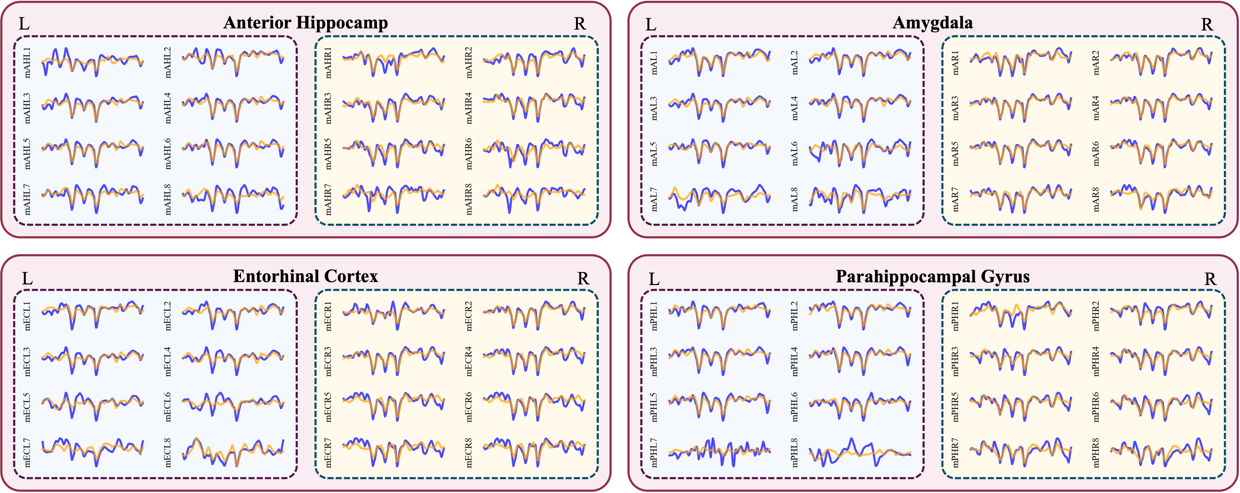
A qualitative assessment of the model’s performance is presented in Figure 6, which displays exemplar generated iEEG signals (orange) overlaid with the corresponding ground truth iEEG signals (blue) for a 200ms segment from Subject S6. The figure provides a visual comparison across various MTL subregions, including the anterior hippocampus (AHL/AHR), amygdala (AL/AR), entorhinal cortex (ECL/ECR), and parahippocampal gyrus (PHL/PHR). As showed in Figure 6, the generated waveforms demonstrate a high degree of fidelity to the ground truth signals, successfully capturing the principal morphological characteristics and temporal dynamics. The model effectively replicates both the slower, underlying oscillations and the relatively faster fluctuations that remain observable under the 200 Hz bandwidth. The alignment is particularly strong in regions such as the amygdala and the parahippocampal gyrus, where the generated signals closely trace the contours of the ground truth waveforms in terms of phase and relative amplitude.

In more structurally complex or deeper regions, such as the anterior hippocampus and entorhinal cortex, the model still captures the general trend of the signal but occasionally shows minor discrepancies in peak amplitude or precise temporal alignment. For instance, some of the fast transients in the ground truth signal are slightly smoothed or have a marginally lower amplitude in the generated counterpart. Nevertheless, the overall correspondence remains robust, underscoring NeuroFlowNet’s capability to learn the complex conditional mapping from non-invasive EEG to invasive iEEG signals across multiple anatomical targets. This visual evidence corroborates that the model generates temporally coherent and physiologically plausible iEEG waveforms.

To quantify the temporal waveform performance metrics of the model (mean absolute error (MAE), Pearson correlation coefficient (Corr), and cosine similarity), Table 2 summarizes the results for multiple MTL subregions across three subjects (S1, S6, S9). The results demonstrate that NeuroFlowNet exhibits varying efficacy in restoring the temporal dynamics of iEEG signals from different MTL subregions

Specifically, consistent with anatomical proximity to the scalp, more superficial or lateral regions such as the amygdala (AL/AR) and parahippocampal gyrus (PHL/PHR) generally show higher correlations and cosine similarities. For example, in subject S9, the parahippocampal gyrus (PHL) achieves a correlation coefficient of 0.73 $\pm$ 0.20 and a cosine similarity of 0.78 $\pm$ 0.17, indicating strong alignment in waveform shape and direction . In contrast, deeper structures like the anterior hippocampus (AHL/AHR) present greater challenges: subject S1’s AHL region shows notably lower performance (Corr: 0.35 $\pm$ 0.28, Cosine: 0.47 $\pm$ 0.24), reflecting difficulties in capturing the complex signal dynamics of deep brain areas.

Notably, MAE values often diverge from correlation metrics. For instance, in subject S6’s entorhinal cortex (ECL), a moderate correlation (0.49 $\pm$ 0.23) coexists with a relatively high MAE (53.71 $\pm$ 21.22 µV), suggesting potential discrepancies in amplitude scaling . Such inconsistencies may stem from the model’s sensitivity to inter-individual variations in signal amplitude and anatomical differences in electrode implantation locations.

4.2 Power Spectral Density Comparison

To evaluate the frequency reproduction capability within the preserved bandwidth of NeuroFlowNet, Figure 7 shows a comparison of the PSD waveforms of the generated signals (orange) and the actual signals (blue) for eight MTL subregions of subject S6. The PSD waveform for each region is the average of all electrodes in that region. The analysis reveals that NeuroFlowNet successfully captures the salient spectral characteristics of the native iEEG signals. Across all depicted regions, the generated PSDs closely mirror the ground truth within the preserved bandwidth, particularly in replicating the prominent power peak in the alpha band (8-13 Hz) and a secondary peak in the theta band (4-8 Hz) [28, 32]. These frequency bands are physiologically critical in the MTL; theta oscillations are integral to memory encoding and retrieval, while alpha rhythms are associated with functional inhibition and attentional modulation. The model’s accurate generation of these peaks indicates that it learns to infer the state of these underlying cognitive processes from the conditioning EEG data. Furthermore, the model correctly reproduces the aperiodic, 1/f-like decay in power at higher frequencies, a hallmark of background neural activity [23, 37]. This demonstrates a robust generalization beyond just the dominant oscillatory components.

To further scrutinize the model’s performance on the functionally significant alpha band, Figure 8 provides a detailed analysis of generated versus true alpha power. The scatter plot (Figure 8a) shows a strong positive correlation, with the linear fit line (y=0.67x+0.13) closely following the ideal line (y=x). This indicates that the model reliably captures the relative changes in alpha power. The slope of less than one suggests a slight regression to the mean, where the model may temper the most extreme high or low power values, a common characteristic when inferring high-resolution signals from lower signal-to-noise data. The Bland-Altman plot (Figure 8b) reinforces this finding by showing that the mean difference between true and generated alpha power is exceptionally low (0.01), indicating no systematic bias in the model’s predictions. The data points are evenly scattered within the 95% limits of agreement, confirming that while individual predictions have some variance, the model’s estimations are, on average, highly accurate. Collectively, the spectral analysis demonstrates that NeuroFlowNet generates iEEG signals that are not only temporally plausible but also spectrally realistic, preserving the key neurophysiological frequency fingerprints essential for downstream analysis.

Figure 7: Comparison of power spectral density (PSD) between ground truth iEEG signals (blue) and generated iEEG signals (orange) for a 200 ms segment from Subject S6. The figure shows the average PSD across all electrodes within each MTL subregion, including anterior hippocampus (AHL/AHR), amygdala (AL/AR), entorhinal cortex (ECL/ECR), and parahippocampal gyrus (PHL/PHR).

Figure 8: (a) Scatter plot of normalized true alpha power versus normalized generated alpha power. The red dashed line represents the ideal line (y = x), while the green solid line indicates the linear fit (y = 0.67x + 0.13). (b) Bland-Altman plot showing the difference in alpha power against the mean alpha power. The red dashed line indicates the mean difference (0.01), and the green and blue dashed lines represent the upper (95% CI, 0.28) and lower (95% CI, -0.27) limits of agreement, respectively.

To quantify the frequency domain reproduction capability of the model, Table 2 summarizes the results for multiple MTL subregions of three subjects (S1, S6, and S9), 0.5-50 Hz PSD waveform metrics (Corr and cosine similarity), and 8-13 Hz $\alpha$ PSD waveform metrics (Corr, cosine similarity, and mean absolute percentage error (MAPE)). In the broad frequency range (0.5-50 Hz), NeuroFlowNet demonstrates relatively stable performance across MTL regions. PSD correlation coefficients range from 0.53 $\pm$ 0.25 (PHR, S1) to 0.84 $\pm$ 0.16 (PHL, S9), indicating reliable preservation of spectral composition despite temporal waveform variability . While most regions exhibit PSD cosine similarities exceeding 0.70, an exception is observed in S1’s PHR region (0.59 $\pm$ 0.22), highlighting minor regional variability. For the alpha band (8-13 Hz), cosine similarities remain stable (0.70-0.87), but correlations fluctuate significantly, such as 0.22 $\pm$ 0.54 in S9’s AR region versus 0.67 $\pm$ 0.38 in S6’s AR region . Alpha power MAPE is generally low (below 3% for most regions), but outliers include S1’s ECL (6.49 $\pm$ 16.65%), S9’s AHR (7.20 $\pm$ 14.62%), and S9’s PHR (5.35 $\pm$ 10.49%) . This suggests the model struggles with precise alpha-phase capture but effectively estimates relative power distributions, critical for neurophysiological applications focusing on oscillatory activity [5, 58, 66].

4.3 Inter-Channel Correlation Comparison

Figure 9: Comparison of inter-channel correlation. Circular graphs show the connectivity patterns of (a) the original iEEG signals and (b) the generated iEEG signals. Both plots illustrate a 200 ms segment from Subject S6. Pairwise Pearson correlation coefficients are computed between all channels, and only the top 50 strongest absolute correlations are visualized for clarity.

Beyond generating realistic single-channel waveforms, a crucial test for the model is its ability to capture the complex functional relationships between different neural populations. These relationships are reflected in the inter-channel correlation structure of the iEEG signals. Figure 9 presents a qualitative comparison of these correlation patterns, displaying the 50 strongest pairwise Pearson correlations for both the ground truth (a) and generated (b) iEEG signals from a 200ms segment of Subject S6.

The circular plots reveal a remarkable correspondence between the ground truth and the generated data. The model successfully reproduces the salient features of the functional connectivity network. Key patterns, such as strong correlations between homologous regions in the left and right hemispheres (e.g., between channels in AHL and AHR), are clearly preserved. This is physiologically significant as it reflects the synchronous activity maintained between bilateral structures via commissural pathways.

Furthermore, the model accurately captures strong correlations between anatomically and functionally connected regions within the same hemisphere, such as the connections between the entorhinal cortex and the hippocampus, which form a critical circuit for memory processing. The visual similarity of the two plots—from the dense connections within the parahippocampal gyrus to the sparser but strong links spanning distant regions—indicates that NeuroFlowNet is not merely generating a collection of independent, albeit realistic, time series. Instead, it is learning the underlying covariance structure that governs the system-level dynamics of the Medial Temporal Lobe network. This ability to replicate the spatial organization of neural activity is a strong indicator that the generated iEEG data retains the neurophysiological signatures necessary for more advanced network-level analyses.

4.4 Functional Connectivity Fidelity Comparison with Regression Baselines and Discussion

Table 3: Functional connectivity fidelity (inter-channel correlation structure) comparison between NeuroFlowNet and regression baselines.

Matrix	Linear (1$\times$1)	Shallow CNN	1D U-Net	Tiny Transformer	NeuroFlowNet (Ours)
$\mathcal{E}_{\mathrm{MAE}}(\mathbf{R})$	0.426 $\pm$ 0.064	0.318 $\pm$ 0.032	0.302 $\pm$ 0.013	0.360 $\pm$ 0.080	0.288 $\pm$ 0.042
$\mathcal{E}_{F}(\mathbf{R})$	30.45 $\pm$ 6.45	23.37 $\pm$ 3.99	22.08 $\pm$ 2.57	26.04 $\pm$ 6.86	21.61 $\pm$ 4.69

Note: $\mathbf{R}$ denotes the inter-channel Pearson correlation matrix computed over time for each 1-second segment. $\mathcal{E}_{\mathrm{MAE}}(\mathbf{R})=\frac{1}{C^{2}}\lVert\mathbf{R}^{\text{pred}}-\mathbf{R}^{\text{true}}\rVert_{1}$ and $\mathcal{E}_{F}(\mathbf{R})=\lVert\mathbf{R}^{\text{pred}}-\mathbf{R}^{\text{true}}\rVert_{F}$, averaged within each subject and then across subjects, reported as mean $\pm$ std.

As emphasized above, an important requirement for non-invasive iEEG reconstruction is not only waveform plausibility at each channel, but also the preservation of inter-channel correlation structure that reflects MTL functional connectivity. In practice, many downstream analyses in cognitive and clinical neuroscience rely on network-level signatures (e.g., co-fluctuations across contacts/regions), and a model that produces visually plausible traces yet distorts cross-channel dependencies may be of limited utility for connectivity-driven interpretation. Therefore, we complement our within-model connectivity demonstration with a controlled comparison to representative deterministic regression baselines under the same subject-specific protocol described in Section 4.3.

We compare NeuroFlowNet with four aligned sequence-to-sequence regression baselines: (i) a pointwise linear mapping implemented as a $1\times 1$ convolution (Linear), (ii) a shallow 1D CNN regressor (Shallow CNN), (iii) a non-causal 1D U-Net regressor (1D U-Net), and (iv) a tiny Transformer regressor (Tiny Transformer). All models are trained and evaluated using the same subject-specific setting (S1, S6, S9), the same trial-level split (90%/10%), and the same segmentation strategy (1-second windows of 200 samples; training windows with overlap and validation windows without overlap), following Section 3.2. This ensures that any performance differences are attributable to modeling choices rather than data partitioning or preprocessing.

For each 1-second segment, we compute the Pearson inter-channel correlation matrix $\mathbf{R}\in\mathbb{R}^{C\times C}$ from the iEEG channels over the time axis. Let $\mathbf{R}^{\text{pred}}$ and $\mathbf{R}^{\text{true}}$ denote the predicted and ground-truth correlation matrices, respectively. We report two matrix-level errors:

$$\mathcal{E}_{\mathrm{MAE}}(\mathbf{R})=\frac{1}{C^{2}}\left\lVert\mathbf{R}^{\text{pred}}-\mathbf{R}^{\text{true}}\right\rVert_{1},\quad\mathcal{E}_{F}(\mathbf{R})=\left\lVert\mathbf{R}^{\text{pred}}-\mathbf{R}^{\text{true}}\right\rVert_{F},$$ (10)

where $\lVert\cdot\rVert_{1}$ is the element-wise $\ell_{1}$ norm and $\lVert\cdot\rVert_{F}$ is the Frobenius norm. Metrics are first averaged within each subject and then across subjects (S1, S6, S9), reported as mean$\pm$std. Lower values indicate better preservation of multi-channel functional connectivity structure.

Table 3 summarizes the functional connectivity fidelity across models. NeuroFlowNet achieves the lowest errors among the compared methods, with $\mathcal{E}_{\mathrm{MAE}}(\mathbf{R})=0.288\pm 0.042$ and $\mathcal{E}_{F}(\mathbf{R})=21.61\pm 4.69$. Compared with the pointwise linear baseline, NeuroFlowNet reduces correlation-matrix MAE from $0.426\pm 0.064$ to $0.288\pm 0.042$ (a relative reduction of $\sim$32%), and reduces Frobenius error from $30.45\pm 6.45$ to $21.61\pm 4.69$ (a relative reduction of $\sim$29%). This indicates that a simple per-time linear mapping is insufficient to recover the network-level dependencies embedded in MTL iEEG activity, whereas NeuroFlowNet better captures higher-order cross-channel structure under the same training data regime.

Beyond the linear baseline, NeuroFlowNet also consistently outperforms the stronger nonlinear regressors included in this comparison (Shallow CNN, 1D U-Net, and Tiny Transformer). While these deterministic models can learn nonlinear mappings and often generate temporally smooth outputs, they still tend to emphasize pointwise signal reconstruction objectives, which can inadvertently attenuate or homogenize cross-channel relationships—especially when the inverse mapping from scalp EEG to deep iEEG is underconstrained. In such ill-posed settings, a deterministic regressor is incentivized to output a “central” solution that reduces average prediction error across trials, which may appear reasonable at the level of individual traces but can shrink trial-to-trial covariance and distort the correlation matrix. The observed gap in $\mathcal{E}_{\mathrm{MAE}}(\mathbf{R})$ and $\mathcal{E}_{F}(\mathbf{R})$ suggests that NeuroFlowNet better preserves the correlation structure that is most relevant for functional connectivity analyses, aligning with the qualitative similarity of connectivity graphs shown in Figure 9.

A plausible explanation for this advantage lies in the inductive biases of conditional normalizing flows and the specific architectural design of NeuroFlowNet. First, CNF optimizes exact conditional likelihood, enabling the model to represent the conditional distribution of iEEG given EEG rather than collapsing all variability into a single deterministic output. Conceptually, this is consistent with the non-uniqueness of EEG inverse problems: multiple intracranial configurations can give rise to similar scalp observations due to volume conduction and source mixing. By introducing a latent variable and learning an invertible mapping, NeuroFlowNet can retain residual degrees of freedom that are not fully determined by EEG, instead of forcing them into a mean prediction. This helps preserve realistic trial-level co-variations across channels, which directly manifest as more faithful correlation matrices.

The invertible $1\times 1$ convolution in each flow step provides an explicit channel-mixing mechanism. Unlike standard convolutions that may learn channel interactions implicitly (and potentially inconsistently across layers), the invertible mixing operation encourages structured information exchange across channels at every temporal location while maintaining reversibility. This is particularly relevant in multi-channel iEEG, where functional connectivity is encoded in coordinated activity patterns across contacts/regions. By repeatedly mixing channels through invertible transforms, the model can more effectively capture and propagate global cross-channel dependencies throughout the flow, which can improve the fidelity of reconstructed correlation structure.

In addition, the multi-scale architecture further supports structure preservation by decomposing the learning problem across resolutions. Fine scales focus on local temporal detail, whereas coarser scales capture more global, slowly varying patterns that often drive connectivity estimates. Since correlation matrices integrate information over time, errors in low-frequency or large-scale components can disproportionately affect connectivity fidelity. The hierarchical split-and-propagate design allows NeuroFlowNet to allocate capacity to both local waveform characteristics and global coordination patterns, which may explain its stronger performance in $\mathcal{E}_{\mathrm{MAE}}(\mathbf{R})$ and $\mathcal{E}_{F}(\mathbf{R})$.

These findings should be interpreted within the subject-specific scope of this dataset. The present comparison demonstrates that, under identical within-subject training conditions, NeuroFlowNet yields improved functional connectivity fidelity relative to representative deterministic regressors. This supports our central claim that modeling the conditional distribution with an invertible multi-scale architecture is beneficial for preserving the inter-channel correlation structure of MTL iEEG. Future work will extend these connectivity-driven evaluations to broader cohorts and more diverse brain states, and will assess whether connectivity preservation translates into improved performance on downstream tasks that explicitly rely on network-level features (e.g., connectivity-based decoding or seizure network characterization).

4.5 Discussion of Physiological Determinants in Regional Variability

The observed performance heterogeneity across MTL subregions can be partially attributed to neuroanatomical and physiological factors. In terms of structural complexity, the anterior hippocampus (AHL/AHR) is characterized by intricate laminar organization and high neuronal density, resulting in complex and non-linear iEEG signal patterns [39]. This complexity likely exceeds the current representational capacity of NeuroFlowNet’s conditional normalizing flow, contributing to reduced fidelity in this region [63]. Besides, deeply situated structures like AHL experience greater signal attenuation in EEG recordings due to intervening tissues (cerebrospinal fluid, skull), reducing the signal-to-noise ratio of the conditioning data and complicating accurate inference of iEEG dynamics [29]. In contrast, more superficial regions such as the parahippocampal gyrus benefit from proximity to the cortical surface, aiding model performance [60]. Additionally, regions with strong cortico-MTL connectivity, such as the entorhinal cortex (ECL/ECR), may exhibit iEEG dynamics that are more inferable from scalp-recorded potentials, aligning with their relatively high temporal and spectral performance [64].

4.6 Discussion of Bandwidth Limitation

A key preprocessing step in this work is downsampling iEEG from 2 kHz to 200 Hz to match scalp EEG and to enforce an aligned temporal grid for conditional modeling. While this alignment is important for stable supervised training and fair cross-modal comparison, it imposes an explicit bandwidth constraint: after downsampling, the effective Nyquist frequency is 100 Hz, and spectral content above 100 Hz cannot be represented. In addition, the required anti-aliasing low-pass filter (applied before decimation/resampling) can attenuate components near the cutoff, which may further reduce the sharpness of rapid fluctuations even below 100 Hz. This limitation is particularly relevant for intracranial biomarkers that are typically studied in higher frequency ranges, such as high-gamma activity and high-frequency oscillations, as well as very fast transient events. These phenomena are not the target of the present reconstruction setting and cannot be faithfully assessed under a 200 Hz sampling pipeline. Accordingly, the term “high-fidelity” in this study refers to the fidelity within the preserved bandwidth of the preprocessing chain, rather than broadband fidelity across the full spectrum available in the original 2 kHz iEEG.

Consistent with this scope, our quantitative frequency-domain evaluations are restricted to low-/mid-frequency bands, specifically PSD similarity in 0.5-50 Hz and alpha-band (8-13 Hz) characteristics (Table 2). Moreover, our functional-connectivity analyses rely on inter-channel correlation matrices computed from these band-limited time series, and our conclusions are therefore confined to (i) temporal waveform plausibility at 200 Hz resolution, (ii) preservation of low-/mid-frequency spectral fingerprints, and (iii) recovery of inter-channel dependency structure within this bandwidth.

Future work will extend the framework toward higher-frequency intracranial signatures by (i) training and evaluating at higher target sampling rates (e.g., 500 Hz or 1 kHz) when synchronized EEG-iEEG data of sufficient quality are available, and/or (ii) adopting multi-resolution modeling strategies in which low-frequency components are reconstructed at 200 Hz for cross-modal alignment while higher-frequency components are modeled with an additional dedicated branch or a hierarchical refinement stage. These directions would enable a more comprehensive assessment of whether non-invasive EEG can support reconstruction of clinically and cognitively relevant high-frequency iEEG biomarkers beyond the present band-limited setting.

4.7 Discussion of Physiological Interpretation of the Latent Space Representation $Z$

To further strengthen the interpretability of NeuroFlowNet, we discuss the potential physiological meaning of the learned latent representation $Z$. In conditional normalizing flows, $Z$ is obtained through an invertible transformation $Z=f(X_{t},X_{c})$, where $X_{t}$ and $X_{c}$ denote the target iEEG and conditioning scalp EEG, respectively. Due to the bijective nature of the flow mapping, $Z$ should not be interpreted as a single physiological “source” or a direct anatomical generator in the classical sense. Instead, we view $Z$ as a compact parametrization of the residual degrees of freedom in intracranial activity that are not uniquely constrained by scalp EEG, i.e., a principled representation of the conditional uncertainty in $p(X_{iEEG}\mid X_{EEG})$ [46].

From a neurophysiological perspective, this residual component can plausibly reflect multiple factors. First, it may capture trial-to-trial variability of local circuit dynamics within the MTL that is only weakly expressed on the scalp due to volume conduction, source mixing, and limited signal-to-noise ratio [4, 67, 50]. Second, it may encode micro-scale and transient activity (e.g., sharp fluctuations and other local population events) that substantially shapes iEEG waveforms but is attenuated or spatially smeared in scalp recordings [50, 3, 41]. Third, it may represent state-dependent stochastic modulations of ongoing rhythms, where fluctuations in cognitive state or vigilance alter intracranial oscillatory patterns without being fully predictable from scalp EEG alone [49]. Importantly, this interpretation is consistent with the well-known non-uniqueness of EEG inverse problems: multiple intracranial configurations can produce similar scalp observations, and introducing a latent variable provides a natural probabilistic mechanism to represent this ambiguity rather than forcing a single deterministic reconstruction [4, 67].

This perspective also helps contextualize the regional variability discussed above. For deeper or more structurally complex targets (e.g., the anterior hippocampus), scalp observability is expected to be reduced, and thus a larger portion of iEEG variability may remain underconstrained by EEG [50, 3, 61]. In NeuroFlowNet, such underconstrained components are naturally represented through the latent pathway $Z$, enabling the model to avoid collapsing to an “average” waveform and instead generate diverse yet EEG-consistent iEEG samples [46]. We emphasize that the above points constitute a physiologically motivated interpretation of $Z$ rather than a definitive identification of specific neural generators. Future work will validate these hypotheses using dedicated interpretability analyses (e.g., linking latent factors to band-limited power modulation, event-related signatures, or unit/spike-informed markers) on larger cohorts with broader brain-state coverage [10].

4.8 Discussion of Clinical Translation and Robustness Considerations

Although NeuroFlowNet demonstrates the feasibility of reconstructing MTL iEEG patterns from scalp EEG on a public synchronized EEG-iEEG dataset, the current evidence should be interpreted within a subject-specific and task-dependent scope [10]. In this dataset, recordings were obtained from epilepsy patients with individualized implantation schemes, and intracranial electrode coverage is not standardized across subjects [34]. As a result, direct cross-subject generalization cannot be rigorously established with the present data. Therefore, while our findings support the methodological potential of non-invasive iEEG reconstruction, they do not yet justify strong clinical claims, particularly for high-stakes applications such as non-invasive pre-surgical localization [34].

Clinical translation of EEG-to-iEEG reconstruction ultimately depends on robust performance across both subjects and brain states. Inter-subject variability arises from differences in anatomy, skull conductivity, pathology, medication, and electrode implantation targets, all of which can alter the scalp-to-intracranial mapping [61, 4, 67]. Cross-state variability is also expected, as intracranial dynamics change substantially across vigilance and cognitive conditions (e.g., rest vs. task engagement), and across clinically relevant contexts (e.g., interictal vs. ictal periods) [49, 34]. These factors may introduce distribution shifts that challenge purely subject-specific modeling and motivate broader validation [50, 3].

To move toward clinical readiness, several steps are necessary. First, larger multi-subject datasets with more comparable intracranial coverage (or standardized ROI definitions) are required to enable systematic evaluation of cross-subject generalization and the development of adaptation strategies that account for anatomical and physiological differences [34, 61]. Second, robustness should be assessed across heterogeneous brain states, ideally including resting state, sleep, multiple cognitive tasks, and interictal/ictal segments, to establish state generalization [49, 34]. Third, the clinical value of reconstructed signals should be validated in downstream endpoints where performance can be directly linked to decision-making, such as interictal spike detection, seizure onset zone (SOZ) localization, or surgical outcome prediction [34]. Taken together, we position NeuroFlowNet as a methodological step toward non-invasive deep-brain signal inference, while recognizing that comprehensive cross-subject and cross-state validation is an essential prerequisite for clinical translation [34].

5 Conclusion

In this study, we introduced NeuroFlowNet, a novel generative framework based on conditional normalizing flows, to address the enduring challenge of generating high-fidelity (band-limited) iEEG from non-invasive EEG within the preserved bandwidth. Our work makes a pivotal contribution by demonstrating, for the first time, the feasibility of reconstructing iEEG signals across multiple MTL subregions. By directly modeling the conditional probability distribution, NeuroFlowNet fundamentally overcomes the mode collapse and deterministic mapping limitations of previous generative models. Our results confirm that the generated signals not only achieve high fidelity in temporal waveforms and spectral characteristics but also successfully preserve the complex inter-channel correlation structure, reflecting the underlying functional connectivity of the MTL network. In addition, a baseline comparison against representative deterministic regressors shows that NeuroFlowNet yields lower errors in the inter-channel correlation matrix under the same within-subject protocol, supporting its advantage in structure-preserving reconstruction rather than purely pointwise fitting. The ability to generate realistic, probabilistic iEEG provides a powerful new tool for both clinical and research applications, offering a non-invasive window into deep brain dynamics. This could significantly improve our understanding of cognitive processes governed by the MTL, potentially reducing the reliance on high-risk invasive procedures.

However, we acknowledge certain limitations. The model’s performance exhibits variability across different MTL subregions, with deeper and more structurally complex areas like the anterior hippocampus proving more challenging to reconstruct accurately. This suggests that the signal-to-noise ratio of the conditioning EEG and the inherent complexity of the target signal are key performance determinants. Additionally, since iEEG is downsampled to 200 Hz with anti-aliasing, the present results and spectral claims are limited to the preserved low-/mid-frequency range ($\leq$100 Hz; evaluated mainly in 0.5-50 Hz and 8-13 Hz), and do not address high-frequency intracranial biomarkers such as high-gamma/HFO. Moreover, the present study does not yet establish cross-subject or cross-state generalization, and clinical deployment should be considered premature until validated on larger cohorts and heterogeneous brain states.

Future work will focus on three main directions: 1) Enhancing the model architecture by incorporating more sophisticated conditioning mechanisms that can better leverage spatial information from the EEG montage. 2) Expanding the framework to a subject-independent model by collecting larger-scale datasets with more standardized and comparable electrode implantation coverage across subjects, which will enable a systematic evaluation of cross-subject generalization and support the development of advanced domain adaptation techniques to account for inter-subject anatomical and physiological variability. 3) Validating the clinical utility of the generated iEEG in downstream tasks, such as automated seizure detection and cognitive state decoding, to bridge the gap between technical innovation and practical application.

CRediT authorship contribution statement

Dongyi He: Conceptualization, Methodology, Software, Data curation, Writing - original draft, Writing - review & editing, Visualization. Bin Jiang: Conceptualization, Supervision, Writing - review & editing, Funding acquisition, Writing - original draft, Formal analysis. Kecheng Feng: Writing - review & editing, Visualization, Formal analysis. Luyin Zhang: Writing - review & editing. Ling Liu: Writing - review & editing. Yuxuan Li: Writing - review & editing. Yun Zhao: Funding acquisition, Formal analysis, Writing - review & editing, Supervision, Resources He Yan: Supervision, Resources All authors have read and approved the final manuscript.

Declaration of competing interest

The authors declare that they have no known competing financial interests or personal relationships that could have appeared to influence the work reported in this paper.

Ethics statement

This study was conducted in publicly available datasets, thus ethical approval was not required.

Declaration of generative AI and AI-assisted technologies in the writing process.

During the preparation of this work the author(s) used ChatGPT in order to check the grammar and spelling of the manuscript. After using this tool/service, the author(s) reviewed and edited the content as needed and take(s) full responsibility for the content of the published article.

Funding Declaration

This research was funded by the Scientific and Technological Research Program of the Chongqing Education Commission (KJZD-K202303103, KJQN202501104) and Chongqing Municipal Key Project for Technology Innovation and Application Development (CSTB2024TIAD-KPX0042).

References

- [1] (2023) Mapping scalp to intracranial eeg using generative adversarial networks for automatically detecting interictal epileptiform discharges. In 2023 IEEE Statistical Signal Processing Workshop (SSP), pp. 710–714. Cited by: §1.
- [2] (2025) EEG-to-eeg: scalp-to-intracranial eeg translation using a combination of variational autoencoder and generative adversarial networks. Sensors 25 (2), pp. 494. Cited by: §1.
- [3] (2024) EEG/meg source imaging of deep brain activity within the maximum entropy on the mean framework: simulations and validation in epilepsy. Human Brain Mapping 45 (10), pp. e26720. Cited by: §4.7, §4.7, §4.8.
- [4] (2020) A systematic review of eeg source localization techniques and their applications on diagnosis of brain abnormalities. Journal of neuroscience methods 339, pp. 108740. Cited by: §4.7, §4.8.
- [5] (2017) Oscillatory activities in neurological disorders of elderly: biomarkers to target for neuromodulation. Frontiers in Aging Neuroscience 9, pp. 189. Cited by: §4.2.
- [6] (2017) Magnetoencephalography for brain electrophysiology and imaging. Nature neuroscience 20 (3), pp. 327–339. Cited by: §1.
- [7] (2024) Inverse problem for m/eeg source localization: a review. IEEE Sensors Journal. Cited by: §1.
- [8] (2018) Brain-actuated functional electrical stimulation elicits lasting arm motor recovery after stroke. Nature communications 9 (1), pp. 2421. Cited by: §1.
- [9] (2019) Persistent hippocampal neural firing and hippocampal-cortical coupling predict verbal working memory load. Science advances 5 (3), pp. eaav3687. Cited by: §1, §3.1, §3.1.
- [10] (2020) Dataset of human medial temporal lobe neurons, scalp and intracranial eeg during a verbal working memory task. Scientific data 7 (1), pp. 30. Cited by: §4.7, §4.8.
- [11] (2021) A long short-term memory network for sparse spatiotemporal eeg source imaging. IEEE Transactions on Medical Imaging 40 (12), pp. 3787–3800. Cited by: §1.
- [12] (2018) Overview of deep learning architectures for eeg-based brain imaging. In 2018 International joint conference on neural networks (IJCNN), pp. 1–7. Cited by: §1.
- [13] (2023) Connectivity analysis in eeg data: a tutorial review of the state of the art and emerging trends. Bioengineering 10 (3), pp. 372. Cited by: §1.
- [14] (2024) HvEEGNet: a novel deep learning model for high-fidelity eeg reconstruction. Frontiers in Neuroinformatics 18, pp. 1459970. Cited by: §1.
- [15] (2019) Deep learning for electroencephalogram (eeg) classification tasks: a review. Journal of neural engineering 16 (3), pp. 031001. Cited by: §1.
- [16] (2019) EEG source localization using spatio-temporal neural network. China Communications 16 (7), pp. 131–143. Cited by: §1.
- [17] (2024) Scaling synthetic brain data generation. IEEE Journal of Biomedical and Health Informatics. Cited by: §1.
- [18] (2008) Review on solving the inverse problem in eeg source analysis. Journal of neuroengineering and rehabilitation 5 (1), pp. 25. Cited by: §1.
- [19] (2023) Review of eeg signals classification using machine learning and deep-learning techniques. In Advances in non-invasive biomedical signal sensing and processing with machine learning, pp. 159–183. Cited by: §1.
- [20] (2018) Electroencephalography source connectivity: aiming for high resolution of brain networks in time and space. IEEE Signal Processing Magazine 35 (3), pp. 81–96. Cited by: §1.
- [21] (2019) Electrophysiological brain connectivity: theory and implementation. IEEE transactions on biomedical engineering 66 (7), pp. 2115–2137. Cited by: §1.
- [22] (2018) Electrophysiological source imaging: a noninvasive window to brain dynamics. Annual review of biomedical engineering 20 (1), pp. 171–196. Cited by: §1.
- [23] (2014) Scale-free brain activity: past, present, and future. Trends in cognitive sciences 18 (9), pp. 480–487. Cited by: §4.2.
- [24] (2025) Spec2VolCAMU-net: a spectrogram-to-volume model for eeg-to-fmri reconstruction based on multi-directional time–frequency convolutional attention encoder and vision-mamba u-net. Journal of Neural Engineering 22 (5), pp. 056042. Cited by: §1.
- [25] (2021) ConvDip: a convolutional neural network for better eeg source imaging. Frontiers in Neuroscience 15, pp. 569918. Cited by: §1.
- [26] (2017) Comparison of the spatial resolution of source imaging techniques in high-density eeg and meg. Neuroimage 157, pp. 531–544. Cited by: §1.
- [27] (2020) The potential of stereotactic-eeg for brain-computer interfaces: current progress and future directions. Frontiers in neuroscience 14, pp. 123. Cited by: §1.
- [28] (2020) Theta oscillations in human memory. Trends in cognitive sciences 24 (3), pp. 208–227. Cited by: §4.2.
- [29] (2020) Localization of deep brain activity with scalp and subdural eeg. NeuroImage 223, pp. 117344. Cited by: §4.5.
- [30] (2022) Electromagnetic source imaging via a data-synthesis-based convolutional encoder–decoder network. IEEE Transactions on Neural Networks and Learning Systems 35 (5), pp. 6423–6437. Cited by: §1.
- [31] (2022) EEG dipole source localization using deep neural network. Int. J. Circuits Syst. Signal Process 16, pp. 132–140. Cited by: §1.
- [32] (2010) Shaping functional architecture by oscillatory alpha activity: gating by inhibition. Frontiers in human neuroscience 4, pp. 186. Cited by: §4.2.
- [33] (2026) A comprehensive review of deep learning for motor imagery eeg: from healthy subjects to patients. Biomedical Signal Processing and Control 117, pp. 109680. Cited by: §1.
- [34] (2020) Intracranial eeg in the 21st century. Epilepsy currents 20 (4), pp. 180–188. Cited by: §4.8, §4.8, §4.8.
- [35] (2024) Integrating electroencephalography source localization and residual convolutional neural network for advanced stroke rehabilitation. Bioengineering 11 (10), pp. 967. Cited by: §1.
- [36] (2013) Prior knowledge on cortex organization in the reconstruction of source current densities from eeg. Neuroimage 67, pp. 7–24. Cited by: §1.
- [37] (2023) The 1/f-like behavior of neural field spectra are a natural consequence of noise driven brain dynamics. bioRxiv. Cited by: §4.2.
- [38] (2022) A study on brain–computer interface: methods and applications. SN Computer Science 4 (2), pp. 98. Cited by: §1.
- [39] (2018) Optimal referencing for stereo-electroencephalographic (seeg) recordings. NeuroImage 183, pp. 327–335. Cited by: §4.5.
- [40] (2025) A tale of single-channel electroencephalogram: devices, datasets, signal processing, applications, and future directions. IEEE Transactions on Instrumentation and Measurement. Cited by: §1.
- [41] (2022) A consensus statement on detection of hippocampal sharp wave ripples and differentiation from other fast oscillations. Nature communications 13 (1), pp. 6000. Cited by: §4.7.
- [42] (2024) Attention-based convolutional neural network with multi-modal temporal information fusion for motor imagery eeg decoding. Computers in Biology and Medicine 175, pp. 108504. Cited by: §1.
- [43] (2019) EEG source imaging: a practical review of the analysis steps. Frontiers in neurology 10, pp. 325. Cited by: §1, §1, §1.
- [44] (2012) Human intracranial recordings and cognitive neuroscience. Annual review of psychology 63 (1), pp. 511–537. Cited by: §1.
- [45] (2019) EEG-based brain-computer interfaces using motor-imagery: techniques and challenges. Sensors 19 (6), pp. 1423. Cited by: §1.
- [46] (2021) Normalizing flows for probabilistic modeling and inference. Journal of Machine Learning Research 22 (57), pp. 1–64. Cited by: §4.7, §4.7.
- [47] (2018) Human intracranial eeg: promises and limitations. Nature neuroscience 21 (4), pp. 474. Cited by: §1.
- [48] (2018) Promises and limitations of human intracranial electroencephalography. Nature neuroscience 21 (4), pp. 474–483. Cited by: §1.
- [49] (2023) Vigilance described by the time-on-task effect in eeg activity during a cued go/nogo task. International Journal of Psychophysiology 183, pp. 92–102. Cited by: §4.7, §4.8, §4.8.
- [50] (2021) A comprehensive study on electroencephalography and magnetoencephalography sensitivity to cortical and subcortical sources. Human Brain Mapping 42 (4), pp. 978–992. Cited by: §4.7, §4.7, §4.8.
- [51] (2010) Neuroelectromagnetic source imaging of brain dynamics. In Computational Neuroscience, pp. 127–155. Cited by: §1.
- [52] (2025) Deep learning-based eeg source imaging is robust under varying electrode configurations. Clinical Neurophysiology. Cited by: §1.
- [53] (2025) SEEG in 2025: progress and pending challenges in stereotaxy methods, biomarkers and radiofrequency thermocoagulation. Current opinion in neurology 38 (2), pp. 111–120. Cited by: §1.
- [54] (2021) Neural decoding of eeg signals with machine learning: a systematic review. Brain sciences 11 (11), pp. 1525. Cited by: §1.
- [55] (2019) Subcortical electrophysiological activity is detectable with high-density eeg source imaging. Nature communications 10 (1), pp. 753. Cited by: §1.
- [56] (2020) Investigating the temporal dynamics of electroencephalogram (eeg) microstates using recurrent neural networks. Human brain mapping 41 (9), pp. 2334–2346. Cited by: §1.
- [57] (2015) Effect of eeg electrode number on epileptic source localization in pediatric patients. Clinical Neurophysiology 126 (3), pp. 472–480. Cited by: §1.
- [58] (2006) Neural synchrony in brain disorders: relevance for cognitive dysfunctions and pathophysiology. neuron 52 (1), pp. 155–168. Cited by: §4.2.
- [59] (2020) Multiple dipole source localization of eeg measurements using particle filter with partial stratified resampling. Biomedical engineering letters 10 (2), pp. 205–215. Cited by: §1.
- [60] (2020) Mapping the scene and object processing networks by intracranial eeg. Frontiers in human neuroscience 14, pp. 561399. Cited by: §4.5.
- [61] (2024) Global sensitivity of eeg source analysis to tissue conductivity uncertainties. Frontiers in Human Neuroscience 18, pp. 1335212. Cited by: §4.7, §4.8, §4.8.
- [62] (2025) A functional connectivity metric method for eeg time series via nonlinear symbolization. Biomedical Signal Processing and Control 103, pp. 107498. Cited by: §1.
- [63] (2019) Learning likelihoods with conditional normalizing flows. arXiv preprint arXiv:1912.00042. Cited by: §4.5.
- [64] (2025) Enhanced role of the entorhinal cortex in adapting to increased working memory load. Nature Communications 16 (1), pp. 5798. Cited by: §4.5.
- [65] (2025) RGFTSLANet: a cross-subject classification model for decoding eeg-based motor imagery tasks. In 2025 Cross Strait Radio Science and Wireless Technology Conference (CSRSWTC), pp. 1–4. Cited by: §1.
- [66] (2021) Relative power correlates with the decoding performance of motor imagery both across time and subjects. Frontiers in Human Neuroscience 15, pp. 701091. Cited by: §4.2.
- [67] (2021) Advances in electrical source imaging: a review of the current approaches, applications and challenges. Signals 2 (3), pp. 378–391. Cited by: §4.7, §4.8.