Political Shocks and Price Discovery in Prediction Markets: Evidence from the 2024 U.S. Presidential Election
Abstract
Using transaction-level trade data from Polymarket’s 2024 U.S. presidential election market, we study how prediction markets process shocks. We analyze three events: the Biden-Trump debate, the assassination attempt on Trump, and Biden’s dropout. Trading rises after each shock, especially among incumbent traders with pre-event exposure against a Trump victory, who are also more likely to flip positions. Price adjustment differs across shocks. The debate-induced price jump largely reverses, the assassination-attempt repricing persists, and Biden’s dropout triggers two-sided trading with little net price change. These patterns link post-news price dynamics to liquidity and disagreement about how shocks map into election odds.
Keywords: prediction markets; political shocks; price discovery; market microstructure; trader heterogeneity.
JEL Codes: G14; D84; D72.
1 Introduction
Prediction markets are often treated as real-time barometers of how breaking news changes beliefs about uncertain future events. Yet the first price move after a major shock is not informative on its own. The key questions are whether the market reacts quickly, which traders supply the marginal order flow, and whether the resulting price adjustment reflects durable updating in beliefs or temporary pressure in a thin market. This paper studies these questions jointly in the context of major political shocks in the 2024 U.S. presidential election.
Polymarket’s 2024 U.S. presidential election market is a useful setting for this question because it gives us transaction-level matched trades with exact timestamps of a series of breaking news. In this study, we center the analysis on three shocks whose timing is well defined: the first Biden-Trump debate (2024-06-28, 1:00 UTC), the assassination attempt on Donald Trump (2024-07-13, 22:11 UTC), and President Biden’s dropout from the race (2024-07-21, 17:46 UTC). These events differ in both predictability and political meaning, which lets us compare a scheduled performance shock with two rare, high-salience shocks that changed the electoral environment much more abruptly.
We first document how traders respond to these shocks. Trading rises sharply on both margins: new address entry spikes after the assassination attempt and the dropout announcement, and incumbent traders’ activity increases markedly after each event. Within the incumbent traders, the response is highly concentrated among the most active traders, and pre-event exposure to the “Trump wins” state strongly predicts who trades and who later flips positions. The pattern is hard to reconcile with passive rebalancing alone. It instead suggests that politically salient news forces existing traders to manage inventory quickly when their pre-event positions become exposed.
We then explore how this event-time trading translates into prices. Table 1 illustrates the heterogeneity in price adjustment paths for the Trump YES share: the debate produces an immediate post-event increase of about 11 cents at its peak, but the share ends the four-hour window only 2 cents above the pre-event price. The assassination attempt also produces about an 11-cent peak increase, and the repricing persists. Biden’s dropout shows a different picture: trading volume is high (as shown in Figure 4), the share price only falls modestly by about 4 cents at its trough, and it ends roughly 2 cents below its pre-event level. The paper’s task is to explain why three major political shocks generate such different combinations of trading volume, price impact, and persistence.
Our analysis proceeds in two steps. We first document who comes to the market after each shock and how their pre-event positions shape their response. We then show how that order flow maps into prices using three diagnostics that answer distinct pieces of the same problem. Kyle’s summarizes how sensitive prices are to net flow, the Glosten-Harris specification separates more persistent from more temporary flow effects, and post-event variance ratios show whether prices continue in the same direction or reverse after the initial move. We pair those measures with a bounded two-sidedness index to distinguish one-sided repricing from events with heavy offsetting trade. These diagnostics let us say not just that prices moved, but how the market processed the news.
The paper makes three contributions. First, it provides transaction-level evidence on how a large political prediction market reallocates positions immediately after major shocks, with a clear distinction between entry, incumbent trading, and position adjustment. Second, it brings standard microstructure tools to a binary prediction-market setting and shows that news headlines can generate either largely permanent repricing or largely transitory price pressure. Third, it documents that heavy trading need not produce a large net price move. In the Biden dropout event, intense two-sided trading coincides with little net repricing, which is consistent with substantial disagreement about how the shock should affect election odds. That last point is important for how researchers interpret prediction-market prices during politically ambiguous events.
The rest of the paper is organized as follows: Section 2 describes Polymarket’s institutional details, the data construction, and our measurement choices. Section 3 and Section 4 document who trades after each shock and how pre-event positions shape that response. Section 5 studies how those flows translate into prices and why the persistence of price moves differs across events. Section 6 concludes.
1.1 Related literature
Prediction markets have long been studied as information-aggregation devices, with classic surveys emphasizing forecast accuracy, contract design, and the scope for manipulation (Wolfers and Zitzewitz, 2004; Arrow et al., 2008; Snowberg et al., 2013; Rhode and Strumpf, 2004; Berg et al., 2008a, b; Rhode and Strumpf, 2007; Berg and Rietz, 2014). Several recent studies speak more directly to the type of market environment we examine here. Chernov et al. (2025) develop a real-time forecasting framework that combines polls, fundamentals, and prediction-market prices to recover state-level voter preferences and their comovement in the 2024 election. Sethi et al. (2025) compare a prediction market with several statistical forecasting models across presidential, Senate, and House races in the November 2024 elections and examine whether model-based trading strategies can outperform market prices. Ng et al. (2025) study common contracts traded on Polymarket, Kalshi, PredictIt, and Robinhood and show that cross-platform price discovery depends on relative liquidity and directional order flow from large trades. Relative to this literature, our paper is not about whether prediction markets beat polls or which platform leads in aggregate. We focus instead on the within-platform processing of sharply timed political shocks in one large market, using matched trades to study both the trading response and the persistence of the resulting price move.
Our analysis also draws on the market-microstructure literature on how order flow moves prices. Kyle (1985) and Glosten and Milgrom (1985) provide the canonical insight that transaction prices reflect both information and market-making frictions. Empirical work then measures the price impact of trades and, in some settings, decomposes price changes into more permanent and more transitory components (Hasbrouck, 1991, 1995; Easley et al., 1997; Glosten and Harris, 1988). In prediction markets, Rothschild and Sethi (2016) use transaction-level data from Intrade’s 2012 presidential market to document a heterogeneous trading ecology, including directional traders, arbitrageurs, and evidence suggestive of manipulation. Ng et al. (2025) show that relative liquidity, price gaps across platforms, and large-trade imbalances are central to price discovery in modern prediction markets. Our contribution is narrower and more event-driven. We bring these tools to a binary political contract with precisely time-stamped public shocks, which lets us ask whether the first post-news move reflects durable belief updating or temporary pressure in a thin market.
Finally, the paper contributes to work on trader heterogeneity and position management. Prior research using brokerage and fintech data shows that investors differ systematically in trading intensity, learning, and attention (Barber and Odean, 2000; Seru et al., 2010; Barber et al., 2022). Direct trader-level evidence in prediction markets is still limited. Rothschild and Sethi (2016) show that participants in a political prediction market follow heterogeneous trading strategies, while Tsang and Yang (2026) document the market design, volume composition, and broader evolution of Polymarket’s 2024 presidential market. Relative to this work, our paper focuses on who supplies marginal order flow immediately after major political news, how pre-event exposure predicts more active trading and position flips, and how that heterogeneity helps explain why some shocks generate persistent repricing while others generate reversal or heavy two-sided trade.
2 Institutional Background, Data, and Measurement
2.1 Polymarket market structure
Polymarket is a hybrid-decentralized prediction market that combines off-chain matching with on-chain settlement. In a categorical market, several outcomes are mutually exclusive and collectively exhaust the event, and each outcome is traded through YES and NO shares. Orders are submitted and matched off chain in a centralized limit order book, while completed trades settle on Polygon through smart contracts using USDC, a stablecoin pegged one-for-one to the U.S. dollar, as collateral. This design gives traders a fast and low-friction trading interface, but it also means that our data reveal executed trades rather than the full standing order book.
The main form of trading is peer-to-peer exchange of existing shares. A trader submits an order on Polymarket, the Polymarket operator matches compatible orders in the central limit order book, and the matched orders are then submitted on chain to the relevant exchange contract for atomic execution. Completed matches are therefore observable in blockchain logs even though order submission and matching are not. For the presidential market, this architecture is especially useful because it lets us recover transaction prices, quantities, timestamps, and counterparties at high frequency from the on-chain settlement record.
Besides peer-to-peer trading, Polymarket’s protocol also supports position split, merge, and conversion functions. These functions create or burn bundles of YES and NO shares, or convert NO shares into economically equivalent YES shares in complementary outcomes, and they are central to arbitrage and capital efficiency in categorical markets. Their economic role is to enforce pricing consistency both within a given candidate contract and across mutually exclusive outcomes. A more detailed discussion of Polymarket’s market design is provided in Tsang and Yang (2026).
The 2024 U.S. Presidential Election Winner market is a categorical market with 17 mutually exclusive outcomes. Each candidate is traded through YES and NO shares, and we focus on Trump, Biden, and Harris because those three contracts account for nearly all economically relevant trading activity in our sample.
2.2 Data and variable construction
2.2.1 Data collection
Our dataset is built from the matched-trade logs emitted by Polymarket’s exchange contracts. For every executed match, we observe the traded value in USDC, token quantity, timestamp, and the wallet addresses on both sides of the trade. These logs give us a transaction-level history that is unusually rich for studying event-time trading and price adjustment. The empirical analysis focuses on the Presidential Election Winner 2024 market, whose matched trade logs are emitted by the NegRisk CTFExchange contract. We collect the relevant on-chain logs directly from the Polygon blockchain via the Polygon RPC endpoint.
The sample runs from January 5, 2024, when the market launched, through November 6, 2024, right before Fox News first projected the election winner. Over this period, we collect 3,654,974 matched trades involving 232,469 unique addresses in the Trump, Biden, and Harris contracts. Restricting the analysis to these three candidates instead of all 17 candidates loses little information and greatly clarifies interpretation, because they are the only contracts with sustained depth and politically meaningful volume over the period we study.
2.2.2 Filtering platform and advanced-operator addresses
Not every wallet address in the raw data should be interpreted as a trader who trades based on their own belief about the final outcome. Some addresses appear to interact with the market primarily through platform mechanics, arbitrage, or inventory management. We therefore identify addresses that are likely to behave differently from ordinary speculative traders and treat them separately using the following heuristic filters.
-
1.
Known Polymarket addresses. If an address is known to be controlled by Polymarket, we label it as such.
-
2.
Position conversion activity. Addresses that conduct Position Conversion via the smart contract NegRisk Adapter are flagged as advanced operators, as this activity is commonly associated with arbitrage or inventory management by advanced users.
-
3.
Negative token holdings. Using our reconstructed token holding dataset from exchange-trade logs, we flag addresses whose token holdings have ever turned negative for any candidate, which typically indicates off-exchange inventory changes or conversion activity not captured in the trade logs emitted by NegRisk CTFExchange.
Negative token holdings can arise for two reasons. First, position conversions executed via the NegRisk Adapter do not appear in the NegRisk CTFExchange trade logs used to reconstruct our token holdings dataset. Hence, the subsequent sales of converted tokens would appear as sales of inventory “never purchased” in our dataset. Second, addresses may transfer tokens across wallets (e.g., from a cold wallet to a hot wallet) that occur outside the exchange and being unobservable in our trading dataset. Then, subsequent exchange trades can again create negative holdings as if the address never owned the tokens. In our data, only seven addresses satisfy the latter criterion without also exhibiting conversion activity. Out of an abundance of caution, we exclude all of them from our analysis.
Furthermore, we remove clusters of addresses that transfer tokens among themselves off exchange. These addresses are highly likely controlled by the same underlying entity for operational or security reasons. The goal is not to claim perfect identification of wallet ownership. It is to avoid overstating the number of economically distinct traders and to reduce contamination from operational wallet management. After applying these filters, we classify 2,176 addresses as advanced operators and identify 355 additional addresses that are likely linked to the same underlying entities.
2.3 Event design and measurement
The on-chain trade on Polymarket only records executed trades: we observe who traded, when, and at what price, but we do not observe the order-book depth standing before execution. This data structure naturally leads us to transaction-based measures of trading activity, order imbalance, and price impact rather than to quoted spreads or displayed depth. When trade direction is needed, we infer it with a standard tick-rule classifier (Lee and Ready, 1991). That choice is imperfect, and we treat the resulting measures as reduced-form diagnostics rather than as literal structural estimates of informed trading.
Our analysis centers on the aforementioned three timestamped shocks: the Biden-Trump debate, the assassination attempt on President Trump, and President Biden’s dropout from the race. We aggregate raw trades to 5-minute bins and assign each event to the corresponding bin so that the definition of event time is consistent across sections.111We experimented with alternative bin widths of 1, 5, 10, 30, and 60 minutes. We use 5-minute bins because they are short enough to capture the immediate response to breaking news while still smoothing the mechanical noise created by transaction-level fragmentation.
We use different event windows for different parts of the analysis. For trading responses and heterogeneity regressions, the relevant question is who reacts in the immediate aftermath of the shock. We therefore use a 30-minute pre/post window and measure trader characteristics in the month before the event. That short event window limits contamination from closely timed follow-up events222For example: (1) the assassination attempt on President Trump occurred at 10:11 PM UTC, and Elon Musk publicly endorsed Trump at 10:45 PM UTC; (2) President Biden dropped out of the race at 5:46 PM UTC, and he announced his support for Vice President Harris at 6:13 PM UTC.. For price-adjustment diagnostics, we use a wider window from two hours before to four hours after the event so that persistence, reversal, and two-sided trading can be seen directly. Table 2 summarizes how each variable is constructed and where it enters the analysis.
3 Event-Driven Trading Responses
This section documents the immediate trading response to each shock. We not only show that volume rises after news, but also separate it into two margins of adjustment: (i) new address entry (the extensive margin) and (ii) abnormal trading by incumbent traders (the intensive margin).
3.1 Market-level price and volume dynamics
Figure 1 plots the evolution of prices and transaction volume in the Trump, Biden, and Harris prediction markets over the period spanning the three focal events. Because Polymarket’s on-chain trade data differ from conventional secondary-market data and include not only peer-to-peer transactions but also position splits and merges, we measure transaction volume using the decomposition method proposed in Tsang and Yang (2026) and use this measure to represent the whole market activity. The figure shows that the market was already reallocating probability mass across candidates before the formal candidate switch on the Democratic side and that the Trump contract remained the dominant venue for event-time trading through most of the sample.
Several concrete patterns matter for the later event study. First, Biden YES falls sharply after the June 28 debate, which indicates that the debate was interpreted as materially reducing Biden’s electoral prospects. Second, Harris YES begins rising well before July 21, which shows that traders were already assigning positive probability to candidate replacement before Biden formally withdrew. Third, the joint movement in Trump YES and Harris YES suggests that the market increasingly viewed the race as converging toward a Trump-Harris contest. These background dynamics help explain why the July 21 event combines heavy trade with relatively muted net movement in the Trump contract: part of the candidate-substitution logic was already in prices before the dropout announcement.
Volume patterns reinforce that focus on the Trump contract. Before July 21, the Trump market is substantially deeper than the Biden and Harris markets, which is why it provides the cleanest setting for the paper’s transaction-level price-discovery analysis. After Biden’s dropout, Harris volume rises sharply, reflecting the market’s rapid reallocation toward the new Democratic nominee.
3.2 Extensive margin: new trader entry
Figure 2 shows that the extensive-margin response differs sharply across events. Trump assassination attempt and Biden’s dropout generate clear spikes in first-time trading, which is consistent with these shocks drawing outside attention to the market. The debate does not. This likely reflects both Polymarket’s earlier stage of adoption in late June and the fact that the debate, while important, was less sudden and dramatic than the other two shocks. The contrast is economically useful because it shows that heightened public salience and heightened incumbent trading are not the same object. A shock can induce substantial repositioning by existing traders even when it does not attract many new traders immediately.
3.3 Intensive margin: incumbent trading response
For incumbents, the question is whether the shock changes traders’ trading activity relative to their own normal activity just before the event. We therefore implement a standard event-study design at 5-minute frequency (Brown and Warner, 1985; MacKinlay, 1997). For each event , we re-index trading into event-time bins around and measure trader-level outcomes including trading volume and trading frequency. Meanwhile, because a single limit order can be split into multiple trades and potentially inflate measured trading frequency, we also examine trading participation, measured by an indicator equal to 1 if the trader is active in a given 5-minute bin, as a robustness check. Abnormal activity is defined relative to a trader-specific baseline from the three hours before the event. Volume and frequency are transformed with the inverse hyperbolic sine so that zero-trading bins can be retained without letting a few large observations dominate. Appendix A shows how we construct the abnormal activity measures in detail.
The resulting pattern in Figure 3 is unambiguous. Incumbent trading jumps after all three shocks, and the increase persists through the post-event window rather than appearing as a one-bin spike, indicating a sustained rise in incumbent traders’ activity. The assassination attempt and Biden dropout produce the largest responses, while the debate produces a smaller but still clear increase. The placebo tests (see subsection C.2) strengthen the point by showing that similar jumps are unusual at matched weekday-time moments. Substantively, this means that the market does not process these events through a passive price adjustment alone. Traders actively come to the market to revise, hedge, or unwind positions in the minutes after the news.
In summary, the extensive and intensive margins show that news arrival expands participation and sharply raises the activity of traders who were already in the market. The next question we would like to answer is who, exactly, supplies that marginal order flow.
4 Who Supplies Order Flow After Political Shocks?
Having shown that post-event trading activity rises through both newcomer entry and increased trading by incumbents, we next ask which traders drive that response. This heterogeneity analysis necessarily focuses on incumbent traders since the key explanatory variables, prior trading activity and pre-event portfolio exposure, are only well defined for traders who were already active before the shock. We therefore relate trader-level post-event trading outcomes in a 30-minute window to two main sets of characteristics: prior trading activity, measured by volume and frequency, and pre-event net exposure to the “Trump wins” state. We also include additional characteristics, such as single-market participation and simple contrarian or momentum indicators, as control variables.
4.1 Heterogeneity in post-event trading
Consistent with the above setting, the heterogeneity analysis uses the same 5-minute event time and the same 30-minute window around each shock. That narrow window is important because follow-up news arrived quickly after two of the three events, and a longer window would blend the original shock with subsequent information. Trader characteristics are measured over the month before the event so that they are predetermined with respect to the shock itself. We organize those characteristics into four groups: (1) trading volume and trading frequency, (2) exposure to net Trump WIN tokens, (3) single-market participation, and (4) contrarian versus momentum behavior. We classify a trader as contrarian/momentum in a given token market if, over the sample period, the trader’s signed trading value is negatively/positively correlated with the lagged 60-minute rolling price trend.
The net Trump WIN measure is the paper’s key portfolio variable. Because a trader can express the same underlying electoral view through several candidate contracts, we collapse positions across Trump, Biden, and Harris into a single state-contingent exposure to a Trump victory:
We then divide traders into two groups based on their net Trump WIN position: (1) positive net Trump WIN position and (2) negative net Trump WIN position333Fewer than 50 traders have a zero net Trump WIN position in the estimation window. Because this is negligible relative to the total number of traders, we group these traders with the positive-net-position group.. A trader with negative net Trump WIN exposure is therefore a trader whose portfolio loses value when Trump’s election odds rise. This construction makes the regression coefficients economically interpretable. When such a trader becomes more active after a shock, the natural reading is that the news has made the trader’s pre-existing portfolio more exposed and therefore more likely to be actively managed. All these constructed trader characteristics and corresponding summary statistics are summarized in Table 3 and Table 4.
We first examine how trader characteristics relate to trading activity around the three events. We pool the three events and estimate stacked panel regressions with trader-by-event and relative-event-time fixed effects:
| (1) |
where is trader ’s trading outcome in event at relative event time . The same trader therefore contributes a different panel unit in different events. In the main-text specifications, is either or . is an indicator equal to 1 after the event time, and is the vector of pre-event trader characteristics defined in Table 3. Entity effects are trader-by-event fixed effects, time effects are relative-event-time fixed effects, and we report standard errors clustered at the trader-event level.
The pooled panel results in Table 5 and Table 6 show two clear facts. First, post-event order flow is concentrated among traders who were already trading actively before the shock. Second, portfolio exposure matters independently of that baseline activity. The results show that traders who were positioned against Trump are especially likely to come back to the market when news arrives. This is exactly what one would expect if event-time flow partly reflects active risk management of exposed positions.
One concern with trading frequency is that a single order may be split into multiple trades, potentially inflating measured frequency. To address this concern, we report a participation specification in Appendix C. In that setting, the dependent variable equals 1 if the trader trades in a given 5-minute bin. The corresponding pre-event activity characteristic, Trad Int Multi, equals 1 if the trader traded in multiple 5-minute intervals during the pre-event measurement window. Table C.1 reports similar patterns.
We also estimate pooled OLS regressions of the form:
| (2) |
where, same as above, is trader ’s trading outcome in event at relative time , denotes event fixed effects, is an indicator equal to 1 for bins at and after the event time, and is the vector of pre-event trader characteristics defined in Table 3. These regressions serve as robustness checks and they are also useful as a transparent benchmark because they allow the main effects of trader characteristics to enter directly. Standard errors are clustered by trader.
The pooled OLS results in Table C.2 and Table C.3 tell the same basic story. Negative-exposure traders are not mechanically high-activity traders in every period, but they become relatively more active once the shock occurs. Our regressions further confirm that the arrival of news differentially activates traders whose pre-event portfolios are most exposed to the new information.
Event-specific regressions make the interpretation more concrete. To reduce repetition in the main text, we report event-specific panel regressions in Appendix D. The event-by-event estimates show that the sign of exposure-related activity can differ across shocks. In the debate and dropout events, traders with negative Trump WIN exposure are the ones who increase activity the most, which fits the direction of the immediate price move and suggests a need to adjust positions after adverse news. The assassination-attempt event differs, with the exposure pattern reversing over the first 30 minutes. That difference is informative rather than inconvenient. It shows that the pooled coefficients summarize a common mechanism, position management after shocks, but that the side of the market under the most pressure depends on the direction and content of the news.
4.2 Position flips and portfolio reallocation
Higher trading after news would be less informative if traders were merely increasing turnover without changing exposure. We therefore estimate whether a trader changes the sign of, or moves to or from zero in, net Trump WIN exposure during the post-event window:
| (3) |
where is an indicator equal to 1 if trader changes the sign of, or moves to or from zero in, net Trump WIN exposure after event , and 0 otherwise. is the vector of pre-event trader characteristics defined in Table 3. Because the dependent variable is binary, we estimate a GLM with a binomial family and logit link. In the pooled specification, denotes event fixed effects and standard errors are clustered by trader. Columns (2)-(4) in Table 7 estimate the same logit model separately for each event.
A positive relationship between pre-event exposure and flipping behavior would provide direct evidence that traders are not just trading more after the shock. They are actively moving portfolios across states. That is exactly what the results in Table 7 show. In the pooled model, traders with negative pre-event Trump WIN exposure are more likely to cross to the other side of the state after the shock. Event by event, the sign again depends on which portfolios are made most exposed by the news. Negative-exposure traders flip more after the debate and Biden’s dropout, while positive-exposure traders flip more after the assassination attempt. This is stronger evidence than elevated volume alone. It shows that the same news that raises trading also changes who is willing to hold the relevant electoral state.
5 Price Adjustment After Political Shocks
The previous sections establish that shocks produce concentrated bursts of trading. The next step is to ask what those bursts do to prices. Because the on-chain record reveals executed trades but not order-book depth, our goal is therefore modest but important: to infer whether post-shock price adjustment looks more like durable repricing, temporary pressure, or heavy offsetting trade. In this section, we focus on transaction prices and volumes aggregated to 5-minute event time in a common [-2h, +4h] window around each shock.
5.1 Event-time price and volume patterns
Figure 4 plots transaction prices and trading volume for Trump YES/NO shares around the three events. The debate and assassination attempt both generate large immediate moves in the Trump contract, but the persistence of those moves is very different: a partial reversal is observed in the debate event, but the assassination attempt features a more persistent re-leveling. Biden’s dropout produces a different pattern altogether, with exceptionally heavy volume but much less net movement in the price. Appendix E reports analogous plots for Biden and Harris tokens.
We interpret these price adjustment patterns using three complementary lenses: (i) price-impact estimates ask whether a given amount of net flow moves prices more in some events than in others; (ii) variance ratios ask whether the initial move continues or reverses; and (iii) two-sidedness asks whether heavy gross volume reflects broad agreement on direction or offsetting trade by agents with different views.
5.2 Price impact: persistent vs. transitory effects
In a thin market, transaction prices can move because information changed or because liquidity is being consumed quickly. A Kyle-style regression provides a summary measure of how sensitive log-odds prices are to net signed order flow, with larger indicating lower effective depth. By itself, however, alone does not distinguish information-driven permanent belief updating from temporary price pressure. We therefore pair it with the Glosten-Harris decomposition, which allows the same event of trading to contain both a more persistent component and a more temporary one.
Among the outcomes we examine, the market of Trump YES shares attracts the largest trading volume and provides the richest transaction-level record in both coverage and time span. We therefore estimate Kyle’s and the Glosten-Harris decomposition for this market using detailed trade data. Our approach follows standard high-frequency microstructure practice, adapted to the setting of a binary prediction market, and the full procedure is detailed in Appendix B.
Figure 5 summarizes the event-time estimates. Panel (a) shows that Kyle’s changes around all three events. In particular, declines after both the assassination attempt and Biden’s dropout. The matched weekday-time placebo test yields p=0.086 for the debate, p=0.002 for the assassination attempt, and p=0.022 for Biden’s dropout, which suggests that the event-time change in price impact is not a generic same-time pattern (see Figure C.2). A lower means that prices became less sensitive to net signed flow, but by itself this does not tell us whether the market processed the news through one-sided informational repricing or through heavy two-sided trading when people have strong different opinions.
Panel (b) provides the key distinction across events. The coefficient on captures the more permanent component of price impact, while the coefficient on captures the more transitory component. In the debate, the transitory component is relatively large, consistent with the subsequent partial reversal. After the assassination attempt, the permanent component is much larger than the transitory component, consistent with a durable repricing of Trump’s election odds. After Biden’s dropout, both components are sizable and closer in magnitude, which suggests that the market processed the shock through a combination of belief updating and temporary trading pressure rather than through a one-sided informational repricing. In this sense, the main difference between the assassination attempt and Biden’s dropout lies less in the movement of itself than in the composition of price impact.
5.3 Price persistence, drift, and reversal
Variance ratios provide a second, deliberately simple check on the same issue. If the initial response contains a large temporary component, prices should tend to reverse over the next few bins. If the market is still digesting the shock gradually, prices may drift in the same direction for a short time. We therefore compute rolling variance ratios from 5-minute log-odds returns over a 30-minute horizon (Lo and MacKinlay, 1988). The variance ratio is defined as and represents the log-odds change, so that under a random-walk benchmark for efficient price discovery, . Values indicate short-horizon drift (positive serial correlation), while indicates short-horizon mean reversion (negative serial correlation). We interpret these statistics as diagnostics of whether the post-shock path looks more like continuation or reversal.
The variance-ratio results in Figure 6 line up with the above price-impact decomposition. After the debate, the post-event path is dominated by reversal, which is exactly what one would expect if a substantial part of the initial move reflected temporary pressure. After the assassination attempt, there is a short drift phase () and the variance ratio then reverts toward values closer to one, consistent with a rapid transition toward a new level. After Biden’s dropout, the variance ratio remains well below one, which fits repeated short-run reversals in an environment with heavy offsetting trade. Using a matched weekday-time placebo test based on the post-event maximum of in the first post-event hour, the assassination event shows an unusually large drift spike (max , p=0.002), the debate is marginal (max , p=0.078), and the dropout event shows no such spike (max , p=0.675), as expected given its below-one VR pattern (see Figure C.3). Hence, the placebo exercise reinforces the main contrast: only the assassination event produces a clearly unusual positive drift spike.
5.4 Disagreement and two-sided trading
A final ingredient is disagreement about how the news should map into election odds. Some shocks, especially candidate dropout, do not point mechanically in one direction for a given contract. Public information arrives, but traders can still disagree sharply about how that information should be translated into prices. Work on Knightian uncertainty emphasizes the distinction between measurable risk and ambiguity about the relevant probabilities or states (Knight, 1921; Epstein and Wang, 1994). In asset-pricing settings, ambiguity and political uncertainty can generate inertia, excess volatility, and greater sensitivity of prices to political news (Illeditsch, 2011; Pástor and Veronesi, 2012, 2013). We therefore interpret the two-sidedness evidence below as reduced-form evidence consistent with disagreement about how the shock should affect Trump’s election odds. We do not claim that the measure uniquely identifies Knightian uncertainty or separates it from all other motives for offsetting trade.
To capture this feature directly, we construct a bounded two-sidedness index from buy- and sell-initiated volume in each 5-minute bin, where and are buy- and sell-initiated volume (USDC). The index equals one when buy and sell pressure are perfectly balanced and approaches zero when one side dominates. Unlike raw net flow, this two-sidedness index remains informative when gross volume is very large but the net price move is small.
Figure 7 shows that two-sidedness differs sharply across shocks. Biden’s dropout shows the highest two-sidedness around the event, which matches the combination of enormous volume and limited price change. In contrast, the debate is initially one-sided and becomes progressively more balanced in the following hours, which fits an initial price overshoot followed by partial reversal. The assassination attempt starts from a one-sided repricing phase and then transitions toward more balanced trading as the market settles. A matched weekday-time placebo test shows the two-sidedness measure is insignificant for the debate (p=0.523), consistent with the absence of a discrete immediate jump, but significant for the assassination attempt (p=0.014) and the dropout event (p=0.002), consistent with a shift toward more balanced trading pressure (see Figure C.4). Read together with the earlier sections, the natural interpretation is that President Biden’s dropout generated the most disagreement about how the shock should translate into President Trump’s probability of winning.
Taken together, the two-sidedness index explains why high volume sometimes coincides with little net repricing and why net-flow price-impact measures can be hard to interpret in isolation. The three diagnostics point to a common reading of the events we study. The debate generated a meaningful immediate move, but a sizable part of that move was temporary. The assassination attempt generated a larger permanent revision in beliefs. Biden’s dropout generated unusually intense trade in an environment of substantial disagreement, so prices moved less in net terms even though the market was highly active. In short, political prediction markets process public news quickly, but the path from news to price depends on who trades, how one-sided their order flow is, and how much of the initial response reflects liquidity pressure rather than durable updating.
6 Conclusion
This paper studies how a large political prediction market processes discrete news shocks using transaction-level matched trades from Polymarket’s 2024 U.S. presidential election market. Across the first Biden-Trump debate, the Trump assassination attempt, and Biden’s dropout, we document sharp increases in participation and trading volume. Entry spikes are especially large after the later two unprecedented shocks, and the marginal response is highly uneven and concentrated among incumbents who were already active before the shock and among traders whose pre-event portfolios are most exposed to the relevant electoral state. Those traders are also more likely to flip positions after the event, which indicates active portfolio adjustment rather than a simple increase in turnover.
We then connect order flow to prices. On prices, the three events look very different. The debate produces a large immediate move in Trump YES price that mostly unwinds, which is consistent with a substantial transitory component. The assassination attempt produces a similarly large immediate move that largely persists, which is consistent with a more permanent repricing. Biden’s dropout produces extremely heavy trading with limited net movement in price, which is consistent with unusually strong two-sided trade and disagreement about how the shock should affect Trump’s winning odds. Hence, event-time price changes in prediction markets cannot be interpreted solely from the first move or from trading volume alone.
The broader implication of our study is that prediction markets remain valuable real-time aggregators of political information, but their short-run behavior has to be read through a microstructure lens. During high-salience events, the same public shock can generate very different combinations of repricing, reversal, and two-sided trade. A practical limitation of our setting is that we observe executed trades but not the unexecuted depth of the order book, so all liquidity measures are necessarily transaction based. Combining on-chain trade records with order-book snapshots would be a natural next step if the goal is to separate belief updating more cleanly from liquidity provision, arbitrage, and short-run risk transfer.
References
- The promise of prediction markets. Science 320 (5878), pp. 877–878. External Links: Document Cited by: §1.1.
- Attention-induced trading and returns: evidence from robinhood users. Journal of Finance 77 (6), pp. 3141–3190. External Links: Document Cited by: §1.1.
- Trading is hazardous to your wealth: the common stock investment performance of individual investors. Journal of Finance 55 (2), pp. 773–806. External Links: Document Cited by: §1.1.
- Prediction market accuracy in the long run. International Journal of Forecasting 24 (2), pp. 285–300. External Links: Document Cited by: §1.1.
- Market design, manipulation, and accuracy in political prediction markets: lessons from the iowa electronic markets. PS: Political Science & Politics 47 (2), pp. 293–296. External Links: Document Cited by: §1.1.
- Results from a dozen years of election futures markets research. In Handbook of Experimental Economics Results, C. R. Plott and V. L. Smith (Eds.), Vol. 1, pp. 742–751. Cited by: §1.1.
- Using daily stock returns: the case of event studies. Journal of financial economics 14 (1), pp. 3–31. Cited by: Appendix A, §3.3.
- The comovement of voter preferences: insights from u.s. presidential election prediction markets beyond polls. NBER Working Paper Technical Report 33339, National Bureau of Economic Research. Note: Available at https://www.nber.org/papers/w33339 External Links: Document Cited by: §1.1.
- The information content of the trading process. Journal of Empirical Finance 4 (2-3), pp. 159–186. External Links: Document Cited by: §1.1.
- Intertemporal asset pricing under knightian uncertainty. Econometrica 62 (2), pp. 283–322. Cited by: §5.4.
- Estimating the components of the bid/ask spread. Journal of Financial Economics 21 (1), pp. 123–142. External Links: Document Cited by: §1.1.
- Bid, ask and transaction prices in a specialist market with heterogeneously informed traders. Journal of Financial Economics 14 (1), pp. 71–100. Cited by: §1.1.
- Measuring the information content of stock trades. The Journal of Finance 46 (1), pp. 179–207. Cited by: §1.1.
- One security, many markets: determining the contributions to price discovery. Journal of Finance 50 (4), pp. 1175–1199. External Links: Document Cited by: §1.1.
- Ambiguous information, portfolio inertia, and excess volatility. The Journal of Finance 66 (6), pp. 2213–2247. External Links: Document Cited by: §5.4.
- Risk, uncertainty and profit. Houghton Mifflin Company, Boston. Cited by: §5.4.
- Continuous auctions and insider trading. Econometrica: Journal of the Econometric Society, pp. 1315–1335. Cited by: §1.1.
- Inferring trade direction from intraday data. Journal of Finance 46 (2), pp. 733–746. Cited by: Appendix B, §2.3.
- Stock market prices do not follow random walks: evidence from a simple specification test. Review of Financial Studies 1 (1), pp. 41–66. External Links: Document Cited by: §5.3.
- Event studies in economics and finance. Journal of economic literature 35 (1), pp. 13–39. Cited by: Appendix A, §3.3.
- Price discovery and trading in modern prediction markets. Technical report Technical Report 5331995, SSRN Working Paper. Note: Available at SSRN: https://ssrn.com/abstract=5331995 External Links: Document Cited by: §1.1, §1.1.
- Uncertainty about government policy and stock prices. The Journal of Finance 67 (4), pp. 1219–1264. External Links: Document Cited by: §5.4.
- Political uncertainty and risk premia. Journal of Financial Economics 110 (3), pp. 520–545. External Links: Document Cited by: §5.4.
- Historical presidential betting markets. Journal of Economic Perspectives 18 (2), pp. 127–142. External Links: Document Cited by: §1.1.
- Manipulating political stock markets: a field experiment and a century of observational data. Natural Field Experiments Working Paper Technical Report 00325, The Field Experiments Website. Note: Preliminary (January 2007) External Links: Link Cited by: §1.1.
- Trading strategies and market microstructure: evidence from a prediction market. The Journal of Prediction Markets 10 (1), pp. 1–29. External Links: Document Cited by: §1.1, §1.1.
- Learning by trading. Review of Financial Studies 23 (2), pp. 705–739. External Links: Document Cited by: §1.1.
- Political prediction and the wisdom of crowds. In Proceedings of the 2025 ACM Collective Intelligence Conference, pp. 214–225. External Links: Document Cited by: §1.1.
- Prediction markets for economic forecasting. In Handbook of Economic Forecasting, G. Elliott and A. Timmermann (Eds.), Vol. 2, pp. 657–687. Cited by: §1.1.
- The anatomy of polymarket: evidence from the 2024 presidential election. arXiv preprint arXiv:2603.03136. Cited by: §1.1, §2.1, §3.1.
- Prediction markets. Journal of economic perspectives 18 (2), pp. 107–126. Cited by: §1.1.
- Interpreting prediction market prices as probabilities. Technical report Technical Report 12200, National Bureau of Economic Research. Note: NBER Working Paper No. 12200. Available at https://www.nber.org/papers/w12200 Cited by: Appendix B.
| Event | Pre | Peak | Trough | End | Peak | Trough | Total |
|---|---|---|---|---|---|---|---|
| price | price | price | price | (vs. pre) | (vs. pre) | (vs. pre) | |
| Biden-Trump debate | 0.6100 | 0.7213 | 0.6100 | 0.6300 | 0.1113 | 0.0000 | 0.0200 |
| Trump assassination attempt | 0.6000 | 0.7087 | 0.5817 | 0.7087 | 0.1087 | -0.0183 | 0.1087 |
| Biden dropout | 0.6600 | 0.6649 | 0.6201 | 0.6400 | 0.0049 | -0.0399 | -0.0200 |
-
•
Notes: Prices are constructed from matched trades as transaction value divided by token quantity and aggregated to 5-minute weighted average. The pre price is the last bin strictly before , peak and trough are the maximum and minimum post-event prices for . The end price is the last bin at h. Peak, trough, and total deltas are differences relative to the pre price.
| Variable | Frequency |
|---|---|
| New trader entry | 5-min event time |
| Abnormal incumbent activity (volume, frequency, participation) | 5-min event time |
| Trader characteristics (pre-event activity, exposure, types) | 1 month before event |
| Log-odds prices and returns | 5-min event time |
| Signed order flow | 5-min event time |
| Kyle (liquidity / impact) | 5-min event time |
| Permanent vs transitory decomposition | 5-min event time |
| Variance ratio (k=6) | 5-min returns |
-
•
Notes: This table summarizes the sampling frequency of the key variables used in the paper and where they enter the analysis. When a variable is constructed in event time, timestamps are aligned to 5-minute bins using the ceiling convention for consistency.
| Characteristics | Description |
|---|---|
| Trad Vol High | equals 1 if the trader’s trading volume is in the top 50% of active traders |
| Trad Freq High | equals 1 if the trader’s trading frequency is in the top 50% of active traders |
| Trad Int Multi | equals 1 if the trader trades in multiple 5-minute intervals during the pre-event window |
| Neg Trump Win | equals 1 if the trader’s position of Net Trump WIN token is negative |
| Single Market | equals 1 if the trader only trades in one market |
| Contrarian | equals 1 if the trader is a contrarian trader |
| Momentum | equals 1 if the trader is a momentum trader |
-
•
This table defines the trader characteristics used in the regressions.
| Characteristics | Full Sample | Biden-Trump Debate | Trump Assassination | Biden Dropout |
|---|---|---|---|---|
| Trad Vol High | 31.00% | 30.76% | 29.24% | 32.61% |
| Trad Freq High | 23.98% | 21.99% | 21.09% | 27.41% |
| Trad Int Multi | 19.70% | 17.69% | 17.77% | 22.40% |
| Neg Trump Win | 31.20% | 31.36% | 31.91% | 30.54% |
| Single Market | 89.64% | 90.23% | 89.15% | 89.67% |
| Contrarian | 1.55% | 3.25% | 1.24% | 0.78% |
| Momentum | 1.49% | 3.34% | 1.03% | 0.75% |
-
•
This table shows the summary statistics of trader characteristics.
| (1) | (2) | (3) | (4) | (5) | (6) | (7) | |
| Baseline | Trading Vol | Trading Freq | Trump Holdings | Single Market | Trader Types | Full | |
| Post Event | 0.0230*** | ||||||
| (0.0012) | |||||||
| Post Event Trad Vol High | 0.0686*** | 0.0453*** | |||||
| (0.0040) | (0.0035) | ||||||
| Post Event Trad Freq High | 0.0705*** | 0.0415*** | |||||
| (0.0048) | (0.0048) | ||||||
| Post Event Neg Trump Win | 0.0340*** | 0.0221*** | |||||
| (0.0034) | (0.0032) | ||||||
| Post Event Single Mkt | -0.0093* | 0.0081 | |||||
| (0.0055) | (0.0059) | ||||||
| Post Event Contrarian | 0.0325** | -0.0114 | |||||
| (0.0157) | (0.0162) | ||||||
| Post Event Momentum | 0.0763*** | 0.0307 | |||||
| (0.0243) | (0.0244) | ||||||
| Entity Effects | YES | YES | YES | YES | YES | YES | YES |
| Time Effects | NO | YES | YES | YES | YES | YES | YES |
| R-Squared (Within) | 0.0016 | 0.0046 | 0.0042 | 0.0019 | -0.0014 | 0.0005 | 0.0051 |
| R-Squared (Between) | 0.0185 | 0.0497 | 0.0453 | 0.0193 | -0.0130 | 0.0055 | 0.0581 |
| R-Squared (Overall) | 0.0036 | 0.0100 | 0.0091 | 0.0040 | -0.0027 | 0.0011 | 0.0114 |
| Observations | 284420 | 284420 | 284420 | 284420 | 284420 | 284420 | 284420 |
-
•
Notes: The dependent variable is trader-level trading volume in 5-minute event time. Post Event equals 1 for bins at and after the event time within this window. Regressors are interactions between Post Event and pre-event trader characteristics (defined in Table 3). Entity effects are trader-by-event fixed effects; time effects are event-time-bin fixed effects. Standard errors in parentheses are clustered at the trader-event level. * p0.1, ** p0.05, *** p0.01.
| (1) | (2) | (3) | (4) | (5) | (6) | (7) | |
| Baseline | Trading Vol | Trading Freq | Trump Holdings | Single Market | Trader Types | Full | |
| Post Event | 0.0041*** | ||||||
| (0.0002) | |||||||
| Post Event Trad Vol High | 0.0117*** | 0.0070*** | |||||
| (0.0008) | (0.0007) | ||||||
| Post Event Trad Freq High | 0.0130*** | 0.0081*** | |||||
| (0.0009) | (0.0009) | ||||||
| Post Event Neg Trump Win | 0.0070*** | 0.0048*** | |||||
| (0.0007) | (0.0006) | ||||||
| Post Event Single Mkt | -0.0029** | 0.0006 | |||||
| (0.0013) | (0.0013) | ||||||
| Post Event Contrarian | 0.0050* | -0.0029 | |||||
| (0.0026) | (0.0028) | ||||||
| Post Event Momentum | 0.0149*** | 0.0067 | |||||
| (0.0051) | (0.0052) | ||||||
| Entity Effects | YES | YES | YES | YES | YES | YES | YES |
| Time Effects | NO | YES | YES | YES | YES | YES | YES |
| R-Squared (Within) | 0.0016 | 0.0043 | 0.0043 | 0.0022 | -0.0026 | 0.0006 | 0.0054 |
| R-Squared (Between) | 0.0167 | 0.0406 | 0.0411 | 0.0199 | -0.0217 | 0.0049 | 0.0532 |
| R-Squared (Overall) | 0.0036 | 0.0091 | 0.0092 | 0.0046 | -0.0051 | 0.0011 | 0.0117 |
| Observations | 284420 | 284420 | 284420 | 284420 | 284420 | 284420 | 284420 |
-
•
Notes: The dependent variable is trader-level trading frequency in 5-minute event time. Post Event equals 1 for bins at and after the event time within this window. Regressors are interactions between Post Event and pre-event trader characteristics (defined in Table 3). Entity effects are trader-by-event fixed effects; time effects are event-time-bin fixed effects. Standard errors in parentheses are clustered at the trader-event level. * p0.1, ** p0.05, *** p0.01.
| (1) | (2) | (3) | (4) | |
| All Events | Biden-Trump Debate | Trump Assassination | Biden Dropout | |
| Trad Vol High | 2.1694*** | 1.1772* | 3.1285*** | 1.5963*** |
| (0.203) | (0.692) | (0.360) | (0.249) | |
| Trad Freq High | 1.1527*** | -0.7961 | 0.4621* | 2.0032*** |
| (0.143) | (0.824) | (0.236) | (0.220) | |
| Neg Trump Win | 0.9746*** | 2.0880*** | -2.0310*** | 2.6216*** |
| (0.115) | (0.663) | (0.335) | (0.214) | |
| Single Mkt | 1.7191*** | -1.1665* | 1.5313** | 2.3295*** |
| (0.284) | (0.705) | (0.597) | (0.388) | |
| Contrarian | 0.8207** | 1.4470 | 1.4520*** | -0.4869 |
| (0.297) | (0.954) | (0.344) | (0.864) | |
| Momentum | -0.2924 | -19.4051*** | 0.3768 | -0.4890 |
| (0.425) | (0.610) | (0.572) | (0.778) | |
| Pseudo R-squared | 0.0403 | 0.0047 | 0.0403 | 0.0802 |
| Log-Likelihood | -1401.7 | -96.518 | -446.02 | -698.35 |
| Observations | 21881 | 5507 | 7170 | 9204 |
-
•
Notes: The dependent variable equals 1 if a trader changes the sign of, or moves to or from zero in, net Trump WIN exposure in the post-event window, and 0 otherwise. Trader characteristics are measured in the month before each event (see Table 3). Column (1) pools all events and columns (2)–(4) estimate the same logit model separately for each event. Standard errors in parentheses are clustered by trader. * p0.10, ** p0.05, *** p0.01.


Notes: Each panel plots daily average transaction prices for the YES and NO tokens (lines, left axis) and daily transaction volume in USD (bars, right axis) for the indicated candidate market.

Notes: This plot shows the number of new traders during examined events. New traders are wallet addresses whose first observed trade occurs in each 5-minute bin relative to the event.


Notes: Each panel shows cumulative abnormal incumbent trading activity in 5-minute event time from -30 to +30 minutes (vertical line at event time), with 95% confidence bands. Abnormal activity is defined relative to each trader’s pre-event baseline in an estimation window before the shock (see Appendix A).


Notes: In this plot, each panel plots the 5-minute volume-weighted average transaction price (line) and trading volume (bars) in the event window (-2h, +4h).
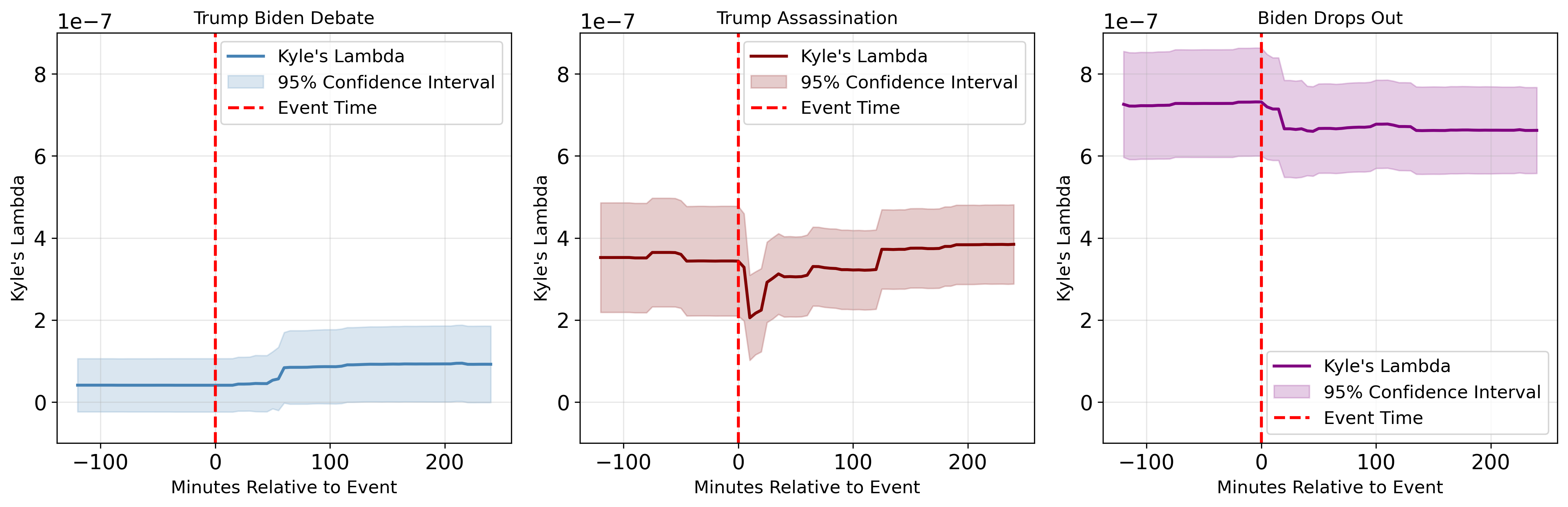

Notes: Panel (a) plots Kyle’s and panel (b) plots the Glosten–Harris permanent (solid) and transitory (dashed) components, both estimated in rolling 5-minute regressions with 95% confidence bands.

Notes: Each panel shows the rolling variance ratio computed from 5-minute log-odds returns with 95% confidence bands; values above one indicate short-horizon drift and values below one indicate short-horizon mean reversion.

Notes: Points show the raw bin-level two-sidedness index and the line is a 15-minute rolling average. Values near one indicate balanced buy/sell pressure (high two-sidedness), while values near zero indicate one-sided flow.
Appendix Online Appendix
This appendix contains five items. Appendix A details the event-study construction used in the main text. Appendix B details the construction of Kyle’s and the Glosten–Harris specification in the binary prediction-market setting. Appendix C reports robustness checks and supplementary specifications, including the matched weekday-time placebo tests. Appendix D reports event-specific panel regressions that are omitted from the main text for brevity. Appendix E reports additional event-time price adjustment plots referenced in the main text.
Appendix A Event-Study Method
This method follows Brown and Warner (1985) and MacKinlay (1997). We conduct an event-study analysis of trading responses around these three events. For each event occurring at time , we reorganize the data into 5-minute event time, , where indexes 5-minute bins relative to the event timestamp.
For each trader , event , and event-time bin , we measure three trading outcomes: trading volume , trading frequency , and an indicator for participation . To accommodate zeros while retaining an approximately log-like scale for large values, we apply the inverse hyperbolic sine transformation to volume and frequency.
(1) Trader-specific baseline (estimation window)
To construct abnormal trading, we estimate each trader’s normal trading activity using an event-specific estimation window prior to the event. Let denote the set of 5-minute bins in the pre-event estimation window. For each trader , we compute baseline volume, frequency, and participation as within-trader means during :
| (4) | ||||||
| (5) | ||||||
We then form transformed baselines and .
(2) Abnormal trading in the event window
Let denote the event window around . We define abnormal trading for each trader and bin as deviations from the trader-specific baseline:
| (6) | ||||
| (7) | ||||
| (8) |
For volume, we additionally set when , so that bins with no trading are treated as having no abnormal activity on the transformed scale.
(3) Aggregation and cumulative abnormal activity
We aggregate abnormal outcomes across traders within each event-time bin. For outcome , the mean abnormal outcome at event time is:
| (9) |
where is the number of trader-bin observations available at . To summarize total post-event responses, we compute cumulative abnormal activity (CAA) as the cumulative sum of bin-level mean abnormal outcomes:
| (10) |
We report confidence intervals for using standard errors computed from the cross-sectional dispersion of within each bin and propagating uncertainty through the cumulative sum under the simplifying assumption of independence across bins:
| (11) | ||||
| (12) |
where is the cross-sectional standard deviation of at event time .
Appendix B Construction of Price-Impact Measures
This section details how Kyle’s is adapted to the setting of a binary prediction market. We estimate Kyle’s for the Trump YES market using detailed trade data.
(1) Infer the direction of transactions
Because we do not observe the full limit order book and only observe matched trades recorded on the Polygon blockchain, we infer trade direction (buyer- versus seller-initiated). We apply a tick-rule classifier: we assign direction , and when the price does not change we carry forward the most recent non-zero direction (Lee and Ready, 1991). We then define signed order flow as:
| (13) |
where is the transaction size in terms of million USDs. This signed volume captures the net demand pressure each transaction places on the market.
(2) Time aggregation
Prediction-market trading is irregular, so to map order flow to price impact consistently we aggregate trades into fixed 5-minute bins in event time. For each bin , we compute the volume-weighted average price (VWAP) and net order flow as:
| (14) |
If no trades occurred in a given bin, we carry forward the last price and set to maintain a continuous time series.
(3) Log-Odds Price Transformation
Because a prediction market price is essentially a probability (Wolfers and Zitzewitz, 2006), and in Polymarket the price is bounded between 0 and 1, price changes are naturally heteroskedastic (e.g. a 5-cent move is more significant when the price is $0.1 vs. when it’s $0.5). To account for this, we convert prices to log-odds to obtain an unbounded metric that is more comparable across different price levels and that mitigates nonlinearity and heteroskedasticity near 0 and 1 (Wolfers and Zitzewitz, 2006):
| (15) |
We then take first differences as our measure of price movement in each 5-minute bin, analogous to a return.
(4) Event-time estimation of price impact
We estimate Kyle’s on 5-minute bins within each event window by regressing log-odds changes on signed order flow:
| (16) |
To separate permanent from transitory effects, we estimate the Glosten–Harris specification:
| (17) |
with HAC standard errors. As an estimate of price impact, is a reduced-form liquidity proxy: larger values indicate lower effective depth, but it does not distinguish informed trading from noise trading. We therefore interpret alongside the permanent/transitory decomposition in event time.
Appendix C Robustness Checks
C.1 Supplementary regression results
| (1) | (2) | (3) | (4) | (5) | (6) | (7) | |
| Baseline | Trading Vol | Trad Int Multi | Trump Holdings | Single Market | Trader Types | Full | |
| Post Event | 0.0039*** | ||||||
| (0.0002) | |||||||
| Post Event Trad Vol High | 0.0110*** | 0.0061*** | |||||
| (0.0006) | (0.0005) | ||||||
| Post Event Trad Int Multi | 0.0145*** | 0.0103*** | |||||
| (0.0009) | (0.0009) | ||||||
| Post Event Neg Trump Win | 0.0066*** | 0.0042*** | |||||
| (0.0006) | (0.0005) | ||||||
| Post Event Single Mkt | -0.0021** | 0.0007 | |||||
| (0.0010) | (0.0010) | ||||||
| Post Event Contrarian | 0.0049** | -0.0046* | |||||
| (0.0024) | (0.0025) | ||||||
| Post Event Momentum | 0.0138*** | 0.0038 | |||||
| (0.0044) | (0.0045) | ||||||
| Entity Effects | YES | YES | YES | YES | YES | YES | YES |
| Time Effects | NO | YES | YES | YES | YES | YES | YES |
| R-Squared (Within) | 0.0017 | 0.0046 | 0.0053 | 0.0024 | -0.0020 | 0.0006 | 0.0063 |
| R-Squared (Between) | 0.0207 | 0.0495 | 0.0575 | 0.0240 | -0.0189 | 0.0059 | 0.0710 |
| R-Squared (Overall) | 0.0040 | 0.0100 | 0.0116 | 0.0050 | -0.0041 | 0.0012 | 0.0141 |
| Observations | 284420 | 284420 | 284420 | 284420 | 284420 | 284420 | 284420 |
-
•
Notes: This table repeats the stacked panel design in Table 5 and Table 6, using a trader-level participation indicator as the dependent variable. The dependent variable equals 1 if the trader trades in a given 5-minute interval and 0 otherwise. Standard errors in parentheses are clustered at the trader-event level. * p0.1, ** p0.05, *** p0.01.
| (1) | (2) | (3) | (4) | (5) | (6) | (7) | |
| Baseline | Trading Vol | Trading Freq | Trump Holdings | Single Market | Trader Types | Full | |
| Post Event | 0.0231*** | 0.0019*** | 0.0063*** | 0.0126*** | 0.0324*** | 0.0215*** | -0.0141** |
| (0.0013) | (0.0004) | (0.0008) | (0.0012) | (0.0059) | (0.0013) | (0.0061) | |
| Trad Vol High | 0.0037*** | 0.0029*** | |||||
| (0.0011) | (0.0007) | ||||||
| Post Event Trad Vol High | 0.0685*** | 0.0453*** | |||||
| (0.0041) | (0.0036) | ||||||
| Trad Freq High | 0.0039*** | 0.0008 | |||||
| (0.0014) | (0.0013) | ||||||
| Post Event Trad Freq High | 0.0703*** | 0.0412*** | |||||
| (0.0048) | (0.0047) | ||||||
| Neg Trump Win | 0.0014 | 0.0006 | |||||
| (0.0009) | (0.0009) | ||||||
| Post Event Neg Trump Win | 0.0339*** | 0.0218*** | |||||
| (0.0034) | (0.0032) | ||||||
| Single Mkt | -0.0028** | -0.0025 | |||||
| (0.0013) | (0.0016) | ||||||
| Post Event Single Mkt | -0.0103* | 0.0069 | |||||
| (0.0061) | (0.0064) | ||||||
| Contrarian | 0.0150 | 0.0130 | |||||
| (0.0092) | (0.0092) | ||||||
| Post Event Contrarian | 0.0324** | -0.0113 | |||||
| (0.0137) | (0.0143) | ||||||
| Momentum | 0.0064** | 0.0041 | |||||
| (0.0031) | (0.0033) | ||||||
| Post Event Momentum | 0.0762** | 0.0308 | |||||
| (0.0303) | (0.0302) | ||||||
| R-squared | 0.0018 | 0.0083 | 0.0077 | 0.0034 | 0.0019 | 0.0026 | 0.0107 |
| R-squared Adj. | 0.0018 | 0.0083 | 0.0076 | 0.0034 | 0.0019 | 0.0026 | 0.0106 |
| Observations | 293,624 | 293,624 | 293,624 | 293,624 | 293,624 | 293,624 | 293,624 |
-
•
Notes: Unit of observation is a trader-by-5-minute bin in the event window, pooled across the three events. The dependent variable is trader-level in event time. Post Event equals 1 for bins at and after the event time. Each column reports an OLS specification with event fixed effects. Regressors include Post Event, the indicated pre-event trader characteristic (Table 3), and its interaction with Post Event. Standard errors are clustered by trader. * p0.1, ** p0.05, *** p0.01.
| (1) | (2) | (3) | (4) | (5) | (6) | (7) | |
| Baseline | Trading Vol | Trading Freq | Trump Holdings | Single Market | Trader Types | Full | |
| Post Event | 0.0042*** | 0.0006*** | 0.0011*** | 0.0020*** | 0.0070*** | 0.0039*** | -0.0017 |
| (0.0003) | (0.0001) | (0.0001) | (0.0002) | (0.0014) | (0.0002) | (0.0013) | |
| Trad Vol High | 0.0007*** | 0.0006*** | |||||
| (0.0002) | (0.0001) | ||||||
| Post Event Trad Vol High | 0.0116*** | 0.0070*** | |||||
| (0.0008) | (0.0007) | ||||||
| Trad Freq High | 0.0007** | 0.0001 | |||||
| (0.0003) | (0.0003) | ||||||
| Post Event Trad Freq High | 0.0129*** | 0.0080*** | |||||
| (0.0009) | (0.0009) | ||||||
| Neg Trump Win | 0.0002 | 0.0001 | |||||
| (0.0002) | (0.0002) | ||||||
| Post Event Neg Trump Win | 0.0070*** | 0.0048*** | |||||
| (0.0007) | (0.0006) | ||||||
| Single Mkt | -0.0008*** | -0.0008** | |||||
| (0.0003) | (0.0004) | ||||||
| Post Event Single Mkt | -0.0032** | 0.0003 | |||||
| (0.0014) | (0.0014) | ||||||
| Contrarian | 0.0025 | 0.0021 | |||||
| (0.0016) | (0.0016) | ||||||
| Post Event Contrarian | 0.0050** | -0.0029 | |||||
| (0.0024) | (0.0025) | ||||||
| Momentum | 0.0010** | 0.0006 | |||||
| (0.0005) | (0.0005) | ||||||
| Post Event Momentum | 0.0149** | 0.0067 | |||||
| (0.0068) | (0.0068) | ||||||
| R-squared | 0.0018 | 0.0075 | 0.0077 | 0.0038 | 0.0021 | 0.0026 | 0.0105 |
| R-squared Adj. | 0.0018 | 0.0075 | 0.0077 | 0.0038 | 0.0021 | 0.0026 | 0.0104 |
| Observations | 293,624 | 293,624 | 293,624 | 293,624 | 293,624 | 293,624 | 293,624 |
-
•
Notes: This table is a repetition of Table C.2, using trader-level as the dependent variable. Standard errors are clustered by trader. * p0.1, ** p0.05, *** p0.01.
| (1) | (2) | (3) | (4) | (5) | (6) | (7) | |
| Baseline | Trading Vol | Trad Int Multi | Trump Holdings | Single Market | Trader Types | Full | |
| Post Event | 0.0040*** | 0.0006*** | 0.0011*** | 0.0019*** | 0.0061*** | 0.0037*** | -0.0016 |
| (0.0002) | (0.0001) | (0.0001) | (0.0002) | (0.0011) | (0.0002) | (0.0010) | |
| Trad Vol High | 0.0007*** | 0.0004*** | |||||
| (0.0002) | (0.0001) | ||||||
| Post Event Trad Vol High | 0.0109*** | 0.0061*** | |||||
| (0.0007) | (0.0005) | ||||||
| Neg Trump Win | 0.0003 | 0.0000 | |||||
| (0.0002) | (0.0002) | ||||||
| Post Event Neg Trump Win | 0.0065*** | 0.0042*** | |||||
| (0.0006) | (0.0005) | ||||||
| Single Mkt | -0.0009*** | -0.0008** | |||||
| (0.0003) | (0.0003) | ||||||
| Post Event Single Mkt | -0.0024** | 0.0004 | |||||
| (0.0011) | (0.0011) | ||||||
| Contrarian | 0.0024 | 0.0018 | |||||
| (0.0015) | (0.0016) | ||||||
| Post Event Contrarian | 0.0049** | -0.0046** | |||||
| (0.0021) | (0.0022) | ||||||
| Momentum | 0.0010* | 0.0003 | |||||
| (0.0005) | (0.0006) | ||||||
| Post Event Momentum | 0.0137** | 0.0038 | |||||
| (0.0059) | (0.0059) | ||||||
| Post Event Trad Int Multi | 0.0144*** | 0.0103*** | |||||
| (0.0010) | (0.0009) | ||||||
| Trad Int Multi | 0.0010*** | 0.0005 | |||||
| (0.0003) | (0.0003) | ||||||
| R-squared | 0.0020 | 0.0082 | 0.0101 | 0.0041 | 0.0023 | 0.0029 | 0.0126 |
| R-squared Adj. | 0.0020 | 0.0082 | 0.0101 | 0.0041 | 0.0022 | 0.0029 | 0.0126 |
| Observations | 293,624 | 293,624 | 293,624 | 293,624 | 293,624 | 293,624 | 293,624 |
-
•
Notes: This table is a repetition of Table C.2, using a trader-level participation indicator as the dependent variable. The dependent variable equals 1 if the trader trades in a given 5-minute interval and 0 otherwise. Standard errors are clustered by trader. * p0.1, ** p0.05, *** p0.01.
C.2 Matched weekday-time placebo tests
To assess whether our event-time patterns could arise by coincidence, we implement matched weekdayclock-time placebo tests. For each real event, we draw 500 pseudo-event timestamps from observed 5-minute bins that share the same weekday and clock time (sampling with replacement), excluding timestamps within hours of any real event. We then recompute the same test statistic at each pseudo-event time and report a two-sided randomization p-value as the share of placebo statistics whose absolute value is at least as large as the real statistic (with a standard +1 finite-sample adjustment).


Notes: Each histogram shows the placebo distribution of the event-time jump in abnormal activity, computed at 500 pseudo-event timestamps matched on weekday and clock time; the dashed vertical line marks the real event value. Panels are arranged as a 3x3 grid with columns for debate/assassination/dropout and rows for volume/frequency/participation. Randomization p-values for these events are: volume 0.012/0.032/0.002; frequency 0.030/0.018/0.002; participation 0.030/0.002/0.002.


Notes: Each histogram shows the placebo distribution of the event-time change in Kyle’s , computed at 500 pseudo-event timestamps matched on weekday and clock time; the dashed vertical line marks the real event value. Randomization p-values are: debate 0.086, assassination 0.002, dropout 0.022.


Notes: Each histogram shows the placebo distribution of the post-event maximum of in the first post-event hour, computed at 500 pseudo-event timestamps matched on weekday and clock time; the dashed vertical line marks the real event value. Real-event maxima and p-values are: debate max (p=0.078), assassination max (p=0.002), dropout max (p=0.675).


Notes: Each histogram shows the placebo distribution of the event-time increase in the two-sidedness index, computed at 500 pseudo-event timestamps matched on weekday and clock time; the dashed vertical line marks the real event value. Randomization p-values are: debate 0.523, assassination 0.014, dropout 0.002.
Appendix D Event-Specific Panel Regressions
| (1) | (2) | (3) | (4) | (5) | (6) | (7) | |
| Baseline | Trading Vol | Trading Freq | Trump Holdings | Single Market | Trader Types | Full | |
| Post Event | 0.0049*** | ||||||
| (0.0012) | |||||||
| Post Event Trad Vol High | 0.0109*** | 0.0077** | |||||
| (0.0036) | (0.0032) | ||||||
| Post Event Trad Freq High | 0.0100** | -0.0043 | |||||
| (0.0043) | (0.0038) | ||||||
| Post Event Neg Trump Win | 0.0189*** | 0.0182*** | |||||
| (0.0035) | (0.0034) | ||||||
| Post Event Single Mkt | -0.0052 | -0.0039 | |||||
| (0.0070) | (0.0076) | ||||||
| Post Event Contrarian | 0.0088 | 0.0092 | |||||
| (0.0168) | (0.0170) | ||||||
| Post Event Momentum | 0.0421** | 0.0433** | |||||
| (0.0171) | (0.0177) | ||||||
| Entity Effects | YES | YES | YES | YES | YES | YES | YES |
| Time Effects | NO | YES | YES | YES | YES | YES | YES |
| R-Squared (Within) | 0.0003 | 0.0005 | 0.0004 | 0.0011 | -0.0007 | 0.0008 | 0.0019 |
| R-Squared (Between) | 0.0059 | 0.0090 | 0.0068 | 0.0114 | -0.0086 | 0.0091 | 0.0204 |
| R-Squared (Overall) | 0.0009 | 0.0015 | 0.0011 | 0.0023 | -0.0017 | 0.0018 | 0.0041 |
| Observations | 71581 | 71581 | 71581 | 71581 | 71581 | 71581 | 71581 |
-
•
Notes: This table reports event-specific panel regressions following the same setting in Table 5. Standard errors in parentheses are clustered by trader. * p0.1, ** p0.05, *** p0.01.
| (1) | (2) | (3) | (4) | (5) | (6) | (7) | |
| Baseline | Trading Vol | Trading Freq | Trump Holdings | Single Market | Trader Types | Full | |
| Post Event | 0.0011*** | ||||||
| (0.0003) | |||||||
| Post Event Trad Vol High | 0.0026*** | 0.0016** | |||||
| (0.0008) | (0.0007) | ||||||
| Post Event Trad Freq High | 0.0030*** | 7.124e-05 | |||||
| (0.0011) | (0.0009) | ||||||
| Post Event Neg Trump Win | 0.0041*** | 0.0039*** | |||||
| (0.0008) | (0.0007) | ||||||
| Post Event Single Mkt | -0.0015 | -0.0010 | |||||
| (0.0021) | (0.0022) | ||||||
| Post Event Contrarian | 0.0029 | 0.0022 | |||||
| (0.0036) | (0.0037) | ||||||
| Post Event Momentum | 0.0089** | 0.0083** | |||||
| (0.0037) | (0.0040) | ||||||
| Entity Effects | YES | YES | YES | YES | YES | YES | YES |
| Time Effects | NO | YES | YES | YES | YES | YES | YES |
| R-Squared (Within) | 0.0003 | 0.0006 | 0.0006 | 0.0012 | -0.0011 | 0.0009 | 0.0020 |
| R-Squared (Between) | 0.0058 | 0.0086 | 0.0087 | 0.0106 | -0.0114 | 0.0092 | 0.0201 |
| R-Squared (Overall) | 0.0009 | 0.0016 | 0.0016 | 0.0024 | -0.0024 | 0.0019 | 0.0043 |
| Observations | 71581 | 71581 | 71581 | 71581 | 71581 | 71581 | 71581 |
-
•
Notes: This table reports event-specific panel regressions following the same setting in Table 6. Standard errors in parentheses are clustered by trader. * p0.1, ** p0.05, *** p0.01.
| (1) | (2) | (3) | (4) | (5) | (6) | (7) | |
| Baseline | Trading Vol | Trad Int Multi | Trump Holdings | Single Market | Trader Types | Full | |
| Post Event | 0.0009*** | ||||||
| (0.0002) | |||||||
| Post Event Trad Vol High | 0.0022*** | 0.0012** | |||||
| (0.0007) | (0.0006) | ||||||
| Post Event Trad Int Multi | 0.0030*** | 0.0001 | |||||
| (0.0010) | (0.0009) | ||||||
| Post Event Neg Trump Win | 0.0038*** | 0.0037*** | |||||
| (0.0007) | (0.0006) | ||||||
| Post Event Single Mkt | -0.0003 | 0.0003 | |||||
| (0.0015) | (0.0015) | ||||||
| Post Event Contrarian | 0.0030 | 0.0023 | |||||
| (0.0032) | (0.0033) | ||||||
| Post Event Momentum | 0.0080*** | 0.0075** | |||||
| (0.0031) | (0.0032) | ||||||
| Entity Effects | YES | YES | YES | YES | YES | YES | YES |
| Time Effects | NO | YES | YES | YES | YES | YES | YES |
| R-Squared (Within) | 0.0003 | 0.0006 | 0.0006 | 0.0012 | -0.0002 | 0.0009 | 0.0017 |
| R-Squared (Between) | 0.0065 | 0.0089 | 0.0100 | 0.0118 | -0.0021 | 0.0104 | 0.0203 |
| R-Squared (Overall) | 0.0010 | 0.0016 | 0.0018 | 0.0025 | -0.0004 | 0.0020 | 0.0039 |
| Observations | 71581 | 71581 | 71581 | 71581 | 71581 | 71581 | 71581 |
-
•
Notes: This table reports event-specific panel regressions following the same setting in Table C.1. Standard errors in parentheses are clustered by trader. * p0.1, ** p0.05, *** p0.01.
| (1) | (2) | (3) | (4) | (5) | (6) | (7) | |
| Baseline | Trading Vol | Trading Freq | Trump Holdings | Single Market | Trader Types | Full | |
| Post Event | 0.0253*** | ||||||
| (0.0023) | |||||||
| Post Event Trad Vol High | 0.0814*** | 0.0697*** | |||||
| (0.0078) | (0.0081) | ||||||
| Post Event Trad Freq High | 0.0682*** | 0.0238** | |||||
| (0.0092) | (0.0100) | ||||||
| Post Event Neg Trump Win | -0.0101** | -0.0231*** | |||||
| (0.0048) | (0.0051) | ||||||
| Post Event Single Mkt | -0.0069 | -0.0033 | |||||
| (0.0093) | (0.0099) | ||||||
| Post Event Contrarian | 0.1477*** | 0.1002** | |||||
| (0.0420) | (0.0412) | ||||||
| Post Event Momentum | 0.1083** | 0.0645 | |||||
| (0.0532) | (0.0527) | ||||||
| Entity Effects | YES | YES | YES | YES | YES | YES | YES |
| Time Effects | NO | YES | YES | YES | YES | YES | YES |
| R-Squared (Within) | 0.0017 | 0.0055 | 0.0035 | -0.0004 | -0.0009 | 0.0014 | 0.0063 |
| R-Squared (Between) | 0.0192 | 0.0572 | 0.0370 | -0.0043 | -0.0094 | 0.0152 | 0.0657 |
| R-Squared (Overall) | 0.0036 | 0.0111 | 0.0072 | -0.0008 | -0.0019 | 0.0029 | 0.0128 |
| Observations | 93200 | 93200 | 93200 | 93200 | 93200 | 93200 | 93200 |
-
•
Notes: This table reports event-specific panel regressions following the same setting in Table 5. Standard errors in parentheses are clustered by trader. * p0.1, ** p0.05, *** p0.01.
| (1) | (2) | (3) | (4) | (5) | (6) | (7) | |
| Baseline | Trading Vol | Trading Freq | Trump Holdings | Single Market | Trader Types | Full | |
| Post Event | 0.0040*** | ||||||
| (0.0004) | |||||||
| Post Event Trad Vol High | 0.0124*** | 0.0098*** | |||||
| (0.0013) | (0.0012) | ||||||
| Post Event Trad Freq High | 0.0118*** | 0.0056*** | |||||
| (0.0016) | (0.0017) | ||||||
| Post Event Neg Trump Win | -0.0012 | -0.0034*** | |||||
| (0.0009) | (0.0009) | ||||||
| Post Event Single Mkt | -0.0016 | -0.0004 | |||||
| (0.0017) | (0.0018) | ||||||
| Post Event Contrarian | 0.0204*** | 0.0122** | |||||
| (0.0061) | (0.0060) | ||||||
| Post Event Momentum | 0.0195* | 0.0119 | |||||
| (0.0107) | (0.0107) | ||||||
| Entity Effects | YES | YES | YES | YES | YES | YES | YES |
| Time Effects | NO | YES | YES | YES | YES | YES | YES |
| R-Squared (Within) | 0.0016 | 0.0048 | 0.0037 | -0.0003 | -0.0013 | 0.0012 | 0.0057 |
| R-Squared (Between) | 0.0183 | 0.0498 | 0.0385 | -0.0031 | -0.0126 | 0.0126 | 0.0588 |
| R-Squared (Overall) | 0.0035 | 0.0098 | 0.0076 | -0.0006 | -0.0026 | 0.0025 | 0.0117 |
| Observations | 93200 | 93200 | 93200 | 93200 | 93200 | 93200 | 93200 |
-
•
Notes: This table reports event-specific panel regressions following the same setting in Table 6. Standard errors in parentheses are clustered by trader. * p0.1, ** p0.05, *** p0.01.
| (1) | (2) | (3) | (4) | (5) | (6) | (7) | |
| Baseline | Trading Vol | Trad Int Multi | Trump Holdings | Single Market | Trader Types | Full | |
| Post Event | 0.0038*** | ||||||
| (0.0003) | |||||||
| Post Event Trad Vol High | 0.0116*** | 0.0089*** | |||||
| (0.0011) | (0.0011) | ||||||
| Post Event Trad Int Multi | 0.0121*** | 0.0061*** | |||||
| (0.0016) | (0.0016) | ||||||
| Post Event Neg Trump Win | -0.0013* | -0.0034*** | |||||
| (0.0007) | (0.0007) | ||||||
| Post Event Single Mkt | -0.0011 | -0.0005 | |||||
| (0.0015) | (0.0015) | ||||||
| Post Event Contrarian | 0.0207*** | 0.0124** | |||||
| (0.0059) | (0.0058) | ||||||
| Post Event Momentum | 0.0195* | 0.0117 | |||||
| (0.0103) | (0.0103) | ||||||
| Entity Effects | YES | YES | YES | YES | YES | YES | YES |
| Time Effects | NO | YES | YES | YES | YES | YES | YES |
| R-Squared (Within) | 0.0018 | 0.0051 | 0.0040 | -0.0004 | -0.0010 | 0.0015 | 0.0062 |
| R-Squared (Between) | 0.0215 | 0.0574 | 0.0463 | -0.0041 | -0.0105 | 0.0164 | 0.0694 |
| R-Squared (Overall) | 0.0039 | 0.0108 | 0.0086 | -0.0008 | -0.0020 | 0.0031 | 0.0130 |
| Observations | 93200 | 93200 | 93200 | 93200 | 93200 | 93200 | 93200 |
-
•
Notes: This table reports event-specific panel regressions following the same setting in Table C.1. Standard errors in parentheses are clustered by trader. * p0.1, ** p0.05, *** p0.01.
| (1) | (2) | (3) | (4) | (5) | (6) | (7) | |
| Baseline | Trading Vol | Trading Freq | Trump Holdings | Single Market | Trader Types | Full | |
| Post Event | 0.0321*** | ||||||
| (0.0023) | |||||||
| Post Event Trad Vol High | 0.0923*** | 0.0479*** | |||||
| (0.0070) | (0.0054) | ||||||
| Post Event Trad Freq High | 0.1015*** | 0.0625*** | |||||
| (0.0079) | (0.0069) | ||||||
| Post Event Neg Trump Win | 0.0787*** | 0.0612*** | |||||
| (0.0069) | (0.0062) | ||||||
| Post Event Single Mkt | -0.0129 | 0.0251** | |||||
| (0.0100) | (0.0105) | ||||||
| Post Event Contrarian | -0.0167 | -0.0499* | |||||
| (0.0259) | (0.0285) | ||||||
| Post Event Momentum | 0.1711** | 0.1250 | |||||
| (0.0871) | (0.0855) | ||||||
| Entity Effects | YES | YES | YES | YES | YES | YES | YES |
| Time Effects | NO | YES | YES | YES | YES | YES | YES |
| R-Squared (Within) | 0.0023 | 0.0065 | 0.0069 | 0.0051 | -0.0019 | 0.0007 | 0.0059 |
| R-Squared (Between) | 0.0252 | 0.0670 | 0.0700 | 0.0506 | -0.0176 | 0.0052 | 0.0743 |
| R-Squared (Overall) | 0.0051 | 0.0141 | 0.0148 | 0.0108 | -0.0039 | 0.0012 | 0.0144 |
| Observations | 119639 | 119639 | 119639 | 119639 | 119639 | 119639 | 119639 |
-
•
Notes: This table reports event-specific panel regressions following the same setting in Table 5. Standard errors in parentheses are clustered by trader. * p0.1, ** p0.05, *** p0.01.
| (1) | (2) | (3) | (4) | (5) | (6) | (7) | |
| Baseline | Trading Vol | Trading Freq | Trump Holdings | Single Market | Trader Types | Full | |
| Post Event | 0.0061*** | ||||||
| (0.0005) | |||||||
| Post Event Trad Vol High | 0.0162*** | 0.0080*** | |||||
| (0.0014) | (0.0012) | ||||||
| Post Event Trad Freq High | 0.0185*** | 0.0113*** | |||||
| (0.0016) | (0.0015) | ||||||
| Post Event Neg Trump Win | 0.0154*** | 0.0121*** | |||||
| (0.0014) | (0.0012) | ||||||
| Post Event Single Mkt | -0.0048** | 0.0024 | |||||
| (0.0024) | (0.0024) | ||||||
| Post Event Contrarian | -0.0025 | -0.0084* | |||||
| (0.0038) | (0.0043) | ||||||
| Post Event Momentum | 0.0330* | 0.0245 | |||||
| (0.0186) | (0.0183) | ||||||
| Entity Effects | YES | YES | YES | YES | YES | YES | YES |
| Time Effects | NO | YES | YES | YES | YES | YES | YES |
| R-Squared (Within) | 0.0024 | 0.0061 | 0.0067 | 0.0055 | -0.0044 | 0.0007 | 0.0078 |
| R-Squared (Between) | 0.0222 | 0.0537 | 0.0585 | 0.0464 | -0.0337 | 0.0048 | 0.0748 |
| R-Squared (Overall) | 0.0052 | 0.0130 | 0.0142 | 0.0114 | -0.0086 | 0.0013 | 0.0175 |
| Observations | 119639 | 119639 | 119639 | 119639 | 119639 | 119639 | 119639 |
-
•
Notes: This table reports event-specific panel regressions following the same setting in Table 6. Standard errors in parentheses are clustered by trader. * p0.1, ** p0.05, *** p0.01.
| (1) | (2) | (3) | (4) | (5) | (6) | (7) | |
| Baseline | Trading Vol | Trad Int Multi | Trump Holdings | Single Market | Trader Types | Full | |
| Post Event | 0.0058*** | ||||||
| (0.0004) | |||||||
| Post Event Trad Vol High | 0.0155*** | 0.0067*** | |||||
| (0.0011) | (0.0008) | ||||||
| Post Event Trad Int Multi | 0.0213*** | 0.0149*** | |||||
| (0.0016) | (0.0014) | ||||||
| Post Event Neg Trump Win | 0.0146*** | 0.0109*** | |||||
| (0.0012) | (0.0010) | ||||||
| Post Event Single Mkt | -0.0038** | 0.0026 | |||||
| (0.0019) | (0.0018) | ||||||
| Post Event Contrarian | -0.0040* | -0.0117*** | |||||
| (0.0021) | (0.0028) | ||||||
| Post Event Momentum | 0.0296* | 0.0189 | |||||
| (0.0154) | (0.0151) | ||||||
| Entity Effects | YES | YES | YES | YES | YES | YES | YES |
| Time Effects | NO | YES | YES | YES | YES | YES | YES |
| R-Squared (Within) | 0.0026 | 0.0066 | 0.0086 | 0.0060 | -0.0039 | 0.0007 | 0.0092 |
| R-Squared (Between) | 0.0284 | 0.0681 | 0.0879 | 0.0584 | -0.0346 | 0.0053 | 0.1037 |
| R-Squared (Overall) | 0.0059 | 0.0145 | 0.0188 | 0.0127 | -0.0078 | 0.0013 | 0.0213 |
| Observations | 119639 | 119639 | 119639 | 119639 | 119639 | 119639 | 119639 |
-
•
Notes: This table reports event-specific panel regressions following the same setting in Table C.1. Standard errors in parentheses are clustered by trader. * p0.1, ** p0.05, *** p0.01.
| (1) | (2) | (3) | (4) | (5) | (6) | (7) | |
| Baseline | Trading Vol | Trading Freq | Trump Holdings | Single Market | Trader Types | Full | |
| Post Event | 0.0050*** | 0.0017* | 0.0029*** | -0.0009 | 0.0106* | 0.0033*** | 0.0008 |
| (0.0012) | (0.0009) | (0.0010) | (0.0009) | (0.0064) | (0.0010) | (0.0065) | |
| Trad Vol High | 0.0024 | 0.0026* | |||||
| (0.0020) | (0.0015) | ||||||
| Post Event Trad Vol High | 0.0107*** | 0.0077** | |||||
| (0.0034) | (0.0031) | ||||||
| Trad Freq High | 0.0030 | -0.0007 | |||||
| (0.0027) | (0.0017) | ||||||
| Post Event Trad Freq High | 0.0099** | -0.0047 | |||||
| (0.0042) | (0.0036) | ||||||
| Neg Trump Win | -0.0016 | -0.0026* | |||||
| (0.0011) | (0.0014) | ||||||
| Post Event Neg Trump Win | 0.0188*** | 0.0180*** | |||||
| (0.0034) | (0.0032) | ||||||
| Single Mkt | -0.0057* | -0.0070** | |||||
| (0.0032) | (0.0036) | ||||||
| Post Event Single Mkt | -0.0062 | -0.0051 | |||||
| (0.0065) | (0.0070) | ||||||
| Contrarian | 0.0149 | 0.0150 | |||||
| (0.0161) | (0.0161) | ||||||
| Post Event Contrarian | 0.0087 | 0.0095 | |||||
| (0.0161) | (0.0163) | ||||||
| Momentum | -0.0013*** | -0.0013 | |||||
| (0.0005) | (0.0017) | ||||||
| Post Event Momentum | 0.0420** | 0.0435** | |||||
| (0.0164) | (0.0170) | ||||||
| R-squared | 0.0003 | 0.0011 | 0.0009 | 0.0016 | 0.0006 | 0.0019 | 0.0039 |
| R-squared Adj. | 0.0002 | 0.0010 | 0.0009 | 0.0016 | 0.0005 | 0.0018 | 0.0037 |
| Observations | 71,581 | 71,581 | 71,581 | 71,581 | 71,581 | 71,581 | 71,581 |
-
•
Notes: This table reports event-specific OLS regressions following the same setting in Table C.2. Standard errors in parentheses are clustered by trader. * p0.1, ** p0.05, *** p0.01.
| (1) | (2) | (3) | (4) | (5) | (6) | (7) | |
| Baseline | Trading Vol | Trading Freq | Trump Holdings | Single Market | Trader Types | Full | |
| Post Event | 0.0011*** | 0.0003* | 0.0005** | -0.0002 | 0.0029 | 0.0007*** | 0.0004 |
| (0.0003) | (0.0002) | (0.0002) | (0.0002) | (0.0019) | (0.0002) | (0.0018) | |
| Trad Vol High | 0.0003 | 0.0005* | |||||
| (0.0004) | (0.0003) | ||||||
| Post Event Trad Vol High | 0.0025*** | 0.0016** | |||||
| (0.0008) | (0.0007) | ||||||
| Trad Freq High | 0.0004 | -0.0004 | |||||
| (0.0005) | (0.0003) | ||||||
| Post Event Trad Freq High | 0.0029*** | -0.0001 | |||||
| (0.0010) | (0.0009) | ||||||
| Neg Trump Win | -0.0004* | -0.0006** | |||||
| (0.0002) | (0.0003) | ||||||
| Post Event Neg Trump Win | 0.0041*** | 0.0038*** | |||||
| (0.0008) | (0.0006) | ||||||
| Single Mkt | -0.0016** | -0.0020** | |||||
| (0.0008) | (0.0009) | ||||||
| Post Event Single Mkt | -0.0019 | -0.0015 | |||||
| (0.0019) | (0.0020) | ||||||
| Contrarian | 0.0027 | 0.0030 | |||||
| (0.0030) | (0.0030) | ||||||
| Post Event Contrarian | 0.0028 | 0.0023 | |||||
| (0.0035) | (0.0035) | ||||||
| Momentum | -0.0003*** | -0.0000 | |||||
| (0.0001) | (0.0003) | ||||||
| Post Event Momentum | 0.0088** | 0.0084** | |||||
| (0.0036) | (0.0038) | ||||||
| R-squared | 0.0003 | 0.0011 | 0.0012 | 0.0017 | 0.0009 | 0.0019 | 0.0042 |
| R-squared Adj. | 0.0003 | 0.0010 | 0.0012 | 0.0016 | 0.0009 | 0.0018 | 0.0040 |
| Observations | 71,581 | 71,581 | 71,581 | 71,581 | 71,581 | 71,581 | 71,581 |
-
•
Notes: This table reports event-specific OLS regressions following the same setting in Table C.3. Standard errors in parentheses are clustered by trader. * p0.1, ** p0.05, *** p0.01.
| (1) | (2) | (3) | (4) | (5) | (6) | (7) | |
| Baseline | Trading Vol | Trad Int Multi | Trump Holdings | Single Market | Trader Types | Full | |
| Post Event | 0.0010*** | 0.0003* | 0.0005** | -0.0002 | 0.0016 | 0.0006*** | -0.0007 |
| (0.0002) | (0.0002) | (0.0002) | (0.0002) | (0.0013) | (0.0002) | (0.0013) | |
| Trad Vol High | 0.0003 | 0.0003 | |||||
| (0.0004) | (0.0002) | ||||||
| Post Event Trad Vol High | 0.0021*** | 0.0012** | |||||
| (0.0006) | (0.0005) | ||||||
| Trad Int Multi | 0.0006 | 0.0001 | |||||
| (0.0006) | (0.0004) | ||||||
| Post Event Trad Int Multi | 0.0029*** | 0.0001 | |||||
| (0.0010) | (0.0008) | ||||||
| Neg Trump Win | -0.0004* | -0.0006** | |||||
| (0.0002) | (0.0003) | ||||||
| Post Event Neg Trump Win | 0.0037*** | 0.0036*** | |||||
| (0.0006) | (0.0006) | ||||||
| Single Mkt | -0.0017** | -0.0019** | |||||
| (0.0008) | (0.0008) | ||||||
| Post Event Single Mkt | -0.0007 | -0.0001 | |||||
| (0.0013) | (0.0014) | ||||||
| Contrarian | 0.0025 | 0.0024 | |||||
| (0.0028) | (0.0028) | ||||||
| Post Event Contrarian | 0.0030 | 0.0024 | |||||
| (0.0031) | (0.0032) | ||||||
| Momentum | -0.0003*** | -0.0004 | |||||
| (0.0001) | (0.0004) | ||||||
| Post Event Momentum | 0.0079*** | 0.0075** | |||||
| (0.0029) | (0.0031) | ||||||
| R-squared | 0.0003 | 0.0010 | 0.0014 | 0.0017 | 0.0007 | 0.0020 | 0.0041 |
| R-squared Adj. | 0.0003 | 0.0010 | 0.0013 | 0.0017 | 0.0006 | 0.0019 | 0.0039 |
| Observations | 71,581 | 71,581 | 71,581 | 71,581 | 71,581 | 71,581 | 71,581 |
-
•
Notes: This table reports event-specific OLS regressions following the same setting in Table C.4. Standard errors in parentheses are clustered by trader. * p0.1, ** p0.05, *** p0.01.
| (1) | (2) | (3) | (4) | (5) | (6) | (7) | |
| Baseline | Trading Vol | Trading Freq | Trump Holdings | Single Market | Trader Types | Full | |
| Post Event | 0.0254*** | 0.0017*** | 0.0110*** | 0.0286*** | 0.0323*** | 0.0224*** | 0.0094 |
| (0.0023) | (0.0006) | (0.0016) | (0.0028) | (0.0084) | (0.0022) | (0.0090) | |
| Trad Vol High | 0.0017 | 0.0014* | |||||
| (0.0012) | (0.0008) | ||||||
| Post Event Trad Vol High | 0.0813*** | 0.0697*** | |||||
| (0.0075) | (0.0078) | ||||||
| Trad Freq High | 0.0018 | 0.0003 | |||||
| (0.0015) | (0.0015) | ||||||
| Post Event Trad Freq High | 0.0681*** | 0.0236** | |||||
| (0.0088) | (0.0096) | ||||||
| Neg Trump Win | 0.0003 | -0.0002 | |||||
| (0.0008) | (0.0009) | ||||||
| Post Event Neg Trump Win | -0.0102** | -0.0233*** | |||||
| (0.0046) | (0.0048) | ||||||
| Single Mkt | -0.0023 | -0.0021 | |||||
| (0.0018) | (0.0021) | ||||||
| Post Event Single Mkt | -0.0077 | -0.0042 | |||||
| (0.0087) | (0.0093) | ||||||
| Contrarian | -0.0007** | -0.0014 | |||||
| (0.0004) | (0.0014) | ||||||
| Post Event Contrarian | 0.1476*** | 0.1004** | |||||
| (0.0404) | (0.0396) | ||||||
| Momentum | 0.0128 | 0.0119 | |||||
| (0.0134) | (0.0134) | ||||||
| Post Event Momentum | 0.1082** | 0.0645 | |||||
| (0.0511) | (0.0506) | ||||||
| R-squared | 0.0016 | 0.0091 | 0.0059 | 0.0017 | 0.0016 | 0.0037 | 0.0112 |
| R-squared Adj. | 0.0016 | 0.0091 | 0.0058 | 0.0017 | 0.0016 | 0.0037 | 0.0111 |
| Observations | 93,200 | 93,200 | 93,200 | 93,200 | 93,200 | 93,200 | 93,200 |
-
•
Notes: This table reports event-specific OLS regressions following the same setting in Table C.2. Standard errors in parentheses are clustered by trader. * p0.1, ** p0.05, *** p0.01.
| (1) | (2) | (3) | (4) | (5) | (6) | (7) | |
| Baseline | Trading Vol | Trading Freq | Trump Holdings | Single Market | Trader Types | Full | |
| Post Event | 0.0040*** | 0.0004*** | 0.0016*** | 0.0045*** | 0.0056*** | 0.0036*** | 0.0015 |
| (0.0004) | (0.0001) | (0.0002) | (0.0004) | (0.0016) | (0.0004) | (0.0016) | |
| Trad Vol High | 0.0004 | 0.0003* | |||||
| (0.0003) | (0.0002) | ||||||
| Post Event Trad Vol High | 0.0124*** | 0.0097*** | |||||
| (0.0012) | (0.0012) | ||||||
| Trad Freq High | 0.0005 | 0.0001 | |||||
| (0.0003) | (0.0004) | ||||||
| Post Event Trad Freq High | 0.0117*** | 0.0055*** | |||||
| (0.0015) | (0.0016) | ||||||
| Neg Trump Win | 0.0001 | -0.0001 | |||||
| (0.0002) | (0.0002) | ||||||
| Post Event Neg Trump Win | -0.0013 | -0.0034*** | |||||
| (0.0008) | (0.0008) | ||||||
| Single Mkt | -0.0007 | -0.0007 | |||||
| (0.0005) | (0.0005) | ||||||
| Post Event Single Mkt | -0.0018 | -0.0007 | |||||
| (0.0016) | (0.0017) | ||||||
| Contrarian | -0.0002** | -0.0004 | |||||
| (0.0001) | (0.0003) | ||||||
| Post Event Contrarian | 0.0203*** | 0.0122** | |||||
| (0.0058) | (0.0058) | ||||||
| Momentum | 0.0018 | 0.0015 | |||||
| (0.0020) | (0.0020) | ||||||
| Post Event Momentum | 0.0194* | 0.0119 | |||||
| (0.0103) | (0.0103) | ||||||
| R-squared | 0.0014 | 0.0079 | 0.0062 | 0.0015 | 0.0016 | 0.0033 | 0.0101 |
| R-squared Adj. | 0.0014 | 0.0079 | 0.0062 | 0.0015 | 0.0015 | 0.0032 | 0.0099 |
| Observations | 93,200 | 93,200 | 93,200 | 93,200 | 93,200 | 93,200 | 93,200 |
-
•
Notes: This table reports event-specific OLS regressions following the same setting in Table C.3. Standard errors in parentheses are clustered by trader. * p0.1, ** p0.05, *** p0.01.
| (1) | (2) | (3) | (4) | (5) | (6) | (7) | |
| Baseline | Trading Vol | Trad Int Multi | Trump Holdings | Single Market | Trader Types | Full | |
| Post Event | 0.0038*** | 0.0005*** | 0.0017*** | 0.0043*** | 0.0050*** | 0.0034*** | 0.0017 |
| (0.0003) | (0.0001) | (0.0002) | (0.0004) | (0.0014) | (0.0003) | (0.0013) | |
| Trad Vol High | 0.0005 | 0.0003 | |||||
| (0.0003) | (0.0002) | ||||||
| Post Event Trad Vol High | 0.0116*** | 0.0089*** | |||||
| (0.0011) | (0.0010) | ||||||
| Trad Int Multi | 0.0007 | 0.0004 | |||||
| (0.0005) | (0.0005) | ||||||
| Post Event Trad Int Multi | 0.0121*** | 0.0061*** | |||||
| (0.0015) | (0.0016) | ||||||
| Neg Trump Win | 0.0001 | -0.0001 | |||||
| (0.0002) | (0.0002) | ||||||
| Post Event Neg Trump Win | -0.0014* | -0.0035*** | |||||
| (0.0007) | (0.0007) | ||||||
| Single Mkt | -0.0007 | -0.0006 | |||||
| (0.0004) | (0.0005) | ||||||
| Post Event Single Mkt | -0.0013 | -0.0008 | |||||
| (0.0014) | (0.0014) | ||||||
| Contrarian | -0.0002** | -0.0006 | |||||
| (0.0001) | (0.0005) | ||||||
| Post Event Contrarian | 0.0207*** | 0.0124** | |||||
| (0.0057) | (0.0056) | ||||||
| Momentum | 0.0020 | 0.0016 | |||||
| (0.0022) | (0.0023) | ||||||
| Post Event Momentum | 0.0195* | 0.0117 | |||||
| (0.0099) | (0.0099) | ||||||
| R-squared | 0.0016 | 0.0086 | 0.0072 | 0.0017 | 0.0017 | 0.0039 | 0.0115 |
| R-squared Adj. | 0.0016 | 0.0086 | 0.0072 | 0.0016 | 0.0017 | 0.0038 | 0.0114 |
| Observations | 93,200 | 93,200 | 93,200 | 93,200 | 93,200 | 93,200 | 93,200 |
-
•
Notes: This table reports event-specific OLS regressions following the same setting in Table C.4. Standard errors in parentheses are clustered by trader. * p0.1, ** p0.05, *** p0.01.
| (1) | (2) | (3) | (4) | (5) | (6) | (7) | |
| Baseline | Trading Vol | Trading Freq | Trump Holdings | Single Market | Trader Types | Full | |
| Post Event | 0.0322*** | 0.0022*** | 0.0045*** | 0.0083*** | 0.0447*** | 0.0311*** | -0.0409*** |
| (0.0023) | (0.0007) | (0.0011) | (0.0015) | (0.0092) | (0.0022) | (0.0098) | |
| Trad Vol High | 0.0062*** | 0.0038*** | |||||
| (0.0021) | (0.0014) | ||||||
| Post Event Trad Vol High | 0.0921*** | 0.0479*** | |||||
| (0.0067) | (0.0052) | ||||||
| Trad Freq High | 0.0066*** | 0.0037* | |||||
| (0.0024) | (0.0022) | ||||||
| Post Event Trad Freq High | 0.1013*** | 0.0621*** | |||||
| (0.0076) | (0.0067) | ||||||
| Neg Trump Win | 0.0040** | 0.0027 | |||||
| (0.0020) | (0.0019) | ||||||
| Post Event Neg Trump Win | 0.0785*** | 0.0609*** | |||||
| (0.0066) | (0.0059) | ||||||
| Single Mkt | -0.0019 | -0.0000 | |||||
| (0.0020) | (0.0027) | ||||||
| Post Event Single Mkt | -0.0139 | 0.0237** | |||||
| (0.0094) | (0.0099) | ||||||
| Contrarian | 0.0141 | 0.0121 | |||||
| (0.0166) | (0.0166) | ||||||
| Post Event Contrarian | -0.0169 | -0.0499* | |||||
| (0.0249) | (0.0274) | ||||||
| Momentum | -0.0026*** | -0.0057*** | |||||
| (0.0007) | (0.0018) | ||||||
| Post Event Momentum | 0.1710** | 0.1249 | |||||
| (0.0836) | (0.0822) | ||||||
| R-squared | 0.0020 | 0.0111 | 0.0119 | 0.0082 | 0.0021 | 0.0029 | 0.0181 |
| R-squared Adj. | 0.0020 | 0.0111 | 0.0119 | 0.0082 | 0.0021 | 0.0029 | 0.0180 |
| Observations | 119,639 | 119,639 | 119,639 | 119,639 | 119,639 | 119,639 | 119,639 |
-
•
Notes: This table reports event-specific OLS regressions following the same setting in Table C.2. Standard errors in parentheses are clustered by trader. * p0.1, ** p0.05, *** p0.01.
| (1) | (2) | (3) | (4) | (5) | (6) | (7) | |
| Baseline | Trading Vol | Trading Freq | Trump Holdings | Single Market | Trader Types | Full | |
| Post Event | 0.0061*** | 0.0008*** | 0.0010*** | 0.0014*** | 0.0105*** | 0.0059*** | -0.0053** |
| (0.0005) | (0.0002) | (0.0002) | (0.0003) | (0.0022) | (0.0004) | (0.0021) | |
| Trad Vol High | 0.0012*** | 0.0007** | |||||
| (0.0004) | (0.0003) | ||||||
| Post Event Trad Vol High | 0.0162*** | 0.0080*** | |||||
| (0.0013) | (0.0011) | ||||||
| Trad Freq High | 0.0012** | 0.0007 | |||||
| (0.0005) | (0.0005) | ||||||
| Post Event Trad Freq High | 0.0185*** | 0.0112*** | |||||
| (0.0015) | (0.0014) | ||||||
| Neg Trump Win | 0.0007* | 0.0005 | |||||
| (0.0004) | (0.0004) | ||||||
| Post Event Neg Trump Win | 0.0154*** | 0.0121*** | |||||
| (0.0014) | (0.0012) | ||||||
| Single Mkt | -0.0004 | -0.0001 | |||||
| (0.0004) | (0.0005) | ||||||
| Post Event Single Mkt | -0.0050** | 0.0021 | |||||
| (0.0023) | (0.0022) | ||||||
| Contrarian | 0.0015 | 0.0011 | |||||
| (0.0020) | (0.0020) | ||||||
| Post Event Contrarian | -0.0026 | -0.0083** | |||||
| (0.0036) | (0.0041) | ||||||
| Momentum | -0.0005*** | -0.0011*** | |||||
| (0.0001) | (0.0004) | ||||||
| Post Event Momentum | 0.0330* | 0.0245 | |||||
| (0.0179) | (0.0176) | ||||||
| R-squared | 0.0021 | 0.0101 | 0.0114 | 0.0087 | 0.0024 | 0.0030 | 0.0175 |
| R-squared Adj. | 0.0021 | 0.0101 | 0.0114 | 0.0087 | 0.0024 | 0.0030 | 0.0174 |
| Observations | 119,639 | 119,639 | 119,639 | 119,639 | 119,639 | 119,639 | 119,639 |
-
•
Notes: This table reports event-specific OLS regressions following the same setting in Table C.3. Standard errors in parentheses are clustered by trader. * p0.1, ** p0.05, *** p0.01.
| (1) | (2) | (3) | (4) | (5) | (6) | (7) | |
| Baseline | Trading Vol | Trad Int Multi | Trump Holdings | Single Market | Trader Types | Full | |
| Post Event | 0.0058*** | 0.0008*** | 0.0011*** | 0.0014*** | 0.0095*** | 0.0056*** | -0.0052*** |
| (0.0004) | (0.0002) | (0.0002) | (0.0002) | (0.0017) | (0.0004) | (0.0017) | |
| Trad Vol High | 0.0012*** | 0.0006** | |||||
| (0.0004) | (0.0002) | ||||||
| Post Event Trad Vol High | 0.0154*** | 0.0067*** | |||||
| (0.0011) | (0.0008) | ||||||
| Trad Int Multi | 0.0016*** | 0.0011** | |||||
| (0.0006) | (0.0005) | ||||||
| Post Event Trad Int Multi | 0.0213*** | 0.0149*** | |||||
| (0.0015) | (0.0013) | ||||||
| Neg Trump Win | 0.0008* | 0.0004 | |||||
| (0.0004) | (0.0004) | ||||||
| Post Event Neg Trump Win | 0.0146*** | 0.0108*** | |||||
| (0.0011) | (0.0010) | ||||||
| Single Mkt | -0.0006 | -0.0002 | |||||
| (0.0005) | (0.0006) | ||||||
| Post Event Single Mkt | -0.0041** | 0.0024 | |||||
| (0.0018) | (0.0017) | ||||||
| Contrarian | 0.0018 | 0.0012 | |||||
| (0.0023) | (0.0023) | ||||||
| Post Event Contrarian | -0.0040* | -0.0117*** | |||||
| (0.0020) | (0.0027) | ||||||
| Momentum | -0.0005*** | -0.0014*** | |||||
| (0.0001) | (0.0005) | ||||||
| Post Event Momentum | 0.0296** | 0.0188 | |||||
| (0.0148) | (0.0145) | ||||||
| R-squared | 0.0023 | 0.0113 | 0.0157 | 0.0097 | 0.0026 | 0.0032 | 0.0215 |
| R-squared Adj. | 0.0023 | 0.0112 | 0.0157 | 0.0096 | 0.0026 | 0.0032 | 0.0214 |
| Observations | 119,639 | 119,639 | 119,639 | 119,639 | 119,639 | 119,639 | 119,639 |
-
•
Notes: This table reports event-specific OLS regressions following the same setting in Table C.4. Standard errors in parentheses are clustered by trader. * p0.1, ** p0.05, *** p0.01.
Appendix E Additional Event-Time Price Adjustment Plots
This appendix reports supplementary price adjustment plots referenced in Section 5. Unless otherwise noted, all figures use 5-minute event time in a 2-hour pre / 4-hour post window around each event.


Notes: In this plot, each panel plots the 5-minute volume-weighted average transaction price (line) and trading volume (bars) in the event window (-2h, +4h).


Notes: In this plot, each panel plots the 5-minute volume-weighted average transaction price (line) and trading volume (bars) in the event window (-2h, +4h).