eTFCE: Exact Threshold-Free Cluster Enhancement via Fast Cluster Retrieval

Abstract

Threshold-free cluster enhancement (TFCE) is a popular method for cluster extent inference but is computationally intensive. Existing TFCE implementations often rely on discretized approximation that introduces numerical errors. Also, we identified a long-standing scaling error in the FSL implementation of TFCE (version 6.0.7.19 and earlier). As an alternative implementation, we present eTFCE, an efficient framework that computes exact TFCE scores using an optimized cluster retrieval algorithm, which, though exact, reduces computation time by approximately $50\%$ compared to standard approximated implementations. In addition, the proposed framework enables simultaneous computation of TFCE and generalized cluster statistics, formulated similarly to TFCE, within a single nonparametric run, with negligible additional computational cost. This, in turn, facilitates systematic method comparisons, and enables a more complete characterization of spatial activation patterns. As a result, eTFCE establishes a mathematically exact and computationally efficient framework for comprehensive and informative nonparametric inference in neuroimaging.

1 Introduction

In neuroimaging, traditional cluster extent inference suffers from issues of dependence on arbitrarily chosen cluster defining thresholds (CDTs) and low spatial specificity (Woo2014; Eklund2016; Rosenblatt2018). Threshold-free cluster enhancement (TFCE) claims to eliminate the need to select an arbitrary CDT by integrating cluster-extent information and voxel-wise statistic height across all possible threshold levels (Smith2009; Salimi-Khorshidi2011). However, the TFCE analysis process, especially when embedded within a nonparametric permutation testing framework, makes TFCE computationally intensive, presenting a serious challenge for large-scale studies (Nichols2002; Winkler2014).

This paper tackles the challenges of computational efficiency and numerical accuracy by introducing an exact and efficient TFCE implementation (eTFCE). The standard approach to make TFCE feasible in practice involves a computational approximation. The TFCE integral is discretized over a fixed set of CDT levels (e.g., $100$ equally spaced CDTs in FSL (Jenkinson2012)) to avoid the cost of an exact calculation. However, this common approximation introduces two critical issues. First, the discretization sacrifices mathematical exactness by considering only a small number of CDTs. Second, as we identified, the implementation in widely used tools like FSL contains a scaling error that further distorts the results. These issues reveal the deficiency of fixed-step approximations and motivate our development of a method that is both exact and computationally efficient.

Our key insight is that the TFCE integral can be computed more efficiently than previously assumed using the optimized cluster retrieval algorithm, which largely eliminates the need for error-prone approximations (Chen2023). eTFCE produces mathematically exact and numerically consistent results while requiring only around $50\%$ of the computation time of the common approximate implementation in FSL. This reverses the traditional trade-off. Instead of sacrificing accuracy for speed, researchers can achieve higher accuracy with improved efficiency. The combination of consistent time savings and mathematical exactness makes eTFCE a strong candidate as a practical default, supporting more accessible and reliable nonparametric inference.

Furthermore, the integrated design of eTFCE enables efficient computation of multiple cluster-based statistics (e.g., traditional cluster extent, and cluster mass) together with the TFCE scores within the same nonparametric framework, at minimal additional cost. It allows researchers to obtain both TFCE-based and cluster-wise inference results directly from a single analysis run. This also demonstrates the generality of the underlying computational framework, which is applicable to a broader family of methods that share the generalized formulation and face similar computational constraints.

2 Background

In this section, we briefly review two key components: the TFCE score and the cluster retrieval algorithm.

2.1 Threshold-Free Cluster Enhancement (TFCE)

The TFCE score at voxel $v$ in the brain volume $\mathcal{B}$ is defined as

$$\text{TFCE}(v)=\int_{h_{0}}^{h_{v}}e_{v}(h)^{E}h^{H}\,dh,$$ (1)

where $h$ denotes the chosen CDT level ranging from $h_{0}$ (typically set to $0$) to the voxel height $h_{v}$, $e_{v}(h)$ is the size of the cluster, thresholded at level $h$, that contains voxel $v$, and $E$ and $H$ are the extent and height parameters, respectively. Smith2009 recommended $E=0.5$ and $H=2$ for 3D space.

While the TFCE score is defined by the integral (1), common implementations, including the default in FSL, approximate it through discretization over a sequence of non-decreasing CDTs $\{\tau_{i}\}_{i=1}^{n}$. Here, the number of thresholds $n$ determines the step size of the approximation. This yields a general discrete approximation of the TFCE score:

$$\text{TFCE}(v)\approx\sum_{i=1}^{n}e_{v}(\tau_{i})^{E}\tau_{i}^{H}\Delta\tau_{i},$$ (2)

where $\Delta\tau_{i}$ represents the local step size associated with $\tau_{i}$. Typically, equally spaced thresholds ($\Delta\tau_{i}=\Delta\tau$) are used with $n$ set to a relatively small number for computational efficiency, which can introduce a relatively large approximation error.

The default threshold selection strategy implemented in FSL’s randomise and fslmaths implementation (FSL version 6.0.7.19; Jenkinson2012) utilizes a uniform sequence of $n=100$ thresholds from $0$ to $h_{\max}$. Given $n$, a constant step size is automatically determined as $\Delta\tau=h_{\max}/n$, where $h_{\max}$ is the maximum voxel height in $\mathcal{B}$. The TFCE scores are then computed independently for each voxel, with the cluster sizes evaluated separately at each threshold $\tau_{i}$.

However, a numerical error exists in the current TFCE computation within FSL (observed in version 6.0.7.19 and earlier). The implementation calculates $\sum_{i=1}^{n}e_{v}(\tau_{i})^{E}\tau_{i}^{H}$, which is incorrect as it omits the step size $\Delta\tau$ from the discrete approximation of the integral (see Equation (2)). This scaling error introduces a numerical inaccuracy that affects both the TFCE calculation and the subsequent nonparametric inference results.

2.2 Cluster Retrieval Algorithm

To efficiently identify all supra-threshold clusters in statistic or $p$-value maps, we implemented a cluster retrieval algorithm based on the disjoint-set (union-find) data structure. The procedure mainly follows the method introduced by Chen2023, which processes all voxels in a single pass after sorting, and merges adjacent supra-threshold voxels into contiguous clusters through union operations.

As outlined in Algorithm 1 and illustrated in Figure 1, the algorithm iteratively constructs a directed rooted forest from an input graph. The input is represented as an undirected graph, where nodes correspond to supra-threshold voxels and edges reflect spatial adjacency under a predefined connectivity criterion (e.g., 4- or 8-connectivity in 2D space, and 6‑, 18‑ or 26‑connectivity in 3D space).

The algorithm initializes an edgeless forest, with each node as its own root, forming a forest of trivial trees. Nodes are then processed in non-ascending order of statistic values (or non-descending order for $p$-values). For each node $i$, the algorithm examines all its neighboring voxels with indices smaller than $i$. If a neighbor belongs to a different subtree, node $i$ points to the root of that subtree, and the two subtrees are merged into a larger one. This step is repeated until all voxels are visited, yielding a forest that naturally partitions the voxels into connected components (or clusters).

During the step-by-step forest construction procedure, each rooted subtree corresponds uniquely to a supra‑threshold cluster. The root node serves as the cluster identifier, and all nodes within the subtree define the spatial extent of the cluster. Crucially, the iterative process outlined in Algorithm 1 directly builds the entire cluster structure, relying on this one-to-one mapping between subtree roots and clusters. As a result, no additional post‑processing is required for cluster identification.

As shown in Figure 1, $9$ nodes are sorted in non-ascending order of their statistic values. To illustrate the process, consider the step at which node $7$ is processed. At this step, node $7$ merges with the existing subtrees rooted at nodes $5$ and $6$ through its neighbors $2$, $5$, and $6$, resulting in a new subtree rooted at node $7$ that constitutes a single cluster. This example illustrates the incremental cluster formation during the forest construction process using Algorithm 1.

The algorithm preserves the near-linear time complexity of the original union‑find design through path compression, which makes it efficient for large-scale neuroimaging data. In our current implementation, we retain the flexible neighborhood definitions supported in (Chen2023) to accommodate different spatial assumptions.

Algorithm 1 Construction of a directed rooted forest from an undirected graph (adapted from Algorithm A in (Chen2023)).

$h_{(1)}\geq h_{(2)}\geq\cdots\geq h_{(N)}$ or $p_{(1)}\leq p_{(2)}\leq\cdots\leq p_{(N)}$, where $\mathcal{B}=(\mathbb{V},\mathbb{E})$ is the input graph with node set $\mathbb{V}$ and edge set $\mathbb{E}$, and $N=|\mathbb{V}|$ denotes the number of nodes in $\mathcal{B}$.

function FOREST($\mathbb{V}$, $\mathbb{E}$)

  Initialize an edgeless directed rooted forest $\mathcal{F}$ on $\mathbb{V}$.

  for $i=1$ to $N$ do

   for all $\{j,i\}\in\mathbb{E}$ such that $j<i$ do

     Find the root $r$ of the subtree in $\mathcal{F}$ that contains $j$.

     if $i\neq r$ then

      Add edge $(i,r)$ to $\mathcal{F}$.           

  return $\mathcal{F}$

Figure 1: Illustration of Algorithm 1 for constructing a directed rooted forest. (a) Input undirected graph with $9$ nodes, ordered by non-ascending statistic values (or non-descending $p$-values). (b) Output directed rooted forest after applying the 2D edge-connectivity (or $4$-connectivity) criterion.

3 eTFCE: Exact TFCE with Efficient Cluster Retrieval

In this section, we first detail the novel integration of exact TFCE formulation with cluster retrieval algorithm that accelerates computation while preserving accuracy, and then present a generalized formula for cluster statistics including TFCE.

3.1 Exact TFCE Formulation

We first simplify the computation of the TFCE integral (1). Traditional implementations approximate this integral through numerical discretization with a small number of uniform thresholds. In contrast, our approach utilizes the piecewise constant nature of $e_{v}(h)$ to evaluate the integral analytically.

Specifically, $e_{v}(h)$ is zero for $h>h_{v}$, and changes only at certain voxel heights $h\leq h_{v}$. Let all voxels with positive height be indexed $1,2,\ldots,N$ in non-ascending order of their heights, where $N$ is the number of voxels with positive height in $\mathcal{B}$. For each voxel $v$, we can identify an index set $\Phi_{v}\subseteq\{1,2,\ldots,N\}$ whose elements are indices in this sorted order. The smallest index in $\Phi_{v}$ corresponds to $v$ itself, while the remaining indices indicate the heights at which the size of the cluster containing $v$ changes. This defines a non-decreasing sequence of CDT levels $\{\tau_{i}\}_{i=1}^{\mid\Phi_{v}\mid}$, where each $\tau_{i}$ is equal to the height of the voxel with index in $\Phi_{v}$, $|\cdot|$ denotes the cardinality of a set, and $\tau_{\mid\Phi_{v}\mid}=h_{v}$. By further setting $\tau_{0}=0$, we obtain the full CDT sequence $\{\tau_{i}\}_{i=0}^{\mid\Phi_{v}\mid}$.

With each interval $\big(\tau_{i-1},\tau_{i}\big]$, $1\leq i\leq|\Phi_{v}|$, the cluster extent $e_{v}(h)$ remains constant and equals $e_{v}(\tau_{i})$. Because $e_{v}(h)$ changes only at thresholds $\tau_{i}$, the TFCE integral can be decomposed over these intervals and we obtain an exact discrete representation:

$$\text{TFCE}(v)=\sum_{i=1}^{\mid\Phi_{v}\mid}\int_{\tau_{i-1}}^{\tau_{i}}e_{v}(h)^{E}h^{H}\,dh=\frac{1}{H+1}\sum_{i=1}^{\mid\Phi_{v}\mid}e_{v}(\tau_{i})^{E}\Big(\tau_{i}^{H+1}-\tau_{i-1}^{H+1}\Big).$$ (3)

This formulation eliminates the numerical errors introduced by discrete approximation. Its exactness follows directly from the piecewise constant property of $e_{v}(h)$, which remains constant on every interval $\big(\tau_{i-1},\tau_{i}\big]$ for $1\leq i\leq|\Phi_{v}|$.

The main challenge in applying Equation (3) lies in efficiently determining $\Phi_{v}$ for each voxel $v$, which would be computationally costly if performed naively. However, by using Algorithm 1 described in Section 2.2 and the directed rooted forest it constructs, this process becomes highly efficient. Consequently, our approach removes the step size dependence present in conventional approximations (e.g., the fixed default of $100$ thresholds in FSL) while maintaining computational efficiency.

3.2 Efficient Cluster Retrieval Integration

We now integrate the exact TFCE formula (3) with the efficient cluster retrieval algorithm (Algorithm 1) to accelerate the exact TFCE computation (see Algorithm 2). This integration is built on a disjoint-set data structure, which detects all supra-threshold clusters in near-linear time with respect to the number of voxels (Chen2023).

In the eTFCE framework, a directed rooted forest that encodes the hierarchical voxel relationships is first established using a disjoint-set data structure (see the $9$-node example in Figure 1). During union operations in Algorithm 1, the algorithm systematically records key cluster properties, such as cluster extent and root voxel. Using this pre-constructed forest, Algorithm 2 then computes each voxel’s TFCE score intrinsically during cluster identification, i.e., while determining each voxel’s index set $\Phi_{v}$. E.g., when processing node $4$ in Figure 1, $\Phi_{4}=\{4,5,7,8,9\}$ is determined by tracing the path from node $4$ to its root $9$. Each node along this path corresponds to a CDT level at which the cluster extent of node $4$ changes. This procedure generalizes to all voxels, and enables simultaneous cluster retrieval and TFCE map computation across all effective thresholds in a single pass using 2, thus eliminating the need for separate and computationally expensive passes over the data at each threshold.

By utilizing the pre-constructed forest, this design combines computational efficiency with mathematical exactness. The disjoint-set data structure accelerates the most computationally intensive phase of TFCE, while capturing all cluster transitions at unique voxel heights automatically without manual thresholding. Unlike standard approaches that employ approximate discretization to improve computational efficiency or rely on decreasing step sizes to enhance numerical accuracy, our method directly evaluates the TFCE integral across all data-adaptive thresholds, avoiding approximation errors and ensuring exact TFCE computation.

Algorithm 2 Exact TFCE calculation for all voxels using the directed rooted forest from Algorithm 1.

$h_{(1)}\geq h_{(2)}\geq\cdots\geq h_{(N)}$, where $\mathcal{F}$ is the pre-constructed directed rooted forest with $N$ nodes, implemented as a disjoint-set data structure.

function TFCE($\mathcal{F}$)

  Initialize a TFCE map $T$ as all zeros.

  for $i=N$ to $1$ do

   $u=\mathrm{parent}_{\mathcal{F}}(i)$ $\triangleright$ Parent of node $i$ in forest $\mathcal{F}$

   if $u\neq i$ then $\triangleright$ Check if a root node is encountered

     $\Delta t_{i}=\frac{1}{H+1}e_{i}\big(h_{(i)}\big)^{E}\Big(h_{(i)}^{H+1}-h_{(u)}^{H+1}\Big)$

     $T(i)=T(u)+\Delta t_{i}$ $\triangleright$ Update based on Equation (3)

   else

     $T(i)=\frac{1}{H+1}e_{i}\big(h_{(i)}\big)^{E}h_{(i)}^{H+1}$      

  return $T$

3.3 Nonparametric Inference Procedure

The eTFCE framework also incorporates nonparametric inference through resampling (permutation or sign flipping). The appropriate randomization strategy is determined by the experimental design, e.g., sign flipping is typically used for one-sample tests, while permutation (or label shuffling) is used for tests involving two independent samples (Nichols2002; Andreella2023).

The nonparametric resampling procedure implemented within eTFCE is detailed below.

1. Compute original TFCE map.
   Apply exact TFCE formulation, together with the cluster retrieval algorithm, to the original data to generate the observed TFCE map $T_{\mathrm{orig}}$.

2. Generate null distribution via resampling.
   For each resampling iteration $b=1,\ldots,N_{\mathrm{perm}}$:

   • Randomize the data according to the experimental design (e.g., randomly permute the group labels, or apply random sign flips).

   • Compute the corresponding TFCE map $T^{(b)}$ using the exact TFCE formulation combined with the cluster retrieval algorithm.

   • Record the global maximum: $t_{\max}^{(b)}={\max}_{v\in\mathcal{B}}\ T^{(b)}(v)$, where $T^{(b)}(v)$ denotes the TFCE score at voxel $v$ for randomization $b$.

3. Construct empirical null distribution.
   Use all $t_{\max}^{(b)}$ values to build the empirical null distribution of maximum TFCE scores.

4. Calculate FWER-corrected $p$-values.
   For each voxel $v\in\mathcal{B}$, compute

   $$p_{v}^{\mathrm{FWE}}=\frac{\#\{b\colon T_{\mathrm{orig}}(v)\leq t_{\max}^{(b)}\}+1}{N_{\mathrm{perm}}+1}.$$

   Voxels can then be thresholded at a desired FWER level (e.g., $p_{v}^{\mathrm{FWE}}\leq 0.05$).

This eTFCE framework offers enhanced reliability and practicality of statistical inference. By preserving the analytical exactness of the TFCE integral across all randomizations, the method avoids variability introduced by discretized approximation. Additionally, each resampling iteration employs its own set of data-driven height thresholds, ensuring that the empirical null distribution reflects the intrinsic data structure without relying on any externally chosen step sizes. Combined with the almost linear time complexity of the cluster retrieval algorithm, this approach makes large-scale nonparametric inference more feasible while providing a consistent, data‑adaptive framework for FWER control.

3.4 Generalized Formulation for Cluster Statistics

Beyond the specific task of accelerating TFCE computation, we note that TFCE belongs to a broader family of cluster statistics that integrate information from both voxel height and spatial cluster extent. These methods can be expressed by a common generalized formulation:

$$T(v)=\int_{h=h_{0}}^{\infty}g\big(e_{v}(h)\big)f(h)\,dh,$$

where $f(\cdot)$ and $g(\cdot)$ are functions of the height threshold $h$ and the corresponding cluster extent $e_{v}(h)$ at voxel $v$, respectively.

Under this formulation, standard TFCE is defined using the specific functions: $f(x)=x^{H}$ and $g(x)=x^{E}$. Notably, this framework is highly adaptable. By carefully configuring functions $f(\cdot)$ and $g(\cdot)$, it is possible to reproduce other established statistical inference methods, such as voxel-wise peak height inference, cluster-extent inference, and cluster-mass inference. Specifically, they can be achieved using:

• Voxel-wise peak height inference: $f(x)=1$ and $g(x)=\mathbf{1}_{\{x>0\}}$, where $\mathbf{1}_{\{x>0\}}$ is an indicator function for $x>0$.

• Cluster-extent inference: $f(x)=\delta(x-h_{v})$ and $g(x)=x$, where $\delta(x-h_{v})$ is the Dirac delta function that is equal to $0$ except at $x=h_{v}$.

• Cluster-mass inference: $f(x)=1$ and $g(x)=x$.

The underlying strategy of our eTFCE method, i.e., integrating exact TFCE calculation with an efficient cluster retrieval algorithm, can also be employed to address the computational challenge common to this entire family of cluster statistics. Therefore, our proposed eTFCE computational framework has the potential to alleviate the computational burdens associated with a wide range of cluster-based inference approaches, including probabilistic TFCE (pTFCE) (Spisak2019) and localized cluster enhancement (LCE) (Davenport2024; Weeda2025).

4 Empirical Evaluation

We now compare our eTFCE approach with the widely used TFCE implementation in FSL (version 6.0.7.19), which employs a fixed uniform threshold sequence (see details in Section 2.1), as the baseline reference.

4.1 Experimental Setup

We evaluate our method against FSL’s baseline implementation in terms of statistical performance and computational efficiency. Here, statistical performance is assessed by the similarity of FWER-corrected $p$-values, while computational efficiency is quantified by the average running time for all voxels per randomization. The evaluation is first conducted on an fMRI auditory dataset (Pernet2015) and further extended to six task contrasts from the Human Connectome Project (HCP; Barch2013; VanEssen2013).

To isolate the TFCE computation time for a fair comparison, we perform sign flipping directly on pre-computed contrast maps. For each of the $5000$ randomizations, we randomly flip the sign of contrasts across all subjects, where the same sign-flipping randomization is applied to all voxels to preserve the spatial dependence structure. A new group-level statistic map is then computed from these flipped individual contrasts and processed using TFCE via our eTFCE approach or FSL’s fslmaths tool (version 6.0.7.19) to compute the TFCE map. The resulting TFCE scores collectively form the whole-brain null distribution, from which the FWER-corrected $p$-values are derived.

This setup ensures that the per-randomization time measurements for the TFCE computation are comparable between the two approaches, as they operate on identical input contrast maps. The statistical validity of this sign-flipping procedure on contrast maps is well-established by Andreella2023. The resulting null distributions are conceptually and practically equivalent to those generated by FSL’s established default configuration, which allows for a precise and isolated timing comparison.

4.2 Validation on Auditory Data

Data

We validated eTFCE using a publicly available auditory dataset (Pernet2015), where $140$ healthy participants performed a vocal vs non-vocal sound discrimination task. Individual functional images were preprocessed using SPM12, and the detailed preprocessing pipeline is described in Pernet2015. Individual first-level contrast maps (vocal $>$ non-vocal) were analyzed at group level using a one-sample $t$-test to generate a group-level $t$-map.

Results

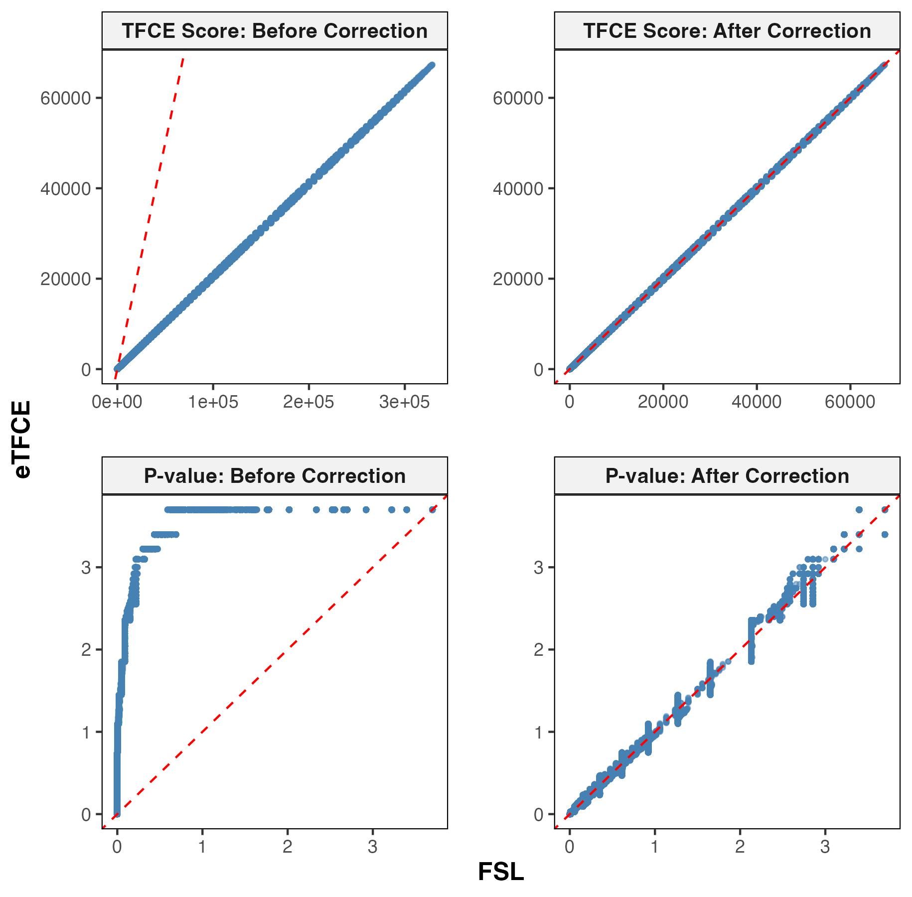
Figure 2 presents the comparison between eTFCE and FSL’s default TFCE implementation using this auditory dataset. The upper panel shows the voxel-wise TFCE scores before (left) and after (right) scaling error correction in FSL. The two methods differ proportionally before correction, while after correction, their TFCE scores closely align. The lower panel compares the FWER-corrected $p$-values for each voxel derived from TFCE, which incorporate spatial cluster information. Before correction (left panel), eTFCE consistently yields smaller $p$-values (uniformly more sensitive) than the uncorrected FSL implementation, as evidenced by all points lying on or above the identity line in the scatter plot. The systematic difference in the FSL implementation arises because, when true signal is present, the maximum voxel height $h_{\max}$ or the discrete step size $\Delta\tau$ in Equation (2) is generally larger in the original data than in the permuted data. This overestimation inflates the permutation null distribution, leading to overly conservative $p$-values for FSL. eTFCE does not suffer from this scaling bias. When the approximate results from FSL are corrected, the resulting $p$-values closely match those from the exact eTFCE method, as shown by the points distributed closely along the identity line (right panel). The disagreement in significance between the eTFCE results and the corrected FSL results is minimal, with only $0.14\%$ of voxels are significant under eTFCE but not under corrected FSL, and $0.01\%$ show the opposite pattern.

Figure 2: Comparison of eTFCE and FSL’s default TFCE on auditory data. Panels show results before (left) and after (right) scaling error correction. The TFCE scores are displayed in the top row, and the log-transformed FWER-corrected $p$-values ($-\log_{10}(p)$) are shown in the bottom row, derived from $5000$ sign-flipping randomizations. The red dashed lines correspond to the identity line.

4.3 Generalization across HCP Task Contrasts

Data

To extend the evaluation to different activation patterns (Noble2020), we also analyze six cognitive task contrasts, derived from the Human Connectome Project (HCP; Barch2013; VanEssen2013):

• Emotional processing: faces vs shapes,

• Incentive processing (gambling): punish vs reward,

• Language processing (story): math vs story,

• Relational processing: matching vs relational,

• Social cognition: theory of mind (ToM) vs random,

• N-back Working memory: 2-back vs 1-back.

Data from $80$ independent subjects was extracted from the HCP S1200 data release, with minimal preprocessing pipelines applied as described by Glasser2013. After preprocessing and first-level modeling (Barch2013), the task-specific contrast maps were analyzed at the group level.

Results

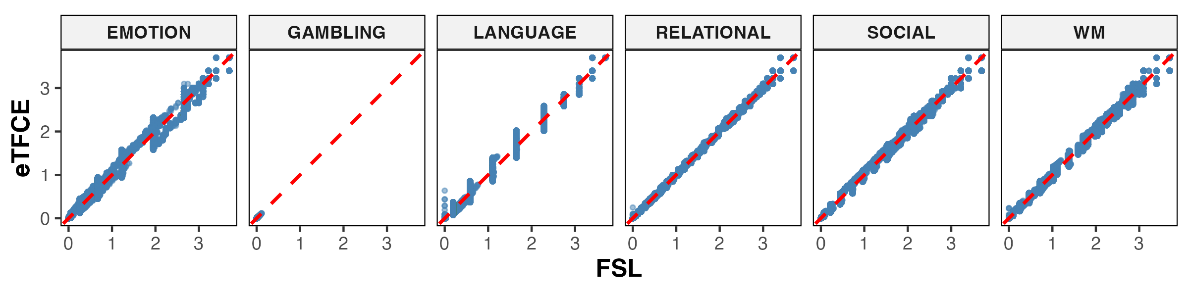
Figure 3 illustrates the resulting log-transformed, voxel-wise TFCE-based FWER-corrected $p$-value comparisons between eTFCE and FSL’s default implementation for the six HCP task contrasts. The upper panel shows the comparison between eTFCE and FSL before correcting the scaling error, while the lower panel shows the comparison after correction. Before correction (see Figure 3a), FSL is typically more conservative (yielding larger $p$-values) except for the Gambling contrast, where both methods consistently return very large $p$-values (close to $1$), thus indicating non-significant results. For the other five contrasts, FSL’s current default TFCE implementation consistently produces more conservative results than eTFCE. After correction (see Figure 3b), $p$-values from the two methods closely align, with over $99.67\%$ agreement in total. The minimal discrepancies could be attributed to the fact that eTFCE is an exact approach while FSL uses an approximate implementation.

(a) Comparison before scaling error correction for FSL.

(b) Comparison after scaling error correction for FSL.

Figure 3: Comparison of eTFCE and FSL’s default TFCE for $6$ cognitive task contrasts from the Human Connectome Project. The log-transformed FWER-corrected $p$-values ($-\log_{10}(p)$, based on $5000$ randomizations) are shown. (a) Results before applying scaling error correction to FSL’s TFCE. (b) Results after applying scaling error correction to FSL’s TFCE, which ensures a fair comparison with eTFCE. The red dashed lines indicate the identity line, and the six contrasts are: Emotional (faces vs shapes), Gambling (punish vs reward), Language (math vs story), Relational (matching vs relational), Social (ToM vs random), and WM (2-back vs 1-back).

4.4 Computational Efficiency

In addition to statistical performance, we compare the computational efficiency of eTFCE and FSL’s default TFCE on the auditory task and the six HCP task contrasts (see Table 1). We measure the running time required to compute the whole-brain TFCE map using the statistic map from each randomization, and report the average time per randomization across $5000$ sign flips.

A key algorithmic advantage contributing to the computational efficiency of eTFCE is its integrated design. Unlike FSL, eTFCE pre-constructs a disjoint-set forest from the statistic map only once. This data structure allows simultaneous computation of TFCE and cluster-related statistics (e.g., cluster extent and cluster mass) within the same resampling loop, at negligible additional cost. Consequently, our implementation requires only about $50\%$ of the average running time of FSL’s approximate TFCE.

This speed gain not only supports more accurate statistical inference but also makes robust nonparametric analysis more computationally accessible. Moreover, the integrated framework provides both TFCE maps and conventional cluster-level statistics from a single run. By enabling direct comparison across inference strategies within the same analysis, this framework provides improved effectiveness and efficiency relative to the standard TFCE implementation.

Table 1: Average running time (seconds) for whole-brain analysis over $5000$ randomizations: comparison between eTFCE (with disjoint-set forest pre-calculation) and FSL’s default TFCE implementation.

	eTFCE			FSL
Contrast	Forest Construction	TFCE	Extent & Mass1,2	TFCE	Extent1
Auditory	$0.574$	$0.017$	$0.002$	$1.172$	$0.133$
Emotion	$0.231$	$0.006$	$0.001$	$0.515$	$0.131$
Gambling	$0.239$	$0.006$	$0.001$	$0.545$	$0.135$
Language	$0.240$	$0.006$	$0.001$	$0.536$	$0.135$
Relational	$0.237$	$0.006$	$0.001$	$0.535$	$0.132$
Social	$0.243$	$0.007$	$0.001$	$0.553$	$0.139$
Working Memory	$0.230$	$0.006$	$0.001$	$0.521$	$0.131$

• ¹Supra-threshold clusters are generated using a CDT of $h\geq 3.1$.

• ²The reported time includes the combined computation of both cluster extent and cluster mass.

4.5 Integrated TFCE and CEI Inference

To demonstrate the practical effectiveness and adaptability of eTFCE’s computational framework, we apply it to the previously described auditory and HCP working memory contrasts, which exhibit distinct activation patterns (Noble2020). Rather than treating TFCE and cluster-extent inference (CEI) as alternative error control procedures, we employ their complementary sensitivities to characterize task-evoked spatial activation patterns.

For the auditory task (see Figure 4a), the primary temporal clusters are bilaterally symmetric and consistently detected by both methods. Most TFCE-specific significant voxels are located at the boundary of, or adjacent to, the clusters jointly identified by TFCE and CEI. In contrast, CEI uniquely detects additional spatially distinct non-temporal (frontal) clusters that contain few or no TFCE-significant voxels (see clusters indicated by black arrows). This pattern aligns with the focal, high-intensity activation characteristic of auditory processing. CEI captures additional frontal clusters despite relatively low intensity, while TFCE mainly enhances the core temporal regions. The partial overlap between methods suggests a pattern characterized by focal peaks embedded within broader regions of moderate activation.

For the working memory task (see Figure 4b), a distinct pattern is observed. Multiple bilateral clusters distributed across cortical and subcortical regions are identified. All CEI-significant clusters are also detected by TFCE, but TFCE reveals additional subcortical activation in caudate nuclei, thalamus, and brainstem (see areas indicated by black arrows), which is not detected by CEI, and no CEI-specific clusters are observed. This dissociation reflects the distributed, moderate-intensity nature of working memory activation. TFCE is more sensitive to spatially distributed weaker activation, while CEI requires more focal, concentrated activation.

These two examples demonstrate how eTFCE’s integrated inference provides complementary insights into the spatial organization of task-evoked activation. In the auditory task, partial overlap between CEI and TFCE reveals focal peaks with peripheral voxels and CEI-unique clusters, indicating heterogeneous spatial distribution. In the working memory task, extensive bilateral activation shows CEI-detected clusters nested within the broader TFCE map that additionally identifies subcortical regions. These findings highlight that different inference procedures reveal complementary sensitivities to the spatial organization of the underlying signal. Jointly considering them captures task-dependent patterns that would remain incomplete if only a single method is applied.

(a) Auditory: Eight CEI-significant clusters (blue shading, cluster-level FWER $p\leq 0.05$), overlaid on voxels surviving TFCE-based FWER correction (eTFCE, $p\leq 0.05$), colored by $-\log_{10}(p)$.

(b) HCP Working Memory: Six CEI-significant clusters (blue shading, cluster-level FWER $p\leq 0.05$), overlaid on voxels surviving TFCE-based FWER correction (eTFCE, $p\leq 0.05$), colored by $-\log_{10}(p)$.

Figure 4: Example visualization of integrated inference on two task contrasts with distinct spatial activation profiles. (a) Auditory discrimination task (vocal $>$ non-vocal), where CEI identifies focal, high-intensity activation as well as additional spatially distinct clusters (see black arrows), while most TFCE-specific voxels are distributed along the boundaries of, or adjacent to, shared clusters. (b) HCP working memory task (2-back $>$ 1-back), where multiple bilaterally symmetric clusters distributed across regions are detected by both methods. All CEI-significant clusters are also identified by TFCE, which further reveals additional subcortical activation (see black arrows).

5 Conclusion and Discussion

In summary, we have developed eTFCE by formulating an exact TFCE computation procedure and integrating an efficient cluster retrieval algorithm. Conventional methods often rely on approximations and tolerate numerical errors to achieve faster computation. In contrast, our data-adaptive implementation avoids such approximations and corrects the scaling errors present in the default TFCE implementation in FSL (version 6.0.7.19 and earlier). As a result, the novel eTFCE approach yields mathematically exact results while reducing computation time by approximately $50\%$. Achieving similar numerical accuracy with FSL’s TFCE would require a substantial reduction in the discretization step size, which could incur a significant computational cost that quickly becomes impractical for large-scale datasets.

More importantly, the integrated design of eTFCE enables multiple inference strategies (currently including TFCE, cluster extent, and cluster mass) to be computed within a single nonparametric run with little additional computation time. Without such integration, each method would require rerunning the entire analysis, which quickly becomes computationally prohibitive in large-scale neuroimaging studies. This unified computation facilitates systematic comparisons across inferential statistics, enabling more comprehensive interpretation of neuroimaging findings and revealing spatial patterns that are robust, complementary, and more informative when combining multiple inferential frameworks.

In addition to its immediate practical benefits, the eTFCE framework is also designed to be extensible. Although our empirical evaluation focuses on standard TFCE, the proposed formulation can be readily generalized to other TFCE variants. Moreover, the generalized formulation introduced in Section 3.4 suggests that the underlying computational strategy of eTFCE may extend to a broader family of cluster-based statistics that share similar structural properties.

Together, these features establish eTFCE as a flexible and extensible framework for nonparametric inference in neuroimaging, enabling systematic and computationally efficient comparisons across a wide family of cluster-based statistical methods within a unified implementation.

6 Acknowledgments

This work was supported by the London Mathematical Society Scheme 4: Research in Pairs grant (Ref. 42438 to X.C.).