Improved Grid-Based Simulation of Coulombic Dynamics

Abstract

Accurate time-dependent quantum dynamics of Coulombic systems on grid-based representations remains computationally demanding due to the singularity of the Coulomb potential, which necessitates extremely fine spatial grids to mitigate discretisation errors. We propose two complementary correction schemes that, under identical resource budgets, consistently outperform the uncorrected counterparts. The first scheme modifies the potential operator to incorporate grid-basis structure into its representation, while the second introduces a corrected initial wavefunction inspired by analytical solutions of softened Coulomb potentials. Applied to hydrogenic systems, these corrections deliver improved energy accuracy and time fidelity across long evolutions. Beyond classical simulations, the proposed framework aligns naturally with quantum computing architectures, where the corrected operators and states can be encoded through truncated Walsh and Fourier series expansions. A resource analysis for the representative 2D hydrogen system yields a circuit depth of $1.5\times 10^{8}$ gates over 6,000 Trotter steps. This study thus establishes practical strategies toward high-accuracy Coulombic dynamics on both classical and emerging quantum platforms.

I Introduction

Studying the quantum behaviour of Coulombic systems through direct simulation of the full wavefunction dynamics without invoking the Born–Oppenheimer approximation is at once the most conceptually simple approach, and yet extremely challenging to realise. While such simulations can provide detailed insight into electron-molecule scattering, absorption cross-sections, Auger decay and other fundamental processes in light-matter interaction and chemical reactivity, the complexity of the simulation grows exponentially with the number of particles and with the fidelity of the wavefunction representation, which presents severe challenges to the application of the approach.

A wide range of simulation techniques for Coulombic systems on classical computers have been developed and studied in depth over the years Gan et al. (2025); Schrader et al. (2024); Nys et al. (2024); Niklasson (2021); Rowan et al. (2020); Schütt et al. (2019); Füsti-Molnár and Pulay (2002). Researchers have sought to design reduced-cost strategies that combine compact wavefunction representations with practical time evolution protocols. Grid‐based approaches Schäfer et al. (2024); Li et al. (2024); Sereda et al. (2024); Silaev et al. (2023); Peng and Starace (2006); Gordon et al. (2006); Kawata and Kono (1999), such as finite difference or discrete variable representations, directly discretise the spatial domain, but limitations in the grid density introduce sizeable errors arising from poor resolution of near the singularities of electron-nucleus Coulomb interaction. Spectral methods that employ tailored orthogonal polynomial bases Dong et al. (2022); King et al. (2018); Zhao et al. (2023) can more accurately capture bound state features; however, they introduce artificial boundary conditions that distort continuum states. Path Integral techniques Dornheim et al. (2023); Schoof et al. (2011); Bonitz et al. (2003) use imaginary‐time propagation to handle singular potentials, but this comes at the cost of resolving real-time dynamics. Quantum Trajectory theory Svensson et al. (2023); Oriols (2007); Popruzhenko et al. (2008) evolves wavepackets in time via stochastic averaging, but fails to resolve multi-body quantum correlations.

The exponential growth of the complexity of the Hilbert space with system size forces a compromise in accuracy when using classical approaches. Quantum computing offers a paradigm shift for overcoming this limitation. This is due to a quantum computer’s capacity to encode an exponentially large Hilbert space with using linear number of qubits, and to leverage the inherent quantum superposition, entanglement and interference in the simulated dynamics Brown et al. (2010); Bauer et al. (2023); Temme et al. (2011). Specifically, for grid-based methods, the computational basis states of a quantum computer encode wavefunctions in discrete real-space as:

$$\begin{split}\underbrace{\sum^{2^{n}-1}_{j=0}c_{j}\ket{x_{j}}}_{\text{pixels in grid-based space}}=\underbrace{\sum^{2^{n}-1}_{j=0}c_{j}\ket{j}}_{\text{amplitudes in quantum computer}},\end{split}$$ (1)

with the number of stored amplitudes growing exponentially with the total qubit count $n$. The intrinsic interference between quantum amplitudes enables quantum computers to achieve exponential speed-ups over classical counterparts in simulating quantum dynamics Childs and van Dam (2010); Lloyd (1996).

Among various numerical methods for time-evolution, the grid-based Split Operator Fourier Transform (SO-FT) Mocken and Keitel (2008); Hermann and Fleck (1988); Kosloff (1988) stands out for its simplicity and its ability to exploit the diagonal dominance of kinetic and potential operators in momentum and real space, respectively. By decomposing the time evolution into alternating kinetic and potential updates, SO-FT achieves impressive performance across many scenarios. It exploits the Fourier Transform to switch between complementary spaces, leading to high efficiency when targeting time-dependent dynamics or spectroscopic properties at modest scales.

The SO-QFT approach represents a natural evolution of SO-FT towards the quantum platforms Chan et al. (2023); Childs et al. (2022); Kivlichan et al. (2020); Kassal et al. (2008); Zalka (1998), with the use of transformative Quantum Fourier Transform (QFT) Shor (1994); Cleve et al. (1998); Coppersmith (2002); Nielsen and Chuang (2010). At its core, the SO-QFT technique retains the well-established procedure of operator splitting to separately treat kinetic and potential contributions, allowing for sequential application in their respective spaces. Consequently, this methodology benefits from mitigating the numerical difficulties associated with the non-locality of kinetic operators in the real space. By replacing the classical Fourier transform component by the exponentially faster QFT, the SO-QFT framework stands as a promising candidate for future applications on quantum computers.

Notwithstanding the exponential compression of a $N^{d}$ direct-product grid of $N$-points each of $d$ dimensions onto $d\log_{2}N$ qubits, large values of $N$ are still required to simulate Coulombic systems due to the necessity to properly resolve the Coulomb singularities. Using too low resolution introduces discretisation artifacts in the simulated dynamics. In this paper we examine the discretisation error for simple model systems and propose two strategeies for suppressing discretisation artifacts. These efforts are designed to address the systematic inaccuracies caused by oversimplifying Coulomb-related terms in grid-based representations. Our study not only improves classical simulation fidelity, but also proposes gate-efficient mappings of the correction schemes essential for adaptation to fault-tolerant quantum hardware.

This paper is organized as follows. Section II details the foundational framework underlying our approach. Section III introduces the correction schemes employed to better accommodate Coulombic dynamics. Section IV presents classical emulation results to illustrate the efficacy of these corrections. Section V outlines the corresponding quantum circuit architectures, along with an analysis of their quantum resource demands.

II Foundational Framework

We begin by detailing the basic theoretical framework of our approach. This includes the spatial-grid scheme for quantum state representation, the systems studied in this work, the SO-QFT method for time evolution, and the extraction of time-dependent observables.

II.1 Grid-Based State Representation

In both classical and quantum computational frameworks, grid-based representations frequently utilise plane wave basis functions due to their completeness, orthogonality, and compatibility with periodic boundary conditions. Specifically, we consider a truncated momentum basis of finite $2\rho$ states, $|k\rangle$, each corresponding to a plane wave function:

$$\phi_{k}(x)=L^{-\frac{1}{2}}e^{i\frac{2\pi x}{L}k},$$

with $k\in{-\rho,\dotsc,\rho-1}$. Here $L$ represents the length of the position domain, which is chosen to ensure negligible boundary amplitude during the time evolution. Upon application of the inverse Fourier transform, these momentum-space basis states are mapped to a set of dual states $|j\rangle$:

$$\phi_{j}(x)=\frac{1}{\sqrt{2\rho}}\sum_{k=-\rho}^{\rho-1}e^{-i\frac{2\pi k}{L}x_{j}}\phi_{k}(x),$$

where each ‘pixel function’ $\phi_{j}(x)$ in the position space is sharply peaked at the grid position $x_{j}=\frac{jL}{2\rho}$. As $2\rho\to\infty$, these pixel functions converge to exact Dirac delta functions: $\phi_{j}(x)\to\delta(x-x_{j})$ Chan et al. (2023).

In this work, we study quantum dynamics under the Coulomb potential using this grid-based discretisation. Each position grid point is associated with a single amplitude of the wavefunction, assuming that the pixel function is negligible away from its central peak (i.e. $\phi_{j}(x)=0$ at all $x_{m\neq j}$ points and only peaked at $x_{j}$). This amounts to discretisation errors, wherein the spatially continuous potential and wavefunction are represented by their values on discrete grid points. As either attractive or repulsive Coulomb potential is centered at the origin, the singularity at $x=0$ poses numerical difficulties. To prevent divergence, the grid is defined to avoid including this point explicitly. This exclusion, along with the sparse nature of grid-based discretisation, introduces artifacts in ground-state energies and time evolution fidelity. Denser grids mitigate this issue but at the expense of increased computational resources. In this work, we propose correction schemes that recover high fidelity with moderate grid sizes.

II.2 Model Systems

Our analyses focus on two characteristic simple Coulombic systems, which are small enough to allow simulations with very dense grids and long-time evoluions with short time steps. Our model systems are a 2D hydrogen system, and the 2-electron quantum ring. The Hamiltonian for 2D hydrogen Yang et al. (1991) is

$$H_{\text{hydrogen}}=\underbrace{-\frac{1}{2}\frac{\partial^{2}}{\partial x^{2}}-\frac{1}{2}\frac{\partial^{2}}{\partial y^{2}}\ }_{K}+\underbrace{\frac{1}{\mathbf{r}}}_{V}\ ,$$ (2)

where the nucleus is treated as a fixed Coulombic center. The analytic solution for the ground state is known

$$\Psi_{\text{hydrogen}}=Ce^{-2\mathbf{r}},$$ (3)

and the ground state energy is -2 a.u.. Here $\mathbf{r}=\sqrt{x^{2}+y^{2}}$ and $C$ incorporates all constant factors in the wavefunction. We define a square simulation box of length 10 a.u centred at the nucleus. The number of grid points in each of the two spatial dimensions determines the resolution of the electron’s position, with higher grid density yielding finer spatial details.

The Hamiltonian for the 2-electron quantum ring is

$$H_{2e}=\underbrace{-\frac{1}{R^{2}}\frac{\partial^{2}}{\partial\omega^{2}}\ }_{K}+\underbrace{\frac{1}{\mathbf{u}}}_{V}\ ,$$ (4)

where the radius $R=1/2$ and $\mathbf{u}=R\sqrt{2-2\cos{\omega}}$, where $\omega$ is the angular separation of electrons on the ring. The analytic ground state is

$$\Psi_{\text{2e}}=\mathbf{u}(1+\frac{\mathbf{u}}{2R})^{1/2},$$ (5)

and has an energy of 2.25 a.u. Loos and Gill (2012)

$$H_{2e}=\underbrace{-\frac{1}{R^{2}}\frac{\partial^{2}}{\partial\omega^{2}}\ }_{K}+\underbrace{\frac{1}{\mathbf{u}}}_{V}\ ,$$ (6)

The angle $\omega$ is called the intracule angle coordinate and spans $[0,2\pi]$. This angular variable is discretised to control the spatial resolution. Atomic units are used for all simulations.

II.3 Time Propagation

In the SO-QFT method, the time evolution is decomposed into alternating kinetic and potential operator actions via the symmetric Trotter-Suzuki formula, from which errors occur due to the non-commutativity between partitioned Hamiltonian terms. Adopting the second order form Suzuki (1976, 1985); Hatano and Suzuki (2005) bounds this error scaling within $\mathcal{O}(dt^{3})$:

$$e^{-iHdt}=e^{-iVdt/2}e^{-iKdt}e^{-iVdt/2}+\mathcal{O}(dt^{3}),$$ (7)

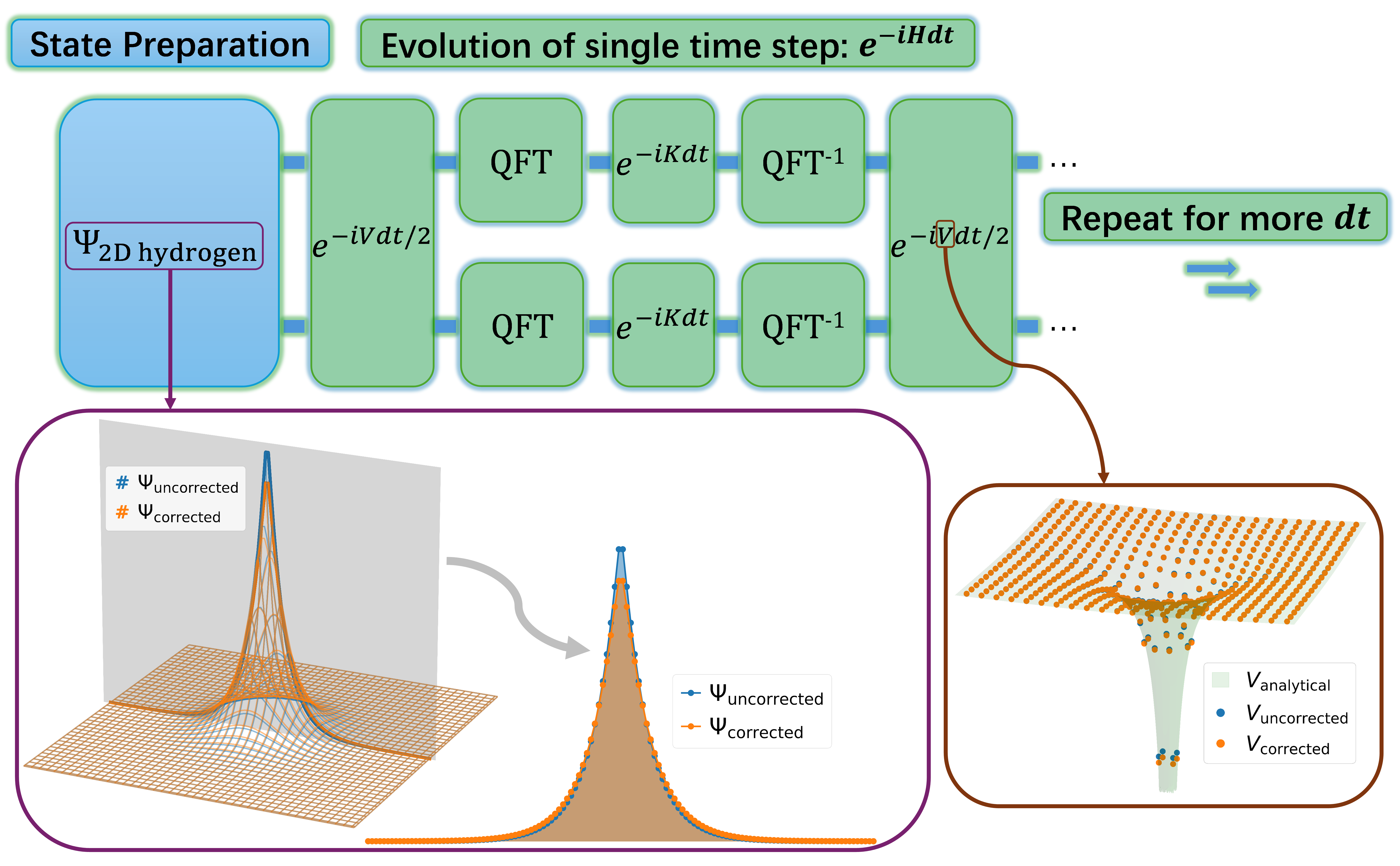
where $dt$ denotes the discretisation interval between adjacent time steps. This symmetric workflow proceeds through (i) a half-step potential operator $e^{-iVdt/2}$ in the position space, (ii) a full-step kinetic operator $e^{-iKdt}$ executed via QFT-mediated momentum-space propagation, and (iii) a concluding half-step potential update $e^{-iVdt/2}$. All simulations in this work are conducted under a sufficiently high time resolution, e.g., 30,000 steps ($dt=0.0002$ a.u.) for the 2-electron quantum ring and 6,000 steps ($dt=0.001$ a.u.) for 2D hydrogen over a total duration of 6 a.u., to minimise the impact of time discretisation and enabling a focused evaluation of spatial resolution effects.

Conversions between position and momentum spaces are typically performed using Fourier Transform. On classical platforms, this process is commonly realised via the fast Fourier Transform (FFT), which scales as $\mathcal{O}(n2^{n})$ for a vector of size $N=2^{n}$. In contrast, the QFT provides an exponentially more efficient mechanism, requiring only $\mathcal{O}(n^{2})$ gates for $n$-qubit systems.

II.4 Extraction of Observables

Within the SO-QFT framework, the total evolution time is discretised into finite steps. We monitor two key observables during time evolution: the dynamic ground-state energy and the evolution fidelity. Both are derived from the time-dependent autocorrelation function,

$$A(t)=\langle\Psi(t)|\Psi(0)\rangle=e^{iE_{\text{dynamic}}t},$$ (8)

which is the inner product of the time-evolved state at time $t$ with the initial state at $t=0$ Nauenberg (1990). The cosine periodicity of its real component, $\cos{(E_{\text{dynamic}}t)}$, enables retrieval of this time-averaged numerical energy, $E_{\text{dynamic}}$, which reflects the energy scale governing long-time dynamics and serves as a robust indicator for algorithmic accuracy. Under a perfect simulation, $E_{\text{dynamic}}$ is expected to be the exact analytical ground-state energy. Fidelity, on the other hand, is evaluated by the absolute value of the autocorrelation function. For systems initiated in eigenstates of the Hamiltonian, this modulus should ideally remain unity throughout time evolution:

$$\lvert A(t)\rvert=\lvert\langle\Psi_{n}(t)|\Psi_{n}(0)\rangle\rvert=1.$$

Any deviation indicates fidelity loss and thus provides a quantitative measure of temporal coherence in the simulated dynamics.

III Correction Schemes

In conventional grid-based simulations, potentials are applied pointwise on a discretised spatial grid, implicitly assuming each basis function as a Dirac delta function. While a small number of simulation grid points suffice for smooth fields e.g. quadratic potentials, the inability to resolve the singularities near their origins introduce errors when representing dynamics with e.g. the Coulomb interaction, particularly under a limited grid resolution. The immediate assumption that a higher spatial resolution via an increased grid density leads to improved accuracy is widely held. Yet, this direct scaling of resolution, while conceptually straightforward, exhibits intensive computational burden for large systems. This trade-off becomes problematic in scenarios necessitating prolonged time propagation, rendering it less than ideal for practical applications.

To address this, we propose a correction scheme in which the Coulomb potential is re-evaluated by computing the expectation value of the original Coulomb potential within the actual pixel function $\phi_{j}(x)$. Specifically, we define a corrected potential

$$\begin{split}V_{\text{corrected}}&=\langle\phi_{i}(x)|V|\phi_{k}(x)\rangle\text{ (in 1D)},\\ &=\langle\phi_{i}(x)\phi_{j}(y)|V|\phi_{l}(y)\phi_{k}(x)\rangle\text{ (in 2D)},\\ &=\cdots\end{split}$$ (9)

which accounts for the spatial extent and shape of the localized pixel functions and more accurately reflects the singular potential’s influence over the local region. An independent auxiliary grid, $N_{\text{correction}}$ per dimension, is used to evaluate these matrix elements. For computational convenience of this work, we have limited our consideration to contributions arising solely from the diagonal elements, where $i=k$ and $j=l$.

The new set of potential values, $V_{\text{corrected}}$, is used during simulation in place of the naive point-sampling potential. Although the simulation itself still runs on the original coarse grid $N_{\text{simulation}}$, using a denser auxiliary $N_{\text{correction}}$ for the numerical calculation of $V_{\text{corrected}}$ yields significant performance improvements in both the ground-state energy integrity throughout time-dependent dynamics and the evolution fidelity as a function of time (see Section IV.1). This correction leverages higher-resolution information in the preprocessing stage while keeping the computational complexity of the main simulation unchanged.

Another challenge in grid-based simulations involving Coulomb systems lies in initial state determination, which would typically be the ground state of the system in the absence of a perturbing interaction. In low-resolution grids, the ground state of the low-resolution Hamiltonian differs from the exact eigenfunction and we must decide whether to initialise with a close approximation to the eigenstate of the Hamiltonian we evolve with, or a close approximation to the eigenstate of the analytic solution. To obtain consistent and stable dynamics that converges systematically to the analytic behaviour with increasing resolution, one should choose the former and prepare an initial eigenstate of the low-resolution Hamiltonian. The low-resolution Coulombic interaction essentially replaces the sharp singularity with a softened Coulombic interaction. Inspired by prior analytical solutions of hydrogenic systems derived from softened Coulomb potentials Li (2021), we propose to use

$$\begin{split}&\Psi_{\text{corrected}}=C\mathbf{r}^{\frac{Z}{\alpha}-b}e^{-\alpha\mathbf{r}},\end{split}$$ (10)

as a corrected wavefunction to reduce the numerical mismatch between the initial state and the grid-based Hamiltonian. Here $b=0,-\frac{1}{2},-1$ for 1D, 2D and 3D hydrogenic models, and $\alpha=\sqrt{-2E_{\text{dynamic}}}$ . In this formulation, all constant coefficients are absorbed into the prefactor $C$. Since $E_{\text{dynamic}}$ varies with the grid density employed in the numerical simulation, the parameter $\alpha$ must be uniquely calculated for each specific grid density. Thus, by running a preliminary trial simulation at the chosen spatial resolution, one can determine $E_{\text{dynamic}}$, calculate the corresponding $\alpha$, and subsequently derive the corrected wavefunction $\Psi_{\text{corrected}}$.

Our results (see Section IV.2) on the 2D hydrogen system confirm that initializing the simulation with this corrected wavefunction yields extremely high time fidelity, validating its effectiveness. As $\Psi_{\text{corrected}}$ more closely approximates the true physical state in grid-based space, this correction scheme enables stable time-dependent studies without requiring prohibitively dense grid resolutions.

While demonstrated here for hydrogenic systems, the strategy of modifying initial wavefunctions holds potential for broader applications beyond the current context. For other Coulombic systems where analytical eigenfunctions of analogous softened potential approximations are available, similar corrections can be deduced. For more complex molecular systems a succussfull scheme may involve using corrected atomic orbital expansions as good initial states. This offers a systematic means to enhance simulation reliability and without resorting to impractical grid refinements, thus broadening the applicability of grid-based quantum dynamics methods.

IV Performance of Correction Schemes

We first assess the general characteristics of the SO-QFT scheme in systems featuring singular Coulombic potentials – which we will reference as the uncorrected benchmark. As a representative case, we herein present results of the 1D two-electron quantum ring. Figure 1 illustrates that, in the absence of correction, the numerical ground-state energies extracted from $\operatorname{\mathbb{R}e}\{A(t)\}$ gradually converge to the known analytical value and the $|A(t)|$ curves reflecting time fidelity present deviates less from unity, as the spatial resolution increases (i.e., the number of grid points $N_{\text{simulation}}$ increases within the fixed angular domain $[0,2\pi]$). As expected, increasing grid density improves energy estimate and time fidelity, but incurs a steep computational cost in terms of memory and gate complexity, posing a practical limitation on such a brute-force approach. This motivates the use of correction schemes that can suppress errors even for coarse grid settings.

Figure 1: Absolute value and real part of autocorrelation functions recorded from simulating the 2-electron quantum ring with different $N_{\text{simulation}}$. Analytical profiles are plotted with dashed linestyle.

We therefore evaluate the efficacy of our two correction schemes in improving overall simulation quality, still using two complementary indicators: The numerical ground-state energy $E_{\text{dynamic}}$ for algorithmic accuracy and the modulus of the autocorrelation for fidelity retention over time.

IV.1 Potential Operator Corrections

(a) Autocorrelation for the 2-electron quantum ring

(b) Autocorrelation for the 2D hydrogen

Figure 2: Absolute value and real part of autocorrelation functions recorded from simulations of (a) the 2-electron quantum ring and (b) the 2D hydrogen using $V_{\text{corrected}}$ computed from different $N_{\text{correction}}$. For both panels, $N_{\text{simulation}}$ is fixed at 128 per dimension. Analytical profiles and results from uncorrected runs are plotted with dashed and dotted linestyles, respectively.

Diagonal corrections on the potential operator decouple the grid density used for physical propagation from that used for numerical calculation of the basis-integrated $V_{\text{corrected}}$. We run simulations under $V_{\text{corrected}}$ with the same simulation grid size $N_{\text{simulation}}$ per dimension (as above) but vary the number of auxiliary correction grids $N_{\text{correction}}$, as shown in Figure 2.

Compared to uncorrected benchmarks, these numerical results confirm that simulations using $V_{\text{corrected}}$ display improved agreement with analytical energies and show enhanced time fidelity for both the 1D two-electron quantum ring and the 2D hydrogen systems. This behaviour is rationalized by the fact that the corrected potential captures more of the singular feature of the Coulomb interaction that would otherwise be missed in such low-resolution simulations.

In addition, as the density of the quadrature grid $N_{\text{correction}}$ increases, both the extracted $E_{\text{dynamic}}$ and $|A(t)|$ exhibit improvements. By resolving more of the pixel function’s structure in the correction step, we achieve better modeling of the potential landscape. Technically, we only need to calculate $V_{\text{corrected}}$ once and the computational cost involved will not be escalated during long-time propagation.

As each entry in $V_{\text{corrected}}$ is computed by integrating over $N_{\text{correction}}^{d}$ grid points for $d$-dimensional systems, the major limitation lies in the exponentially increasing cost with system dimensionality. To make this step more scalable, we explore a piecewise non-uniform grid that concentrates points near the origin (where singularities occur), and allocates coarser spacing elsewhere.

As seen in Table 1, the energy values simulated using the non-uniform grid are close to those using much more uniform grids, provided the central resolution is comparable. The key insight is that the dominant contributions to the potential correction arise near the singularity, justifying the use of non-uniform strategy for higher-dimensional calculations to avoid the overhead of uniformly dense grids.

Central Spacing	$N_{\text{correction}}$ within $[-5,5]$		$E_{\text{dynamic}}$
0.002	Non-Uniform	1800	-1.775
	Uniform	5000	-1.774
0.001	Non-Uniform	2800	-1.777
	Uniform	10000	-1.776

Table 1: Simulated $E_{\text{dynamic}}$ of the 2D hydrogen system using uniform and non-uniform grid allocations in $V_{\text{corrected}}$ calculation. In the non-uniform cases, $N_{\text{correction}}=$ 1800 and 2800 represent that 1000 and 2000 grid points are assigned within the central region, $[-1,1]$ a.u., respectively, while the outer tails ($[1,5]$ a.u. and $[-5,-1]$ a.u.) are allocated with 800 grid points.

IV.2 Initial Wavefunction Corrections

Here we evaluate the impact of wavefunction correction on time propagation fidelity. In Figure 3, simulations initialized with corrected wavefunctions demonstrate near-perfect time fidelity. Across spatial grids of varying resolution examined ($N_{\text{simulation}}=64,128,256$), the corrected cases keep tightly aligned with the ideal $|A(t)|=1$ benchmark, in stark contrast to the visible deviations seen in the uncorrected runs. This indicates that the correction effectively recovers eigenstate-like stability and the benefit extends to various $N_{\text{simulation}}$, confirming the robustness of utilising corrected initial states for maintaining high time fidelity even in coarse grids.

Figure 3: Absolute value of autocorrelation functions recorded from 2D hydrogen simulations initialized with uncorrected and corrected wavefunctions across different $N_{\text{simulation}}$.

While the potential correction optimises $E_{\text{dynamic}}$ and the wavefunction correction preserves time fidelity, we have examined that they together produce synergistic improvements. In simulations of the 2D hydrogen that simultaneously applies both corrections, the absolute autocorrelation remains ideal behaviour throughout and the numerical energy $E_{\text{dynamic}}$ fully exhibit the benefit of the corrected potential. This dual-correction strategy is particularly suited for systems where increasing $N_{\text{simulation}}$ is computationally expensive, as it enables better-quality simulations than uncorrected baselines when holding the grid density unchanged.

V Quantum Implementation of Corrected Coulombic System Dynamics

With the rapid progress in quantum computing, simulations of real-space Coulombic systems are expected to become significantly more tractable and efficient once practical quantum simulators are available Low et al. (2025). We therefore seek to investigate the efficient realisation of our algorithm on quantum computers. The key properties of interest in this work, $E_{\text{dynamic}}$ and time fidelity, are both derived from the time-dependent autocorrelation function. The extraction of this function maps directly to the measurement stage within the corresponding quantum algorithm.

Figure 4: Schematic circuit for measuring the real part of autocorrelation functions at a specific time step.

Figure 5: Schematic overview of essential components for simulating the 2D hydrogen system.

Quantum Phase Estimation (QPE) Aspuru-Guzik et al. (2005); Cruz et al. (2020); Svore et al. (2013) lies at the core of many quantum algorithms, enabling accurate measurement of eigenvalues for unitary operators. A simplified version of QPE is the Hadamard test Patel et al. (2025); Ding and Lin (2023), which requires only a single ancillary qubit and two Hadamard gates, as shown in Figure 4. In this setup, the system undergoes controlled time evolution up to a given time step, followed by measurement of the ancilla qubit. Repeated measurements yield the probabilities of observing $\ket{0}$ and $\ket{1}$, from which the real part of the autocorrelation at this time step is computed as

$$\operatorname{\mathbb{R}e}\{A(t)\}=P_{\ket{\text{ancilla}}}(0)-P_{\ket{\text{ancilla}}}(1).$$

Similarly, the imaginary part of the autocorrelation is obtained via

$$\operatorname{\mathbb{I}m}\{A(t)\}=P_{\ket{\text{ancilla}}}(1)-P_{\ket{\text{ancilla}}}(0),$$

by inserting an additional $\mathbf{S}$ gate before the final Hadamard gate.

The measurement count serves as one of the metrics when assessing quantum resources. This cost can be reduced by employing a sparser sampling strategy, i.e., measuring the ancilla at selected time points with wider intervals, provided the resulting autocorrelation remains sufficiently smooth to resolve the desired properties.

Another essential factor in resource evaluation is the circuit depth, which depends on the specific structure of the quantum circuits. In addition to autocorrelation measurements, the complete circuit also involves initial state preparation and time propagation stages. For these two stages, we have proposed and analysed two targeted correction schemes in previous sections, both of which are compatible with quantum architectures. In the remainder of this section, we focus on the 2D Hydrogen system as an illustrative example to detail the application of these correction schemes on realistic quantum hardware, along with an analysis of the associated gate depths and resource implications for constructing the circuit shown in Figure 5.

V.1 Preparation of Corrected Wavefunction

This section describes the quantum circuit construction for encoding the corrected wavefunction onto a register that represents a two-dimensional spatial space. We allocate $n=\log_{2}{N_{\text{simulation}}}$ qubits per spatial dimension to represent a 2D $N_{\text{simulation}}\times N_{\text{simulation}}$ grid. The resulting quantum register consists of two $n$-qubit sub-registers, initialized in the state $\ket{0}^{\otimes 2n}$. The goal is to transform this initial state into a superposition state that reflects the amplitudes of the corrected wavefunction, i.e.,

$$\sum^{2^{n}-1}_{j_{1}=0}\sum^{2^{n}-1}_{j_{2}=0}c_{j_{1}j_{2}}\ket{j_{1}}\otimes\ket{j_{2}},$$

where the coefficients $c_{j_{1}j_{2}}$ denote the discretised amplitudes. Each basis state $\ket{j_{1}}\otimes\ket{j_{2}}$ corresponds to a specific grid point within the 2D space.

One straightforward approach for preparing this quantum state is to treat the two spatial dimensions as a single index and load the $2^{2n}$ amplitudes directly onto a $2n$-qubit register. This can be implemented by a cascade of uniformly-controlled rotations Möttönen et al. (2004) requiring a gate count of $2^{2n+1}-3$, where only two-qubit $\mathbf{CNOT}$ gates and single-qubit $\mathbf{R_{y}}$ gates are used due to the real and non-negative nature of the amplitudes. For $n=\log_{2}{128}=7$, the total gate count is estimated to be 32,765.

To reduce the gate depth and improve efficiency, we alternatively adopt the Fourier Series Loader (FSL) method Moosa et al. (2023), which constructs the multidimensional quantum state from truncated Fourier series representations. Instead of loading all $2^{2n}$ amplitudes directly, only $2^{2l}$ Fourier coefficients with $l<n$ are used to approximate the full wavefunction.

Figure 6: Autocorrelation functions recorded from 2D hydrogen simulations initialized with corrected wavefunctions prepared by FSL method. $l$ represents the truncation level used in the state preparation. Benchmark data simulated from the exact corrected wavefunction ($n=7$) are displayed in dashed linestyle.

Figure 7: Circuit fragment corresponding to the $b=4$ partition group. The four remaining indices $\{12,15,10,9\}$ are arranged in gray-code order.

A truncated set of Fourier coefficients is first precomputed classically from the corrected wavefunction and used to initialize a compact quantum state onto a $2l$-qubit register. The loading circuit implements sequences of uniformly controlled rotations including alternating layers of $\mathbf{CNOT}$ gates interleaved with both $\mathbf{R_{y}}$ and $\mathbf{R_{z}}$ gates that result in total $2(2^{2l+1}-3)$ gates. The remaining $n-l$ qubits per dimension are then activated via entangling operations of $n-l$ $\mathbf{CNOT}$ gates, which effectively expands the state to the full $2n$-qubit register by zero-padding. Finally, an inverse QFT maps the encoded amplitudes to real-space. The total number of gates for this FSL procedure is denoted by $2^{2l+2}+n^{2}/2+2n-l-13/2$ (for odd $n$).

The choice of truncation level $l$ depends on the trade-off between simulation fidelity and gate complexity. For instance, by fixing $n=7$, we benchmark FSL-based initial states prepared from Qiskit Javadi-Abhari et al. (2024); Moosa et al. (2023) with varying $l$ values against the exact corrected wavefunction. Figure 6 shows that with $l=6$, the time-dependent autocorrelation remains fully consistent with the exact result. The corresponding gate count, 16,410, is nearly half of that required by full-amplitude loading. Further reduction to $l=5$ introduces minor deviations and undesirable oscillations in $A|(t)|$, but still fundamentally preserves the global stability of autocorrelation behaviours.

V.2 Implementation of Time Propagation

Simulating quantum dynamics on digital quantum hardware requires careful construction of the time evolution operator using gate-efficient techniques. In this section, we present the quantum implementation of time propagation under the Trotterized Hamiltonian. The full circuit is composed of three fundamental components: the kinetic evolution operator, the potential evolution operator, and the QFT that facilitates conversion between position and momentum spaces, as illustrated in Figure 5. Here the QFT and its inverse block are applied before and after the kinetic term, respectively, each introducing $n^{2}/2+n-1/2$ gates for odd $n$.

The kinetic evolution operator takes the form of an exponentiated quadratic polynomial in the momentum basis, which can be succinctly complied into successive controlled $\mathbf{U_{1}}$ gates Ollitrault et al. (2020). For the 2D hydrogen system, it factorizes along dimensions and can be applied in parallel across the respective $n$-qubit sub-registers:

$$e^{-iKdt}=e^{(\frac{-ip_{x}^{2}dt}{2})}e^{(\frac{-ip_{y}^{2}dt}{2})},$$

resulting in a gate count of $n^{2}$ per Trotter step.

We then turn to the potential evolution operator, $e^{-iV_{\text{corrected}}dt/2}$, which is implemented directly in the position basis. A compact and ancilla-free method for realising such diagonal unitary by Walsh-operator formalism has been proposed by Welch et al. (2014), which first maps the target unitary into a product of exponentials of Walsh Operators, and then reorder them to reduce repeated $\mathbf{CNOT}$ gates.

We begin with computing the Walsh–Hadamard coefficients $a_{j}$s via the Walsh-Hadamard Transform (WHT) of the discrete $F=-V_{\text{corrected}}dt$ (including $N_{\text{total}}=2^{2n}$ real values). The potential evolution operator $e^{iF}=e^{-iV_{\text{corrected}}dt}$ therefore maps to the quantum gate sequence

$$\prod_{j=0}^{N_{\text{total}}-1}e^{-ia_{j}\omega_{j}},$$

where $\omega_{j}$ is the Walsh operator indexed by the Paley order $j$.

These $j$ values are grouped by the most significant non-zero bit, $b$, of their binary representation $\ket{j}$. Within each such partition, the circuit implements alternating layers of $\mathbf{R_{z}}(2a_{j})_{[b]}$ and $\mathbf{CNOT}_{[b]}^{[c]}$ gates, with the subscript and superscript representing target and control qubits, respectively. Specifically, a $\mathbf{CNOT}_{[b]}^{[c]}$ gate is introduced only when the $c$th bit of the bitwise XOR between adjacent $\ket{j}$ is non-zero. Additional $\mathbf{CNOT}_{[b]}^{[c]}$ gates accounting for the XOR between the first and last $\ket{j}$ in each group are inserted at its beginning.

As shown in Welch et al. (2014), an optimal circuit construction with $2^{2n+1}-3$ gates is achieved by ordering the $N_{\text{total}}$ $\mathbf{R_{z}}(2a_{j})_{[b]}$ gates in Gray‑code sequence, which leaves just a single $\mathbf{CNOT}$ between successive $\ket{j}$ values. In practice, however, the number of non-trivial Walsh components is often much smaller than $N_{\text{total}}$, and discarding those $a_{j}$ near zero significantly simplifies the circuit while preserving autocorrelation behaviours.

For example, with $n=7$ qubits per sub-register, we find that retaining only the largest $N_{\text{approx}}=2^{12}$ coefficients (instead of the full $2^{14}$) still generates $E_{\text{dynamic}}$ and time fidelity indistinguishable from using the exhaustive series. Consequently, the number of $\mathbf{R_{z}}(2a_{j})$ gates reduces to $2^{12}=4096$. Arranging this truncated set of $2^{12}$ indices in Gray‑code order produces 8312 $\mathbf{CNOT}$ gates. Therefore, the total gate count for implementing $e^{-iV_{\text{corrected}}dt/2}$ is 12408. Figure 7 illustrates a representative fragment of the constructed circuit corresponding to the partition group of $b=4$, where only four $j$ values, $\{12,15,10,9\}$, survive the truncation.

Following the structure shown in Figure 5, the propagation of one single time step $dt$ includes the full‑step kinetic evolution, both half‑step potential evolutions, and double QFTs, which amounts to 24927 gates in total. For 6000 steps, the circuit depth scales linearly to $\sim 1.5\times 10^{8}$ gates.

VI Conclusions

The grid-based SO-FT method employed in this work has wide applicability in simulating time-propagated quantum dynamics. However, its accuracy degrades in the presence of Coulombic singularities, as the associated infinite value cannot be adequately represented using finite grids. While increasing grid density mitigates this error by more closely depicting the divergence, the exponential scaling of computational memory presents a major burden, especially for simulations with numerous Trotter steps. We therefore develop two correction schemes, one targeting Hamiltonian and the other focusing on wavefunction, to improve the robustness of Coulombic system simulations while maintaining the existing coarse grids.

The first correction reformulates the Coulomb potential by calculating its expectation value under the actual grid basis functions. This correction is pre-computed once and does not inflate costs during the time evolution. Our simulations in 1D electron-electron quantum ring and 2D nucleus-electron hydrogen systems validate the ability of the corrected potential to reduce bias in numerical energy and stabilize time fidelity. The second scheme concerns a wavefunction correction based on analytic solutions of soft Coulomb potentials. By incorporating additional polynomials and energy terms calibrated to specific grid resolution into the initial state, we create an initial state for 2D hydrogen that better represents the eigenstate of its grid-based Hamiltonian. Starting from this corrected wavefunction yields near-perfect time fidelity throughout the evolution window.

Although the corrections do not reproduce the exact singular behaviour, they consistently deliver smaller errors than the uncorrected forms. Because the associated deviation is systematic rather than stochastic, e.g., manifesting as quantifiable differences between corrected and analytical ground-state energies, it can be readily incorporated into analyses and practically subtracted as a correctible offset if necessary. Our correction schemes may offer tangible benefits when applied to more complex scenarios, such as simulations of multi-component systems involving hydrogen interacting with heavier atoms or under the influence of spatially varying external potentials (e.g., electric or magnetic). In such settings, small numerical inaccuracies can be amplified and distort long-range interactions. The outlined strategies help reduce cumulative numerical errors and facilitate improved stability, leading to more reliable predictions of system dynamics.

Extending the classical grid-based SO-FT method to its quantum analogue is straightforward, owing to the structural compatibility of grid-based representations with quantum registers and the inherent efficiency of QFT implementations. Within this framework, the correction schemes proposed in this work also adapt readily to quantum computing architectures. The corrected potential operator can be implemented using a truncated Walsh expansion, while the corrected wavefunction is prepared through a truncated Fourier series. By appropriately selecting truncation thresholds to preserve simulation accuracy, we estimate a circuit depth of $\sim 1.5\times 10^{8}$ gates for simulating a 2D hydrogen system with $n=7$ qubits per dimension over 6,000 Trotter steps.

Future optimisations will be directed toward broadening the scope and efficiency of these corrections. On the algorithmic side, incorporating off-diagonal contributions into the potential correction may improve accuracy by accounting for inter-basis overlaps that are currently neglected. Similarly, generalising the wavefunction correction to more Coulombic systems will expand its versatility. From a quantum computing perspective, these correction schemes are compelling for minimising error accumulation without demanding additional qubits, which is particularly advantageous in resource-constrained regimes. Embedding them into large-scale models could enable high-fidelity quantum simulations under realistic computational budgets.

VII Author Contributions

Xiaoning Feng conceived the project, developed the algorithm, performed the simulations, carried out the data analysis, and wrote the original draft of the manuscript. David P. Tew supervised the research and provided scientific guidance on the research design and interpretation of the results. Hans Hon Sang Chan provided supportive feedback through discussions.

VIII Conflicts of Interest

The authors declare that they have no competing interests.

References

- Gan et al. (2025) Z. Gan, X. Gao, J. Liang, and Z. Xu, Journal of Computational Physics 524, 113733 (2025).
- Schrader et al. (2024) S. E. Schrader, H. E. Kristiansen, T. B. Pedersen, and S. Kvaal, The Journal of Chemical Physics 161 (2024), 10.1063/5.0213576.
- Nys et al. (2024) J. Nys, G. Pescia, A. Sinibaldi, and G. Carleo, Nature Communications 15, 9404 (2024).
- Niklasson (2021) A. M. N. Niklasson, The Journal of Chemical Physics 154, 054101 (2021), https://pubs.aip.org/aip/jcp/article-pdf/doi/10.1063/5.0038190/14762701/054101_1_online.pdf .
- Rowan et al. (2020) K. Rowan, L. Schatzki, T. Zaklama, Y. Suzuki, K. Watanabe, and K. Varga, Physical Review E 101 (2020), 10.1103/physreve.101.023313.
- Schütt et al. (2019) K. T. Schütt, M. Gastegger, A. Tkatchenko, K.-R. Müller, and R. J. Maurer, Nature Communications 10, 5024 (2019).
- Füsti-Molnár and Pulay (2002) L. Füsti-Molnár and P. Pulay, The Journal of Chemical Physics 117, 7827 (2002), https://pubs.aip.org/aip/jcp/article-pdf/117/17/7827/19209750/7827_1_online.pdf .
- Schäfer et al. (2024) T. Schäfer, W. Z. Van Benschoten, J. J. Shepherd, and A. Grüneis, The Journal of Chemical Physics 160 (2024), 10.1063/5.0182729.
- Li et al. (2024) Y. Li, F. He, T. Sato, and K. L. Ishikawa, The Journal of Physical Chemistry A 128, 1523 (2024).
- Sereda et al. (2024) M. Sereda, T. Allen, N. C. Bradbury, K. Z. Ibrahim, and D. Neuhauser, Journal of Chemical Theory and Computation 20, 4196 (2024).
- Silaev et al. (2023) A. A. Silaev, A. A. Romanov, M. V. Silaeva, and N. V. Vvedenskii, Phys. Rev. A 108, 013118 (2023).
- Peng and Starace (2006) L.-Y. Peng and A. F. Starace, The Journal of Chemical Physics 125 (2006), 10.1063/1.2358351.
- Gordon et al. (2006) A. Gordon, C. Jirauschek, and F. X. Kärtner, Phys. Rev. A 73, 042505 (2006).
- Kawata and Kono (1999) I. Kawata and H. Kono, The Journal of Chemical Physics 111, 9498 (1999), https://pubs.aip.org/aip/jcp/article-pdf/111/21/9498/19166473/9498_1_online.pdf .
- Dong et al. (2022) X. Dong, E. Gull, and H. U. R. Strand, Phys. Rev. B 106, 125153 (2022).
- King et al. (2018) A. W. King, A. L. Baskerville, and H. Cox, Philosophical Transactions of the Royal Society A: Mathematical, Physical and Engineering Sciences 376, 20170153 (2018), https://royalsocietypublishing.org/doi/pdf/10.1098/rsta.2017.0153 .
- Zhao et al. (2023) P.-Y. Zhao, K. Ding, and S. Yang, Physical Review Research 5 (2023), 10.1103/physrevresearch.5.023026.
- Dornheim et al. (2023) T. Dornheim, P. Tolias, S. Groth, Z. A. Moldabekov, J. Vorberger, and B. Hirshberg, The Journal of Chemical Physics 159, 164113 (2023), https://pubs.aip.org/aip/jcp/article-pdf/doi/10.1063/5.0171930/18188748/164113_1_5.0171930.pdf .
- Schoof et al. (2011) T. Schoof, M. Bonitz, A. Filinov, D. Hochstuhl, and J. Dufty, Contributions to Plasma Physics 51, 687 (2011), https://onlinelibrary.wiley.com/doi/pdf/10.1002/ctpp.201100012 .
- Bonitz et al. (2003) M. Bonitz, D. Semkat, A. Filinov, V. Golubnychyi, D. Kremp, D. O. Gericke, M. S. Murillo, V. Filinov, V. Fortov, W. Hoyer, and S. W. Koch, Journal of Physics A: Mathematical and General 36, 5921 (2003).
- Svensson et al. (2023) P. Svensson, T. Campbell, F. Graziani, Z. Moldabekov, N. Lyu, V. S. Batista, S. Richardson, S. M. Vinko, and G. Gregori, Philosophical Transactions of the Royal Society A: Mathematical, Physical and Engineering Sciences 381 (2023), 10.1098/rsta.2022.0325.
- Oriols (2007) X. Oriols, Phys. Rev. Lett. 98, 066803 (2007).
- Popruzhenko et al. (2008) S. V. Popruzhenko, G. G. Paulus, and D. Bauer, Phys. Rev. A 77, 053409 (2008).
- Brown et al. (2010) K. L. Brown, W. J. Munro, and V. M. Kendon, Entropy 12, 2268 (2010).
- Bauer et al. (2023) C. W. Bauer, Z. Davoudi, A. B. Balantekin, T. Bhattacharya, M. Carena, W. A. de Jong, P. Draper, A. El-Khadra, N. Gemelke, M. Hanada, D. Kharzeev, H. Lamm, Y.-Y. Li, J. Liu, M. Lukin, Y. Meurice, C. Monroe, B. Nachman, G. Pagano, J. Preskill, E. Rinaldi, A. Roggero, D. I. Santiago, M. J. Savage, I. Siddiqi, G. Siopsis, D. Van Zanten, N. Wiebe, Y. Yamauchi, K. Yeter-Aydeniz, and S. Zorzetti, PRX Quantum 4 (2023), 10.1103/prxquantum.4.027001.
- Temme et al. (2011) K. Temme, T. J. Osborne, K. G. Vollbrecht, D. Poulin, and F. Verstraete, Nature 471, 87 (2011).
- Childs and van Dam (2010) A. M. Childs and W. van Dam, Reviews of Modern Physics 82, 1 (2010).
- Lloyd (1996) S. Lloyd, Science 273, 1073 (1996), https://www.science.org/doi/pdf/10.1126/science.273.5278.1073 .
- Mocken and Keitel (2008) G. R. Mocken and C. H. Keitel, Computer Physics Communications 178, 868 (2008).
- Hermann and Fleck (1988) M. R. Hermann and J. A. Fleck, Phys. Rev. A 38, 6000 (1988).
- Kosloff (1988) R. Kosloff, The Journal of Physical Chemistry 92, 2087 (1988), https://doi.org/10.1021/j100319a003 .
- Chan et al. (2023) H. H. S. Chan, R. Meister, T. Jones, D. P. Tew, and S. C. Benjamin, Science Advances 9 (2023), 10.1126/sciadv.abo7484.
- Childs et al. (2022) A. M. Childs, J. Leng, T. Li, J.-P. Liu, and C. Zhang, Quantum 6, 860 (2022).
- Kivlichan et al. (2020) I. D. Kivlichan, C. Gidney, D. W. Berry, N. Wiebe, J. McClean, W. Sun, Z. Jiang, N. Rubin, A. Fowler, A. Aspuru-Guzik, H. Neven, and R. Babbush, Quantum 4, 296 (2020).
- Kassal et al. (2008) I. Kassal, S. P. Jordan, P. J. Love, M. Mohseni, and A. Aspuru-Guzik, Proceedings of the National Academy of Sciences 105, 18681–18686 (2008).
- Zalka (1998) C. Zalka, Proceedings of the Royal Society of London. Series A: Mathematical, Physical and Engineering Sciences 454, 313–322 (1998).
- Shor (1994) P. Shor, in Proceedings 35th Annual Symposium on Foundations of Computer Science (1994) pp. 124–134.
- Cleve et al. (1998) R. Cleve, A. Ekert, C. Macchiavello, and M. Mosca, Proceedings of the Royal Society of London. Series A: Mathematical, Physical and Engineering Sciences 454, 339 (1998).
- Coppersmith (2002) D. Coppersmith, “An approximate fourier transform useful in quantum factoring,” (2002), arXiv:quant-ph/0201067 [quant-ph] .
- Nielsen and Chuang (2010) M. A. Nielsen and I. L. Chuang, Quantum Computation and Quantum Information: 10th Anniversary Edition (Cambridge University Press, 2010).
- Yang et al. (1991) X. L. Yang, S. H. Guo, F. T. Chan, K. W. Wong, and W. Y. Ching, Phys. Rev. A 43, 1186 (1991).
- Loos and Gill (2012) P.-F. m. c. Loos and P. M. W. Gill, Phys. Rev. Lett. 108, 083002 (2012).
- Suzuki (1976) M. Suzuki, Communications in Mathematical Physics 51, 183 (1976).
- Suzuki (1985) M. Suzuki, Journal of Mathematical Physics 26, 601 (1985), https://pubs.aip.org/aip/jmp/article-pdf/26/4/601/8154863/601_1_online.pdf .
- Hatano and Suzuki (2005) N. Hatano and M. Suzuki, in Quantum Annealing and Other Optimization Methods (Springer Berlin Heidelberg, 2005) pp. 37–68.
- Nauenberg (1990) M. Nauenberg, J. Phys. B. At. Mol. Opt. Phys. 23, L385 (1990).
- Li (2021) C. Li, The Journal of Physical Chemistry A 125, 5146 (2021).
- Low et al. (2025) G. H. Low, R. King, D. W. Berry, Q. Han, A. E. D. III, A. White, R. Babbush, R. D. Somma, and N. C. Rubin, “Fast quantum simulation of electronic structure by spectrum amplification,” (2025), arXiv:2502.15882 [quant-ph] .
- Aspuru-Guzik et al. (2005) A. Aspuru-Guzik, A. D. Dutoi, P. J. Love, and M. Head-Gordon, Science 309, 1704–1707 (2005).
- Cruz et al. (2020) P. M. Q. Cruz, G. Catarina, R. Gautier, and J. Fernández-Rossier, Quantum Science and Technology 5, 044005 (2020).
- Svore et al. (2013) K. M. Svore, M. B. Hastings, and M. Freedman, “Faster phase estimation,” (2013), arXiv:1304.0741 [quant-ph] .
- Patel et al. (2025) S. Patel, P. Jayakumar, T.-C. Yen, and A. F. Izmaylov, Chemical Reviews (2025), 10.1021/acs.chemrev.5c00055.
- Ding and Lin (2023) Z. Ding and L. Lin, PRX Quantum 4, 020331 (2023).
- Möttönen et al. (2004) M. Möttönen, J. J. Vartiainen, V. Bergholm, and M. M. Salomaa, Quantum Inf. Comput. 5, 467 (2004).
- Moosa et al. (2023) M. Moosa, T. W. Watts, Y. Chen, A. Sarma, and P. L. McMahon, Quantum Science and Technology 9, 015002 (2023).
- Javadi-Abhari et al. (2024) A. Javadi-Abhari, M. Treinish, K. Krsulich, C. J. Wood, J. Lishman, J. Gacon, S. Martiel, P. D. Nation, L. S. Bishop, A. W. Cross, B. R. Johnson, and J. M. Gambetta, “Quantum computing with Qiskit,” (2024), arXiv:2405.08810 [quant-ph] .
- Ollitrault et al. (2020) P. J. Ollitrault, G. Mazzola, and I. Tavernelli, Phys. Rev. Lett. 125, 260511 (2020).
- Welch et al. (2014) J. Welch, D. Greenbaum, S. Mostame, and A. Aspuru-Guzik, New Journal of Physics 16, 033040 (2014).