Same Error, Different Function:
The Optimizer as an Implicit Prior in Financial Time Series

Abstract

Neural networks applied to financial time series operate in a regime of underspecification, where model predictors achieve indistinguishable out-of-sample error. Using large-scale volatility forecasting for S&P 500 stocks, we show that different model–training-pipeline pairs with identical test loss learn qualitatively different functions. Across architectures, predictive accuracy remains unchanged, yet optimizer choice reshapes non-linear response profiles and temporal dependence differently. These divergences have material consequences for decisions: volatility-ranked portfolios trace a near-vertical Sharpe–turnover frontier, with nearly 3× turnover dispersion at comparable Sharpe ratios. We conclude that in underspecified settings, optimization acts as a consequential source of inductive bias, thus model evaluation should extend beyond scalar loss to encompass functional and decision-level implications.

1 Introduction

Model leaderboard ties.

In financial time series forecasting, substantially different predictors often achieve indistinguishable out-of-sample performance under standard loss metrics. Recent benchmark efforts and empirical studies document that deep architectures often match, and sometimes fail to exceed, linear econometric baselines (see Hu et al. (2025) or our Table 1).

When loss-based evaluation cannot distinguish among models, the practical question is no longer which model performs best on a leaderboard, but whether these models are meaningfully different. This leads to our first question:

Question 1: Are models with identical test loss actually
interchangeable? Should we use deep networks at all?

In practice, one must still deploy one model. On what basis should this choice be made?

Optimizer choice appears inconsequential.

In high-signal domains such as vision and language, models that achieve similar training loss often exhibit substantially different test performance, making generalization highly sensitive to the choice of optimizer and its hyperparameters (Zhao et al., 2024; Wilson et al., 2017). Therefore, in these settings, optimizer tuning is an essential part of model selection.

Financial time series operate in a qualitatively different regime. Here, even test and validation losses often tie across architectures and optimizer. As a consequence, the literature has largely focused on architectural innovations, additional data sources, or new regularization schemes, while treating the optimizer as an inconsequential implementation detail. Many empirical studies default to common baselines, such as Adam, without investigating the implication of optimizer choice (Gu et al., 2020; Chen et al., 2024). This observation motivates our next question:

Question 2: Does the optimizer merely affect training efficiency, or does it materially affect the learned function even when the test loss is unchanged?

Overview and takeaways.

We study the fundamental task of volatility forecasting for S&P 500 stocks and empirically investigate the questions introduced above. Using a controlled comparison of architectures (MLP, CNN, LSTM, Transformer) and optimizers (SGD, Adam, Muon) with different initializations and hyperparameters, we establish the following:

We further characterize the nature of these differences. We reveal simpler versus more complex behavior across optimizers (Fig. 2); optimizer-difference surfaces exhibit highly structured patterns for sequence models (Fig. 3); and temporal attributions uncover optimizer-dependent “effective receptive fields” (Fig. 4). Crucially, these differences are not merely aesthetic: when forecasts are used to rank assets by volatility, portfolio turnover varies substantially despite comparable risk-adjusted performance (Fig. 8; Appendix F).

We present our experimental framework in Section 2. In Sections 3 and 4 we establish Takeaway 1 and Takeaway 2. In Section 4.3, we investigate the mechanism underlying these effects. Section 5 discusses the financial implications of functional divergence. We then conclude in Section 6.

Detailed contributions.

• Predictive equivalence in financial forecasting. On S&P 500 volatility forecasting, deep architectures (MLP/CNN/LSTM/Transformer) tie linear baselines (OLS/LASSO) in out-of-sample NMSE no matter the optimizer (Section 3).

• Leaderboard ties persist under hyperparameter tuning. We rule out “bad tuning” as an explanation of performance equivalence by performing optimizer-specific hyperparameter searches (learning rate, weight decay) for every architecture–optimizer pair. Performance parity remains, showing that in our low-signal regime the tie is structural rather than an artifact of implementation choices (Section 3).

• Same error, different function: optimizer-induced functional divergence. Moving beyond scalar loss, we show that metrically equivalent models can learn qualitatively different mappings from past volatility to forecasts. Impulse-response maps reveal simpler versus more complex responses across optimizers, and optimizer-difference surfaces are highly structured (non-planar) for sequence models, despite indistinguishable NMSEs (Section 4).

• Temporal dependence is on the optimizer. We show that optimizers dictate lag-importance patterns, determining whether long-horizon dependence emerges or is suppressed within a given architecture (Section 4).

• Tied models are not redundant: complementary signal via ensembling. A heterogeneous ensemble across optimizer-induced solutions achieves strictly lower NMSE than its best constituent, implying that residual errors are not perfectly correlated and that different optimizer–architecture pairs recover partially orthogonal components of the signal (Section 4.4).

• Optimizer as implicit prior. We provide targeted diagnostics suggesting that update geometry governs which admissible solution is selected: curvature measurements and optimizer-intervention experiments indicate that SGD is attracted to flatter solutions. Adaptive/matrix-aware methods can stably converge to sharper minima, which in this setting correspond to highly nonlinear functions (Section 4.3).

• Decision-level consequences: Sharpe–turnover frontier under identical predictive loss. Embedding forecasts into volatility-ranked portfolios yields a near-vertical Sharpe–turnover frontier: at comparable Sharpe ratios, optimizers induce large dispersion in turnover (up to $\sim\!3\times$), with gaps that persist over time and widen in stress periods (Section 5; Appendix F).

2 Experimental Framework

To investigate questions 1 and 2 in financial machine learning, we design a rigorous experimental framework that isolates the role of training dynamics in function selection. Our objective is to hold data and evaluation metrics fixed, while varying the optimizer-architecture pair, in order to assess how interactions shape the learned decision boundary.

2.1 Task Definition: Volatility Forecasting

We focus on one-step-ahead volatility forecasting, a task characterized by a low signal-to-noise ratio but substantial temporal dependence. Unlike raw returns, daily volatility exhibits strong autocorrelation and clustering, making it an ideal testbed for examining inductive bias under weak identifiability.

We build a survivorship-bias-free dataset of S&P 500 constituents spanning 2000–2024, constructed from CRSP (see Appendix A and B for further details). The target variable is realized variance, proxied by the Garman–Klass estimator (Garman & Klass (1980)) computed from daily high ($H_{t}$), low ($L_{t}$), open ($O_{t}$), and close ($C_{t}$) prices:

$$\sigma^{2}_{GK,t}=\frac{1}{2}\left(\ln\frac{H_{t}}{L_{t}}\right)^{2}-\left(2\ln 2-1\right)\left(\ln\frac{C_{t}}{O_{t}}\right)^{2}.$$ (1)

Models are trained to predict the log-variance, $\ln(\sigma^{2}_{GK,t+1})$ using a lookback window of past daily volatilities. While the model predicts log-variance for numerical stability, we discuss results in terms of volatility, as the two are equivalent up to a monotonic transformation.

2.2 Model–Optimizer Pairs

We define a learning system as a tuple $\mathcal{T}=(\mathcal{A},\mathcal{O})$, where $\mathcal{A}$ and $\mathcal{O}$ denote the network architecture and the optimizer, respectively. This formulation emphasizes that the learned function is jointly determined by representational capacity and training dynamics.

Architectures ($\mathcal{A}$). We consider four standard neural architectures that impose distinct inductive biases over temporal data. Specifically, we consider: (1) MLPs, (2) CNNs (Lecun et al., 1998), (3) LSTMs (Hochreiter & Schmidhuber, 1997b), and (4) Transformer models (Vaswani et al., 2017). All four architectures have been previously applied to financial forecasting tasks, including volatility and return prediction (Gu et al., 2020; Chen et al., 2024).

Optimizers ($\mathcal{O}$). We contrast three optimization methods that differ in update geometry and implicit regularization. Specifically, we consider: (1) SGD, serving as a baseline for non-adaptive first-order optimization; (2) Adam (Kingma & Ba, 2017), the default adaptive moment estimation algorithm; and (3) Muon (Jordan et al., 2024), a recent matrix-aware optimizer designed for high-dimensional training dynamics. Across all optimizers, we fine-tuned hyperparameters as specified in Appendix C.

Experimental grid.

We evaluate $4$ architectures $\times\;3$ optimizers $=\;12$ learning systems. For each system we (i) tune learning rate and weight decay on a fixed validation split, and (ii) report test NMSE as mean $\pm$ standard deviation over $N=13$ independent random seeds (for initialization and for data shuffling).

Figure 1: LSTM Response Surface. Visualization of the impulse response $\mathcal{R}(k,\delta)$. The LSTM (trained with Muon) exhibits a curved decision boundary, indicating distinct non-linear sensitivity to volatility shocks at specific lags.

2.3 Functional Diagnostics Beyond Error Metrics

Because standard metrics such as Normalized Mean Squared Error (NMSE) or $R^{2}$ are insufficient to distinguish between models in low-signal settings, we employ a set of complementary diagnostics. Each metric targets a distinct objective, but together they characterize the learned functions.

Impulse Response Analysis.

To map the model’s response surface, we measure its global sensitivity by constructing synthetic input vectors. We define the impulse response $\mathcal{R}(k,\delta)$ as the model output when the $k$-th lag is set to value $\delta$ and all other inputs are held at their mean (zero):

$$\mathcal{R}(k,\delta)=\hat{y}(\delta\cdot\mathbf{e}_{k}),$$ (2)

where $\mathbf{e}_{k}$ is the standard basis vector corresponding to lag $k$. We vary $\delta\in[-4,4]$ (in standard deviation units) to visualize the architecture’s inherent nonlinearity, independent of specific market contexts. For instance, Figure 1 shows the nonlinear surface learned by a LSTM architecture, evaluated according to the impulse response $\mathcal{R}(k,\delta)$.

Functional Difference Surfaces.

To compare optimizer-induced solutions, we compute output difference surfaces

$$D(x)=\hat{y}_{\text{Muon}}(x)-\hat{y}_{\text{Adam}}(x),$$

evaluated over the same input space. Non-planar $D$ indicates that optimizers encode structurally different mappings rather than simple rescalings (see Figure 3).

Feature Attribution via SHAP.

To evaluate the marginal contribution of each input lag to the model’s output, we employ SHapley Additive exPlanations (SHAP) (Lundberg & Lee, 2017). This allows us to determine whether different optimizers prioritize distinct temporal windows (e.g., recent momentum at $t-1$ vs. quarterly cycles at $t-60$) while achieving the same predictive error.

Orthogonality via Ensembling.

Finally, to assess whether estimation errors are correlated across estimation systems, we construct an ensemble predictor

$$\hat{y}_{\text{ens}}=\frac{1}{3}(\hat{y}_{\text{Adam}}+\hat{y}_{\text{Muon}}+\hat{y}_{\text{SGD}}).$$

If the ensemble performance strictly dominates individual models, this implies that the prediction errors are not perfectly correlated, indicating that different optimizer-induced solutions recover partially distinct components of the underlying signal.

The experimental design above allows us to study function selection independently of predictive performance. Moreover, throughout this article we refer to functional representations as simple or complex. We operationally define a function as simple if it is approximately linear (exhibiting near-constant gradients across the input domain) or relies almost exclusively on recent history, yielding a response surface that is effectively flat along most dimensions. In the next section, we document experimental results.

3 The Phenomenon of Predictive Equivalence

Table 1: Out-of-Sample Performance (NMSE). Comparison of generalization error across all Architecture-Optimizer pairs. We report the mean $\pm$ standard deviation across 13 independent training runs. Lower is better.

Panel A: Linear Baselines
Model	NMSE
OLS	$0.5751$
LASSO	$0.5771$
Panel B: Neural Models
Architecture	Adam	Muon	SGD
MLP	$0.5752\pm 0.0012$	$0.5770\pm 0.0002$	$0.5781\pm 0.0040$
CNN	$0.5747\pm 0.0015$	$0.5758\pm 0.0007$	$0.5905\pm 0.0147$
LSTM	$0.5769\pm 0.0026$	$0.5783\pm 0.0018$	$0.5899\pm 0.0203$
Transformer	$0.5751\pm 0.0016$	$0.5764\pm 0.0032$	$0.5884\pm 0.0177$

In domains characterized by low signal-to-noise ratios, such as financial time series, standard aggregate performance metrics often fail to identify a unique predictor. This phenomenon has been formalized as underspecification (D’Amour et al., 2020), extending Breiman’s Rashomon Effect (Breiman, 2001). Previous work has focused on high-noise settings, where models with indistinguishable test performance may assign conflicting predictions to individual inputs (Marx et al., 2020; Black et al., 2022). In overparameterized regimes, training dynamics play a central role in selecting many compatible solutions (Wilson et al., 2017; Zou et al., 2021). For instance, batch size and stochasticity influence the sharpness of the selected solutions (Keskar et al., 2017). See Appendix G for a detailed discussion.

In this section, we provide an empirical characterization of underspecification in financial volatility forecasting as described in Section 2.1. Specifically, we train all combinations of architectures (MLP, CNN, LSTM, Transformer) and optimizers (Adam, SGD, Muon) and document a systematic phenomenon we refer to as predictive equivalence: optimizer–architecture pairs are indistinguishable under standard loss-based evaluation.

3.1 The Leaderboard Tie

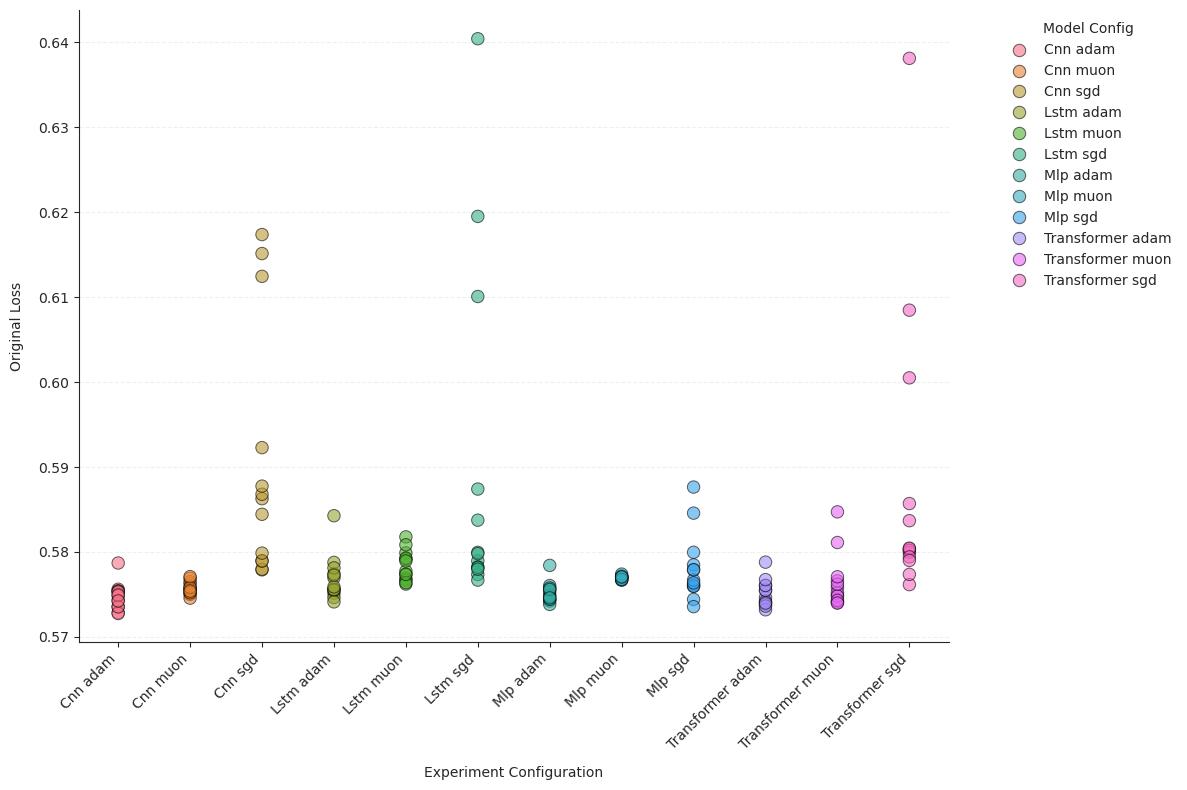
To ensure robustness, we repeat the training procedure for every architecture–optimizer pair using $N=13$ distinct random seeds for initialization and data shuffling. Table 1 reports the mean NMSE and its standard deviation across seeds. Two facts emerge:

• Linearity dominates performance metrics. Neural networks do not materially outperform linear benchmarks. OLS and LASSO achieve error levels statistically indistinguishable from even the most complex Transformer models.

• Loss-level ties persist across training pipelines. Across optimizers, NMSE differences are small. While SGD is on average slightly worse and exhibits occasional outlier runs, aggregate error alone remains largely uninformative for distinguishing among the learned predictors.

These results imply that, under conventional performance metrics, all learning systems considered are observationally equivalent. However, this equivalence is fragile: we will see that this loss-level equivalence does not imply functional or decision-level equivalence.

3.2 Robustness via Hyperparameter Optimization

A potential concern in comparing optimization algorithms is that performance parity may arise from suboptimal tuning of one or both methods. To rule this out, we perform a rigorous hyperparameter optimization for every architecture–optimizer pair using the Optuna framework (Akiba et al., 2019).

We search step sizes $\eta$ over the range $[10^{-5},10^{-1}]$ for all optimizers. For weight decay $\lambda$, we employ distinct ranges: $[10^{-5},1]$ for SGD, $[10^{-4},10^{-1}]$ for Adam, and $[10^{-5},5]$ for Muon, consistent with our empirical observation that the latter requires significantly stronger regularization to achieve optimal performance. For each architecture–optimizer pair, we select the configuration that minimizes the validation loss.

The results reported in Table 1 reflect these optimally tuned models. Strikingly, even under this idealized comparison, performance remains statistically indistinguishable across architectures and optimizers. Hyperparameter optimization therefore fails to break the leaderboard tie, in contrast to what is commonly observed in vision and language tasks.

Taken together, these findings rule out poor tuning as an explanation for performance parity.

4 Functional Divergence via Optimization

Section 3 establishes that all architecture–optimizer pairs are statistically indistinguishable under standard loss-based evaluation. Unlike vision or NLP, where optimizers induce meaningful generalization differences, test loss here remains invariant. We show that this predictive equivalence masks deep heterogeneity: qualitatively distinct predictors remain equally compatible with the data, a phenomenon related to underspecification and predictive multiplicity (see Appendix G).

We directly investigate the functions learned by each pair $(\mathcal{A},\mathcal{O})$, selecting the optimal model identified via hyperparameter tuning. Holding architecture fixed, we demonstrate that the choice of optimizer acts as a powerful source of inductive bias, selecting qualitatively different decision rules from the same hypothesis class. We refer to this phenomenon as functional divergence: models that are metrically equivalent in terms of predictive error, yet geometrically and economically distinct in how they map past information into forecasts.

4.1 Functional Divergence

Figure 2: Functional Divergence: Adaptive vs. SGD. Impulse response analysis of the CNN architecture at Lag $t-1$. The optimizer dictates the complexity of the learned function: Adam and Muon (Blue/Red) identify a complex non-linear dampening mechanism, whereas SGD (Green) reverts to a distinctively different function. All models achieve comparable predictive error, yet represent fundamentally different functional interpretations of the same data.

(a) LSTM Surface.

(b) CNN Surface.

(c) Transformer Surface.

Figure 3: Functional Divergence Across Architectures. The difference surface $D=\hat{y}_{\text{Muon}}-\hat{y}_{\text{Adam}}$ plotted for LSTM (left), CNN (middle), and Transformer (right). All three architectures produce complex, non-flat difference landscapes, confirming that Adam and Muon settle into fundamentally different local minima regardless of the specific architecture used.

To visualize the functional differences we employ Impulse Response Analysis $\mathcal{R}(k,\delta)$. Applying this diagnostic to the CNN architecture reveals optimizer-dependent divergence at lag $t-1$, as visualized in Figure 2 (extended results in Appendix D). More generally, we observe that:

• SGD tends to simpler solutions: SGD produces a flatter response surface.

• Adaptive Methods learn nonlinear functions: Adam and Muon converge to sigmoidal response surfaces, learning to dampen extreme volatility shocks.

Most importantly, this functional divergence is pervasive across architectures. Figures 3(a), 3(b), and 3(c) plot the Difference Surface $D(x)=\hat{y}_{\text{Muon}}(x)-\hat{y}_{\text{Adam}}(x)$ for the LSTM, CNN, and Transformer, respectively. In all three cases, the surfaces are highly structured and non-planar. This indicates that the optimizers disagree on the geometric interaction of input lags regardless of the architectural constraints.

Functional divergence is not a seed artifact.

Training neural networks is stochastic (initialization and mini-batch order), so a natural concern is that the functional differences in Figures 2–3 reflect idiosyncratic run-to-run variation rather than a systematic optimizer effect. Two observations argue against this interpretation. First, the optimizer-difference surfaces are highly structured and different across multiple architectures (Figure 3), exhibiting coherent geometric patterns rather than the unstructured fluctuations one would expect from pure seed noise. Second, the optimizer-swap interventions provide direct evidence of optimizer-dependent attractors. Starting from the same trained weights, switching from Adam to SGD causes the response profile to rapidly collapse toward the characteristic SGD solution, becoming indistinguishable from a baseline SGD run (Figure 6). Conversely, initializing Adam from an SGD solution restores Adam-looking functionals.

4.2 Optimizer-Driven Feature Attribution

(a) CNN feature importance.

(b) LSTM feature importance.

Figure 4: Mechanism of Divergence (SHAP Values). Feature attribution analysis comparing Adam and Muon optimizers across lags $t-1$ (Feature 99) to $t-100$ (Feature 0).

To understand the origin of these functional differences, we analyze feature attribution using SHAP (Lundberg & Lee, 2017). The following results reveal that optimizer choice fundamentally alters the lag-importance profile of the model.

For CNNs (Figure 4(a)), the architecture appears to be more important than the optimization path for feature selection. Adam, Muon, and SGD all place primary emphasis on the most recent lags (Features 96-99), and followed to the same distant lags (Features 36-38). However, for LSTMs (Figure 4(b)), where the theoretical receptive field is unbounded, the optimizer becomes the selection mechanism. Muon facilitates the exploitation of long-term memory, while Adam concentrates on recent history, effectively underutilizing the recurrent structure of the architecture. Consistent with its tendency toward simpler solutions, SGD restricts its attention almost exclusively to the most recent lags across both architectures. This reversal indicates that temporal dependence is not solely a property of the architecture (LSTM vs. CNN), but an emergent property of the optimization trajectory.

From a financial perspective, these differences in temporal weighting admit a natural interpretation. Emphasis on very recent lags corresponds to short-horizon volatility dynamics driven by microstructure effects, order flow, and volatility clustering (Engle, 1982), while attention to longer horizons reflects the influence of slower-moving information such as earnings announcements or other scheduled disclosures (Andersen et al., 2007). The fact that some optimizers systematically recover a quarterly lag structure, while others suppress it entirely, suggests that optimizer choice implicitly selects among competing economic explanations for volatility persistence.

While observationally equivalent under standard loss, these distinct lag profiles imply contradictory economic beliefs about the source and stability of volatility. Consequently, the optimizer does not merely affect interpretability, but implicitly encodes specific views on how information propagates through financial markets.

4.3 Mechanism: Curvature Constraints

Figure 5: Edge of Stability Trace under SGD. Evolution of the maximum Hessian eigenvalue $\lambda_{max}$ during SGD training for the MLP architecture relative to the stability threshold $2/\eta$. Sharpness rises until it equilibrates at the edge of instability. Financial neural networks exhibit EoS behavior where sharpness tracks the stability limit.

Why do these optimizers induce functional divergence? Here, we investigate the mechanism associated with the selection of different predictors by different optimizers. Additional experimental details are provided in Appendix E.

The Edge of Stability. First, we confirm that financial neural networks exhibit Edge of (Stochastic) Stability (EoSS) dynamics (Jastrzębski et al., 2019, 2020; Cohen et al., 2022b, a, 2024; Andreyev & Beneventano, 2025). As shown by our diagnostics (Figure 5), during SGD training the curvature (top Hessian eigenvalue $\lambda_{max}$) increases until it reaches the stability threshold $2/\eta$ and subsequently stabilizes.

Using a novel dataset scaling analysis (detailed in Appendix E.1), we estimate that the stability horizon for the full dataset extends to approximately $130,000$ steps ($\approx 29$ epochs). Since our optimally tuned models are trained for $50$ epochs, we conjecture that the observed functional divergence might be associated to the constraint imposed by EoSS on the optimization trajectories, which differ across optimizers.

Empirical observations.

Optimizers consistently exhibit distinct geometric biases and learning patterns:

• SGD tends to settle in flatter regions and finds simpler solutions.

• Adaptive methods (like Adam) effectively “flatten” the optimization landscape via preconditioning, allowing the optimizer to stably descend into narrow valleys (high original curvature) that are inaccessible to SGD.

Note that the observation that SGD stabilizes in flatter regions than Adam has already been established in vision and language tasks(Cohen et al., 2022a); its novelty here lies in the context of financial time series. To quantify this, we compute the maximum Hessian eigenvalue ($\lambda_{max}$) at convergence for both CNN and MLP models. Comparing solutions obtained using the optimizer-specific optimal learning rates (approximately $2\cdot 10^{-4}$ for Adam vs $5\cdot 10^{-2}$ for SGD), we observe a systematic sharpness gap:

• MLP: Adam ($\lambda_{max}\approx 111.5$) $>$ SGD ($\lambda_{max}\approx 63.1$)

• CNN: Adam ($\lambda_{max}\approx 239.9$) $\gg$ SGD ($\lambda_{max}\approx 51.5$)

Across architectures, Adam converges to solutions solutions that are significantly sharper ($2-5\times$) than those obtained by SGD. We further observe that this sharpness pattern couples with the functional differences documented in Figure 2 for financial time series: complex functional features (such as precise long-term memory or non-linear dampening) co-occur with sharper solutions.

Importantly, we do not claim causality, nor do we assert that this phenomenon generalizes beyond the present task. Further work is needed to assess its relevance in financial time series more broadly.

Intervention Experiments.

Figure 6: Optimizer Intervention. Response profiles when swapping optimizers after convergence. (Blue) Starting from a complex Adam model, SGD forces a collapse to a simpler solution. (Orange) Starting from a piecewise linear SGD model, Adam recovers the non-linear complexity.

Figure 7: Early Intervention (Warm Start). The difference surface between the Early-Swap model (Adam $\to$ SGD at step 500) and the Baseline SGD model. The surface is effectively flat ($D\approx 0$), confirming that even with an early "Adam push," the model gravitates entirely to the simpler SGD attractor.

To better assess at which phase of training this functional divergence emerges, we perform intervention experiments in which optimizer configurations are swapped at different training stages (see Appendix E.6 for the details).

First, we perform a late intervention (Figure 6), initializing SGD with the weights of a fully converged Adam model. Under SGD, the model rapidly drifts away from this solution, reverting towards a less curved profile ($\text{Adam}\to\text{SGD}$) that is indistinguishable from the baseline SGD solution. This phenomenon indicates that the complex minima found by Adam are repulsive under the geometry of the SGD update, echoing the catapult effect of SGD at instability highlighted by (Andreyev & Beneventano, 2025). Conversely, when Adam is initialized with the linear weights of a converged SGD model, the model rapidly recovers functional complexity, and the curvature increases.

Second, we perform an early intervention, switching from Adam to SGD after only 500 steps. We hypothesize that if Adam merely helps navigate a difficult initial loss landscape, this “warm start" might allow SGD to eventually settle into a complex minimum. However, we observe the opposite: the difference surface between the Early-Swap model and the baseline SGD model is effectively zero (Figure 7).

These intervention experiments solidify our conjecture that the co-occurrence of solution flatness and function simplicity reflects a correspondence, at least within the scope of our empirical setting. Moreover, they suggest that the late-training phase at the EoSS is enough to motivate functional divergence and that EoSS-induced spikes may be associated with subsequent model simplification, thereby linking the two phenomena.

4.4 Verification via Ensembling

While a lack of ensemble improvement is hard to interpret (it may reflect shared bias or highly aligned errors), a clear gain is more informative. If the averaged model strictly outperforms its members under NMSE, then – by the ambiguity decomposition (Krogh & Vedelsby, 1994) – the predictors must disagree on a non-negligible set of inputs, i.e., their errors are not perfectly aligned. This indicates the models have learned non-identical functions on the data distribution.

We construct a heterogeneous ensemble across optimizers:

$$\hat{y}_{\text{ens}}=\frac{1}{3}\left(\hat{y}_{\text{CNN, Adam}}+\hat{y}_{\text{MLP, Muon}}+\hat{y}_{\text{MLP, SGD}}\right).$$ (3)

This ensemble achieves an out-of-sample NMSE of 0.5730. This strictly dominates the OLS baseline (0.5751) and outperforming each constituent in the same ensemble set.

The fact that combining “metrically equivalent" models reduces error, implies that their prediction errors are not perfectly aligned. This confirms our hypothesis: the pairs $(\mathcal{A},\mathcal{O})$ are not redundant; they implement non-identical predictors whose differences are complementary and yield a measurable reduction in generalization error.

Taken together, these results establish that predictive equivalence under standard loss metrics conceals substantial heterogeneity in the learned functions. Optimizer choice systematically shapes curvature, temporal dependence, and functional form, even when architectures and predictive accuracy are held fixed. As a result, models that are observationally equivalent from a machine learning perspective encode meaningfully different representations of the data-generating process. The natural next question is whether such hidden functional differences matter for downstream use.

5 Behavioral Divergence in Trading Strategies

In this section, we shift attention to the financial implications of functional divergence, showing that differences invisible to standard loss-based metrics can translate into distinct trading and portfolio decision rules. Recent work has emphasized that predictive accuracy alone is insufficient for model selection when downstream decisions and interpretability are considered (Rudin et al., 2022; Fisher et al., 2019). Departing from standard benchmarking studies that focus on marginal performance improvements (see Appendix G), we demonstrate that metrically equivalent predictors can induce economically distinct behavior through optimizer-driven differences in functional form.

We document a form of decision multiplicity that is invisible to standard evaluation metrics. The analysis is not intended as a performance evaluation or asset-pricing test, but as a diagnostic of how metrically equivalent predictors differ in implementability. Methodological details are provided in Appendix F.

Figure 8: Sharpe–Turnover Frontier across Volatility Quintiles. Each point corresponds to a volatility model embedded in a volatility-managed portfolio rule. Panel (a) reports the low-volatility portfolio (Q1) and panel (b) the high-volatility portfolio (Q5). Across both quintiles, Sharpe ratios are broadly similar across models, while induced turnover varies substantially with architecture and optimizer choice, implying that metrically equivalent predictors can yield markedly different trading behavior.

We construct volatility-managed portfolios and report the resulting Sharpe–Turnover frontier in Figure 8. Differences in turnover reflect responsiveness rather than smoothness: while adaptive optimizers learn dampened, nonlinear impulse responses in isolation, they also produce forecasts that are more locally sensitive to small changes in the input state, leading to more frequent rank reversals when embedded in allocation rules. As a result, Adam- and Muon-trained models induce average higher turnover despite having similar predictive accuracy.

By contrast, SGD tends to select simpler, more stable volatility rankings over time. This reduced sensitivity translates into lower trading frequency and lower turnover, even when Sharpe ratios are statistically indistinguishable across optimizers. Optimizer choice therefore primarily affects implementability, reinforcing the distinction between predictive equivalence and behavioral equivalence.

The key takeaway of this section is that in underspecified environments, economic outcomes depend on which admissible function is selected, not on predictive accuracy alone. As a result, model evaluation should account for stability and implementability alongside error-based metrics. While gross Sharpe ratios are comparable, the effective utility of these models differs once transaction costs are applied. The excess turnover generated by adaptive-optimizer-based models erodes returns. Thus, in a realistic trading environment, the optimizer effectively determines the capacity and viability of the strategy.

6 Conclusion

Predictive equivalence is real—and misleading.

Financial volatility forecasting lives in a Rashomon regime: across architectures and optimizers, predictors often tie under conventional error metrics. But tied NMSE does not imply tied functions. Impulse-response profiles, optimizer-difference surfaces, and lag attributions reveal materially different input–output mappings, which translate into different stability and turnover once forecasts are embedded into trading rules.

Question 1 (interchangeability / “should we use deep nets?”).

No: tied predictors are not interchangeable, because “same loss” need not mean “same behavior” downstream. Yes: deep networks still matter—not as leaderboard winners, but as flexible hypothesis classes that realize a menu of admissible signals (stable vs. reactive, smooth vs. aggressive, short- vs. long-memory).

Question 2 (“is the optimizer just engineering?”).

No. When loss is indifferent, optimization is an implicit prior: holding data, architecture, and scalar error fixed, the optimizer selects which admissible function is returned, often determining implementability (e.g., turnover) even when predictive accuracy is unchanged.

Takeaway.

In underspecified time series, model selection is function selection. When the leaderboard is a tie, choose the function that matches the downstream economic objective—or the optimizer will choose it for you. In finance, the optimizer is part of the model.

Impact Statement

This work highlights the limitations of scalar loss metrics for model selection in low-signal domains. We demonstrate that optimization choices induce functional divergence despite predictive equivalence, introducing hidden variations in downstream decision-making. These findings suggest that benchmarking in underspecified regimes should integrate behavioral stability and induced economic consequences alongside generalization error. This perspective is relevant for the reliable deployment of machine learning in finance and other high-noise environments.

Appendix

Appendix A Choosing a Dataset

As a Gedankenexperiment, we postulate the ideal characteristics a dataset should possess:

• Reliability and provenance. Data are free of obvious errors, typos, and measurement artifacts; missing values are minimal, explicitly flagged, and documented. Units, definitions, and formats are consistent across series and over the full time span. The origin and transformation pipeline are transparent and traceable to reputable sources.

• Temporal and cross-sectional breadth. Time series are sufficiently long to span multiple economic regimes and market cycles (e.g., bull and bear markets, recessions, high/low inflation). The cross-section is large (e.g., hundreds of securities rather than a handful), and each timestamp includes a rich feature set beyond prices alone.

• Diversity with low average correlation. The universe covers heterogeneous exposures to known risk factors (e.g., value vs. growth, small- vs. large-cap, high vs. low volatility) and a broad range of industries (technology, healthcare, energy, financials, etc.), reducing concentration risk and cross-series redundancy.

• Modeling readiness. The provided variables, or standard transformations (e.g., returns), are reasonably stationary, or the dataset includes guidance to achieve stationarity. The predictive task is clearly defined, with one or more precomputed target variables. Standardized training/validation/test splits and a baseline training protocol are supplied for reproducibility and fair comparison.

Synthetic Data

de Prado (2018); Yoon et al. (2019) propose using synthetic time series, respectively for backtesting/robustness and for training/evaluation via TSTR. While such data are useful for stress testing and mitigating overfitting, a benchmark’s purpose is to assess performance against real market outcomes. Hence, we contend that synthetic data are not an appropriate benchmarking substrate, for the following reasons:

1. Benchmarking aims at reality. The primary purpose of a benchmark is to assess a model’s performance against real market outcomes. Synthetic data are, by construction, a simplified and incomplete model of that reality.

2. Model-implied worlds. A synthetic generator is calibrated to statistical regularities observed in historical data. It cannot, by definition, reproduce dynamics that are absent from (or misspecified in) its data-generating assumptions.

3. Validity is conditional on the generator. Superior performance on synthetic data merely demonstrates skill at exploiting the rules of the generator, not the market. This invites specification-led overfitting.

4. Structural breaks are not authentically captured. While one can program regime shifts by changing generator parameters, that does not replicate unforeseen changes in market logic (i.e., true structural breaks). For instance, the post-2008 era of quantitative easing altered cross-asset correlations and the risk-free rate regime in ways not anticipated by pre-crisis models.

In short, optimizing to a synthetic world risks tailoring models to the generator’s quirks rather than to markets, undermining external validity as a benchmark.

The Closest Real Dataset to the Ideal Dataset

We propose a dataset constructed from the Center for Research in Security Prices (CRSP), focusing on daily observations of S&P 500 constituents. The construction aligns with the ideal characteristics outlined above:

• Reliability and provenance. The dataset is sourced exclusively from CRSP, the institutional standard for academic financial research in the United States, whose data undergo rigorous cleaning and validation. Our construction—joining the CRSP Daily Stock File (DSF) with the S&P 500 constituents list (msp500list)—is explicit and reproducible. By using historical membership windows, it correctly handles index composition changes and therefore avoids survivorship bias.

• Temporal and cross-sectional breadth. The sample spans from January 2000 to the December 2024, covering multiple recessions (1990, 2001, 2008, 2020), the dot-com boom and bust, and a secular decline followed by a rise in interest rates. The cross-section comprises all securities during their tenure in the S&P 500 (roughly 500 at any time). Each observation includes not only the close but also open, high, and low prices, trading volume, and the adjustment factors needed to reflect corporate actions.

• Diversity with low average correlation. The S&P 500 is a diversified benchmark spanning all major GICS sectors of the U.S. economy. Its inclusion criteria yield leading, highly liquid firms with heterogeneous exposures (growth vs. value, differing risk profiles) and a large-cap tilt. Tracking constituent histories captures the evolving sectoral and factor composition of the U.S. market.

Appendix B Data Diagnostics and Descriptive Checks

Our working panel contains 3,155,303 daily observations drawn from CRSP for S&P 500 constituents between January 2000 and December 2024. Each row corresponds to a PERMNO–date pair and includes returns and standard OHLCV fields plus CRSP adjustment factors (Table A1). Figures A1–A3 summarize sectoral coverage, firm size, and cross-sectional dependence.

Table A1: Core variables in the analysis dataset

Variable	Description
PERMNO	CRSP permanent security identifier
date	Trading day (NYSE calendar)
ret	Daily return (CRSP; split/dividend adjusted)
open, high, low, close	Daily O/H/L/C prices
vol	Daily share volume
cfacpr	Price adjustment factor for corporate actions

Figure A1: Distribution of observation counts by GICS sector.

The sample is balanced: Financials, Consumer Discretionary, Industrials, Information Technology, and Health Care account for most rows, with no sector too concentrated, and all sectors well represented.

B.1 Firm Size: Market Capitalization

Figure A2: Yearly $\log_{10}$ distribution of average market capitalization per stock.

As expected for S&P 500 constituents, capitalization levels are high and, within year, approximately normal on the log scale, with a right tail of very large firms in the latest years (Magnificent 7 effect). The panels show a stable center with modest cyclical shifts across regimes.

B.2 Cross-Sectional Dependence

Figure A3: Upper-triangular correlation matrices of daily returns by year.

Correlations are moderate and time-varying: higher in crisis/high-volatility periods (ex: 2008, 2011, 2020) and lower in calmer years, consistent with standard co-movement dynamics—supporting models with time-varying dependence.

B.3 Reproducibility Notes

All series are pulled directly from CRSP using the WRDS Python API, using the following query:

⬇

SELECT

s.permno,

s.date,

s.ret,

s.prc AS close,

s.vol,

s.openprc AS open,

s.askhi AS high,

s.bidlo AS low,

s.cfacpr

FROM crsp.dsf AS s

JOIN crsp.msp500list AS m

ON s.permno = m.permno

WHERE s.date BETWEEN GREATEST(m.start, DATE ’2000-01-01’)

AND LEAST(m.ending, DATE ’2024-12-31’)

ORDER BY s.permno, s.date;

Appendix C Implementation and Experimental Setup

We employ the Garman-Klass estimator to compute a daily realized-variance proxy from OHLC data. We partition the dataset into training, validation, and test sets following a chronological split with a ratio of 3:1:1.

To ensure numerical stability and mitigate the impact of extreme outliers (some exceeding 300 standard deviations), we apply per-asset winsorization using training-set quantiles:

$$x\leftarrow\min\!\big(\max(x,\,q_{0.5\%}^{\text{train}}),\,q_{99.5\%}^{\text{train}}\big).$$

Subsequently, the values are annualized (scaled by 252) and standardized via z-score normalization using the mean and standard deviation of the training set:

$$x\leftarrow\frac{x-\mu_{\text{train}}}{\sigma_{\text{train}}}.$$

The final input vector comprises the processed log-variances $\mathbf{x}_{t}=(\widehat{\sigma}^{2}_{t-L},\ldots,\widehat{\sigma}^{2}_{t})$ used to predict the next-day log-variance $y_{t}$. We use $L=100$

C.1 Model Architectures

We evaluate four distinct deep learning architectures. All models share a consistent fine-tuning protocol focused on the learning rate and weight decay.

• LSTM: We utilize a stacked LSTM with 2 layers of 256 hidden units each. We employ the hidden state of the last time step for prediction (readout: last). To preserve signal integrity, we disable dropout and bidirectional processing.

• CNN: The convolutional network consists of three 1D-convolution blocks with channel sizes $[64,128,256]$, a kernel size of 8, and padding of 1. We use ReLU activation and Adaptive Average Pooling ($k=16$). The output is flattened and passed through an MLP head with sizes $[512,256]$.

• MLP: A pure Multilayer Perceptron baseline consisting of four fully connected layers with sizes $[512,256,256,128]$ and ReLU activations.

• Transformer: We use an encoder-only Transformer with $L=2$ layers, model dimension $d_{\text{model}}=128$, and $h=8$ attention heads. Inputs are projected to $d_{\text{model}}$ and combined with learned positional embeddings. The sequence representation is aggregated via mean pooling (readout: mean) and passed to an MLP prediction head with sizes $[128,64]$.

C.2 Linear Baselines

In addition to deep learning models, we evaluate two linear baselines.

• OLS: We implement Ordinary Least Squares regression using statsmodels, computing the weights directly via the closed-form analytical solution.

• LASSO: We employ Least Absolute Shrinkage and Selection Operator regression via scikit-learn. The penalization parameter is tuned via grid search over $\alpha\in[0.001,0.01,0.025,0.05,0.1,0.25]$. We select the $\alpha$ that minimizes the validation loss. Consistent with our general protocol, the final model is refitted on the combined training and validation sets using the optimal $\alpha$.

C.3 Training and Optimization

Hyperparameters, specifically weight decay and learning rate, are tuned using the fixed validation set. For each combination of architecture and optimizer, we select the hyperparameter configuration that minimizes the validation loss. We optimize the Mean Squared Error (MSE) using Adam, SGD, and Muon optimizers with a batch size of 512. To prevent overfitting, we employ an early stopping mechanism that terminates training if the validation loss does not improve for 10 consecutive epochs. Finally, to maximize data utilization, we merge the training and validation sets and retrain the final models on this combined dataset using the selected optimal hyperparameters and the optimal number of epochs identified during validation.

C.4 Robustness Protocol:

All neural network experiments were repeated $13$ times using different fixed random seeds, affecting weight initialization and batch shuffling. Linear baselines (OLS, LASSO) are deterministic given the fixed training set. The reported functional diagnostics (SHAP, Impulse Response) correspond to the seed yielding the median validation loss to ensure the analyzed model is representative of the central tendency of the optimization dynamics.

To ensure that the predictive equivalence observed in Table 1 is not an artifact of aggregation, we visualize the full distribution of Out-of-Sample NMSE across all 13 random seeds in Figure A4.

Figure A4: Distribution of Test Error. Box plots showing the spread of NMSE across 13 independent runs for each Architecture-Optimizer pair. SGD exhibits heavier-tail variability with occasional outliers.

Appendix D Functional Divergence Analysis

(a) CNN Feature Attribution

(b) LSTM Feature Attribution

(c) MLP Feature Attribution

(d) Transformer Feature Attribution

Figure A5: Optimizer-Driven Feature Attribution (SHAP). Comparison of lag importance across architectures.

Figure A6: Linear Baselines. Coefficients of OLS and LASSO regressions for 100 lagged squared volatility terms ($\sigma^{2}_{t-99}$ through $\sigma^{2}_{t}$). Note the sparsity of LASSO versus the dense allocation of OLS.

(a) CNN Impulse Response

(b) LSTM Impulse Response

(c) MLP Impulse Response

(d) Transformer Impulse Response

Figure A7: Functional Divergence (Impulse Responses). Comparison of model sensitivity at $t-1$ across optimizers.

(a) Adam

(b) Muon

(c) SGD

Figure A8: Response Surfaces for CNN Architecture. Comparing the learned decision boundaries across optimizers.

(a) Adam

(b) Muon

(c) SGD

Figure A9: Response Surfaces for LSTM Architecture. Comparing the learned decision boundaries across optimizers.

(a) Adam

(b) Muon

(c) SGD

Figure A10: Response Surfaces for MLP Architecture. Comparing the learned decision boundaries across optimizers.

(a) Adam

(b) Muon

(c) SGD

Figure A11: Response Surfaces for Transformer Architecture. Comparing the learned decision boundaries across optimizers.

Appendix E Search for a Mechanism

In this section, we provide the detailed experimental protocols for the Edge of Stability and the optimizer intervention experiments described in Section 4.3.

E.1 The Edge of Stability as a Constraint on the Dynamics

We introduced the Edge of (Stochastic) Stability (EoS/EoSS) viewpoint in Appendix G. Here we add a complementary dynamical interpretation that is useful for reading the sharpness traces in Figure 5: once training approaches the stability boundary, stability becomes an active constraint on the trajectory.

Stable set and stability boundary.

For concreteness, consider (full-batch) gradient descent on a loss $L(\theta)$ with step size $\eta$, $\theta_{t+1}=\theta_{t}-\eta\nabla L(\theta_{t})$. Linearizing around $\theta_{t}$ yields perturbation dynamics $\delta_{t+1}\approx(I-\eta H_{t})\delta_{t}$ with $H_{t}=\nabla^{2}L(\theta_{t})$, and a standard local quadratic sufficient condition for stability is $\eta\lambda_{\max}(H_{t})\lesssim 2$. This motivates defining a stable set at step size $\eta$ as

$$\mathcal{S}_{\eta}\;:=\;\left\{\theta:\;(2/\eta)I-\nabla^{2}L(\theta)\succeq 0\right\}.$$ (4)

Training that enters an EoS-like regime can be understood as repeatedly interacting with (and self-stabilizing around) the boundary of $\mathcal{S}_{\eta}$.

Central flow: EoS as a constrained dynamics.

A precise formalization of the “constraint” intuition is given by the central flow approximation. The central-flow perspective defines a smooth projected gradient flow that evolves like gradient descent while remaining in the stable set $\mathcal{S}_{\eta}$. Concretely, Cohen et al. (2024) define Gradient Descent Central Flow as a projected gradient flow constrained to $\mathcal{S}_{\eta}$ and show that its Euler discretization recovers the discrete GD iterates. Empirically, central flow closely tracks the time-averaged GD trajectory deep into the EoS regime. This makes the constraint interpretation explicit: once the trajectory reaches the boundary, progress along the sharpest directions is no longer “free” and is continually corrected by the stability constraint.

Why this viewpoint matters for learning (and for optimizer comparisons).

The constraint view is valuable because it links curvature to which improvements are reachable in finite time. Recent work on stability as “complexity control” argues that EoS/EoSS effectively restricts the set of reachable parameter paths (and therefore the effective hypothesis class explored by training), thereby inducing an inductive bias over the learned function. That work also motivates studying stability through decompositions of the data distribution: hard examples and geometric outliers can disproportionately affect optimization dynamics, including curvature spikes and instability events, so the stability constraint can steer learning differently across inliers, boundary points, and outlier-like subsets. Finally, an important implication for our setting is that the stability constraint is optimizer-dependent: different optimizers “perceive” curvature differently (e.g., via preconditioning), and therefore interact with different effective stability boundaries. This provides a principled mechanism by which optimizer choice can select among multiple admissible predictors even when aggregate predictive loss ties.

E.2 Spikes Signal Edge of Stochastic Stability

In mini-batch training, the deterministic EoS picture above must be refined: for stochastic gradient methods, instability is driven by the interaction between curvature and sampling noise. The Edge of Stochastic Stability (EoSS) framework in Andreyev & Beneventano (2025) formalizes this point and provides an operational explanation for spikes in loss/curvature traces.

Batch sharpness as the stochastic stability quantity.

A key message of Andreyev & Beneventano (2025) is that for mini-batch SGD, the relevant stability quantity is not necessarily the top eigenvalue of the full-batch Hessian, but a stochastic analogue called batch sharpness. Batch sharpness is defined as an expected Rayleigh quotient of the mini-batch Hessian along the mini-batch gradient direction:

$$\mathrm{BS}(\theta)\;:=\;\mathbb{E}_{B}\!\left[\frac{\langle\nabla L_{B}(\theta),\,H_{B}(\theta)\,\nabla L_{B}(\theta)\rangle}{\|\nabla L_{B}(\theta)\|_{2}^{2}}\right],$$ (5)

where $\nabla L_{B}$ and $H_{B}$ are the gradient and Hessian of the mini-batch loss. Empirically, Andreyev & Beneventano (2025) argue that batch sharpness exhibits progressive sharpening and stabilizes near the boundary $2/\eta$ (largely independent of batch size), while the top eigenvalue of the full-batch Hessian can remain substantially below $2/\eta$.

Why spikes are diagnostic: instability $\Leftrightarrow$ catapults $\Leftrightarrow$ loss spikes.

Crucially, Andreyev & Beneventano (2025) propose that the “edge” should be defined through instability rather than oscillations alone. On a local quadratic model, they show that three phenomena essentially coincide: (i) breaking a valid instability criterion, (ii) a “catapult” event (a large overshoot driven by the sharpest direction), and (iii) a loss spike of sufficient magnitude. This yields an operational signature of EoSS: if a valid instability criterion is saturated along a trajectory, then a small destabilizing hyperparameter perturbation (e.g., increasing $\eta$ or decreasing batch size) should trigger catapults and the associated loss spikes, whereas the same perturbation is benign earlier in training.

Mechanism of spikes under EoSS.

Even when the expected batch sharpness sits near $2/\eta$, stochasticity implies that some mini-batches can have anomalously large directional curvature. A short run of such batches can temporarily push the iterate across the stability boundary, producing a catapult and a pronounced spike in loss; after the spike, the trajectory either diverges or re-enters a region where the instability criterion falls below threshold and progressive sharpening resumes. In our experiments, we therefore treat pronounced spikes in sharpness/loss traces as evidence that training has reached (or transiently crossed) the EoSS boundary, and we use optimizer-swap interventions as complementary probes that move the iterate between regions that are dynamically stable/unstable under a given update geometry.

E.3 Methodology: Scaling Laws for Stability Thresholds

The complexity of the power iteration necessary to estimate $\lambda_{\max}$ scales with the product of the dimensionality of model parameters and the size of the dataset. For this reason, it is infeasible to compute the curvature along the training trajectory with the full dataset. Consequently, we search for a scaling law of the entry point and we extrapolate over this law. Further work is needed to address whether this method is theoretically plausible.

We estimate the entry point into the EoS regime by exploiting the scaling properties of financial data. We postulate that the number of optimization steps $t^{*}$ required to reach the edge of stability follows a power law with respect to the dataset size $D$:

$$t^{*}(D)\approx\alpha\cdot D^{\beta}$$ (6)

To estimate the parameters $\alpha$ and $\beta$, we perform the following procedure:

1. Sub-sampling: We construct subsets of the training data with sizes $D\in\{16384,65536,131072,262144\}$.

2. Sharpness Monitoring: For each subset, we train an MLP using full-batch gradient descent (or large-batch SGD with equivalent noise scale) while monitoring $\lambda_{max}$ via power iteration.

3. Threshold Detection: We identify the critical step $t^{*}$ where the sharpness crosses the stability boundary:

   $$t^{*}=\min\{t:\lambda_{max}^{(t)}>2/\eta\}$$ (7)

E.4 Results and Extrapolation

The dynamics of this scaling are illustrated in Figure A12.

• Small Scale ($D=16k$) and ($D=65k$): The model enters the unstable regime rapidly, with $\lambda_{max}$ crossing $2/\eta$ early in training (approx. step 2,500 and 6,000 respectively).

• Medium Scale ($D=131k$): The stability duration extends significantly, delaying $t^{*}$ to approximately 18,000 steps.

• Large Scale ($D=262k$): In our largest subsample, the stability threshold is further pushed to $t^{*}\approx 32,000$ steps.

By fitting a linear regression to the log-log data of observed pairs $(D,t^{*})$ (see Figure 12(e)), we extrapolate the stability horizon for the merged train and validation dataset ($N\approx 2.3\times 10^{6}$). The projection yields an estimated entry point of $t^{*}\approx 130,000$ steps.

(a) Small Scale ($N=16k$)

(b) Medium Scale ($N=65k$)

(c) Large Scale ($N=131k$)

(d) Largest Scale ($N=262k$)

(e) Scaling Law Regression

Figure A12: Edge of Stability Scaling Analysis. Evolution of the Hessian spectral norm ($\lambda_{max}$) relative to the optimizer stability threshold ($2/\eta$). We observe a clear scaling law where increasing the dataset size $N$ delays the onset of the unstable, chaotic regime.

E.5 Verification of Stability

Our best-performing models (used for the functional divergence analysis in Section 4 are consistently selected at Epoch 50. Given our batch size of 512 and total $N\approx 2.3\times 10^{6}$, one epoch corresponds to $\approx 4,470$ steps.

• Model Selection Point: Epoch 40 $\approx 178,800$ steps.

• Estimated EoS Entry: $\approx 150,000$ steps.

The estimated entry point ($150k$) lies within the training horizon ($178k$). While extrapolation carries uncertainty, the proximity suggests the models likely traverse the EoS regime during the final epochs.

E.6 Intervention Experiments

To investigate the stability of the functional solutions found by SGD and Adam, and to determine whether their convergence to distinct minima is driven by the initialization basin or the optimizer’s update geometry, we performed intervention experiments involving the swapping of optimizers during training.

Optimizer Swap Protocol.

The transition between optimizers (e.g., $\text{Adam}\to\text{SGD}$) was implemented as a hard reset of the optimization state. This ensures that the subsequent trajectory is determined solely by the geometry of the target optimizer’s update rule, rather than by historical momentum accumulated by the previous optimizer. Specifically, at the intervention step $t_{\text{swap}}$:

1. Weights: The model parameters $\theta$ were initialized with the current weights from the source optimizer, such that $\theta_{\text{target}}^{(0)}=\theta_{\text{source}}^{(t_{\text{swap}})}$.

2. Optimizer State: The internal state of the target optimizer was initialized from scratch. For a swap to SGD, momentum buffers were zeroed. For a swap to Adam, the first and second moment estimates ($m_{t},v_{t}$) were reset to zero.

3. Hyperparameters: Upon swapping, the training continued using the specific hyperparameters (learning rate and weight decay) assigned to the target optimizer, as defined in the general experimental setup (Appendix C). This ensures that the target optimizer operates in its native regime rather than inheriting a potentially incompatible learning rate schedule.

Late Intervention (Stability Analysis).

For the late intervention experiments, we utilized fully converged models trained according to the standard procedure described in Appendix C. We extracted the weights $\theta^{*}$ resulting from the full training trajectory of the source optimizer and used them as the initialization for the target optimizer. The target optimizer was then run for a full training duration to observe whether the model would remain in the learned basin or drift toward a new attractor.

Early Intervention (Warm Start).

To test the hypothesis that Adam serves primarily to navigate initial saddle points, we performed an early swap at step $t_{\text{swap}}=500$. The model was trained with Adam for the first 500 steps to bypass initial training instability. At $t=500$, the optimizer was switched to SGD (following the reset protocol above). The model was then trained to full convergence following the standard duration and schedule described in Appendix C.

Appendix F Volatility-Managed Portfolios

This appendix reports additional details for the downstream portfolio experiment used to illustrate how optimizer-induced functional differences in volatility forecasts translate into differences in decision stability. The analysis is not intended as a performance benchmark, but as a diagnostic of the implementability of metrically equivalent predictors.

F.1 Cross-sectional implementation

Our primary implementation is cross-sectional. On each trading day, assets are sorted into quintiles based on predicted next-day volatility $\hat{\sigma}_{i,t}$. Within each quintile, portfolios are equal-weighted and reconstituted daily. We report results for all quintiles, with particular emphasis on the lowest and highest-volatility quintiles (Q1 vs Q5), whose composition is most sensitive to fluctuations in the volatility ranking and therefore most informative about signal stability.

F.2 Turnover and stability metrics

Portfolio turnover is computed as $\frac{1}{2}\sum_{i}\left|w_{i,t}-w_{i,t-1}\right|$, where $w_{i,t-1}$ refers to the realized weight immediately before rebalancing at time $t$, and averaged over time. Turnover provides a model-agnostic measure of signal smoothness and implied trading intensity, independent of transaction cost assumptions. In addition, we report standard risk and performance summaries (annualized return and volatility, Sharpe ratio, and maximum drawdown) to verify that differences in trading activity are not driven by trivial changes in portfolio risk exposure.

Table A2: Volatility-sorted portfolios. Performance and turnover of equal-weight portfolios formed on predicted volatility. Q1 denotes the lowest-volatility quintile; Q5 the highest.

Model	Ann. Ret.	Ann. Vol.	Sharpe	Max DD	Turnover
Q1: Low Volatility
OLS	0.120	0.130	0.921	-0.397	0.203
LASSO	0.119	0.130	0.917	-0.402	0.217
CNN (SGD)	0.117	0.129	0.906	-0.393	0.069
CNN (Muon)	0.124	0.129	0.959	-0.389	0.180
CNN (Adam)	0.117	0.130	0.898	-0.398	0.193
LSTM (SGD)	0.115	0.130	0.890	-0.413	0.162
LSTM (Muon)	0.121	0.129	0.938	-0.398	0.184
LSTM (Adam)	0.116	0.130	0.896	-0.395	0.196
MLP (SGD)	0.120	0.130	0.921	-0.397	0.208
MLP (Muon)	0.117	0.129	0.906	-0.390	0.149
MLP (Adam)	0.117	0.130	0.897	-0.397	0.190
Transformer (SGD)	0.117	0.130	0.902	-0.395	0.203
Transformer (Muon)	0.116	0.130	0.895	-0.392	0.194
Transformer (Adam)	0.119	0.130	0.914	-0.396	0.194
Q5: High Volatility
OLS	0.124	0.297	0.417	-0.718	0.150
LASSO	0.124	0.296	0.419	-0.717	0.163
CNN (SGD)	0.120	0.300	0.402	-0.718	0.059
CNN (Muon)	0.124	0.297	0.417	-0.684	0.143
CNN (Adam)	0.127	0.296	0.429	-0.703	0.157
LSTM (SGD)	0.123	0.297	0.416	-0.708	0.131
LSTM (Muon)	0.122	0.297	0.412	-0.706	0.148
LSTM (Adam)	0.123	0.296	0.416	-0.723	0.159
MLP (SGD)	0.124	0.296	0.420	-0.709	0.163
MLP (Muon)	0.123	0.299	0.411	-0.719	0.105
MLP (Adam)	0.125	0.297	0.422	-0.712	0.151
Transformer (SGD)	0.124	0.295	0.418	-0.717	0.166
Transformer (Muon)	0.125	0.295	0.421	-0.710	0.161
Transformer (Adam)	0.124	0.296	0.418	-0.716	0.161

F.3 Summary results

Table A2 reports performance and turnover metrics for volatility-sorted portfolios (Q1 and Q5) across model families and optimizers. Risk-adjusted performance is tightly clustered across specifications: Sharpe ratios vary only modestly within each quintile, and annualized volatility is nearly identical by construction.

By contrast, turnover exhibits substantial dispersion. In the Q1 portfolio, average daily turnover ranges from approximately 7% for CNN models trained with SGD to over 18–20% for Adam-trained neural networks and linear baselines. Similar, though slightly attenuated, patterns are observed in Q5. These differences arise despite nearly indistinguishable predictive accuracy, indicating that optimizer choice materially affects the stability of the induced volatility ranking rather than portfolio risk characteristics.

Figure A13: Rolling turnover of volatility rankings (Q1), averaged by optimizer. Turnover is computed for equal-weight daily volatility-quintile portfolios and shown as a rolling one-year average. Shaded regions denote major stress episodes.

F.4 Time-series evidence: turnover dynamics

Figure A13 plots rolling one-year turnover for the Q1 volatility-ranked portfolio, aggregated by optimizer class. The ordering observed in Table A2 is persistent over time: models trained with SGD consistently exhibit the lowest turnover, followed by Muon-trained ones, while Adam-trained models and linear baselines generate systematically higher trading intensity. These gaps widen during periods of market stress, suggesting that optimizer-induced differences in signal smoothness are amplified precisely when volatility dynamics are most unstable.

Figures A14–A16 provide complementary disaggregated evidence by reporting rolling six-month turnover for Q1, Q3, and Q5 ranked portfolios within each optimizer family. Within a fixed optimizer, differences across architectures are comparatively small, whereas differences across optimizers are pronounced. This pattern supports the interpretation that the optimizer, rather than the network architecture, is the primary driver of volatility ranking stability in this setting.

Together, these results confirm that even when predictive error is indistinguishable across models, the induced decision rules can differ sharply in their temporal stability. Optimizer choice therefore affects not only which function is learned, but also how reliably that function can be embedded into portfolio construction.

Figure A14: Rolling turnover by volatility quintile (Adam-trained models). Rolling six-month turnover for Q1/Q3/Q5 equal-weight portfolios formed by predicted volatility rankings.

Figure A15: Rolling turnover by volatility quintile (SGD-trained models). Rolling six-month turnover for Q1/Q3/Q5 equal-weight portfolios formed by predicted volatility rankings.

Figure A16: Rolling turnover by volatility quintile (Muon-trained models). Rolling six-month turnover for Q1/Q3/Q5 equal-weight portfolios formed by predicted volatility rankings.

Appendix G Further Related Work

Our work relates to several strands of literature on underspecification, optimization-induced inductive bias, interpretability, and empirical benchmarking in financial machine learning. While each of these literatures documents important facets of modern learning systems, they are rarely studied jointly in low signal-to-noise time-series environments.

G.1 Underspecification and Predictive Multiplicity

When the available data are only weakly informative about the target relationship, empirical risk minimization is best viewed as searching a landscape with a broad, shallow basin: many parameter settings sit on (nearly) the same “loss contour,” so the training objective does not single out a canonical predictor. This phenomenon has been formalized as underspecification (D’Amour et al., 2020): an ML pipeline (data, preprocessing, hypothesis class, optimizer, validation protocol) is underspecified when it can output many distinct predictors that are indistinguishable under in-distribution validation yet behave differently in deployment. Underspecification is closely related to Breiman’s Rashomon effect (Breiman, 2001), named after Kurosawa’s film in which multiple coherent narratives coexist without a single definitive truth (Kurosawa, 1950). The key methodological point is not merely that multiple models achieve similar error, but that the data do not refute many qualitatively different functional explanations.

Rashomon sets as a geometric object.

Fix a function class $\mathcal{F}$ and loss $\ell$. Writing $\widehat{R}_{n}(f)\!=\!\frac{1}{n}\sum_{i=1}^{n}\ell(f(x_{i}),y_{i})$ and $\widehat{R}_{n}^{\star}\!=\!\inf_{f\in\mathcal{F}}\widehat{R}_{n}(f)$, the (empirical) Rashomon set at tolerance $\varepsilon\!\geq\!0$ is

$$\mathcal{R}_{\varepsilon}(\mathcal{F})\;=\;\Bigl\{f\in\mathcal{F}\;:\;\widehat{R}_{n}(f)\leq\widehat{R}_{n}^{\star}+\varepsilon\Bigr\}.$$

In high-noise or intrinsically stochastic domains, $\mathcal{R}_{\varepsilon}(\mathcal{F})$ can be large even for small $\varepsilon$: recent results isolate regimes where noisy label generation provably induces large collections of near-optimal models (Semenova et al., 2023), and perspective work emphasizes that such multiplicity is common in high-stakes tabular settings (e.g., credit decisions, healthcare, criminal justice), precisely because the outcome mechanism is nondeterministic (Rudin et al., 2024). Moreover, a large Rashomon set is empirically and theoretically linked to the existence of simple-yet-accurate predictors (Semenova et al., 2022), contributing to the broader evidence that, on many tabular problems, high accuracy does not require black-box complexity (Holte, 1993; Lou et al., 2013; Angelino et al., 2018; McTavish et al., 2022; Liu et al., 2022b; McElfresh et al., 2023).

Near-optimal risk need not mean functional equivalence.

A central complication is that proximity in scalar risk does not control pointwise agreement. Two predictors can both lie in $\mathcal{R}_{\varepsilon}(\mathcal{F})$ and yet diverge sharply on individual instances, which is precisely the operational content of predictive multiplicity. In classification, one natural disagreement functional is

$$\mathrm{Dis}(f,g)\;=\;\mathbb{P}_{X\sim\mathcal{D}_{X}}\!\bigl[f(X)\neq g(X)\bigr],\qquad f,g\in\mathcal{R}_{\varepsilon}(\mathcal{F}),$$

and analogues for regression can track sign flips or threshold exceedances (e.g., $\mathbb{P}[\,|f(X)-g(X)|>\tau\,]$), which are often more decision-relevant than MSE. Predictive multiplicity has been explicitly quantified in classification (Marx et al., 2020) and broadened to procedural/justificatory concerns in policy-facing pipelines (Black et al., 2022). Importantly, the underlying observation that “many models fit about equally well” appears in older statistical and econometric discussions of model specification and competing adequate descriptions (Mountain & Hsiao, 1989; McCullagh & Nelder, 1989); what is comparatively less emphasized there is the downstream implication Breiman highlighted: if multiple distinct predictors induce different narratives (feature attributions, mechanisms, causal stories), then any single-model explanation is, without further structure, underdetermined by the data (Breiman, 2001; Marx et al., 2020).

Why we need behavioral evaluation beyond a single score.

These observations motivate evaluation protocols that treat a benchmark metric as necessary but not sufficient. Rather than interpreting a one-number gap (say, a tiny $\Delta$ in validation loss) as evidence of substantive superiority, one should ask how much behavioral latitude remains within $\mathcal{R}_{\varepsilon}(\mathcal{F})$:

• Stability of decisions: how large can $\mathrm{Dis}(f,g)$ be among near-optimal $f,g$? (Marx et al., 2020; Black et al., 2022)

• Stability of boundary geometry: how much can decision regions/threshold crossings move while preserving $\widehat{R}_{n}$? (Rudin et al., 2024)

• Constraint feasibility: does the Rashomon set contain models satisfying domain constraints (monotonicity, fairness, sparsity) without sacrificing accuracy? (Rudin et al., 2024)

Recent algorithms now make this viewpoint operational by explicitly representing or approximating Rashomon sets for nontrivial classes—including sparse decision trees, sparse GAMs, and risk scores—so that one can query the set for models that satisfy user preferences and examine variable importance across all good models, rather than conditioning on a single trained predictor (Xin et al., 2022; Zhong et al., 2023; Liu et al., 2022a; Zhu et al., 2023; Rudin et al., 2024).

Implications for financial forecasting.

Financial prediction problems are prototypical “noisy-label” regimes: outcomes are affected by latent factors and stochastic shocks, so it is natural to expect large Rashomon sets even when the modeling class is heavily restricted (Rudin et al., 2024; Semenova et al., 2023). Yet evaluation in finance often reduces model selection to a single scalar score (e.g., a loss, a correlation, or a portfolio-level summary), effectively projecting a high-dimensional behavioral object $\mathcal{R}_{\varepsilon}(\mathcal{F})$ onto one axis. The econometrics literature often responds to model uncertainty by combining forecasts (Timmermann, 2006); in contrast, we focus on a different question: when we must select a single predictor, which inductive biases (regularization, architecture, optimization, data processing choices) decide where we land within $\mathcal{R}_{\varepsilon}(\mathcal{F})$, and how that choice governs the stability of instance-level predictions, decision thresholds, and downstream actions under underspecification.

G.2 Implicit Bias of Optimization Trajectories

Changing optimizer or hyperparameters: same objective, different solutions.

A substantial literature documents that changing the optimizer (or its noise scale) can move learning toward different regions of parameter space with different curvature, geometry, and generalization behavior. Empirically, SGD-like methods are often associated with flatter solutions and better test performance than adaptive methods in high-signal domains (Wilson et al., 2017; Keskar et al., 2017), while adaptive optimizers can exhibit distinct “effective regularization” behavior unless properly regularized (notably via decoupled weight decay) (Loshchilov & Hutter, 2019; Zou et al., 2021). These observations connect to a longer thread linking curvature/sharpness to generalization (Hochreiter & Schmidhuber, 1997a; Keskar et al., 2017; Dinh et al., 2017; Jastrzebski et al., 2021; Foret et al., 2021), though the sharpness–generalization relationship is subtle and depends on parametrization and invariances (Dinh et al., 2017). From the present paper’s perspective, the key point is methodological: much of the optimizer-comparison literature focuses on regimes where optimizer choice changes test error. In contrast, in low-signal settings (the regime of our experiments), optimizer choice can be consequential even when test losses are statistically indistinguishable, because the optimizer determines which near-optimal function is selected.

SGD vs Adam.

A useful mental model is that the loss draws the landscape, but the optimizer chooses the vector field that actually drives the dynamics; in that sense, optimizing the same $L$ with different methods can amount to (approximately) following gradient flow on different “effective” functionals.

• Empirical signatures of the gap. In language modeling, heavy-tailed (Zipf) class frequencies create a regime where GD/SGD makes little progress on rare classes, while Adam and sign-based methods remain comparatively insensitive (Kunstner et al., 2024). In transformers, the Hessian spectra vary dramatically across parameter blocks (“block heterogeneity”), so a single global learning rate makes SGD ill-suited, whereas Adam’s coordinate-wise scaling mitigates this heterogeneity (Zhang et al., 2024). More broadly, adaptive methods can select qualitatively different solutions (and generalize differently) than SGD on problems with many minimizers (Wilson et al., 2017).

• Modified-loss viewpoint for SGD. For small but finite step size, the mean SGD iterate (under random shuffling) stays close to gradient flow on a modified loss—the original loss plus an implicit regularizer penalizing minibatch-gradient norms—with correction scale proportional to $\eta/B$ (Smith et al., 2021). In the more realistic without-replacement regime, SGD is locally equivalent to an additional step on a novel regularizer, which effectively regularizes the trace of the gradient-noise covariance (and often a weighted Fisher) along flat directions (Beneventano, 2023). Related symmetry-based analyses show that minibatch noise can select “noise-balanced” solutions and shape the stationary distribution of the stochastic gradient flow (Ziyin et al., 2025). At a high level, these results can be summarized as a first-order perturbation

  $$\tilde{L}_{\mathrm{SGD}}(\theta)=L(\theta)+\frac{\eta}{B}\,R(\theta)+o(\eta/B),\qquad\dot{\theta}\approx-\nabla\tilde{L}_{\mathrm{SGD}}(\theta).$$

• Adam differs already at leading order. For Adam/RMSProp, backward-error analysis yields hyperparameter-dependent drift terms that can penalize a (perturbed) $\ell_{1}$-type norm of $\nabla L$ or even impede its reduction (a typical regime), rather than inducing the same $\ell_{2}$-type regularization as GD (Cattaneo et al., 2023; Cattaneo & Shigida, 2025, 2026). Moreover, taking $\eta\to 0$ while keeping momentum parameters fixed, Adam approaches a sign-gradient flow, indicating that the limiting vector field can differ from $-\nabla L$ already at zeroth order in $\eta$ (Ma et al., 2022). This discrepancy is reflected in convergence theory: Adam can track an “Adam vector field” whose zeros generally differ from critical points of $L$ (Dereich & Jentzen, 2024), and classic convex counterexamples show that Adam may even fail to converge to the minimizer (Reddi et al., 2019).

Classical implicit bias: minimum-norm and maximum-margin principles.

Beyond comparisons between optimizers, a complementary line of work asks which predictor is selected by a given optimization trajectory when the empirical objective admits many global minimizers. For linearly separable classification with exponential-tail losses (e.g., logistic / cross-entropy), gradient descent can drive $\|w_{t}\|\to\infty$ while the direction $w_{t}/\|w_{t}\|$ converges to a maximum-margin separator, thereby making the “implicit regularizer” explicit (Soudry et al., 2018; Ji & Telgarsky, 2019; Lyu & Li, 2020; Gunasekar et al., 2018b). Concretely, in the linear case the limiting direction aligns with a solution of the hard-margin SVM problem,

$$\hat{w}\in\arg\min_{w}\ \|w\|_{2}^{2}\quad\text{s.t.}\quad y_{i}\langle w,x_{i}\rangle\geq 1\ \ \forall i,$$

even though the training objective contains no explicit norm penalty (Soudry et al., 2018; Ji & Telgarsky, 2019). In deep homogeneous models trained with exponential-tail losses, analogous margin-maximizing behavior emerges (in appropriate normalizations/limits), with the normalized margin increasing and converging to KKT points of a natural max-margin problem (Lyu & Li, 2020). A key nuance is that the induced notion of “simplicity” depends not only on the loss but also on the parameterization and the optimization geometry: reparameterizations realizing the same predictor class can yield different implicit regularizers (Gunasekar et al., 2018b). For instance, linear convolutional parameterizations bias toward sparsity in the frequency domain via an $\ell_{2/L}$-type penalty, in contrast to fully connected linear parameterizations whose bias is $\ell_{2}$ max-margin (Gunasekar et al., 2018a); and factorized parameterizations in underdetermined quadratic objectives can bias toward low-complexity (e.g., low nuclear-norm) solutions (Gunasekar et al., 2017).

In regression and “lazy” (linearized) regimes, the same selection phenomenon appears as minimum-norm interpolation in an induced function space. In the infinite-width limit, training dynamics of wide networks are governed by kernel gradient descent with the neural tangent kernel (NTK) (Jacot et al., 2018; Lee et al., 2019; Chizat et al., 2019), so that (for square loss, and in the interpolating setting) gradient-based training selects the minimum-RKHS-norm interpolant:

$$f_{\star}\in\arg\min_{f\in\mathcal{H}_{\mathrm{NTK}}}\ \|f\|_{\mathcal{H}_{\mathrm{NTK}}}\quad\text{s.t.}\quad f(x_{i})=y_{i}\ \ \forall i.$$

Taken together, these works support a unifying picture: when many interpolating solutions exist, the optimizer–parameterization pair often induces a geometry in which training selects a canonical low-complexity solution (max-margin for separable classification; minimum-norm in an induced hypothesis space for regression), despite the absence of any explicit complexity penalty (Gunasekar et al., 2018b; Jacot et al., 2018; Lee et al., 2019).

Biases along the trajectory: learning order, signal selection, and terminal geometry.

Implicit bias is not only a statement about the final predictor, but also about which components are learned first and which signals dominate under the training dynamics. A prominent example is spectral bias: neural networks tend to fit low-frequency components before high-frequency components, shaping intermediate functions along training and sometimes constraining what is practically learned under finite-time optimization (Rahaman et al., 2019). (Complementarily, NTK-based analyses make explicit how learning rates depend on the kernel spectrum, which can be interpreted as a frequency- or eigendirection-dependent ordering of fit (Jacot et al., 2018; Lee et al., 2019).) At the representation level, late-phase training can exhibit structured terminal geometry, including within-class collapse and simplex-like class arrangements (“neural collapse”) (Papyan et al., 2020). Alongside these geometric phenomena, modern evidence emphasizes that standard ERM/SGD pipelines can preferentially exploit “simple” or “shortcut” features—highly predictive yet brittle signals—depending on the data/optimization geometry (Ilyas et al., 2019; Geirhos et al., 2020; Shah et al., 2020; Sagawa et al., 2020). This line also connects to methods designed to avoid such shortcut reliance by enforcing invariances across environments (e.g., invariant risk minimization) (Arjovsky et al., 2019). Most recently, theory suggests SGD-like dynamics can even recover support by suppressing irrelevant features, yielding sparse effective solutions without explicit sparsity regularization (Beneventano et al., 2024). Overall, these results reinforce that optimizer-induced preferences can manifest as differences in (i) temporal learning order (e.g., low-to-high frequency), (ii) feature reliance (robust vs. spurious/shortcut), and (iii) terminal representation geometry, even when the scalar training loss is unchanged.

Edge of Stability.

A growing literature connects optimizer hyperparameters to curvature-regulated training dynamics, framing optimization as a trajectory constrained by stability considerations rather than a purely “loss-minimizing” procedure. In full-batch (or sufficiently large-batch) training, this viewpoint typically decomposes learning into two regimes: an early phase of progressive sharpening—where the dominant curvature scale increases rapidly—and a later oscillatory phase where training hovers near the boundary of instability, i.e., the Edge of Stability (EoS).

Concretely, prior work documents that the leading Hessian eigenvalue $\lambda_{\max}$ often grows throughout early training (sometimes after a brief initial decrease), reflecting that the trajectory moves into progressively sharper regions of the landscape (Jastrzębski et al., 2019, 2020; Cohen et al., 2022b). This growth does not continue indefinitely: Jastrzębski et al. (2020) highlight a relatively abrupt phase transition (“break-even”) that marks the end of the progressive sharpening regime. Importantly, this transition is typically attributed to algorithmic stability limits (i.e., the update rule becoming marginally unstable), rather than a static property of the loss surface. Consistent with that interpretation, the location of the transition depends on the optimization method and its hyperparameters even when the underlying task and model are held fixed (Jastrzębski et al., 2019, 2020; Cohen et al., 2022b). In the EoS regime itself, full-batch GD exhibits the canonical signature $\lambda_{\max}\approx 2/\eta$ (the quadratic stability threshold), with $\lambda_{\max}$ fluctuating around that boundary during training (Cohen et al., 2022a). Empirically, a substantial fraction of optimization—especially under MSE-like objectives—often occurs in this marginally stable regime, which can strongly influence the curvature (and hence geometry) of the final solution (Cohen et al., 2022b). Subsequent analyses explain why $\lambda_{\max}$ can slightly exceed $2/\eta$ in practice: higher-order nonlinearities shift the effective stability condition away from the quadratic approximation (Chen & Bruna, 2023). Mechanistically, Damian et al. (2023) propose a “self-stabilization” picture for GD at the edge, where third-order effects can act as a stabilizing force under empirically observed alignment conditions; however, extending this explanation cleanly to mini-batch training remains nontrivial.

Adaptive and Stochastic Edge of Stability

Recent work extends the “edge” framework to adaptive optimizers. Cohen et al. (2022a) show that full-batch Adam does not generally sit at an edge defined by the raw Hessian. Instead, it operates near an Adaptive Edge of Stability (AEoS): the stability boundary is governed by the spectrum of a preconditioned curvature matrix (e.g., the maximum eigenvalue of $P^{-1}H$, where $P$ is Adam’s second-moment preconditioner). In this view, the relevant instability threshold scales like $\lambda_{\max}(P^{-1}H)\approx c/\eta$ (with $c$ depending on Adam’s hyperparameters, e.g., $\beta_{1}$), while the unpreconditioned Hessian can continue to grow because the preconditioner dynamically rescales directions of high curvature. This produces a qualitative distinction from GD/SGD: non-adaptive methods are “pushed away” from high-curvature regions by step-size instability, whereas adaptive methods can traverse into higher raw-curvature regions while maintaining stability via preconditioning.

Finally, bringing the edge narrative to mini-batch SGD is delicate because oscillations and noise are not, by themselves, certificates of instability. Andreyev & Beneventano (2025) propose the Edge of Stochastic Stability (EoSS), which reframes the edge in terms of computable instability certificates for the local quadratic model under stochastic gradients. A key empirical and conceptual contribution is to replace full-batch $\lambda_{\max}$ with an SGD-relevant curvature statistic—Batch Sharpness—that captures direction-aware curvature at the mini-batch level. Empirically, Batch Sharpness sharpens and then saturates near a stability boundary proportional to $2/\eta$, and threshold crossings coincide with catapult-like excursions and loss spikes under targeted $(\eta,b)$ interventions. We leverage this line of work as a mechanistic lens for interpreting curvature traces, spikes, and optimizer-swap interventions in our financial time-series setting: in an underspecified regime where scalar test losses tie, stability-constrained dynamics provide a principled way to reason about why different optimizers select different (yet metrically equivalent) functions.

What is (still) poorly understood in tied-loss regimes.

Most implicit-bias results are derived in regimes where either (i) the data are separable/high-signal and the optimizer selects a margin- or norm-optimal classifier (Soudry et al., 2018; Lyu & Li, 2020), or (ii) optimization choices drive measurable test-error differences (Wilson et al., 2017; Keskar et al., 2017). By contrast, the regime emphasized in this paper—predictive equivalence with functional divergence—asks for a different kind of characterization: not “which optimizer generalizes better,” but “which function is selected when generalization is a tie”—so it does not generalize better. Our empirical findings can be viewed as evidence that, in low-signal time series, optimizer-dependent stability constraints and update geometry instantiate a consequential implicit prior over admissible predictors, making the choice of optimizer an integral part of the modeling assumption rather than a tool to achieve better performance.

G.3 Interpretability and Shap

Interpretability and signal selection.

A parallel literature shows that identical test error can conceal qualitatively different feature reliance and decision logic. Explanatory or interpretability multiplicity arises when near-optimal predictors admit conflicting post-hoc explanations for the same inputs (Brunet et al., 2022). Related work in vision demonstrates that models trained with standard empirical risk minimization may exploit shortcut or non-robust features that are predictive but semantically misaligned (Ilyas et al., 2019). Closest to our focus, studies of optimization bias show that learning dynamics can prioritize particular signals even when richer alternatives exist within the hypothesis space (Shah et al., 2020; Lampinen et al., 2024). These findings suggest that optimization pathways shape which signal is learned, not merely how well it fits the data. In the financial domain, Lo & Singh (2023) similarly emphasize that high predictive performance is insufficient; understanding the internal mechanics and “interpretability” of deep models is a prerequisite for their deployment in risk premia forecasting.

G.4 Neural Networks in Finance

Benchmarking in financial machine learning.

Benchmark studies in finance report mixed evidence: deep models can help with rich covariates or cross-series pooling, but well-specified linear baselines remain competitive in low-SNR settings. (Gu et al., 2020; Chen et al., 2024; Vortelinos, 2017; Branco et al., 2024). To demonstrate gains, many studies introduce additional features, alternative targets, or increasingly complex architectures (Heaton et al., 2017; Lim & Zohren, 2021; Christensen et al., 2022). While valuable, this focus leaves open a more fundamental question: when performance ties persist, what distinguishes the learned predictors themselves? Our work departs from the benchmark race by holding data and objectives fixed and instead interrogating the functional consequences of training choices.

Volatility forecast with classical ML.

Volatility forecasting has a long history in econometrics. Classical models like ARCH/GARCH processes (Engle, 1982; Bollerslev, 1986) and their extensions treat volatility as a latent process and achieved considerable success. The availability of high-frequency data has further refined these targets, allowing for non-parametric ex-post measurement of volatility via realized variance and bipower variation (Barndorff-Nielsen & Shephard, 2004), which now serve as standard ground-truth proxies. The Heterogeneous Autoregressive (HAR) model (Corsi, 2009) further improved daily volatility forecasts by incorporating multi-horizon averages (e.g. daily, weekly, monthly volatility) in a simple linear framework. These parsimonious models often perform robustly across datasets and remain strong benchmarks (Vortelinos, 2017; Branco et al., 2024).

With the rise of data mining, researchers began exploring machine learning (ML) algorithms for volatility prediction. Tree-based ensembles and kernel methods (e.g. random forests, boosting, SVMs) have been applied to capture nonlinear patterns in volatility dynamics. However, early studies found that when using only past returns or volatilities as features, complex ML models often provided little to no improvement over well-specified linear models (Branco et al., 2024; Vortelinos, 2017; Souto & Moradi, 2023; Ma et al., 2024). For example, Branco et al. (2024) find that no ML method consistently beats a HAR model when forecasting realized volatility out-of-sample, especially at longer horizons. These results echo other comparisons showing that traditional models can remain competitive in feature-constrained settings (Vortelinos, 2017; Branco et al., 2024). In practice, the performance gap narrows without additional data: adding macro-financial features or high-frequency inputs is often helpful for ML models to outperform simple baselines. This underscores that in low signal-to-noise regimes, many models achieve similar predictive accuracy, setting the stage for potential underspecification.

Deep Neural Networks for Volatility Forecasting

The application of deep learning to volatility forecasting has attracted significant attention in recent years (Leushuis & Petkov, 2026). Early neural network approaches, including multilayer perceptrons and recurrent networks, were explored as alternatives to GARCH. For instance, Donaldson & Kamstra (1997) proposed one of the first ANN-GARCH hybrid models and found that a neural network could approximate the volatility process similarly to GARCH. More recently, Di-Giorgi et al. (2025) formalize this connection by showing that deep recurrent neural networks can replicate the recursive structure of GARCH-type models while retaining the flexibility of data-driven learning. More recently, deep architectures have been deployed at scale (e.g., Bucci, 2020): LSTMs, in particular, have been a popular choice due to their ability to capture long-term dependencies in financial time series (Hochreiter & Schmidhuber, 1997b). An empirical study by Souto & Moradi (2023) report that LSTM-based models can outperform HAR in some settings; improvements vary by horizon and features. Recent work has attempted to extend these architectures by incorporating attention mechanisms or hybridizing them with classical error-correction terms (Leushuis & Petkov, 2026; Kumar & Thenmozhi, 2021).

Beyond RNNs, researchers have explored CNNs and attention-based models (Reisenhofer et al., 2022; Betz et al., 2023). Temporal convolutional networks and Transformers have been evaluated on volatility prediction tasks, sometimes as components of larger frameworks. For instance, Zhang et al. (2023) leverage cross-asset intraday data and show that a simple feed-forward network pooling many stocks’ volatilities outperforms linear and tree models, attributing the gain to the network’s ability to capture latent “commonality” in volatility. Moreover, it is demonstrated that, given rich feature sets or additional signals (like macro variables, order flow), deep networks can significantly outperform traditional models (Rahimikia & Poon, 2020; Zhang et al., 2023). On the other hand, in purely univariate settings with only past realizations as inputs, even sophisticated networks often end up “tied” with linear models on standard error metrics (Gu et al., 2020; Chen et al., 2024; Bucci, 2020; Betz et al., 2023). This phenomenon is evident in many recent financial ML benchmarks, where increasing model complexity yields diminishing returns (Hu et al., 2025). As a result, many studies report that volatility forecasting is a tough low-signal task: simple and complex models often achieve statistically indistinguishable accuracy. This backdrop of frequent leaderboard ties motivates going beyond aggregate metrics to examine what models are actually learning.

Foundation Models and Recent Advances in Time-Series Forecasting

Inspired by the success of large-scale models in NLP and vision, researchers have begun developing foundation models for time series (Bommasani et al., 2022). These are extensive pre-trained models (often Transformer-based) that aim to capture universal time-series patterns and enable zero-shot or few-shot forecasting across diverse tasks. For example, Google’s TimesFM is a pre-trained Transformer that demonstrated accurate zero-shot forecasts across many time-series without task-specific training. Das et al. (2024) introduced an in-context fine-tuning approach to turn TimesFM into a few-shot learner, further improving adaptability. Similarly, Salesforce’s MOIRAI and other large time-series models have been released, alongside open-source initiatives like MOMENT (Woo et al., 2024; Goswami et al., 2024). These models leverage massive datasets and novel architectures to approach time-series forecasting as a generalizable, transfer learning problem (Zhou et al., 2023). Despite their promise, current foundation time-series models still face the classic pitfalls seen in earlier studies. A recent survey by Liang et al. (2024) highlights that carefully tuned lightweight models can rival or even beat foundation models on many benchmarks, especially when the latter are not fine-tuned. Indeed, a NeurIPS 2025 workshop (Moreau et al., 2025) noted that time-series foundation models have yet to achieve a definitive “BERT moment” – in other words, they do not strictly dominate dedicated models in all cases. In volatility forecasting specifically, even the most advanced deep models (e.g. Transformer encoders or hybrid LSTM-GARCH schemes) often yield performance on par with simpler methods (D’Amato et al., 2022; Vortelinos, 2017; Christensen et al., 2022). Moreover, these large models typically rely on adaptive optimizers (e.g. Adam) during training, treating the optimizer as a default setting rather than a design choice. Our work raises the point that even in such state-of-the-art systems, if multiple training runs or optimization strategies achieve similar loss, they could embed different inductive biases. As foundation models push predictive performance limits, understanding the role of the training procedure becomes crucial to ensure consistency and reliability of the learned patterns across deployments.

Positioning of Our Contribution

In light of the above, our work sits at the intersection of these threads. We focus on a domain – daily equity volatility forecasting – where deep learning models have struggled to decisively outperform parsimonious econometric models (Branco et al., 2024; Vortelinos, 2017; Christensen et al., 2022). Rather than introduce another architecture or exogenous feature, we interrogate the underspecification that arises in this low signal-to-noise regime (D’Amour et al., 2020). Prior literature has observed that many ML predictors are observationally equivalent in such settings, typically choosing between them based on minor differences in validation loss or aesthetic preferences. We extend this discussion by showing that when several models tie in predictive accuracy, the choice of optimizer can be a decisive factor in which functional form is learned. While others have noted the implicit biases of optimization in high-impact domains (Wilson et al., 2017; Zou et al., 2021), we demonstrate this effect in financial time series, where it has been less systematically studied. In doing so, we bridge the gap between benchmarking studies (emphasizing which model yields lower error) and interpretability or decision-focused analyses (emphasizing how the model’s behavior matters for users). Our findings suggest that financial ML researchers should evaluate models not just by Sharpe ratios or MSE, but also by the stability and economic plausibility of the patterns they capture. By revealing that different architecture–optimizer pairs can encode substantively different volatility dynamics despite equal performance, we provide a new perspective on model selection: when performance is tied, selecting the model with the right inductive bias (e.g. smoother responses, longer memory, lower turnover) becomes paramount for downstream applications. This nuanced approach to evaluation complements existing work on interpretable ML (Rudin et al., 2022) in finance and calls for broader adoption of diagnostics that account for functional and decision-level differences, not just error metrics.

References

- Akiba et al. (2019) Akiba, T., Sano, S., Yanase, T., Ohta, T., and Koyama, M. Optuna: A next-generation hyperparameter optimization framework, 2019. URL https://arxiv.org/abs/1907.10902.
- Andersen et al. (2007) Andersen, T. G., Bollerslev, T., Diebold, F. X., and Vega, C. Real-time price discovery in global stock, bond and foreign exchange markets. Journal of international Economics, 73(2):251–277, 2007.
- Andreyev & Beneventano (2025) Andreyev, A. and Beneventano, P. Edge of stochastic stability: Revisiting the edge of stability for sgd, 2025. URL https://arxiv.org/abs/2412.20553.
- Angelino et al. (2018) Angelino, E., Larus-Stone, N., Alabi, D., Seltzer, M., and Rudin, C. Learning certifiably optimal rule lists for categorical data. Journal of Machine Learning Research, 18(234):1–78, 2018. URL https://www.jmlr.org/papers/v18/17-716.html.
- Arjovsky et al. (2019) Arjovsky, M., Bottou, L., Gulrajani, I., and Lopez-Paz, D. Invariant risk minimization. arXiv preprint arXiv:1907.02893, 2019. doi: 10.48550/arXiv.1907.02893. URL https://arxiv.org/abs/1907.02893.
- Barndorff-Nielsen & Shephard (2004) Barndorff-Nielsen, O. E. and Shephard, N. Power and bipower variation with stochastic volatility and jumps. Journal of Financial Econometrics, 2(1):1–37, 01 2004. ISSN 1479-8409. doi: 10.1093/jjfinec/nbh001. URL https://doi.org/10.1093/jjfinec/nbh001.
- Beneventano (2023) Beneventano, P. On the trajectories of sgd without replacement. arXiv preprint arXiv:2312.16143, 2023.
- Beneventano et al. (2024) Beneventano, P., Pinto, A., and Poggio, T. How neural networks learn the support is an implicit regularization effect of sgd, 2024. URL https://arxiv.org/abs/2406.11110.
- Betz et al. (2023) Betz, N., Heil, T. L., and Peter, F. The best of both worlds? predicting realized volatility based on convolutional neural nets and coloured intraday return images. SSRN Scholarly Paper 4584108, SSRN, September 2023. URL https://ssrn.com/abstract=4584108. Available at SSRN.
- Black et al. (2022) Black, E., Raghavan, M., and Barocas, S. Model multiplicity: Opportunities, concerns, and solutions. In Proceedings of the 2022 ACM Conference on Fairness, Accountability, and Transparency, FAccT ’22, pp. 850–863, New York, NY, USA, 2022. Association for Computing Machinery. ISBN 9781450393522. doi: 10.1145/3531146.3533149. URL https://doi.org/10.1145/3531146.3533149.
- Bollerslev (1986) Bollerslev, T. Generalized autoregressive conditional heteroskedasticity. Journal of Econometrics, 31(3):307–327, 1986. ISSN 0304-4076. doi: https://doi.org/10.1016/0304-4076(86)90063-1. URL https://www.sciencedirect.com/science/article/pii/0304407686900631.
- Bommasani et al. (2022) Bommasani, R., Hudson, D. A., Adeli, E., Altman, R., Arora, S., von Arx, S., Bernstein, M. S., Bohg, J., Bosselut, A., Brunskill, E., Brynjolfsson, E., Buch, S., Card, D., Castellon, R., Chatterji, N., Chen, A., Creel, K., Davis, J. Q., Demszky, D., Donahue, C., Doumbouya, M., Durmus, E., Ermon, S., Etchemendy, J., Ethayarajh, K., Fei-Fei, L., Finn, C., Gale, T., Gillespie, L., Goel, K., Goodman, N., Grossman, S., Guha, N., Hashimoto, T., Henderson, P., Hewitt, J., Ho, D. E., Hong, J., Hsu, K., Huang, J., Icard, T., Jain, S., Jurafsky, D., Kalluri, P., Karamcheti, S., Keeling, G., Khani, F., Khattab, O., Koh, P. W., Krass, M., Krishna, R., Kuditipudi, R., Kumar, A., Ladhak, F., Lee, M., Lee, T., Leskovec, J., Levent, I., Li, X. L., Li, X., Ma, T., Malik, A., Manning, C. D., Mirchandani, S., Mitchell, E., Munyikwa, Z., Nair, S., Narayan, A., Narayanan, D., Newman, B., Nie, A., Niebles, J. C., Nilforoshan, H., Nyarko, J., Ogut, G., Orr, L., Papadimitriou, I., Park, J. S., Piech, C., Portelance, E., Potts, C., Raghunathan, A., Reich, R., Ren, H., Rong, F., Roohani, Y., Ruiz, C., Ryan, J., Ré, C., Sadigh, D., Sagawa, S., Santhanam, K., Shih, A., Srinivasan, K., Tamkin, A., Taori, R., Thomas, A. W., Tramèr, F., Wang, R. E., Wang, W., Wu, B., Wu, J., Wu, Y., Xie, S. M., Yasunaga, M., You, J., Zaharia, M., Zhang, M., Zhang, T., Zhang, X., Zhang, Y., Zheng, L., Zhou, K., and Liang, P. On the opportunities and risks of foundation models, 2022. URL https://arxiv.org/abs/2108.07258.
- Branco et al. (2024) Branco, R. R., Rubesam, A., and Zevallos, M. Forecasting realized volatility: Does anything beat linear models? Journal of Empirical Finance, 78:101524, 2024. ISSN 0927-5398. doi: https://doi.org/10.1016/j.jempfin.2024.101524. URL https://www.sciencedirect.com/science/article/pii/S0927539824000598.
- Breiman (2001) Breiman, L. Statistical modeling: The two cultures (with comments and a rejoinder by the author). Statistical Science, 16, 08 2001. doi: 10.1214/ss/1009213726.
- Brunet et al. (2022) Brunet, M.-E., Anderson, A., and Zemel, R. Implications of model indeterminacy for explanations of automated decisions. In Koyejo, S., Mohamed, S., Agarwal, A., Belgrave, D., Cho, K., and Oh, A. (eds.), Advances in Neural Information Processing Systems, volume 35, pp. 7810–7823. Curran Associates, Inc., 2022. URL https://proceedings.neurips.cc/paper_files/paper/2022/file/33201f38001dd381aba2c462051449ba-Paper-Conference.pdf.
- Bucci (2020) Bucci, A. Realized volatility forecasting with neural networks. Journal of Financial Econometrics, 18(3):502–531, 06 2020.
- Cattaneo & Shigida (2025) Cattaneo, M. D. and Shigida, B. How memory in optimization algorithms implicitly modifies the loss. arXiv preprint arXiv:2502.02132, 2025.
- Cattaneo & Shigida (2026) Cattaneo, M. D. and Shigida, B. The effect of mini-batch noise on the implicit bias of adam. arXiv preprint arXiv:2602.01642, 2026.
- Cattaneo et al. (2023) Cattaneo, M. D., Klusowski, J. M., and Shigida, B. On the implicit bias of adam. arXiv preprint arXiv:2309.00079, 2023.
- Chen & Bruna (2023) Chen, L. and Bruna, J. Beyond the edge of stability via two-step gradient updates. In Krause, A., Brunskill, E., Cho, K., Engelhardt, B., Sabato, S., and Scarlett, J. (eds.), Proceedings of the 40th International Conference on Machine Learning, volume 202 of Proceedings of Machine Learning Research, pp. 4330–4391. PMLR, 23–29 Jul 2023. URL https://proceedings.mlr.press/v202/chen23b.html.
- Chen et al. (2024) Chen, L., Pelger, M., and Zhu, J. Deep learning in asset pricing. Management Science, 70(2):714–750, 2024.
- Chizat et al. (2019) Chizat, L., Oyallon, E., and Bach, F. On lazy training in differentiable programming. arXiv preprint arXiv:1812.07956, 2019. doi: 10.48550/arXiv.1812.07956. URL https://arxiv.org/abs/1812.07956. Published in NeurIPS 2019.
- Christensen et al. (2022) Christensen, K., Siggaard, M., and Veliyev, B. A machine learning approach to volatility forecasting*. Journal of Financial Econometrics, 21(5):1680–1727, 06 2022. ISSN 1479-8409. doi: 10.1093/jjfinec/nbac020. URL https://doi.org/10.1093/jjfinec/nbac020.
- Cohen et al. (2022a) Cohen, J. M., Ghorbani, B., Krishnan, S., Agarwal, N., Medapati, S., Badura, M., Suo, D., Cardoze, D., Nado, Z., Dahl, G. E., and Gilmer, J. Adaptive Gradient Methods at the Edge of Stability, July 2022a. URL http://arxiv.org/abs/2207.14484. arXiv:2207.14484 [cs].
- Cohen et al. (2022b) Cohen, J. M., Kaur, S., Li, Y., Kolter, J. Z., and Talwalkar, A. Gradient descent on neural networks typically occurs at the edge of stability, 2022b. URL https://arxiv.org/abs/2103.00065.
- Cohen et al. (2024) Cohen, J. M., Damian, A., Talwalkar, A., Kolter, Z., and Lee, J. D. Understanding Optimization in Deep Learning with Central Flows, October 2024. URL http://arxiv.org/abs/2410.24206. arXiv:2410.24206.
- Corsi (2009) Corsi, F. A simple approximate long-memory model of realized volatility. Journal of Financial Econometrics, 7(2):174–196, 02 2009. ISSN 1479-8409. doi: 10.1093/jjfinec/nbp001. URL https://doi.org/10.1093/jjfinec/nbp001.
- Damian et al. (2023) Damian, A., Nichani, E., and Lee, J. D. Self-Stabilization: The Implicit Bias of Gradient Descent at the Edge of Stability, April 2023. URL http://arxiv.org/abs/2209.15594. arXiv:2209.15594 [cs, math, stat].
- D’Amour et al. (2020) D’Amour, A., Heller, K., Moldovan, D., Adlam, B., Alipanahi, B., Beutel, A., Chen, C., Deaton, J., Eisenstein, J., Hoffman, M. D., Hormozdiari, F., Houlsby, N., Hou, S., Jerfel, G., Karthikesalingam, A., Lucic, M., Ma, Y., McLean, C., Mincu, D., Mitani, A., Montanari, A., Nado, Z., Natarajan, V., Nielson, C., Osborne, T. F., Raman, R., Ramasamy, K., Sayres, R., Schrouff, J., Seneviratne, M., Sequeira, S., Suresh, H., Veitch, V., Vladymyrov, M., Wang, X., Webster, K., Yadlowsky, S., Yun, T., Zhai, X., and Sculley, D. Underspecification presents challenges for credibility in modern machine learning, 2020. URL https://arxiv.org/abs/2011.03395.
- Das et al. (2024) Das, A., Kong, W., Sen, R., and Zhou, Y. A decoder-only foundation model for time-series forecasting, 2024. URL https://arxiv.org/abs/2310.10688.
- de Prado (2018) de Prado, M. L. Backtesting on synthetic data. In Advances in Financial Machine Learning. Wiley, Hoboken, NJ, 2018. Chapter 13.
- Dereich & Jentzen (2024) Dereich, S. and Jentzen, A. Convergence rates for the adam optimizer. arXiv preprint arXiv:2407.21078, 2024.
- Di-Giorgi et al. (2025) Di-Giorgi, G., Salas, R., Avaria, R., Ubal, C., Rosas, H., and Torres, R. Volatility forecasting using deep recurrent neural networks as garch models. Computational Statistics, 40(6):3229–3255, 2025. ISSN 1613-9658. doi: 10.1007/s00180-023-01349-1. URL https://doi.org/10.1007/s00180-023-01349-1.
- Dinh et al. (2017) Dinh, L., Pascanu, R., Bengio, S., and Bengio, Y. Sharp minima can generalize for deep nets. In Precup, D. and Teh, Y. W. (eds.), Proceedings of the 34th International Conference on Machine Learning, volume 70 of Proceedings of Machine Learning Research, pp. 1019–1028. PMLR, 2017. URL https://proceedings.mlr.press/v70/dinh17b.html.
- Donaldson & Kamstra (1997) Donaldson, R. and Kamstra, M. An artificial neural network-garch model for international stock return volatility. Journal of Empirical Finance, 4(1):17–46, 1997. ISSN 0927-5398. doi: https://doi.org/10.1016/S0927-5398(96)00011-4. URL https://www.sciencedirect.com/science/article/pii/S0927539896000114.
- D’Amato et al. (2022) D’Amato, V., Levantesi, S., and Piscopo, G. Deep learning in predicting cryptocurrency volatility. Physica A: Statistical Mechanics and its Applications, 596:127158, 2022. ISSN 0378-4371. doi: https://doi.org/10.1016/j.physa.2022.127158. URL https://www.sciencedirect.com/science/article/pii/S0378437122001704.
- Engle (1982) Engle, R. F. Autoregressive conditional heteroscedasticity with estimates of the variance of united kingdom inflation. Econometrica: Journal of the econometric society, pp. 987–1007, 1982.
- Fisher et al. (2019) Fisher, A., Rudin, C., and Dominici, F. All models are wrong, but many are useful: Learning a variable’s importance by studying an entire class of prediction models simultaneously. Journal of Machine Learning Research, 20(177):1–81, 2019.
- Foret et al. (2021) Foret, P., Kleiner, A., Mobahi, H., and Neyshabur, B. Sharpness-aware minimization for efficiently improving generalization. In International Conference on Learning Representations, 2021. doi: 10.48550/arXiv.2010.01412. URL https://openreview.net/forum?id=6Tm1mposlrM. arXiv:2010.01412.
- Garman & Klass (1980) Garman, M. B. and Klass, M. J. On the estimation of security price volatilities from historical data. The Journal of Business, 53(1):67–78, 1980. ISSN 00219398, 15375374. URL http://www.jstor.org/stable/2352358.
- Geirhos et al. (2020) Geirhos, R., Jacobsen, J.-H., Michaelis, C., Zemel, R., Brendel, W., Bethge, M., and Wichmann, F. A. Shortcut learning in deep neural networks. Nature Machine Intelligence, 2:665–673, 2020. doi: 10.1038/s42256-020-00257-z. URL https://arxiv.org/abs/2004.07780. arXiv:2004.07780.
- Goswami et al. (2024) Goswami, M., Szafer, K., Choudhry, A., Cai, Y., Li, S., and Dubrawski, A. Moment: A family of open time-series foundation models, 2024. URL https://arxiv.org/abs/2402.03885.
- Gu et al. (2020) Gu, S., Kelly, B., and Xiu, D. Empirical asset pricing via machine learning. The Review of Financial Studies, 33(5):2223–2273, 2020.
- Gunasekar et al. (2017) Gunasekar, S., Woodworth, B. E., Bhojanapalli, S., Neyshabur, B., and Srebro, N. Implicit regularization in matrix factorization. In Advances in Neural Information Processing Systems, volume 30, pp. 6151–6159, 2017. URL https://papers.nips.cc/paper/7195-implicit-regularization-in-matrix-factorization. arXiv:1705.09280.
- Gunasekar et al. (2018a) Gunasekar, S., Lee, J., Soudry, D., and Srebro, N. Implicit bias of gradient descent on linear convolutional networks. In Advances in Neural Information Processing Systems, volume 31, pp. 9461–9471, 2018a. URL https://papers.nips.cc/paper/8156-implicit-bias-of-gradient-descent-on-linear-convolutional-networks. arXiv:1806.00468.
- Gunasekar et al. (2018b) Gunasekar, S., Lee, J., Soudry, D., and Srebro, N. Characterizing implicit bias in terms of optimization geometry. In Dy, J. and Krause, A. (eds.), Proceedings of the 35th International Conference on Machine Learning, volume 80 of Proceedings of Machine Learning Research, pp. 1832–1841. PMLR, 10–15 Jul 2018b. URL https://proceedings.mlr.press/v80/gunasekar18a.html.
- Heaton et al. (2017) Heaton, J. B., Polson, N. G., and Witte, J. H. Deep learning for finance: deep portfolios. Applied Stochastic Models in Business and Industry, 33(1):3–12, 2017.
- Hochreiter & Schmidhuber (1997a) Hochreiter, S. and Schmidhuber, J. Flat minima. Neural Computation, 9(1):1–42, 1997a. doi: 10.1162/neco.1997.9.1.1. URL https://doi.org/10.1162/neco.1997.9.1.1.
- Hochreiter & Schmidhuber (1997b) Hochreiter, S. and Schmidhuber, J. Long short-term memory. Neural computation, 9(8):1735–1780, 1997b.
- Holte (1993) Holte, R. C. Very simple classification rules perform well on most commonly used datasets. Machine Learning, 11(1):63–90, 1993. doi: 10.1023/A:1022631118932. URL https://link.springer.com/article/10.1023/A:1022631118932.
- Hu et al. (2025) Hu, Y., Li, Y., Liu, P., Zhu, Y., Li, N., Dai, T., tao Xia, S., Cheng, D., and Jiang, C. Fintsb: A comprehensive and practical benchmark for financial time series forecasting, 2025. URL https://arxiv.org/abs/2502.18834.
- Ilyas et al. (2019) Ilyas, A., Santurkar, S., Tsipras, D., Engstrom, L., Tran, B., and Madry, A. Adversarial examples are not bugs, they are features, 2019. URL https://arxiv.org/abs/1905.02175.
- Jacot et al. (2018) Jacot, A., Gabriel, F., and Hongler, C. Neural tangent kernel: Convergence and generalization in neural networks. In Advances in Neural Information Processing Systems, volume 31, pp. 8571–8580, 2018. URL https://papers.nips.cc/paper/8076-neural-tangen-kernel-convergence-and-generalization-in-neural-networks. arXiv:1806.07572.
- Jastrzebski et al. (2021) Jastrzebski, S., Arpit, D., Astrand, O., Kerg, G. B., Wang, H., Xiong, C., Socher, R., Cho, K., and Geras, K. J. Catastrophic fisher explosion: Early phase fisher matrix impacts generalization. In Meila, M. and Zhang, T. (eds.), Proceedings of the 38th International Conference on Machine Learning, volume 139 of Proceedings of Machine Learning Research, pp. 4772–4784. PMLR, 2021. URL https://proceedings.mlr.press/v139/jastrzebski21a.html.
- Jastrzębski et al. (2019) Jastrzębski, S., Kenton, Z., Ballas, N., Fischer, A., Bengio, Y., and Storkey, A. On the Relation Between the Sharpest Directions of DNN Loss and the SGD Step Length, December 2019. URL http://arxiv.org/abs/1807.05031. arXiv:1807.05031 [stat].
- Jastrzębski et al. (2020) Jastrzębski, S., Szymczak, M., Fort, S., Arpit, D., Tabor, J., Cho, K., and Geras, K. The Break-Even Point on Optimization Trajectories of Deep Neural Networks. arXiv:2002.09572 [cs, stat], February 2020. URL http://arxiv.org/abs/2002.09572. arXiv:2002.09572.
- Ji & Telgarsky (2019) Ji, Z. and Telgarsky, M. The implicit bias of gradient descent on nonseparable data. In Beygelzimer, A. and Hsu, D. (eds.), Proceedings of the Thirty-Second Conference on Learning Theory, volume 99 of Proceedings of Machine Learning Research, pp. 1772–1798. PMLR, 25–28 Jun 2019. URL https://proceedings.mlr.press/v99/ji19a.html.
- Jordan et al. (2024) Jordan, K., Jin, Y., Boza, V., You, J., Cesista, F., Newhouse, L., and Bernstein, J. Muon: An optimizer for hidden layers in neural networks, 2024. URL https://kellerjordan.github.io/posts/muon/.
- Keskar et al. (2017) Keskar, N. S., Mudigere, D., Nocedal, J., Smelyanskiy, M., and Tang, P. T. P. On large-batch training for deep learning: Generalization gap and sharp minima, 2017. URL https://arxiv.org/abs/1609.04836.
- Kingma & Ba (2017) Kingma, D. P. and Ba, J. Adam: A method for stochastic optimization, 2017. URL https://arxiv.org/abs/1412.6980.
- Krogh & Vedelsby (1994) Krogh, A. and Vedelsby, J. Neural network ensembles, cross validation, and active learning. In Tesauro, G., Touretzky, D., and Leen, T. (eds.), Advances in Neural Information Processing Systems, volume 7. MIT Press, 1994. URL https://proceedings.neurips.cc/paper_files/paper/1994/file/b8c37e33defde51cf91e1e03e51657da-Paper.pdf.
- Kumar & Thenmozhi (2021) Kumar, D. and Thenmozhi, M. Forecasting stock market volatility using convolutional neural networks. Expert Systems with Applications, 166:114134, 2021. ISSN 0957-4174. doi: 10.1016/j.eswa.2020.114134. URL https://doi.org/10.1016/j.eswa.2020.114134.
- Kunstner et al. (2024) Kunstner, F., Milligan, A., Yadav, R., Schmidt, M., and Bietti, A. Heavy-tailed class imbalance and why adam outperforms gradient descent on language models. Advances in Neural Information Processing Systems, 37:30106–30148, 2024.
- Kurosawa (1950) Kurosawa, A. Rashomon. Film, 1950. RKO Radio Pictures.
- Lampinen et al. (2024) Lampinen, A. K., Chan, S. C. Y., and Hermann, K. Learned feature representations are biased by complexity, learning order, position, and more, 2024. URL https://arxiv.org/abs/2405.05847.
- Lecun et al. (1998) Lecun, Y., Bottou, L., Bengio, Y., and Haffner, P. Gradient-based learning applied to document recognition. Proceedings of the IEEE, 86(11):2278–2324, 1998. doi: 10.1109/5.726791.
- Lee et al. (2019) Lee, J., Xiao, L., Schoenholz, S. S., Bahri, Y., Novak, R., Sohl-Dickstein, J., and Pennington, J. Wide neural networks of any depth evolve as linear models under gradient descent. arXiv preprint arXiv:1902.06720, 2019. doi: 10.48550/arXiv.1902.06720. URL https://arxiv.org/abs/1902.06720. Published in NeurIPS 2019.
- Leushuis & Petkov (2026) Leushuis, R. M. and Petkov, N. Advances in forecasting realized volatility: a review of methodologies. Financial Innovation, 12(1):14, 2026. ISSN 2199-4730. doi: 10.1186/s40854-025-00809-5. URL https://doi.org/10.1186/s40854-025-00809-5.
- Liang et al. (2024) Liang, Y., Wen, H., Nie, Y., Jiang, Y., Jin, M., Song, D., Pan, S., and Wen, Q. Foundation models for time series analysis: A tutorial and survey. In Proceedings of the 30th ACM SIGKDD Conference on Knowledge Discovery and Data Mining, KDD ’24, pp. 6555–6565. ACM, August 2024. doi: 10.1145/3637528.3671451. URL http://dx.doi.org/10.1145/3637528.3671451.
- Lim & Zohren (2021) Lim, B. and Zohren, S. Time-series forecasting with deep learning: a survey. Philosophical transactions of the royal society a: mathematical, physical and engineering sciences, 379(2194), 2021.
- Liu et al. (2022a) Liu, J., Zhong, C., Li, B., Seltzer, M., and Rudin, C. Fasterrisk: Fast and accurate interpretable risk scores. In Advances in Neural Information Processing Systems, 2022a. URL https://proceedings.neurips.cc/paper_files/paper/2022/file/7103444259031cc58051f8c9a4868533-Paper-Conference.pdf.
- Liu et al. (2022b) Liu, J., Zhong, C., Seltzer, M., and Rudin, C. Fast sparse classification for generalized linear and additive models. In Proceedings of the 25th International Conference on Artificial Intelligence and Statistics, volume 151 of Proceedings of Machine Learning Research, pp. 9304–9333. PMLR, 2022b. URL https://proceedings.mlr.press/v151/liu22f.html.
- Lo & Singh (2023) Lo, A. W. and Singh, M. Deep-learning models for forecasting financial risk premia and their interpretations. Quantitative Finance, 23(6):917–929, 2023. doi: 10.1080/14697688.2023.2203844. URL https://doi.org/10.1080/14697688.2023.2203844.
- Loshchilov & Hutter (2019) Loshchilov, I. and Hutter, F. Decoupled weight decay regularization. In International Conference on Learning Representations, 2019. doi: 10.48550/arXiv.1711.05101. URL https://openreview.net/forum?id=Bkg6RiCqY7. arXiv:1711.05101.
- Lou et al. (2013) Lou, Y., Caruana, R., Gehrke, J., and Hooker, G. Accurate intelligible models with pairwise interactions. In Proceedings of the 19th ACM SIGKDD International Conference on Knowledge Discovery and Data Mining, pp. 623–631. Association for Computing Machinery, 2013. doi: 10.1145/2487575.2487579. URL https://doi.org/10.1145/2487575.2487579.
- Lundberg & Lee (2017) Lundberg, S. and Lee, S.-I. A unified approach to interpreting model predictions, 2017. URL https://arxiv.org/abs/1705.07874.
- Lyu & Li (2020) Lyu, K. and Li, J. Gradient descent maximizes the margin of homogeneous neural networks. In International Conference on Learning Representations, 2020. doi: 10.48550/arXiv.1906.05890. URL https://openreview.net/forum?id=SJeLIgBKPS. arXiv:1906.05890.
- Ma et al. (2022) Ma, C., Wu, L., et al. A qualitative study of the dynamic behavior for adaptive gradient algorithms. In Mathematical and scientific machine learning, pp. 671–692. PMLR, 2022.
- Ma et al. (2024) Ma, W., Hong, Y., and Song, Y. On stock volatility forecasting under mixed-frequency data based on hybrid rr-midas and cnn-lstm models. Mathematics, 12(10):1538, 2024. ISSN 2227-7390. doi: 10.3390/math12101538. URL https://www.mdpi.com/2227-7390/12/10/1538.
- Marx et al. (2020) Marx, C. T., du Pin Calmon, F., and Ustun, B. Predictive multiplicity in classification, 2020. URL https://arxiv.org/abs/1909.06677.
- McCullagh & Nelder (1989) McCullagh, P. and Nelder, J. A. Generalized Linear Models. Chapman and Hall/CRC, 2 edition, 1989.
- McElfresh et al. (2023) McElfresh, D., Khandagale, S., Valverde, J., Prasad, V. C., Feuer, B., Hegde, C., Ramakrishnan, G., Goldblum, M., and White, C. When do neural nets outperform boosted trees on tabular data? In Advances in Neural Information Processing Systems, 2023. doi: 10.5555/3666122.3669459. URL https://arxiv.org/abs/2305.02997.
- McTavish et al. (2022) McTavish, H., Zhong, C., Achermann, R., Karimalis, I., Chen, J., Rudin, C., and Seltzer, M. Fast sparse decision tree optimization via reference ensembles. In Proceedings of the AAAI Conference on Artificial Intelligence, volume 36, pp. 9604–9613, 2022. URL https://ojs.aaai.org/index.php/AAAI/article/view/21194.
- Moreau et al. (2025) Moreau, T., Redko, I., Tavenard, R., Odonnat, A., Feofanov, V., and Zantedeschi, V. Recent advances in time series foundation models: Have we reached the “bert moment”? NeurIPS 2025 Workshop, 2025. URL https://berts-workshop.github.io/.
- Mountain & Hsiao (1989) Mountain, D. C. and Hsiao, C. A combined structural and flexible functional approach for modeling energy substitution. Journal of the American Statistical Association, 84(405):76–87, 1989. doi: 10.1080/01621459.1989.10478740.
- Papyan et al. (2020) Papyan, V., Han, X. Y., and Donoho, D. L. Prevalence of neural collapse during the terminal phase of deep learning training. Proceedings of the National Academy of Sciences, 2020. doi: 10.1073/pnas.2015509117. URL https://arxiv.org/abs/2008.08186. arXiv:2008.08186.
- Rahaman et al. (2019) Rahaman, N., Baratin, A., Arpit, D., Draxler, F., Lin, M., Hamprecht, F., Bengio, Y., and Courville, A. On the spectral bias of neural networks. In Chaudhuri, K. and Salakhutdinov, R. (eds.), Proceedings of the 36th International Conference on Machine Learning, volume 97 of Proceedings of Machine Learning Research, pp. 5301–5310. PMLR, 09–15 Jun 2019. URL https://proceedings.mlr.press/v97/rahaman19a.html.
- Rahimikia & Poon (2020) Rahimikia, E. and Poon, S.-H. Machine learning for realised volatility forecasting. Workingpaper, Social Science Research Network, United Kingdom, October 2020.
- Reddi et al. (2019) Reddi, S. J., Kale, S., and Kumar, S. On the convergence of adam and beyond. arXiv preprint arXiv:1904.09237, 2019.
- Reisenhofer et al. (2022) Reisenhofer, R., Bayer, X., and Hautsch, N. Harnet: A convolutional neural network for realized volatility forecasting, 2022. URL https://arxiv.org/abs/2205.07719.
- Rudin et al. (2022) Rudin, C., Chen, C., Chen, Z., Huang, H., Semenova, L., and Zhong, C. Interpretable machine learning: Fundamental principles and 10 grand challenges. Statistic Surveys, 16:1–85, 2022.
- Rudin et al. (2024) Rudin, C., Zhong, C., Semenova, L., Seltzer, M., Parr, R., Liu, J., Katta, S., Donnelly, J., Chen, H., and Boner, Z. Amazing things come from having many good models, 2024. URL https://arxiv.org/abs/2407.04846.
- Sagawa et al. (2020) Sagawa, S., Raghunathan, A., Koh, P. W., and Liang, P. An investigation of why overparameterization exacerbates spurious correlations. In III, H. D. and Singh, A. (eds.), Proceedings of the 37th International Conference on Machine Learning, volume 119 of Proceedings of Machine Learning Research, pp. 8346–8356. PMLR, 13–18 Jul 2020. URL https://proceedings.mlr.press/v119/sagawa20a.html.
- Semenova et al. (2022) Semenova, L., Rudin, C., and Parr, R. On the existence of simpler machine learning models. In 2022 ACM Conference on Fairness Accountability and Transparency, FAccT ’22, pp. 1827–1858. ACM, June 2022. doi: 10.1145/3531146.3533232. URL http://dx.doi.org/10.1145/3531146.3533232.
- Semenova et al. (2023) Semenova, L., Chen, H., Parr, R., and Rudin, C. A path to simpler models starts with noise. In Advances in Neural Information Processing Systems, volume 36, pp. 3362–3401, 2023. URL https://pubmed.ncbi.nlm.nih.gov/38327054/.
- Shah et al. (2020) Shah, H., Tamuly, K., Raghunathan, A., Jain, P., and Netrapalli, P. The pitfalls of simplicity bias in neural networks, 2020. URL https://arxiv.org/abs/2006.07710.
- Smith et al. (2021) Smith, S. L., Dherin, B., Barrett, D. G., and De, S. On the origin of implicit regularization in stochastic gradient descent. arXiv preprint arXiv:2101.12176, 2021.
- Soudry et al. (2018) Soudry, D., Hoffer, E., Nacson, M. S., Gunasekar, S., and Srebro, N. The implicit bias of gradient descent on separable data. Journal of Machine Learning Research, 19(70):1–57, 2018. URL https://jmlr.org/papers/v19/18-188.html.
- Souto & Moradi (2023) Souto, H. G. and Moradi, A. Forecasting realized volatility through financial turbulence and neural networks. Economics and Business Review, 9(2):133–159, April 2023. doi: 10.18559/ebr.2023.2.737. URL https://ideas.repec.org/a/vrs/ecobur/v9y2023i2p133-159n8.html.
- Timmermann (2006) Timmermann, A. Forecast combinations. In Elliott, G., Granger, C. W. J., and Timmermann, A. (eds.), Handbook of Economic Forecasting, volume 1, chapter 4, pp. 135–196. Elsevier, 2006. doi: 10.1016/S1574-0706(05)01004-9. URL https://doi.org/10.1016/S1574-0706(05)01004-9.
- Vaswani et al. (2017) Vaswani, A., Shazeer, N., Parmar, N., Uszkoreit, J., Jones, L., Gomez, A. N., Kaiser, L., and Polosukhin, I. Attention is all you need. In Advances in Neural Information Processing Systems (NeurIPS), 2017.
- Vortelinos (2017) Vortelinos, D. I. Forecasting realized volatility: Har against principal components combining, neural networks and garch. Research in International Business and Finance, 39:824–839, 2017. ISSN 0275-5319. doi: https://doi.org/10.1016/j.ribaf.2015.01.004. URL https://www.sciencedirect.com/science/article/pii/S0275531915000057. Special Issue articles on Finance Reconsidered edited by Dr. Thomas Lagoarde-Segot and Dr. Bernard Paranque, Special issue articles on Recent trends and challenges in financial and commodity markets Edited by Prof. Fredj Jawadi and Prof. Benoît Sevi; Special Issue articles on Recent Topics in Banking and Finance: New Findings and Implications Edited by Prof. Fredj Jawadi and Prof. Wael Louhichi.
- Wilson et al. (2017) Wilson, A. C., Roelofs, R., Stern, M., Srebro, N., and Recht, B. The marginal value of adaptive gradient methods in machine learning. Advances in neural information processing systems, 30, 2017.
- Woo et al. (2024) Woo, G., Liu, C., Kumar, A., Xiong, C., Savarese, S., and Sahoo, D. Unified training of universal time series forecasting transformers, 2024. URL https://arxiv.org/abs/2402.02592.
- Xin et al. (2022) Xin, R., Zhong, C., Chen, Z., Takagi, T., Seltzer, M., and Rudin, C. Exploring the whole rashomon set of sparse decision trees. In Advances in Neural Information Processing Systems, volume 35, pp. 14071–14084, 2022. URL https://proceedings.neurips.cc/paper_files/paper/2022/hash/5afaa8b4dd18eb1eed055d2d821b58ae-Abstract-Conference.html.
- Yoon et al. (2019) Yoon, J., Jarrett, D., and van der Schaar, M. Time-series generative adversarial networks. In Advances in Neural Information Processing Systems, volume 32, pp. 5508–5518, 2019. doi: 10.5555/3454287.3454781. URL https://papers.neurips.cc/paper_files/paper/2019/hash/c9efe5f26cd17ba6216bbe2a7d26d490-Abstract.html.
- Zhang et al. (2023) Zhang, C., Zhang, Y., Cucuringu, M., and Qian, Z. Volatility forecasting with machine learning and intraday commonality, 2023. URL https://arxiv.org/abs/2202.08962.
- Zhang et al. (2024) Zhang, Y., Chen, C., Ding, T., Li, Z., Sun, R., and Luo, Z. Why transformers need adam: A hessian perspective. Advances in neural information processing systems, 37:131786–131823, 2024.
- Zhao et al. (2024) Zhao, R., Morwani, D., Brandfonbrener, D., Vyas, N., and Kakade, S. Deconstructing what makes a good optimizer for language models. arXiv preprint arXiv:2407.07972, 2024.
- Zhong et al. (2023) Zhong, C., Chen, Z., Liu, J., Seltzer, M., and Rudin, C. Exploring and interacting with the set of good sparse generalized additive models. In Advances in Neural Information Processing Systems, 2023. URL https://arxiv.org/abs/2303.16047.
- Zhou et al. (2023) Zhou, T., Niu, P., Wang, X., Sun, L., and Jin, R. One fits all:power general time series analysis by pretrained lm, 2023. URL https://arxiv.org/abs/2302.11939.
- Zhu et al. (2023) Zhu, C. Q., Tian, M., Semenova, L., Liu, J., Xu, J., Scarpa, J., and Rudin, C. Fast and interpretable mortality risk scores for critical care patients. arXiv preprint arXiv:2311.13015, 2023. URL https://arxiv.org/abs/2311.13015.
- Ziyin et al. (2025) Ziyin, L., Li, H., and Ueda, M. Noise balance and stationary distribution of stochastic gradient descent. Physical Review E, 111(6):065303, 2025.
- Zou et al. (2021) Zou, D., Cao, Y., Li, Y., and Gu, Q. Understanding the generalization of adam in learning neural networks with proper regularization, 2021. URL https://arxiv.org/abs/2108.11371.