Forced Reconnection in Voigt-Regularized MHD

Abstract

Forced reconnection in Voigt-regularized MHD is investigated in the Hahm-Kulsrud-Taylor problem. It is shown that Voigt regularization introduces an early linear phase of reconnection that partially bypasses the ideal current sheet formation phase. A Rutherford-like model of nonlinear island growth and saturation is introduced, including time-dependent spatial variation in the island current distribution and the braking effects of regularization and viscosity. It is conjectured, with numerical justification, that the inclusion of drag in the momentum equation results in precise MHS equilibria in the long-time limit.

I Introduction

The design of stellarators – toroidal magnetic confinement devices with shaped, three-dimensional (3D) magnetic fields – requires precise computation of magnetohydrostatic (MHS) equilibria, or magnetic fields $\boldsymbol{B}$ and scalar pressure $p$ satisfying

$$\boldsymbol{J}\times\boldsymbol{B}=\nabla p,$$ (1)

where the current $\boldsymbol{J}=\nabla\times\boldsymbol{B}$. The large design space for stellarator optimization necessitates that any equiliibrium computation be rapid and iterable[12].

In the axisymmetric case (viz., tokamak equilibria), the toroidal angle acts as a cyclic coordinate in the magnetic field Hamiltonian, guaranteeing nested flux surfaces in perfect axisymmetry. The MHS condition reduces to the Grad-Shafranov equation, an elliptic PDE for a scalar flux function[4]. When this symmetry is broken, nested flux surfaces break into islands and, potentially, regions of stochastic field lines. It is an open question, in fact, whether 3D magnetic fields with nested flux surfaces and smooth pressure profile exist at all[5].

Nevertheless, many extant equilibrium (e.g., VMEC and DESC) codes assume perfectly nested flux surfaces throughout the plasma volume[9, 3]. State-of-the-art stellarator optimization relies heavily on these codes [12]. Several equilibrium codes (e.g., SIESTA, HINT, and SPEC) which do not assume nested flux surfaces have been developed[8, 16, 11], each relying on their own scheme to find MHS equilibria, but none of them provably, stably converge to smooth MHS equilibria.

In recent work[2], it was shown that a Voigt-regularized version of incompressible MHD will provably converge to an equilibrium that is not a force-free Taylor state[17], but retains a nontrivial pressure gradient. In the first numerical investigation of Voigt-MHD[10], it was found that 2D relaxation is frustrated by small-scale structures that are slow to relax. However, the addition of resistivity and a compensatory external electric field was sufficient to drive the system to equilibrium. Regularization was found to slow dynamics, but the CFL stability condition[15] on explicit timestep size was significantly relaxed. Heuristically speaking, in wave-vector ($\boldsymbol{k}$) space, the regularization acts on all eigenfrequencies by $\omega\to\omega(1+\alpha k^{2})^{-1}$, so the maximum stable timestep in the unregularized case $\omega(k_{max})^{-1}$ is replaced by a larger value $\sim\omega(\alpha^{-1/2})^{-1}$. The net effect was, in the best-performing case, approximately two orders of magnitude faster convergence. However, the addition of resistivity produced $O(\eta)$ residual flow. Though it is true that real devices have small flows in equilibrium, this deviation from MHS force balance is an undesirable complication to the 3D equilibrium problem – itself already dauntingly complex. We demonstrate here that if we generalize our earlier Voigt model [10] by including resistivity as well as friction, the small flows are eliminated and the system relaxes asymptotically to MHS equilibria.

The following is the plan of this paper. We begin by elucidating the preliminary findings of our previous work[10]. In section II, we present the Voigt-MHD system and the Hahm-Kulsrud-Taylor (HKT) forced reconnection test problem that we will analyze throughout the work. In section III, we present an early-time, linear theory of Voigt reconnection, demonstrating that reconnection begins well before an ideal current sheet can form. In section IV, we modify the classical Rutherford model for island evolution to account for the effects of viscosity, friction, and Voigt regularization. Finally, in section V we present numerical evidence for our conjecture that the Constantin-Pasqualotto theorem generalizes to the case considered here, which includes resistivity, a driven external field, and friction.

II Voigt-Regularized MHD

We study the incompressible Voigt-regularized MHD equations in the form

$$\partial_{t} \left(\boldsymbol{u}-\alpha_{1}\nabla^{2}\boldsymbol{u}\right)+\boldsymbol{u}\cdot\nabla\boldsymbol{u}=$$

$$-\nabla p+\boldsymbol{J}\times\boldsymbol{B}+\nu\nabla^{2}\boldsymbol{u}-\mu\boldsymbol{u},$$ (2)

$$\partial_{t}\left(\boldsymbol{B}-\alpha_{2}\nabla^{2}\boldsymbol{B}\right)=\nabla\times\left(\boldsymbol{u}\times\boldsymbol{B}-\eta\boldsymbol{J}-\boldsymbol{E}_{\text{ext}}\right),$$ (3)

$$\boldsymbol{J}=\nabla\times\boldsymbol{B},$$ (4)

$$\nabla\cdot\boldsymbol{u}=\nabla\cdot\boldsymbol{B}=0.$$ (5)

When the regularization parameters $\alpha_{1}$ and $\alpha_{2}$ vanish, we recover the incompressible, visco-resistive MHD equations with uniform mass density, magnetic field $\boldsymbol{B}$, current $\boldsymbol{J}$, fluid velocity $\boldsymbol{u}$, resistivity $\eta$, viscosity $\nu$, friction coefficient $\mu$, and applied electric field $\boldsymbol{E_{ext}}$. These equations are identical to the form used in a recent investigation of Voigt-regularized MHD [10] except for the addition of a drag term $-\mu\boldsymbol{u}$ in the momentum equation. The regularizing term in the induction equation is similar to the effect of electron inertia[6], but the infinite-time current singularities of inertial MHD are avoided in Voigt MHD. See Appendix A for details.

We now restrict our attention to our chosen test case, the classic Hahm-Kulsrud-Taylor problem [7], anticipating that the insights gained from this model may be generalized in future work. We work in a 2D slab $x\in[-a,a]=[-L_{x}/2,L_{x}/2]$ and $y\in[-L_{y}/2,L_{y}/2)$ with conducting wall boundary conditions in $x$, periodic boundary conditions in $y$, and symmetry in the $z$ direction.

We define the stream function $\phi$ and flux function $\psi$ such that

$$\boldsymbol{u} =\hat{\boldsymbol{z}}\times\nabla\phi,$$ (6)

$$\boldsymbol{B} =\hat{\boldsymbol{z}}\times\nabla\psi+B_{T}\hat{\boldsymbol{z},}$$

and the induction equation takes the form

$$\partial_{t}\left(\psi-\alpha_{2}\nabla^{2}\psi\right)=\hat{\boldsymbol{z}}\cdot\boldsymbol{u}\times\boldsymbol{B}-\eta J-E_{\text{ext}}.$$ (7)

The momentum equation is

$$\partial_{t}\left(\boldsymbol{u}-\alpha_{1}\nabla^{2}\boldsymbol{u}\right) +\boldsymbol{u}\cdot\nabla\boldsymbol{u}=$$

$$-\nabla p-JB_{y}\boldsymbol{\hat{x}} +JB_{x}\boldsymbol{\hat{y}}+\nu\nabla^{2}\boldsymbol{u}-\mu\boldsymbol{u}.$$ (8)

The initial equilibrium has $\boldsymbol{u}=0$ and $\psi_{0}=\frac{B_{0}x^{2}}{2a}$, which we perturb by $\psi_{0}\to\pm(a-\delta\cos ky)\psi_{0}$. Our numerical implementation takes $a=1.0$, $B_{0}=1.0$ for simplicity, and $L_{x}=1.0$, $L_{y}=7.0$. The external field $E_{ext}=-\eta J_{0}$, current $J=\nabla^{2}\psi$, and the pressure evolution is determined self-consistently by enforcing incompressibility $\nabla\cdot\boldsymbol{u}$, so $p$ satisfies a Poisson equation

$$\nabla^{2}p=\nabla\cdot\left(-\boldsymbol{u}\cdot\nabla\boldsymbol{u}+\boldsymbol{J}\times\boldsymbol{B}\right).$$ (9)

This system of equations is numerically implemented in a rectangular domain with a Fourier-Chebyshev pseudospectral method using the Dedalus framework (https://dedalus-project.org/). The periodic ($y$) direction is represented by a Fourier representation truncated at $N_{y}=128$ modes. The $x$ direction is discretized with a composite of multiple Chebyshev segments. We use three segments along the $x$ direction, with each segment employing $N_{x}=128$ Chebyshev polynomials. The middle segment is narrower to provide a higher resolution near the mid-plane. Specifically, the domain along the $x$ direction is within the region $\left[-L_{x}/2,L_{x}/2\right]$ and the middle segment corresponds to the region $\left[-L_{x}/20,L_{x}/20\right]$. A dealiasing factor of $3/2$ is applied in both directions.In this study, we use the third-order, four-stage “RK443” scheme.[1]

III Linear theory

In the linear phase, our treatment closely follows that of Hahm and Kulsrud. For simplicity, we will take the non-dissipative limit of the Voigt equations, so $\eta,\mu,\nu\to 0$, in this initial consideration.

The form of the perturbation forces the form

$$\psi_{1}(x,y)=\psi_{1}(x)\cos(ky),$$ (10)

and

$$\phi(x,y)=\phi(x)\sin(ky).$$ (11)

By symmetry, it suffices to consider the domain $x\geq 0$ and require that $\psi_{1}(x)$ be even. For convenience, we define $\zeta=kB_{0}/a$. Factoring out $y$-dependence and assuming $\partial_{x}\gg k$, the linearized system becomes

$$\partial_{t}\left(1-\alpha_{2}\partial_{x}^{2}\right)\psi_{1} =\zeta x\phi,$$ (12)

$$\partial_{t}\left(1-\alpha_{1}\partial_{x}^{2}\right)\partial_{x}^{2}\phi =-\zeta x\partial_{x}^{2}\psi_{1}.$$

In the ideal case, we neglect $\alpha_{1}$ and $\alpha_{2}$ and define $\xi\equiv\psi_{1}/x$ to eliminate $\phi$, which yields the ideal equation

$$\partial_{t}^{2}\partial_{x}^{2}\xi=-\zeta^{2}x\partial_{x}^{2}(x\xi),$$ (13)

which is manifestly invariant under the group of transformations parameterized by $\beta>0$:

$$t \mapsto\beta t,$$ (14)

$$x \mapsto\beta^{-1}x,$$

so admits the well-known self-similarity solution $\xi(x,t)=\xi(xt)$,

$$\xi(xt) =\frac{2}{\pi}\frac{a\zeta\delta}{\sinh ka}\int_{0}^{\zeta xt}\frac{\sin u}{u}du$$ (15)

$$=\frac{2}{\pi}\frac{a\zeta\delta}{\sinh ka}\text{Si}\left(\zeta xt\right).$$ (16)

The current channel lies in a thin layer around $x=0$ and shrinks $\sim 1/t$. Just as resistive effects “turn on" when gradients become sufficiently large, one expects that Voigt regularization will eventually become non-negligible when the current layer size is comparable to the Voigt scale $\sim\alpha^{1/2}$. We shall find, however, that Voigt regularization allows reconnection long before a singular current forms.

To get a rough sense of the effect of Voigt regularization on the ideal current sheet, we can integrate the induction equation in the form

$$\partial_{t}\psi_{1}(x,t)=\alpha_{2}\partial_{t}\partial_{x}^{2}\psi_{\text{ideal}}(x,t),$$ (17)

substituting the self-similar $\psi_{\text{ideal}}$ on the RHS. This is analogous to the “phase A" procedure employed by Hahm and Kulsrud.

We find

$$\psi_{1}(x,t)\simeq\alpha_{2}C\left[\zeta\cos\left(\zeta xt\right)+\frac{1}{x}\sin\left(\zeta xt\right)\right],$$ (18)

so in the linear phase the growth is predicted to be linear in time,

$$\psi_{1}(x=0,t)=\alpha_{2}k^{2}\frac{4\delta B_{0}}{\pi\sinh(ka)}\frac{t}{\tau_{A}},$$ (19)

where $\tau_{A}=B_{0}/a$ is the Alfvén time. The dimensionless factor $\alpha_{2}k^{2}$ is a measure of the strength of the regularization, normalized by the perturbing mode length scale. It is natural to compare to the result of Hahm and Kulsrud, who found $\psi_{1}\sim\frac{t^{2}}{\tau_{R}\tau_{A}}$ (where $\tau_{R}$ is the resistive timescale) in the linear phase.

This result is plausible, but a more detailed treatment reveals a subtlety that is not relevant in the ideal problem. To see this, we solve the initial value problem directly. The initial conditions are $\phi(x,t=0)=0$ and $\psi_{1}(x,t=0)=\delta B_{0}\frac{x^{2}}{2a}$, so we Laplace transform equation (12), defining transformed functions $\psi_{1}(x,t)\xrightarrow{\mathcal{L}}\Psi(x,s)$ and $\phi(x,t)\xrightarrow{\mathcal{L}}\Phi(x,s)$ and recalling

$$\mathcal{L}\{\partial_{t}\psi_{1}(x,t)\}=s\Psi-\psi_{1}(x,t)|_{t=0},$$ (20)

we have the transformed system

$$s\left(1-\alpha_{2}\partial_{x}^{2}\right)\Psi-\delta B_{0}\frac{x^{2}}{2a}+\alpha_{2}\frac{\delta B_{0}}{a} =\mu x\Phi,$$ (21)

$$s\left(1-\alpha_{1}\partial_{x}^{2}\right)\partial_{x}^{2}\Phi =-\zeta x\partial_{x}^{2}\Psi.$$

Once again we consider the ideal limit $\alpha_{1}=\alpha_{2}=0$, so we solve

$$\partial_{x}^{2}\Phi\left(1+\frac{\zeta^{2}}{s^{2}}x^{2}\right)+2x\frac{\zeta^{2}}{s^{2}}\partial_{x}\Phi=-\frac{\zeta x}{s^{2}}\frac{\delta B_{0}}{a},$$ (22)

and find

$$\partial_{x}\Phi=\frac{C}{s^{2}+\mu^{2}x^{2}}-\frac{\zeta\delta B_{0}x^{2}}{2a\left(s^{2}+\zeta^{2}x^{2}\right)}.$$ (23)

Integrating and setting the irrelevant constant to zero,

$$\Phi=-\frac{\delta B_{0}}{2a\zeta}x+\frac{2\zeta C-\frac{\delta B_{0}}{a}s^{2}}{2s\mu^{2}}\arctan\left(\frac{x\zeta}{s}\right).$$ (24)

Substituting to find $\Psi$,

$$\Psi =\frac{\delta B_{0}x^{2}}{2as}-\frac{\zeta x}{s}\left(\frac{\delta B_{0}}{2a\zeta}x+\frac{2\zeta C-\frac{\delta B_{0}}{a}s^{2}}{2s\mu^{2}}\arctan\left(\frac{x\zeta}{s}\right)\right)$$ (25)

$$=-x\left(\frac{C}{s^{2}}-\frac{\delta B_{0}}{2\zeta a}\right)\arctan\left(\frac{x\zeta}{s}\right).$$

The boundary condition $\partial_{x}\Phi(x=a)=0$ sets the constant $C=\frac{\zeta\delta B_{0}a}{2}$, so

$$\Psi=x\frac{\delta B_{0}}{2\zeta a}\left(1-\frac{\zeta^{2}a^{2}}{s^{2}}\right)\arctan\left(\frac{\zeta x}{s}\right).$$ (26)

Inverse Laplace transforming in time, finally

$$\psi_{1}(x,t) =\frac{B_{0}\delta}{2a\zeta}\bigg(-\frac{x}{t}\sin\left(\zeta xt\right)$$ (27)

$$+\zeta a^{2}\left(\cos(\zeta xt)-1\right)+\zeta^{2}xta^{2}\text{Si}(\zeta xt)\bigg).$$ (28)

The sine integral Si is exactly the self-similar current sheet discussed previously.

Inserting this growing current sheet as a source in the Voigt induction equation, we estimate

$$\partial_{t}\psi_{1}\approx\alpha_{2}\partial_{t}J_{ideal}\sim\alpha_{2}t.$$ (29)

Therefore $\psi_{1}\sim\alpha_{2}t^{2}$ at early times. Here we note that the early behavior of the ideal solution (28) is not dominated by the self-similar current sheet; this feature was not captured in the original treatment by Hahm and Kulsrud, who did not solve the ideal initial-value problem because the initial, transient behavior does not give rise to a singular current.

Figure 1 verifies our prediction of the linear tearing behavior, but the transition to non-ideal, nonlinear behavior occurs long before the island nears its saturated state, so we must go beyond linear analysis.

Figure 1: The linear reconnection phase in the Voigt-HKT problem for $\alpha_{1}=\alpha_{2}=0.1,0.01,0.001$. Dashed lines show $\psi_{1}=\delta\alpha_{2}t^{2}$. Note the rapid deviation from linear, ideal behavior.

IV Nonlinear theory

In this section we give Rutherford-like estimates for the island width dynamics in the Voigt-HKT problem. As shown in Appendix B, a Rutherford treatment of island dynamics yield the equation:

$$\frac{g_{1}}{\eta}\left[1+c_{\mu}\frac{\alpha_{1}^{2}\mu}{\eta}+c_{\nu}\frac{\nu}{\eta}\right]\frac{dw}{dt}=\Delta^{\prime},$$ (30)

where the constants $g_{1}\simeq 0.823$, $c_{\mu}\simeq 0.35$, and $c_{\nu}\simeq 1.35$ are dimensionless integrals, $w$ is the island width, and the time-dependent tearing parameter

$$\Delta^{\prime}(t)=\frac{2k}{\sinh(ka/2)}\left(\frac{\delta}{\psi_{s}(t)}-\cosh(ka/2)\right),$$ (31)

where $\psi_{s}$ is the reconnected flux. Equation (30) reduces to the standard Rutherford equation when dissipation and regularization parameters vanish. The island width is related to the reconnected flux by $\psi_{s}=w^{2}/2$.

Figure 2: Current density at $y=0$, $t=196$ with $\mu=\nu=10^{-3}$, $\eta=10^{-4}$, $\delta=0.1$ for $\alpha_{1}=\alpha_{2}={0.5,0.1,10^{-2},10^{-5}}$ with timestep $0.05$, showing how increasing regularization spreads the current density.

Figure 3: Current density at $t=210$ with $\mu=\nu=10^{-3}$, $\eta=10^{-4}$, $\delta=0.1$ for $\alpha_{1}=\alpha_{2}=0.5$ with timestep $0.05$. Note the variation in $J$ across the island.

Figure 4: The saturated pressure in the case from figure 3. The final island width $w=0.42787$ is the same as that found in all other cases with $\delta=0.1$.

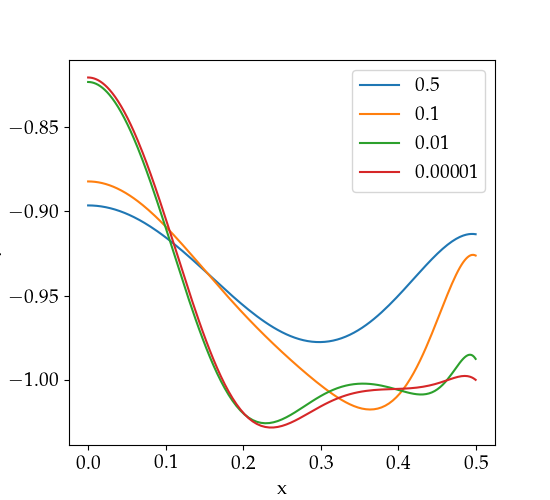
Figure 2 shows that regularization spreads the current density across the island, and figure 3 shows the 2D structure of the island. Clearly $J\neq J(\psi)$, so our theory of island growth must account for the structure of the current. The shape factor $g_{1}$ incorporates this structure. Rather than a constant $g_{1}\simeq 0.8$, evaluating $g_{1}$ as a time-dependent quantity results in significantly slowed island growth. The details of the modified Rutherford model derivation, including the dimensionless integrals that give $g_{1}$, $c_{\mu}$, and $c_{\nu}$, are given in Appendix B.

Preliminary investigation of reconnection in Voigt-MHD found that, when resistivity is included, the saturated state was independent of the regularization and dissipation parameters [10]. The model presented here explains this observation; at steady state, equation (30) is independent of these parameters. Figure 4 is one of many examples; for all parameter values tested with $\delta=0.1$, the same saturated island width is found. Moreover, if the final state is independent of the regularization parameters, the island width must be that predicted by ideal theory. Recalling that $L_{x}=a/2$, the outer layer first described by Hahm and Kulsrud has an island of width

$$w=\sqrt{\frac{2a\delta}{\cosh(ka/2)}}.$$ (32)

Figure 5 demonstrates excellent agreement between the ideal prediction and the saturated Voigt island widths. The island growth and saturation for $\delta=10^{-2}$ and $10^{-3}$ appears to be monotonic, as predicted by a Rutherford-like model. However, for $\delta=0.03$ the island width evolves as an underdamped oscillator. The modified Rutherford model does not capture these transient dynamics. Figure 6 shows that, for the case $\delta=10^{-3}$, the modified Rutherford model is a better predictor of $\frac{dw}{dt}$ than the standard Rutherford model (which holds $g_{1}$ constant), but our model overestimates the strength of the Voigt braking effect. These shortcomings of the modified Rutherford model will be addressed in future work.

Figure 5: Island width evolution for cases (a) $\delta=0.03,L_{y}=7$; (b) $\delta=0.01,L_{y}=1.5$; and (c) $\delta=10^{-3},L_{y}=3.5$.

Figure 6: Standard Rutherford model with $g_{1}=0.823$, and modified ($g_{1}=g_{1}(t)$) Rutherford island growth with and without Voigt braking compared to numerical results for the case $L_{y}=3.5,\delta=10^{-3}$.

V Equilibrium

In this section we consider the long-time behavior of the Voigt system with dissipation and present evidence that the theorem of Constantin and Pasqualotto [2] which guarantees convergence to an ideal equilibrium may be generalized to this case. The system (2)–(5) conserves a modified energy[10] (which may be identified with the usual norm on the Sobolev space $H^{1}$)

$$\frac{1}{2}\frac{d}{dt}\int d^{3}x\left(B^{2}+\alpha_{2}J^{2}+u^{2}+\alpha_{1}\omega^{2}\right)=$$ (33)

$$-\int d^{3}x\left(\nu\omega^{2}+\eta J^{2}+\frac{\mu}{2}u^{2}\right)-\int d^{3}x\boldsymbol{E}_{\text{ext}}\cdot\boldsymbol{J},$$ (34)

where the vorticity $\boldsymbol{\omega}=\nabla\times\boldsymbol{u}$. In particular, when the applied field vanishes, this energy is monotonically decaying in time. Nonzero $\alpha_{2}$ grants control on the $L_{2}$ norm of $J$, prohibiting the formation of $\delta$-function current sheets. The additional friction term adds a sign-definite dissipation on the RHS of equation (34), so we do not anticipate worsened regularity from $\mu\neq 0$. In steady state with nonzero $\eta$, equation (3) gives a residual flow

$$\boldsymbol{u}\times\boldsymbol{B}=\eta\boldsymbol{J}+\boldsymbol{E}_{ext}.$$ (35)

When $\mu$ vanishes, steady-state momentum balance reads

$$\boldsymbol{J}\times\boldsymbol{B}=\nabla p-\nu\nabla^{2}\boldsymbol{u}+\boldsymbol{u}\cdot\nabla\boldsymbol{u}.$$ (36)

The deviation from ideal MHS equilibrium $\boldsymbol{J}\times\boldsymbol{B}=\nabla p$ is an undesirable complication in the context of 3D equilibrium computation. On the other hand, the theorems of Constantin and Pasqualotto [2, 14] guarantee ( when $\mu=\eta=0$, $\boldsymbol{E}_{ext}=0$, and for sufficiently regular initial conditions) an asymptotic state of the system (2)–(5) that exactly satisfies the ideal MHS equilibrium relation. By including $\mu\neq 0$ in addition to $\eta$ and $\boldsymbol{E}_{ext}$, equation (34) suggests that a steady state may only be attained if the flow is entirely dissipated, recovering $\boldsymbol{J}\times\boldsymbol{B}=\nabla p$. A proof of this result is beyond the scope of this work, but we state it here as a conjecture and give numerical evidence in support.

In figure 7, the strong decay of the kinetic energy $\int u^{2}$ induced by large values of $\nu$ and $\mu$ is evident. Figure 8 shows the volume-averaged force residual $|\boldsymbol{J}\times\boldsymbol{B}-\nabla p|$, which rapidly decays to machine-precision zero in the case $\mu=0.5$, indicating that the ideal MHS equilibrium condition is satisfied, and that there is some speed-up in convergence compared to cases without friction. We also note that the form of the applied field implies that, when the flow has entirely dissipated, the final current must equal the initial current. Therefore, the addition of friction restricts the final equilibrium to differ from the initial state by only a vacuum magnetic field.

The numerical results presented in this study suggest that the Voigt-regularized MHD equations behave as a strongly damped system where the magnetic topology is constrained by a competition between the inductive scale $\alpha$ and the dissipative scales $\eta$ and $\nu$. While the Constantin-Pasqualotto theorems provide a rigorous foundation for the existence and uniqueness of solutions in 2D MHD, our findings indicate that the inclusion of the Voigt-brake $\mathcal{B}$ fundamentally alters the nonlinear saturation manifold.

Figure 7: Kinetic energy decay for $\delta=0.1$ and $\alpha_{1}=\alpha_{2}=0.5$ with $\mu=\nu=0.5,0.1,0.01$ and $10^{-3}$ and $\mu=0$, $\nu=10^{-3}$ with timestep 30.

Figure 8: Volume-averaged force residual decay for $\delta=0.1$ and $\alpha_{1}=\alpha_{2}=0.5$ with $\mu=\nu=0.5,0.1,0.01$ and $10^{-3}$ and $\mu=0$, $\nu=10^{-3}$ with timestep 30.

VI Conclusion

Our investigation of Voigt-regularized MHD has uncovered several key insights: In section III, we saw that the linear phase of forced reconnection is rapid compared to resistive MHD, forgoing the need for a singular current sheet to develop. In section IV, we found that the island evolution has subtle deviations from a Rutherford-like model, but the saturated width is insensitive to the choice of regularization and dissipation parameters. Finally, in section V we presented the first evidence that Voigt-regularized MHD with friction can generate precise MHS equilibria without flows - and, we reiterate, that the choice of regularization parameters does not meaningfully affect the final equilibrium state.

It remains an open question how these phenomena will be complicated by the effects of reactor-relevant geometry. The highly shaped, 3D magnetic fields of optimized stellarators will undoubtedly present many challenges, which we hope to address in future work.

Appendix A Voigt Helicity and Electron Inertia

There is an intriguing similarity between the induction equation (3) and that of inertial MHD, as studied in Hamiltonian reconnection [6]. There one finds

$$\partial_{t}\left(\boldsymbol{B}-d_{e}^{2}\nabla^{2}\boldsymbol{B}\right)=\nabla\times\left(\boldsymbol{u}\times\left(\boldsymbol{B}-d_{e}^{2}\nabla^{2}\boldsymbol{B}\right)\right).$$ (37)

The electron skin depth $d_{e}$ plays a similar role to the Voigt regularization length $\alpha_{2}^{1/2}$. However, inertial MHD has a noncanonical Hamiltonian structure[13] that is apparent in that $d_{e}$ appears on both sides of the induction equation, so $\boldsymbol{B}-d_{e}^{2}\nabla^{2}\boldsymbol{B}$ is dual to an advected one-form with associated conserved helicity

$$\mathcal{K}_{e}=\int d^{3}x\left(\boldsymbol{A}-d_{e}^{2}\nabla^{2}\boldsymbol{A}\right)\cdot\left(\boldsymbol{B}-d_{e}^{2}\nabla^{2}\boldsymbol{B}\right),$$ (38)

which effectively counts linkages of a field $\tilde{\boldsymbol{B}}\equiv\boldsymbol{B}-d_{e}^{2}\nabla^{2}\boldsymbol{B}$. The Voigt MHD induction equation does not respect such a variational structure. Nevertheless, as proved by Constantin and Pasqualotto[2], it does conserve a “helicity"

$$\mathcal{K}=\int d^{3}x\boldsymbol{B}\cdot\left(\boldsymbol{A}-\alpha_{2}\nabla^{2}\boldsymbol{A}\right),$$ (39)

which we recognize as the weighted sum of the familiar magnetic helicity $\int\boldsymbol{A}\cdot\boldsymbol{B}$ and the current helicity $\int\boldsymbol{B}\cdot\boldsymbol{J}$. In other words, Voigt MHD allows change in magnetic topology, but only when the topology of current lines changes to compensate.

Appendix B Derivation of the Voigt-Regularized Nonlinear Island Evolution Equation

We consider a 2D slab geometry with magnetic shear $B^{\prime}_{y}$. The helical flux function $\Psi$ near the resonant surface $x=0$ is defined as:

$$\Psi(x,y,t)=\frac{1}{2}B^{\prime}_{y}x^{2}+\psi_{s}(t)\cos(ky).$$ (40)

where $\psi_{s}(t)$ is the reconnected flux at the O-point. The island full-width $w$ is defined by the separatrix $\Psi=\psi_{s}$, yielding:

$$w=4\sqrt{\frac{\psi_{s}}{B^{\prime}_{y}k}}.$$ (41)

The flux-surface average $\langle F\rangle$ of a quantity $F$ is defined by integrating along a surface of constant $\Psi$:

$$\langle F\rangle=\frac{\oint\frac{F}{\partial_{x}\Psi}dy}{\oint\frac{1}{\partial_{x}\Psi}dy}=\frac{\oint\frac{F}{\sqrt{\Psi-\psi_{s}\cos ky}}dy}{\oint\frac{1}{\sqrt{\Psi-\psi_{s}\cos ky}}dy}.$$ (42)

The longitudinal component of Ohm’s Law in the presence of Voigt regularization ($\alpha_{2}$) is:

$$\left\langle\frac{\partial\psi}{\partial t}-\alpha_{2}\nabla^{2}\frac{\partial\psi}{\partial t}\right\rangle=\eta\langle j\rangle+E_{ext}.$$ (43)

Integrating across the island width and applying the flux-surface average removes the convective term $\boldsymbol{v}\cdot\nabla\psi$. Substituting $j\approx\partial_{x}^{2}\psi$ and differentiating $w(t)$ yields the modified Rutherford equation:

$$(1+\mathcal{B})g_{1}\frac{dw}{dt}=\eta\Delta^{\prime}(w)$$ (44)

where $g_{1}$ is the shape factor and $\mathcal{B}$ is the dimensionless Voigt-inertial brake, discussed below.

The shape factor $g_{1}$ is defined as the following dimensionless double integral over the island interior:

$$g_{1}=\frac{1}{\sqrt{2}\pi}\int_{-1}^{1}\frac{\langle\cos(ky)\rangle^{2}}{\langle 1\rangle}d\Omega.$$ (45)

Expanding the averages explicitly:

$$g_{1}=\frac{1}{\sqrt{2}\pi}\int_{-1}^{1}\frac{\left(\int_{0}^{\theta_{max}}\frac{\cos\theta d\theta}{\sqrt{\Omega+\cos\theta}}\right)^{2}}{\int_{0}^{\theta_{max}}\frac{d\theta}{\sqrt{\Omega+\cos\theta}}}d\Omega.$$ (46)

The integrals over $\theta$ are expressed using complete elliptic integrals of the first ($K$) and second ($E$) kind. Defining the modulus $m=\frac{2}{\Omega+1}$, the averaged terms are:

$$\langle 1\rangle=\sqrt{m}K(m),\quad\langle\cos\theta\rangle=\sqrt{m}[2E(m)-K(m)].$$ (47)

Substituting these into the expression for $g_{1}$:

$$g_{1}=\frac{2}{\pi}\int_{0}^{1}\left(\frac{2E(m)}{K(m)}-1\right)^{2}K(m)\,dm.$$ (48)

Numerical integration over the modulus $m$ from the O-point to the separatrix yields:

$$g_{1}\approx 0.823.$$ (49)

The factor $\mathcal{B}$ represents the total inertial and viscous resistance provided by the regularization:

$$\mathcal{B}=\frac{1}{\eta}\left(c_{\mu}\alpha_{1}\mu+c_{\nu}\nu\right).$$ (50)

To understand the origin of $c_{\mu}$ and $c_{\nu}$, we must examine the flow field (velocity) created by a growing island. In a growing island, the magnetic flux $\psi_{s}$ increases over time. Because the plasma is frozen into the magnetic field (outside the small resistive region), the plasma must move to accommodate this new flux. The velocity field $\boldsymbol{v}$ is not arbitrary, but strictly coupled to the growth of the island width $w$. Mathematically, this is expressed by the stream function $\phi$:

$$\phi(x,y,t)=\dot{w}\cdot\Phi(x,y),$$ (51)

where $\dot{w}=\frac{dw}{dt}$ is the growth rate and $\Phi(x,y)$ is the spatial flow template. If the island grows faster ($\dot{w}$ is large), the plasma must be pushed out of the way faster. This creates a direct link between the kinetic energy and viscous disspation and the rate of change of the island width. When we plug this into the momentum equation and integrate across the island, we obtain a force-balance condition whereby the magnetic drive ($\Delta^{\prime}$) is on one side, and terms proportional to $\dot{w}$ are on the other. The constants $c_{\mu}$ and $c_{\nu}$ are the resulting coefficients of proportionality.

As the island grows, it pushes plasma from the X-points toward the O-point and then out along the separatrix. This creates vortices (flow cells). Viscosity ($\nu$) resists this motion. The coefficient $c_{\nu}$ comes from calculating the total viscous dissipation power $P_{\nu}$:

$$P_{\nu}=\iint\nu|\nabla^{2}\phi|^{2}\,dx\,dy.$$ (52)

By substituting $\phi=\dot{w}\Phi$, we pull $\dot{w}$ out of the integral:

$$P_{\nu}=\nu\dot{w}^{2}\left[\iint|\nabla^{2}\Phi|^{2}\,dx\,dy\right].$$ (53)

The term in the brackets, normalized by the magnetic parameters, is exactly $c_{\nu}$. The value $1.35$ specifically accounts for the fact that the flow is not just inside the island, but extends into the “outer” region, where the vortices decay spatially.

The Voigt regularization adds a term $\alpha_{1}\nabla^{2}\partial_{t}\boldsymbol{u}$. Physically, this acts like extra inertia, just as $\alpha_{2}$ plays a role similar to electron mass (see Appendix A). It resists the acceleration of the plasma as the island opens. The coefficient $c_{\mu}$ comes from the integral of the gradient of the flow:

$$W_{\alpha}=\iint\alpha_{1}|\nabla\dot{\phi}|^{2}\,dx\,dy.$$ (54)

This integral represents the work done against the inductive-inertial “drag” of the Voigt model. The value $0.35$ is smaller than $c_{\nu}$ because the Voigt term involves fewer spatial derivatives than the viscous term (which is a bi-harmonic $\nabla^{4}$ operator). The Voigt term is more concentrated near the reconnection layer, whereas viscosity “feels” the entire volume of the island vortices.

When we combine these, the Rutherford equation changes to:

$$\underbrace{\eta\Delta^{\prime}}_{\text{Magnetic Drive}}=\underbrace{g_{1}\dot{w}}_{\text{Standard Resistive Drag}}+\underbrace{g_{1}\mathcal{B}\dot{w}}_{\text{Voigt + Viscous Brake}}.$$ (55)

Here the brake term $\mathcal{B}$ is:

$$\mathcal{B}=\frac{1}{\eta}\left(\smash{\underbrace{c_{\mu}\alpha_{1}\mu}_{\text{Inductive}}+\underbrace{c_{\nu}\nu}_{\text{Viscous}}}\right).$$ (56)

References

- [1] (1997-11) Implicit-explicit runge-kutta methods for time-dependent partial differential equations. Applied Numerical Mathematics 25 (2-3), pp. 151–167. External Links: Document Cited by: §II.
- [2] (2023-06) Magnetic relaxation of a voigtâĂŞmhd system. Communications in Mathematical Physics 402 (2), pp. 1931–1952. External Links: Document, ISSN 1432-0916 Cited by: Appendix A, §I, §V, §V.
- [3] (2020-10) DESC: a stellarator equilibrium solver. Physics of Plasmas 27 (10), pp. 102513. External Links: Document Cited by: §I.
- [4] (1987) Ideal magnetohydrodynamics. Plenum Press, New York. Cited by: §I.
- [5] (1967) Toroidal containment of a plasma. Phys. Fluids 10 (1), pp. 137–154. Cited by: §I.
- [6] (1999) Hamiltonian magnetic reconnection. Plasma Physics and Controlled Fusion 41 (12), pp. 1497. Cited by: Appendix A, §II.
- [7] (1985) Forced magnetic reconnection. Phys. Fluids 28 (8), pp. 2412–2418. Cited by: §II.
- [8] (2011-06) SIESTA: a scalable iterative equilibrium solver for toroidal applications. Physics of Plasmas 18 (6). External Links: Document, ISSN 1089-7674 Cited by: §I.
- [9] (1983) Steepest-descent moment method for three-dimensional magnetohydrodynamic equilibria. Physics of Fluids 26 (12), pp. 3553. External Links: Document Cited by: §I.
- [10] (2025-06) Computation of magnetohydrodynamic equilibria with voigt regularization. Physics of Plasmas 32 (6), pp. 062507. External Links: ISSN 1070-664X, Document, Link, https://pubs.aip.org/aip/pop/article-pdf/doi/10.1063/5.0267510/20563856/062507_1_5.0267510.pdf Cited by: §I, §I, §II, §IV, §V, footnote 1.
- [11] (2012-11) Computation of multi-region relaxed magnetohydrodynamic equilibria. Physics of Plasmas 19 (11), pp. 112502. External Links: Document Cited by: §I.
- [12] (2025) An introduction to stellarators: from magnetic fields to symmetries and optimization. Society for Industrial and Applied Mathematics (SIAM), Philadelphia, PA. External Links: Document, ISBN 978-1-61197-821-6 Cited by: §I, §I.
- [13] (1984-04) Hamiltonian formulation of reduced magnetohydrodynamics. The Physics of Fluids 27 (4), pp. 886–897. External Links: ISSN 0031-9171, Document, Link, https://pubs.aip.org/aip/pfl/article-pdf/27/4/886/12518533/886_1_online.pdf Cited by: Appendix A.
- [14] (2021) Nonlinear waves in general relativity and fluid dynamics. Ph.D. Thesis, Princeton University. Cited by: §V.
- [15] (2002) Numerical recipes in c++: the art of scientific computing. second edition, Cambridge University Press. Cited by: §I.
- [16] (2017-03) HINT modeling of three-dimensional tokamaks with resonant magnetic perturbation. Plasma Physics and Controlled Fusion 59 (5), pp. 054008. External Links: Document, ISSN 1361-6587 Cited by: §I.
- [17] (1974) Relaxation of toroidal plasma and generation of reverse magnetic fields. Phys. Rev. Lett. 33 (19), pp. 1139–1141. Cited by: §I.