Reparameterized Tensor Ring Functional Decomposition for Multi-Dimensional Data Recovery

Abstract

Tensor Ring (TR) decomposition is a powerful tool for high-order data modeling, but is inherently restricted to discrete forms defined on fixed meshgrids. In this work, we propose a TR functional decomposition for both meshgrid and non-meshgrid data, where factors are parameterized by Implicit Neural Representations (INRs). However, optimizing this continuous framework to capture fine-scale details is intrinsically difficult. Through a frequency-domain analysis, we demonstrate that the spectral structure of TR factors determines the frequency composition of the reconstructed tensor and limits the high-frequency modeling capacity. To mitigate this, we propose a reparameterized TR functional decomposition, in which each TR factor is a structured combination of a learnable latent tensor and a fixed basis. This reparameterization is theoretically shown to improve the training dynamics of TR factor learning. We further derive a principled initialization scheme for the fixed basis and prove the Lipschitz continuity of our proposed model. Extensive experiments on image inpainting, denoising, super-resolution, and point cloud recovery demonstrate that our method achieves consistently superior performance over existing approaches. Code is available at https://github.com/YangyangXu2002/RepTRFD.

1 Introduction

Low-rank tensor representations have become a fundamental tool for modeling multi-dimensional data across a wide range of computer vision and signal processing tasks, such as image and video processing [19, 20], remote sensing [10, 5], medical imaging [24], and data compression [13, 6]. By exploiting the underlying low-dimensional structures, classical tensor decompositions such as CANDECOMP/PARAFAC (CP) [4, 11], Tucker [39, 7], Tensor Train (TT) [27], and Tensor Ring (TR) [46] provide compact representations and facilitate recovery from incomplete or corrupted data.

Figure 1: (a) Frequency analysis of TR factors. Low-pass filtering $\{\mathcal{G}^{(k)}\}_{k=1}^{3}$ along mode-2 yields the low-frequency counterparts $\{\tilde{\mathcal{G}}^{(k)}\}_{k=1}^{3}$. Reconstructing via the contraction $\Phi(\cdot)$ using these factors shows noticeable attenuation along the corresponding modes. (b) Qualitative comparison of TRLRF [45], TRFD, and RepTRFD for meshgrid and non-meshgrid data recovery. Compared with TRLRF, our methods (TRFD and RepTRFD) effectively handle non-meshgrid data and demonstrate marked improvements over the baseline.

Among these, TR decomposition has been widely studied for its ability to efficiently represent high-order tensors with compact structures [42, 45, 28, 16]. However, traditional TR formulations are inherently discrete and assume that data are defined on fixed grids, which limits their applicability to continuous signals and resolution-independent modeling. To address the limitation in discrete tensor decomposition, a general framework known as low-rank tensor functional representation has been proposed [21]. In this paradigm, tensor factors are modeled as Implicit Neural Representations (INRs) [37] that map continuous coordinates to latent factor values, effectively placing tensor decomposition in a continuous functional space. While this functional framework has been successfully extended to various decomposition formats [41, 40, 14] and improved with continuous regularizations [22, 23], extending TR decomposition to this continuous setting remains unexplored.

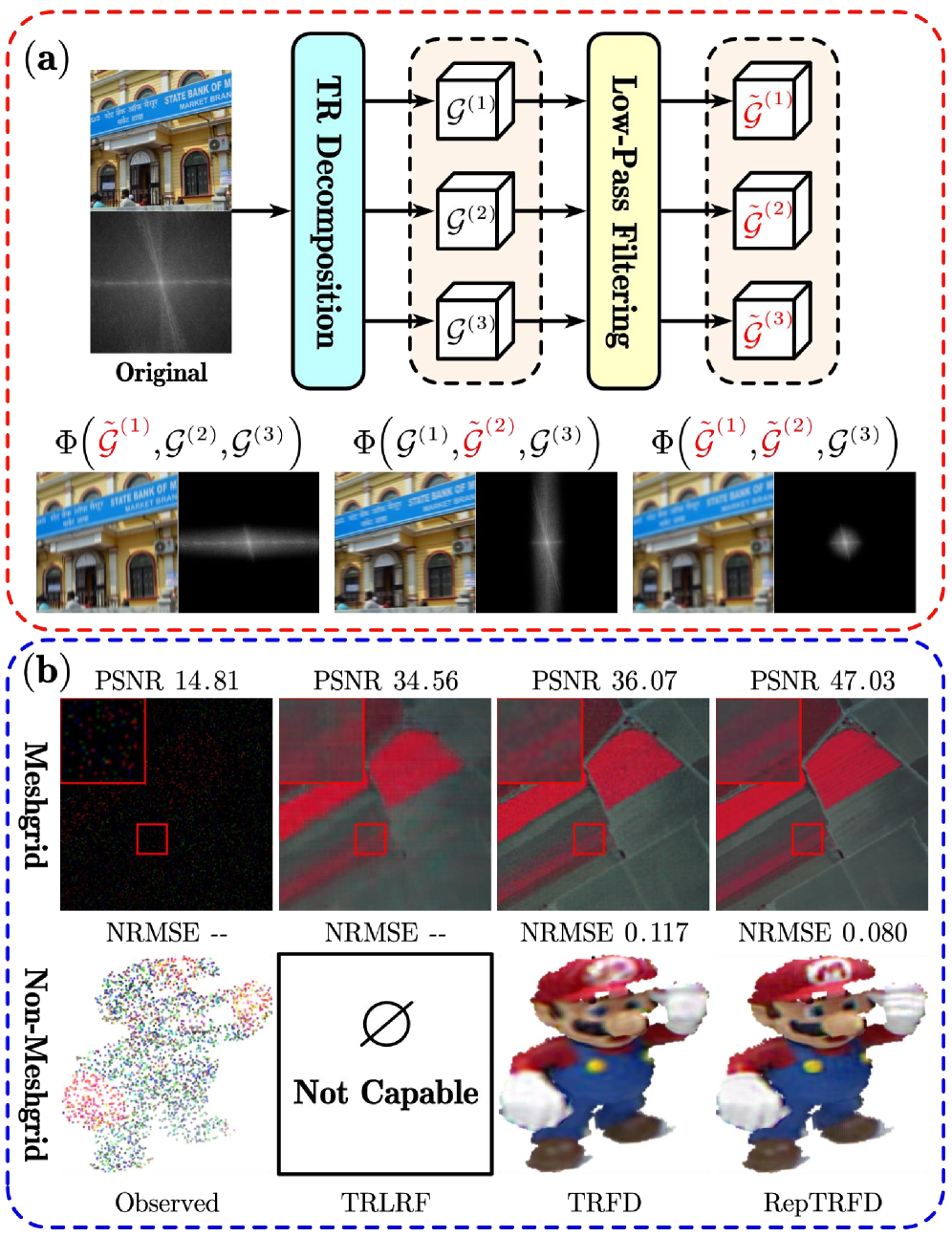
Inspired by existing functional tensor methods, we propose a TR Functional Decomposition (TRFD) for multidimensional image recovery. It is worth noting that establishing this decomposition is non-trivial due to the intrinsic properties of TR factors, and direct application of existing functional tensor methods often produces reconstructions dominated by low-frequency components. To further understand this limitation, we analyze TR decomposition from a frequency perspective. As illustrated in Fig. 1, replacing the original TR factors $\{\mathcal{G}^{(k)}\}_{k=1}^{3}$ with their low-pass filtered versions $\{\tilde{\mathcal{G}}^{(k)}\}_{k=1}^{3}$ yields reconstructions that exhibit noticeable attenuation along the corresponding modes. This finding reveals that the frequency characteristics of TR factors are directly inherited by the reconstructed tensor.

However, due to the inherent spectral bias of INRs [29], learning TR factors that capture appropriate high-frequency components remains highly challenging. Distinct from existing approaches, we take a novel perspective by revisiting the factor learning process through the lens of training dynamics. Specifically, we seek to transform the parameter space of the TR factors, so that the optimization dynamics can more effectively explore high-frequency directions. To achieve this, we propose Reparameterized TRFD (RepTRFD), in which each TR factor is expressed as a structured combination of a learnable latent tensor and a fixed basis. This reparameterization is theoretically shown to enhance the training dynamics, allowing the TR structure to fully exploit both meshgrid and continuous data. As illustrated in Fig. 1, it significantly improves the reconstruction of high-frequency details. By incorporating this, we offer a novel perspective for advancing the study of tensor functional representations. In summary, our main contributions are as follows:

• We extend the TR decomposition to the continuous domain and provide a frequency-domain analysis of the challenge in learning TR factors that capture high-frequency components.

• We propose a reparameterization strategy for TR factors, where each factor is expressed as a structured combination of a learnable tensor and a fixed basis, which facilitates the learning of high-frequency details.

• We theoretically show that this reparameterization enhances the training dynamics, and further derive a principled initialization scheme while providing the Lipschitz continuity guarantees. Extensive experiments demonstrate the superiority of our approach.

2 Related Work

Implicit Neural Representations. INRs have recently emerged as a powerful paradigm for representing continuous signals by mapping coordinates to values [37]. Subsequent works have sought to enhance the representational power and efficiency of INRs through improved activation functions [30, 34, 17], encoding schemes [38, 25], and training dynamics [3, 36]. Despite their expressive power, learning global mappings over entire signals still exhibits limited computational efficiency, and the lack of structural priors often limits performance in inverse problems.

Tensor Functional Representations. Recent works have extended low-rank tensor representations to the continuous domain. Unlike INRs that map coordinates to the entire signal, these methods learn coordinate-to-factor mappings, enabling continuous modeling with lower computational cost and inherent low-rank priors. Representative approaches include the low-rank tensor function representation (LRTFR) [21] based on Tucker decomposition, a functional transform-based factorization [41] that improves expressiveness, a parameter-efficient deep rank-one factorization (DRO-TFF) [14] that reduces storage and computation overhead, and unified functional extensions of CP and TT decompositions [40]. Moreover, these functional tensor formulations can be synergistically combined with continuous regularization methods, such as neural total variation (NeurTV) [23] and continuous representation-based nonlocal (CRNL) [22] priors, to further enhance reconstruction quality and structural consistency.

Reparameterization and Training Dynamics. Reparameterization techniques have been widely adopted in deep learning to improve training dynamics. Early work by Salimans et al. [31] first stabilized optimization by decoupling the magnitude and direction of weights through weight normalization. Following this, Ding et al. [8] further extended it to structural reparameterization with parallel branches. Mostafa [26] explored another perspective by decoupling weight optimization from sparse connectivity learning. More recently, Shi et al. [36] factorized network weights into a learnable matrix and a fixed Fourier basis, enhancing learning behavior in INRs. In addition, several works have explored alternative approaches to improving the training dynamics of INRs and achieved promising results [3, 15, 35]. In this work, we take the first step toward analyzing low-rank tensor functional representations through training dynamics, highlighting the potential of reparameterization for more effective factor learning.

3 Methodology

3.1 Notations and Preliminaries

To enhance readability, we denote scalars by lowercase letters (e.g., $x$), vectors by bold lowercase (e.g., $\mathbf{x}$), matrices by bold uppercase (e.g., $\mathbf{X}$), and tensors by calligraphic letters (e.g., $\mathcal{X}$). Given a $d$-th order tensor $\mathcal{X}\in\mathbb{R}^{n_{1}\times n_{2}\times\cdots\times n_{d}}$, its $\mathbf{v}$-th entry is written as $\mathcal{X}_{\mathbf{v}}$ where $\mathbf{v}=[v_{1},v_{2},\dots,v_{d}]^{\mathrm{T}}$. We also define the mode-$k$ slice at index $v_{k}$ as $\mathcal{X}_{:v_{k}:}\in\mathbb{R}^{n_{1}\times\cdots\times n_{k-1}\times n_{k+1}\times\cdots\times n_{d}}$. In addition, $\|\mathcal{X}\|_{\infty}$ is the infinity norm of $\mathcal{X}$ by calculating the maximum magnitude of the tensor’s entries. We next introduce two fundamental definitions used throughout this paper.

Definition 1 (Tensor Ring Decomposition [46]).

Consider a $d$-th order tensor $\mathcal{X}\in\mathbb{R}^{n_{1}\times n_{2}\times\cdots\times n_{d}}$, TR decomposition represents $\mathcal{X}$ using third-order cores $\mathcal{G}^{(k)}\in\mathbb{R}^{r_{k}\times n_{k}\times r_{k+1}}$ for $k=1,2,\dots,d$, with the circular constraint $r_{d+1}=r_{1}$. The tuple $[r_{1},r_{2},\dots,r_{d}]$ is referred to as the TR rank, which controls the representation capacity. Each element of $\mathcal{X}$ is given by

$$\mathcal{X}_{\mathbf{v}}=\operatorname{trace}\left(\mathcal{G}^{(1)}_{:v_{1}:}\mathcal{G}^{(2)}_{:v_{2}:}\cdots\mathcal{G}^{(d)}_{:v_{d}:}\right),$$ (1)

where $\operatorname{trace}(\cdot)$ denotes the matrix trace. For simplicity, the decomposition is presented as

$$\mathcal{X}=\Phi(\mathcal{G}^{(1)},\mathcal{G}^{(2)},\dots,\mathcal{G}^{(d)}),$$ (2)

where $\Phi(\cdot)$ denotes the TR contraction operation.

Definition 2 (Mode-$k$ Discrete Fourier Transform [13, 18]).

Given a $d$-th order tensor $\mathcal{X}\in\mathbb{R}^{n_{1}\times n_{2}\times\cdots\times n_{d}}$, its mode-$k$ Discrete Fourier Transform (DFT) is defined as

$$\mathscr{F}_{k}[\mathcal{X}]=\mathcal{X}\times_{k}\mathbf{F}_{k},$$ (3)

where $\mathbf{F}_{k}\in\mathbb{C}^{n_{k}\times n_{k}}$ is the DFT matrix, and $\times_{k}$ is the $k$-mode product between tensor and matrix.

3.2 Tensor Ring Functional Decomposition

Traditional TR decomposition assumes that each factor $\mathcal{G}^{(k)}$ is a discrete tensor defined on a fixed grid. To extend the discrete TR model into a continuous representation, we reinterpret each TR factor as a functional tensor parameterized by INRs. Since the TR factors are inherently linked through cyclic contractions, we introduce a shared frequency embedding to enhance their consistency across modes.

Figure 2: Illustration of proposed TRFD and RepTRFD. TRFD directly learns a continuous mapping from coordinates to TR factors. In contrast, RepTRFD reparameterizes each TR factor as a structured combination of a learnable latent tensor and a fixed basis, which improves the training dynamics and facilitates more effective learning of high-frequency components.

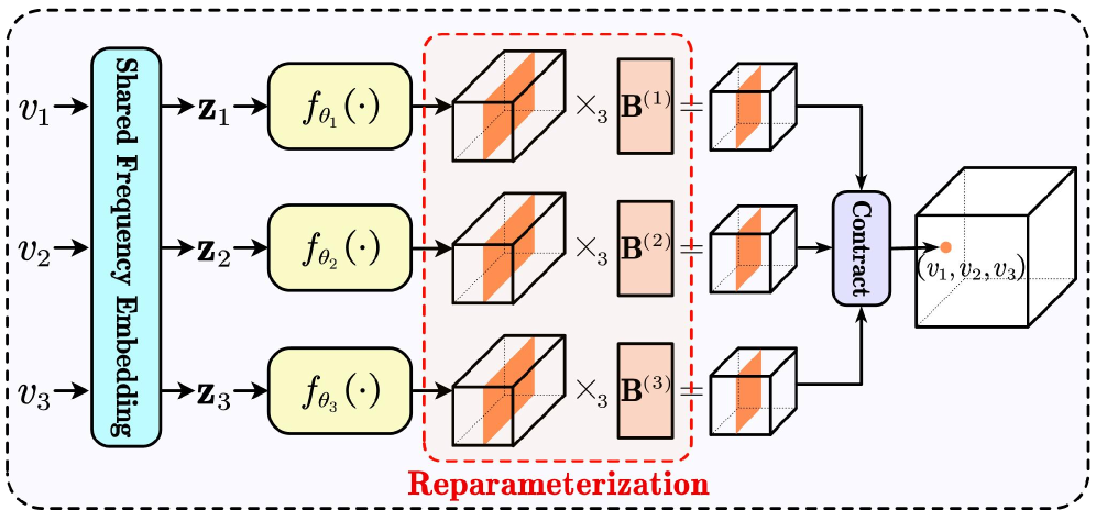
As illustrated in Fig. 2, given a coordinate vector $\mathbf{v}=[v_{1},v_{2},\dots,v_{d}]^{\mathrm{T}}$, the shared embedding for the $k$-th dimension is implemented by a single sinusoidal layer:

$$\mathbf{z}_{k}=\sin(\omega_{0}(\mathbf{w}v_{k}+\mathbf{b}))\in\mathbb{R}^{h},\quad k=1,\dots,d,$$ (4)

where $\omega_{0}$ is a frequency scaling parameter, $\mathbf{w}\in\mathbb{R}^{h}$ and $\mathbf{b}\in\mathbb{R}^{h}$ are learnable weight and bias, and $h$ denotes the hidden dimension of the sinusoidal layer. To generate each TR factor, we employ a separate branch network for each mode. Each branch is a multi-layer perceptron (MLP) that maps the corresponding embedding $\mathbf{z}_{k}$ to a vector of length $r_{k}r_{k+1}$, which is then reshaped into the desired TR slice:

$$\mathcal{G}^{(k)}_{:v_{k}:}=f_{\theta_{k}}(\mathbf{z}_{k})=g_{\theta_{k}}(v_{k})\in\mathbb{R}^{r_{k}\times r_{k+1}},v_{k}\in\{1,\dots,n_{k}\},$$ (5)

where $f_{\theta_{k}}(\cdot)$ denotes the MLP associated with the $k$-th tensor mode, producing the mode-specific factor slice from the shared embedding, and $g_{\theta_{k}}(\cdot)$ is the function composed with MLP and shared frequency embedding. This approach naturally extends the TR decomposition to a continuous representation, which we refer to as the Tensor Ring Functional Decomposition (TRFD).

3.3 Reparameterization for Factor Learning

Frequency Analysis of TR Factors. While the TR functional decomposition provides a flexible and compact framework for representing high-dimensional data, its practical effectiveness is often constrained by the inherent spectral bias of the INRs used to parameterize the factors. INRs tend to prioritize low-frequency components while underrepresenting high-frequency details, leading to limited expressiveness within the individual TR factors. Crucially, this spectral limitation does not remain confined to the factor level, because it propagates through the cyclic contractions of the TR structure and influences the frequency characteristics of the reconstructed tensor $\mathcal{X}$. To better understand this phenomenon, we formally analyze how the frequency content of the TR factors propagates through the reconstruction process. The following theorem presents the corresponding characterization.

Theorem 1.

Let $\mathcal{X}=\Phi(\mathcal{G}^{(1)},\dots,\mathcal{G}^{(d)})$ be a TR decomposition. Suppose that the mode-2 frequency components of $\mathcal{G}^{(k)}$ beyond a threshold $\Omega_{k}$ are negligible for all $k$, i.e.,

$$\|\big(\mathscr{F}_{2}[\mathcal{G}^{(k)}]\big)_{:\omega_{k}:}\|_{\infty}\leq\epsilon,\ \forall|\omega_{k}|>\Omega_{k},k=1,2,\dots,d,$$

where $\epsilon>0$ is a small constant. Then the reconstructed tensor $\mathcal{X}$ also exhibits attenuated high-frequency content along mode $k$:

$$\|\big(\mathscr{F}_{k}[\mathcal{X}]\big)_{:\omega_{k}:}\|_{\infty}\leq c_{k}\,\epsilon,\ \forall|\omega_{k}|>\Omega_{k},k=1,2,\dots,d,$$

where $c_{k}$ is a constant depending only on the magnitudes of the remaining cores $\{\mathcal{G}^{(j)}\}_{j\neq k}$.

All proofs of the theoretical results presented in this section are provided in the supplementary material. Theorem 1 indicates that the spectral content of each TR factor directly affects the corresponding dimension of the reconstructed tensor. Consequently, achieving accurate reconstruction of high-frequency tensors is contingent on the TR factors themselves containing sufficiently high-frequency components. However, due to the inherent spectral bias of standard INRs, learning such factors is challenging. This motivates the design of strategies that facilitate the acquisition of high-frequency information.

Reparameterized Tensor Ring. To address this challenge, we aim to transform the parameter space of the TR factors to improve the training dynamics, thereby facilitating more efficient learning of the TR factors. Specifically, by introducing a fixed basis $\mathbf{B}^{(k)}\in\mathbb{R}^{r_{k+1}\times R_{k+1}}$, we reparameterize each TR factor as a combination of a learnable latent tensor and this basis, which is expressed as

$$\mathcal{G}^{(k)}=\mathcal{C}^{(k)}\times_{3}\mathbf{B}^{(k)},\quad k=1,\ldots,d.$$ (6)

This decomposition separates the learnable component from the fixed basis, allowing each TR factor to be expressed as a structured combination of latent elements. Such a formulation improves the conditioning of the optimization and facilitates more effective learning of high-frequency components, as shown in the following theorem.

Theorem 2.

Consider a TR factor $\mathcal{G}$ reparameterized as $\mathcal{G}=\mathcal{C}\times_{3}\mathbf{B}$, where $\mathcal{C}\in\mathbb{R}^{r_{1}\times n\times R_{2}}$ is a trainable tensor and $\mathbf{B}\in\mathbb{R}^{r_{2}\times R_{2}}$ is a fixed basis. Let $\mathsf{L}(\omega)$ be the loss associated with frequency $\omega$. For any $\omega_{\rm high}>\omega_{\rm low}>0$, given any $\epsilon\geq 0$, and fixed indices $p,q$ with $1\leq p\leq r_{1}$ and $1\leq q\leq n$, there exists a matrix $\mathbf{B}$ such that for all $s=1,\dots,R_{2}$,

Theorem 2 demonstrates that our reparameterization amplifies the gradient response to high-frequency components relative to low-frequency ones. This implies that the optimization becomes more responsive to fine-scale variations, effectively improving the convergence behavior when learning TR factors with rich spectral content. To realize these benefits in practice, we need to specify how to determine the latent tensor $\mathcal{C}^{(k)}$ and fixed basis $\mathbf{B}^{(k)}$.

Similar to TRFD, we represent the latent tensor $\mathcal{C}^{(k)}$ as generated slice by slice through a neural mapping. Specifically, given a coordinate $v_{k}$, the corresponding slice $\mathcal{C}^{(k)}_{:v_{k}:}$ is produced by applying a shared frequency embedding and an MLP as:

$$\mathcal{C}^{(k)}_{:v_{k}:}=g_{\theta_{k}}(v_{k})\in\mathbb{R}^{r_{k}\times R_{k+1}},v_{k}\in\{1,\dots,n_{k}\}.$$ (7)

The full latent tensor $\mathcal{C}^{(k)}\in\mathbb{R}^{r_{k}\times n_{k}\times R_{k+1}}$ is formed by stacking all slices along the $k$-th mode, where $R_{k+1}=\beta r_{k+1}$ with $\beta\geq 1$. For brevity, the overall mapping from the coordinate indices $\mathbf{v}_{k}=[1,\dots,n_{k}]\in\mathbb{R}^{n_{k}}$ to the latent tensor is denoted as

$$\mathcal{C}^{(k)}=g_{\phi_{k}}(\mathbf{v}_{k})\in\mathbb{R}^{r_{k}\times n_{k}\times R_{k+1}},$$ (8)

emphasizing that the latent tensor is generated through a learnable neural mapping.

While Theorem 2 guarantees the existence of a basis that can amplify high-frequency gradients, an arbitrary choice may lead to poor scaling or variance inconsistency during training. To this end, we adopt a Xavier-style initialization [9] for the entries of $\mathbf{B}^{(k)}$, as formalized in the following theorem.

Theorem 3.

Suppose the entries of $\mathbf{B}^{(k)}$ in the reparameterized TR factor are sampled independently from a uniform distribution as

$$\mathbf{B}^{(k)}_{ij}\sim\mathcal{U}\left(-\sqrt{\tfrac{6}{r_{k+1}+R_{k+1}}},\ \sqrt{\tfrac{6}{r_{k+1}+R_{k+1}}}\right),\forall i,j,k,$$

then the variances in both the forward and backward passes are preserved.

To summarize the above developments, we refer to the proposed framework as the Reparameterized Tensor Ring Functional Decomposition (RepTRFD), with its overall architecture illustrated in Fig. 2. While the previous analyses focus on gradient dynamics and initialization, it is also essential to understand the overall stability of the reparameterized formulation as a functional mapping. To ensure that the reparameterized formulation remains well-behaved and avoids excessive sensitivity to input perturbations, we establish its Lipschitz continuity property in the following theorem.

Theorem 4.

Let $g_{\phi}(\mathbf{v}):\mathbb{R}^{d}\to\mathbb{R}$ be defined as

$$g_{\phi}(\mathbf{v})=\Phi(g_{\phi_{1}}(v_{1})\times_{3}\mathbf{B}^{(1)},\dots,g_{\phi_{d}}(v_{d})\times_{3}\mathbf{B}^{(d)}),$$

where $\mathbf{v}=[v_{1},\dots,v_{d}]^{\mathrm{T}}\in\mathbb{R}^{d}$ denotes the coordinate vector, and each $\mathbf{B}^{(k)}\in\mathbb{R}^{r_{k+1}\times R_{k+1}}$ is a fixed basis. Assume for each mode $k=1,\dots,d$, the following conditions hold:

• $g_{\phi_{k}}(\cdot)$ is an $L_{k}$-layer MLP with activation function $\sigma(\cdot)$ that is $\kappa$-Lipschitz continuous;

• the spectral norm of each weight matrix in $g_{\phi_{k}}(\cdot)$ is bounded by $\eta$;

• the output is bounded: $\sup_{v_{k}}\|g_{\phi_{k}}(v_{k})\|_{F}\leq C_{k}<\infty$.

Then, $g_{\phi}(\mathbf{v})$ is globally Lipschitz continuous, i.e.,

$$|g_{\phi}(\mathbf{v})-g_{\phi}(\mathbf{v}^{\prime})|\leq\delta\|\mathbf{v}-\mathbf{v}^{\prime}\|_{2},$$

where the global Lipschitz constant $\delta=\sqrt{\sum_{k=1}^{d}\delta_{k}^{2}}$, and $\delta_{k}=(\kappa\eta)^{L_{k}}\cdot\|\mathbf{B}_{k}\|_{2}\cdot\left(\prod_{j\neq k}C_{j}\right)$.

Given the RepTRFD representation $g_{\phi}(\{\mathbf{v}_{k}\}_{k=1}^{d})=\Phi(g_{\phi_{1}}(\mathbf{v}_{1})\times_{3}\mathbf{B}^{(1)},\dots,g_{\phi_{d}}(\mathbf{v}_{d})\times_{3}\mathbf{B}^{(d)})$, we introduce a general formulation on the loss designs used for various low-level vision and 3D recovery tasks. Each task is formulated as an optimization problem consisting of a data fidelity term $\mathsf{L}_{\text{data}}$ and an optional regularization term $\mathsf{L}_{\text{reg}}$, expressed as:

$$\min_{\phi}\mathsf{L}_{\text{data}}(g_{\phi}(\{\mathbf{v}_{k}\}_{k=1}^{d});\mathcal{O})+\mathsf{L}_{\text{reg}}(g_{\phi}(\{\mathbf{v}_{k}\}_{k=1}^{d})),$$ (9)

where $\mathbf{v}$ denotes the coordinate input, $\phi$ includes all the learnable parameters, and $\mathcal{O}$ denotes the given observations. Depending on the specific recovery task, the regularization term can be omitted or designed to impose appropriate priors on the spatial or spectral structure [1]. For more details, please refer to the supplementary materials.

4 Experimental Results

In this section, we evaluate the proposed method on four representative tasks, including inpainting, denoising, super-resolution, and point cloud recovery. Training is performed using the Adam optimizer [12], and all experiments are run on a workstation equipped with an Intel Core i9-12900K CPU, 62 GB RAM, and an NVIDIA RTX 4090 GPU.

4.1 Parameter Setting

The main parameters of our model include the TR rank $[r_{1},\dots,r_{d}]$, the latent tensor expansion factor $\beta$, and the sinusoidal frequency $\omega_{0}$. For all modes $k=1,\dots,d$, we set $r_{k}\in\{16,20\}$ and $R_{k}=\beta r_{k}$ with $\beta\in\{3,5,10\}$. The frequency parameter $\omega_{0}$ is set to 90, 120, or 240, and each branch has one or two layers with 256 hidden units. The model is optimized with a fixed learning rate of $3\times 10^{-4}$. Input coordinates are normalized to the range $[-1,1]$. Detailed parameter settings for each task are provided in the supplementary material.

4.2 Comparisons with State-of-the-Arts

Image and Video Inpainting Results. We first evaluate our method on the inpainting task under various sampling ratios (SRs) using color images, multispectral images (MSIs), hyperspectral images (HSIs), and videos. Datasets are taken from USC-SIPI, CAVE, Remote Sensing Scenes, and YUV sequences. All images are resized or cropped for consistent input sizes, and 100 consecutive frames are used for video evaluation. We compare our approach with representative tensor completion models such as TRLRF [45] and FCTN [47], as well as recent neural tensor representations including HLRTF [20], LRTFR [21], DRO-TFF [14], and NeurTV [23]. All methods are tested under identical sampling masks, and performance is assessed using peak signal-to-noise ratio (PSNR) and structural similarity index (SSIM) [44].

PSNR/SSIM	21.50/0.529	22.08/0.600	26.77/0.811	27.21/0.822	27.64/0.853	28.21/0.905	30.45/0.932	Inf/1.000
PSNR/SSIM	26.76/0.812	27.74/0.837	29.64/0.914	29.62/0.893	30.66/0.937	30.05/0.902	32.55/0.957	Inf/1.000
Observed	TRLRF	FCTN	HLRTF	LRTFR	DRO-TFF	NeurTV	Ours	Ground truth

Figure 3: Visual inpainting results on color image Airplane ($\text{SR}=0.2$) and video News ($\text{SR}=0.1$).

Table 1: Quantitative inpainting results on all datasets.

Data	Method	$\text{SR}=0.1$		$\text{SR}=0.2$		$\text{SR}=0.3$		Time (s)
		PSNR	SSIM	PSNR	SSIM	PSNR	SSIM
Airplane House Pepper Sailboat $(256\times 256\times 3)$	TRLRF	17.52	0.326	21.57	0.546	24.85	0.698	5.12
	FCTN	17.38	0.359	21.23	0.566	24.67	0.710	5.44
	HLRTF	20.89	0.544	25.27	0.754	28.02	0.841	3.43
	LRTFR	21.38	0.587	25.86	0.770	28.74	0.856	6.03
	DRO-TFF	23.22	0.734	27.52	0.848	30.04	0.899	13.25
	NeurTV	24.16	0.797	27.81	0.884	30.28	0.924	31.57
	Ours	25.70	0.841	29.37	0.915	32.01	0.944	13.11
Data	Method	$\text{SR}=0.05$		$\text{SR}=0.1$		$\text{SR}=0.15$		Time (s)
		PSNR	SSIM	PSNR	SSIM	PSNR	SSIM
Toys Flowers $(256\times 256\times 31)$	TRLRF	28.95	0.748	33.40	0.869	36.17	0.922	20.16
	FCTN	31.71	0.838	36.77	0.929	39.33	0.956	15.34
	HLRTF	34.89	0.937	40.86	0.980	43.48	0.988	4.12
	LRTFR	36.38	0.952	40.71	0.980	42.48	0.984	7.04
	DRO-TFF	38.45	0.982	42.28	0.992	45.00	0.994	14.57
	NeurTV	37.49	0.964	41.66	0.984	43.72	0.988	33.56
	Ours	39.34	0.984	44.66	0.993	47.74	0.995	14.49
Washington DC $(256\times 256\times 191)$ Botswana $(256\times 256\times 145)$	TRLRF	29.64	0.776	32.24	0.899	34.72	0.938	98.45
	FCTN	32.42	0.905	34.94	0.942	36.30	0.956	57.55
	HLRTF	37.36	0.970	40.14	0.984	42.09	0.988	18.36
	LRTFR	36.62	0.962	39.11	0.976	42.56	0.986	17.63
	DRO-TFF	38.59	0.972	41.23	0.984	42.11	0.986	56.58
	NeurTV	37.79	0.972	41.99	0.987	43.33	0.989	45.51
	Ours	40.75	0.984	44.22	0.990	45.83	0.992	56.45
News Carphone $(144\times 176\times 100)$	TRLRF	24.59	0.716	26.58	0.790	27.95	0.837	21.30
	FCTN	25.63	0.752	27.41	0.815	28.73	0.854	16.88
	HLRTF	26.16	0.787	28.88	0.865	30.45	0.898	4.70
	LRTFR	26.48	0.798	28.70	0.865	29.95	0.889	6.80
	DRO-TFF	28.79	0.892	30.13	0.915	31.48	0.932	11.83
	NeurTV	27.48	0.818	29.44	0.875	30.55	0.907	16.01
	Ours	29.77	0.917	31.64	0.939	32.85	0.951	15.59

Fig. 3 shows the inpainting results on the color image Airplane and the video News at different SRs. For clearer comparison, zoomed-in regions and their corresponding residual maps are provided. The proposed method recovers sharper details and finer textures than existing approaches, achieving around 2 dB higher PSNR than the best competing method. Table 1 reports the quantitative inpainting results on all datasets. Our method consistently attains the highest PSNR and SSIM for all data types and SRs, while keeping computational cost at a moderate level.

Multispectral Image Denoising Results. We further evaluate the proposed method on denoising tasks with additive Gaussian noise of varying standard deviations (SDs). Six representative baselines are considered for comparison: LRTDTV [43], DeepTensor [33], HLRTF [20], LRTFR [21], DRO-TFF [14], and NeurTV [23]. Fig. 4 presents visual comparisons on the MSI Face and HSI Washington DC datasets under Gaussian noise with $\text{SD}=0.2$, while quantitative results are summarized in Table 2. The proposed approach consistently attains the highest PSNR and SSIM, outperforming the strongest baseline by approximately 1 dB on average across all noise levels.

PSNR/SSIM	32.26/0.701	34.06/0.859	34.67/0.835	35.13/0.858	36.37/0.920	36.78/0.927	37.89/0.945	Inf/1.000
PSNR/SSIM	31.71/0.869	32.32/0.891	32.75/0.913	33.02/0.914	34.26/0.919	33.86/0.910	35.08/0.945	Inf/1.000
Observed	LRTDTV	DeepTensor	HLRTF	LRTFR	DRO-TFF	NeurTV	Ours	Ground truth

Figure 4: Visual denoising results on MSI Face and HSI Washington DC ($\text{SD}=0.2$).

Table 2: Average quantitative results for MSI and HSI denoising under different Gaussian noise levels.

Data	Method	$\text{SD}=0.1$		$\text{SD}=0.2$		$\text{SD}=0.3$		Time (s)
		PSNR	SSIM	PSNR	SSIM	PSNR	SSIM
Toys Face $(256\times 256\times 31)$	LRTDTV	35.85	0.895	31.27	0.718	28.45	0.554	5.97
	DeepTensor	36.23	0.914	32.48	0.833	30.25	0.702	47.93
	HLRTF	37.09	0.917	33.28	0.828	30.88	0.726	4.55
	LRTFR	37.55	0.935	33.75	0.864	31.80	0.819	5.86
	DRO-TFF	38.67	0.959	34.74	0.911	32.91	0.881	7.61
	NeurTV	38.61	0.960	34.98	0.915	33.37	0.883	49.20
	Ours	39.02	0.964	35.91	0.933	34.08	0.905	8.79
Washington DC $(256\times 256\times 191)$ Salinas $(217\times 217\times 224)$	LRTDTV	37.23	0.941	34.27	0.895	32.56	0.857	21.13
	DeepTensor	38.13	0.954	34.69	0.906	32.81	0.856	53.67
	HLRTF	38.23	0.958	35.12	0.921	33.45	0.893	17.21
	LRTFR	38.14	0.958	35.50	0.928	33.76	0.901	16.32
	DRO-TFF	38.52	0.954	36.35	0.934	34.95	0.911	34.23
	NeurTV	39.36	0.963	36.75	0.932	34.78	0.899	259.53
	Ours	40.37	0.972	37.63	0.950	35.98	0.928	35.76

Image Super Resolution Results. We further evaluate our method on single-image super-resolution using samples from the DIV2K dataset [2], where high-resolution images are cropped to $768\times 768$. The proposed method is compared with several INR-based baselines, including PEMLP [25], SIREN [37], Gauss [30], WIRE [34], FINER [17], and LRTFR [21]. Fig. 5 presents visual results on the Lion and Parrot images at $\times 4$ scaling, where our method recovers sharper edges and finer textures, effectively mitigating over-smoothing and aliasing artifacts. Quantitatively, it surpasses the strongest baseline by approximately 1 dB in PSNR on average. Detailed results on Lion under different scaling factors are reported in Table 3. Overall, by leveraging a low-rank functional representation, the proposed model consistently achieves higher PSNR and SSIM across all scales while being substantially faster than INR-based baselines.

PSNR 27.84	PSNR 29.48	PSNR 28.23	PSNR 30.21	PSNR 29.84	PSNR 28.10	PSNR 31.01	PSNR Inf
PSNR 27.11	PSNR 28.16	PSNR 27.39	PSNR 29.27	PSNR 29.47	PSNR 27.81	PSNR 30.39	PSNR Inf
PEMLP	SIREN	Gauss	WIRE	FINER	LRTFR	Ours	Ground truth

Figure 5: Visual super-resolution results at $\times 4$ scaling on the Lion and Parrot images.

Table 3: Super-resolution results on Lion at different scales.

Method	$\times 3$		$\times 4$		$\times 6$		Time (s)
	PSNR	SSIM	PSNR	SSIM	PSNR	SSIM
PEMLP	29.26	0.740	27.84	0.676	24.28	0.439	90.15
SIREN	31.69	0.866	29.48	0.779	27.16	0.634	125.38
Gauss	30.27	0.790	28.23	0.683	26.73	0.605	186.92
WIRE	32.43	0.869	30.21	0.788	27.88	0.683	423.27
FINER	32.09	0.858	29.84	0.778	27.61	0.666	165.08
LRTFR	30.11	0.805	28.10	0.701	25.27	0.577	10.26
Ours	33.41	0.907	31.01	0.836	28.34	0.711	12.65

Point Cloud Recovery Results. This task aims to learn a continuous mapping for reconstructing complete point clouds from sparsely observed samples, where discrete tensor representations often fail to generalize. Following the setup in [22, 23], we employ the SHOT dataset [32] and evaluate performance under different SRs. The performance is measured by normalized root mean square error (NRMSE). Fig. 6 presents visual comparisons on the Duck ($\text{SR}=0.15$) and Mario ($\text{SR}=0.2$) point clouds, where the proposed method yields the most faithful reconstructions, accurately recovering fine geometric structures and smooth surfaces. Quantitative results summarized in Table 4 further confirm that our approach consistently achieves the lowest reconstruction error across all datasets under $\text{SR}=0.2$, demonstrating its strong capability in continuous 3D signal recovery.

NRMSE	NRMSE 0.073	NRMSE 0.071	NRMSE 0.072	NRMSE 0.072	NRMSE 0.070	NRMSE 0.071	NRMSE 0.061	NRMSE 0.000
NRMSE	NRMSE 0.091	NRMSE 0.089	NRMSE 0.092	NRMSE 0.086	NRMSE 0.088	NRMSE 0.095	NRMSE 0.080	NRMSE 0.000
Observed	PEMLP	SIREN	Gauss	WIRE	FINER	LRTFR	Ours	Ground truth

Figure 6: Visual comparisons on point cloud recovery for Duck ($\text{SR}=0.15$) and Mario ($\text{SR}=0.2$).

Table 4: NRMSE results for point cloud recovery on the SHOT dataset under $\text{SR}=0.2$.

Method	Doll	Duck	Frog	Mario	PeterRabbit	Squirrel
PEMLP	0.112	0.064	0.058	0.091	0.081	0.084
SIREN	0.111	0.062	0.057	0.089	0.074	0.085
Gauss	0.123	0.064	0.060	0.092	0.078	0.085
WIRE	0.106	0.060	0.053	0.086	0.068	0.083
FINER	0.110	0.059	0.054	0.088	0.073	0.083
LRTFR	0.114	0.061	0.061	0.095	0.082	0.094
Ours	0.093	0.053	0.050	0.080	0.068	0.073

4.3 Discussions

To further investigate the contribution of each component within our framework, we perform a series of ablation studies under controlled conditions. All experiments are conducted with identical parameter settings and training protocols to ensure a fair comparison.

Effect of Reparameterization. We evaluate the effect of the proposed reparameterization on inpainting tasks using the color image Airplane with $\text{SR}=0.3$ and the MSI Toy with $\text{SR}=0.1$. Comparisons are made between models without reparameterization (w/o Rep.) and with reparameterization (w/ Rep.). For the reparameterized models, the latent dimension is set as $R_{k}=\beta r_{k}$, where $r_{k}$ is the original TR rank and $\beta$ takes values 1, 3, 5, and 10. Fig. 7 shows the PSNR curves, indicating that reparameterization enhances reconstruction quality and stabilizes training, with larger $\beta$ leading to faster convergence. Table 5 reports quantitative results across several datasets in terms of PSNR and runtime, confirming that the proposed reparameterization substantially enhances reconstruction accuracy with only a marginal increase in computational cost.

Figure 7: PSNR curves on the color image Airplane ($\text{SR}=0.3$) (left) and MSI Toy ($\text{SR}=0.1$) (right), comparing models without reparameterization (w/o Rep.), with reparameterization (w/ Rep.), and different latent sizes $R_{k}=\beta r_{k}$ for $\beta=1,3,5,10$.

Table 5: Effect of reparameterization on PSNR and runtime for different datasets with $\text{SR}=0.2$.

Metric	Airplane		Toy		Botswana		News
	w/o Rep.	w/ Rep.	w/o Rep.	w/ Rep.	w/o Rep.	w/ Rep.	w/o Rep.	w/ Rep.
PSNR	27.41	30.45	29.41	48.67	29.21	45.27	26.48	34.90
Time (s)	12.10	13.11	13.23	14.49	40.81	42.26	14.15	15.59

Table 6: PSNR results for HSI inpainting with different basis initialization scale at $\text{SR}=0.2$.

Data	Initialization Scale $a$
	0.01	0.05	0.165 (ours)	0.3	0.5	1
Botswana	33.86	43.74	45.27	44.81	43.15	38.37
Washington DC	33.14	46.08	47.96	47.44	45.90	38.20

Sensitivity of Basis Initialization. To evaluate the sensitivity of basis initialization, we conduct HSI inpainting experiments on the Washington DC and Botswana datasets with $\text{SR}=0.2$. According to Theorem 3, the entries of the fixed basis $\mathbf{B}^{(k)}$ are sampled independently from a uniform distribution $\mathcal{U}(-a,a)$, where the theoretically derived value of $a$ is $\sqrt{6/(r_{k+1}+R_{k+1})}\approx 0.165$. As shown in Table 6, extremely small or large values lead to poor reconstructions, while the proposed scheme achieves the best performance, highlighting the importance of proper basis initialization.

Effect of Shared Frequency Embedding. We evaluate the impact of the shared frequency embedding on denoising tasks using the MSIs Toy and Face with $\text{SD}=0.2$. In the baseline, each coordinate is processed independently, whereas in our proposed design, all coordinates are passed through a shared frequency embedding network. Fig. 8 presents the PSNR curves over iterations, showing that the shared embedding produces more stable training and mitigates overfitting, resulting in more robust reconstructions.

Figure 8: Effect of shared frequency embedding on denoising performance for the MSIs Toy (left) and Face (right) with $\text{SD}=0.2$.

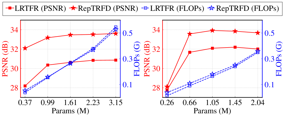
Model Complexity. We vary $\beta_{k}$ to obtain models with different parameter counts and compare them with LRTFR under matched complexity. For LRTFR, the MLP width is adjusted to ensure comparable parameters and FLOPs. Fig. 9 reports PSNR versus model complexity, showing that RepTRFD consistently outperforms LRTFR under similar parameter and FLOP budgets.

Figure 9: PSNR and FLOPs versus parameter count on Airplane ($\text{SR}=0.3$) (left) and Toy ($\text{SD}=0.2$) (right).

Scalability to Higher-Order Tensors. To evaluate the scalability of RepTRFD to higher-order data, we conduct inpainting experiments on color videos. Fig. 10 presents representative results on the Container and Salesman sequences. RepTRFD achieves consistently higher PSNR and SSIM values while producing visually sharper details.

PSNR/SSIM	34.94/0.953	34.48/0.950	35.55/0.954	36.39/0.968
PSNR/SSIM	34.49/0.973	34.09/0.967	35.09/0.974	35.99/0.978
Observed	HLRTF	LRTFR	DRO-TFF	Ours

Figure 10: Visual inpainting results on color videos Container ($\text{SR}=0.1$) and Salesman ($\text{SR}=0.2$).

5 Conclusion

In this work, we presented RepTRFD for multi-dimensional data recovery. Specifically, by analyzing the TR’s frequency behavior, we identified the critical role of high-frequency components and proposed a structured reparameterization of TR factors that significantly facilitates their learning. We further established Lipschitz continuity and derived a variance-preserving initialization for the basis matrices, ensuring stable and effective training. Extensive experiments in various tasks validated our approach. Future work includes extending the framework for Tucker decomposition and block-term tensor decomposition.

Supplementary Material

This supplementary material provides additional technical details and experimental results. In Section A, we present the complete proofs of all theorems in the main paper. Section B describes the model configurations and parameter settings used for the four tasks. Section C reports extended experiments, including ablation studies and practical applications.

Appendix A Detaied Proofs of Theorems

Theorem 1.

Let $\mathcal{X}=\Phi(\mathcal{G}^{(1)},\dots,\mathcal{G}^{(d)})$ be a TR decomposition. Suppose that the mode-2 frequency components of $\mathcal{G}^{(k)}$ beyond a threshold $\Omega_{k}$ are negligible for all $k$, i.e.,

$$\|\big(\mathscr{F}_{2}[\mathcal{G}^{(k)}]\big)_{:\omega_{k}:}\|_{\infty}\leq\epsilon,\ \forall|\omega_{k}|>\Omega_{k},k=1,2,\dots,d,$$

where $\epsilon>0$ is a small constant. Then the reconstructed tensor $\mathcal{X}$ also exhibits attenuated high-frequency content along mode $k$:

$$\|\big(\mathscr{F}_{k}[\mathcal{X}]\big)_{:\omega_{k}:}\|_{\infty}\leq c_{k}\,\epsilon,\ \forall|\omega_{k}|>\Omega_{k},k=1,2,\dots,d,$$

where $c_{k}$ is a constant depending only on the magnitudes of the remaining cores $\{\mathcal{G}^{(j)}\}_{j\neq k}$.

Proof.

In TR decomposition, each element of $\mathcal{X}$ is expressed as

$$\mathcal{X}_{v_{1},\dots,v_{d}}=\operatorname{trace}\!\left(\mathcal{G}^{(1)}_{:v_{1}:}\mathcal{G}^{(2)}_{:v_{2}:}\cdots\mathcal{G}^{(k)}_{:v_{k}:}\cdots\mathcal{G}^{(d)}_{:v_{d}:}\right).$$

By the cyclic property of the trace, we can isolate the $k$-th factor:

$$\mathcal{X}_{v_{1},\dots,v_{d}}=\operatorname{trace}\!\left(\mathbf{M}_{(\neg k)}\cdot\mathcal{G}^{(k)}_{:v_{k}:}\right),$$

where

$$\mathbf{M}_{(\neg k)}=\mathcal{G}^{(k+1)}_{:v_{k+1}:}\cdots\mathcal{G}^{(d)}_{:v_{d}:}\mathcal{G}^{(1)}_{:v_{1}:}\cdots\mathcal{G}^{(k-1)}_{:v_{k-1}:}\in\mathbb{R}^{r_{k+1}\times r_{k}}.$$

For fixed indices $\{v_{j}\}_{j\neq k}$, the matrix $\mathbf{M}_{(\neg k)}$ is constant with respect to $v_{k}$. Expanding the trace gives

$$\mathcal{X}_{v_{1},\dots,v_{d}} =\sum_{p=1}^{r_{k}}\sum_{q=1}^{r_{k+1}}[\mathbf{M}_{(\neg k)}]_{q,p}\,\mathcal{G}^{(k)}_{p,v_{k},q}.$$

Applying the mode-$k$ DFT along the $k$-th dimension, we obtain

$$\big(\mathscr{F}_{k}[\mathcal{X}]\big)_{v_{1},\dots,\omega_{k},\dots,v_{d}}$$

$$=\sum_{v_{k}=1}^{n_{k}}\mathcal{X}_{v_{1},\dots,v_{k},\dots,v_{d}}\cdot[\mathbf{F}_{k}]_{v_{k},\omega_{k}}$$

$$=\sum_{v_{k}=1}^{n_{k}}\left(\sum_{p=1}^{r_{k}}\sum_{q=1}^{r_{k+1}}[\mathbf{M}_{(\neg k)}]_{q,p}\cdot\mathcal{G}^{(k)}_{p,v_{k},q}\right)\cdot[\mathbf{F}_{k}]_{v_{k},\omega_{k}}$$

$$=\sum_{p=1}^{r_{k}}\sum_{q=1}^{r_{k+1}}[\mathbf{M}_{(\neg k)}]_{q,p}\cdot\left(\sum_{v_{k}=1}^{n_{k}}\mathcal{G}^{(k)}_{p,v_{k},q}\cdot[\mathbf{F}_{k}]_{v_{k},\omega_{k}}\right).$$

Using the definition of mode-2 DFT for the TR factor $\mathcal{G}^{(k)}$,

$$\big(\mathscr{F}_{2}[\mathcal{G}^{(k)}]\big)_{p,\omega_{k},q}=\sum_{v_{k}=1}^{n_{k}}\mathcal{G}^{(k)}_{p,v_{k},q}\cdot[\mathbf{F}_{k}]_{v_{k},\omega_{k}},$$

we can rewrite the expression as

$$\big(\mathscr{F}_{k}[\mathcal{X}]\big)_{v_{1},\dots,\omega_{k},\dots,v_{d}}$$

$$=\sum_{p=1}^{r_{k}}\sum_{q=1}^{r_{k+1}}[\mathbf{M}_{(\neg k)}]_{q,p}\cdot\big(\mathscr{F}_{2}[\mathcal{G}^{(k)}]\big)_{p,\omega_{k},q}.$$

We now bound the magnitude of this term. Using the triangle inequality:

$$\left|\big(\mathscr{F}_{k}[\mathcal{X}]\big)_{v_{1},\dots,\omega_{k},\dots,v_{d}}\right|$$

$$\leq\sum_{p=1}^{r_{k}}\sum_{q=1}^{r_{k+1}}\left|[\mathbf{M}_{(\neg k)}]_{q,p}\right|\cdot\left|\big(\mathscr{F}_{2}[\mathcal{G}^{(k)}]\big)_{p,\omega_{k},q}\right|.$$

By the assumption on $\mathcal{G}^{(k)}$, for all $|\omega_{k}|>\Omega_{k}$, we have

$$\left|\big(\mathscr{F}_{2}[\mathcal{G}^{(k)}]\big)_{p,\omega_{k},q}\right|\leq\epsilon.$$

Substituting this bound:

$$\left|\big(\mathscr{F}_{k}[\mathcal{X}]\big)_{v_{1},\dots,\omega_{k},\dots,v_{d}}\right| \leq\epsilon\cdot\left(\sum_{p=1}^{r_{k}}\sum_{q=1}^{r_{k+1}}\left|[\mathbf{M}_{(\neg k)}]_{q,p}\right|\right).$$

Defining the constant $c_{k}$ as the maximum possible sum of magnitudes of the product of the remaining cores:

$$c_{k}:=\max_{\{v_{j}\}_{j\neq k}}\sum_{p=1}^{r_{k}}\sum_{q=1}^{r_{k+1}}\left|[\mathbf{M}_{(\neg k)}]_{q,p}\right|,$$

we obtain the final bound for the infinity norm over the spatial indices $\{v_{j}\}_{j\neq k}$:

$$\|\big(\mathscr{F}_{k}[\mathcal{X}]\big)_{:\omega_{k}:}\|_{\infty}\leq c_{k}\,\epsilon,\qquad\forall|\omega_{k}|>\Omega_{k}.$$

This completes the proof. ∎

Theorem 2.

Consider a TR factor $\mathcal{G}$ reparameterized as $\mathcal{G}=\mathcal{C}\times_{3}\mathbf{B}$, where $\mathcal{C}\in\mathbb{R}^{r_{1}\times n\times R_{2}}$ is a trainable tensor and $\mathbf{B}\in\mathbb{R}^{r_{2}\times R_{2}}$ is a fixed basis. Let $\mathsf{L}(\omega)$ be the loss associated with frequency $\omega$. For any $\omega_{\rm high}>\omega_{\rm low}>0$, given any $\epsilon\geq 0$, and fixed indices $p,q$ with $1\leq p\leq r_{1}$ and $1\leq q\leq n$, there exists a matrix $\mathbf{B}$ such that for all $s=1,\dots,R_{2}$,

Proof.

First, from the reparameterization $\mathcal{G}=\mathcal{C}\times_{3}\mathbf{B}$, we have

$$\mathcal{G}_{pqj}=\sum_{s=1}^{R_{2}}\mathcal{C}_{pqs}\mathbf{B}_{js},$$

Viewing $\mathcal{G}_{pq1},\ldots,\mathcal{G}_{pqr_{2}}$ as latent variables dependent on $\mathcal{C}_{pqs}$, by the chain rule we obtain

$$\frac{\partial\mathsf{L}(\omega)}{\partial\mathcal{C}_{pqs}}=\sum_{t=1}^{r_{2}}\frac{\partial\mathsf{L}(\omega)}{\partial\mathcal{G}_{pqt}}\mathbf{B}_{ts}.$$

Next, given two frequencies $\omega_{\rm high}>\omega_{\rm low}>0$ and fixed fiber indices $p,q$, define

$$\tau=\mathop{\mathrm{argmax}}_{j}\left|\frac{\partial\mathsf{L}(\omega_{\rm high}))}{\partial\mathcal{G}_{pqj}}\Big/\frac{\partial\mathsf{L}(\omega_{\rm low})}{\partial\mathcal{G}_{pqj}}\right|.$$

By the triangle inequality, we have

$$\left|\frac{\partial\mathsf{L}(\omega_{\rm high})}{\partial\mathcal{C}_{pqs}}\Big/\frac{\partial\mathsf{L}(\omega_{\rm low})}{\partial\mathcal{C}_{pqs}}\right|$$

$$=\left|\frac{\frac{\partial\mathsf{L}(\omega_{\rm high})}{\partial\mathcal{G}_{pq\tau}}\mathbf{B}_{\tau s}+\sum_{t\neq\tau}\frac{\partial\mathsf{L}(\omega_{\rm high})}{\partial\mathcal{G}_{pqt}}\mathbf{B}_{ts}}{\frac{\partial\mathsf{L}(\omega_{\rm low})}{\partial\mathcal{G}_{pq\tau}}\mathbf{B}_{\tau s}+\sum_{t\neq\tau}\frac{\partial\mathsf{L}(\omega_{\rm low})}{\partial\mathcal{G}_{pqt}}\mathbf{B}_{ts}}\right|$$

$$\geq\frac{\left|\frac{\partial\mathsf{L}(\omega_{\rm high})}{\partial\mathcal{G}_{pq\tau}}\mathbf{B}_{\tau s}\right|-\left|\sum_{t\neq\tau}\frac{\partial\mathsf{L}(\omega_{\rm high})}{\partial\mathcal{G}_{pqt}}\mathbf{B}_{ts}\right|}{\left|\frac{\partial\mathsf{L}(\omega_{\rm low})}{\partial\mathcal{G}_{pq\tau}}\mathbf{B}_{\tau s}\right|+\left|\sum_{t\neq\tau}\frac{\partial\mathsf{L}(\omega_{\rm low})}{\partial\mathcal{G}_{pqt}}\mathbf{B}_{ts}\right|}.$$

For the elements of $\mathbf{B}$, construct $\mathbf{B}_{ts}$ such that for $s=1,\ldots,R_{2}$, $|\mathbf{B}_{ts}|\leq\alpha$ when $t\neq\tau$ and $\mathbf{B}_{\tau s}=1$, where $\alpha>0$ is a positive upper bound. Define

$$M_{1}=\sum_{t\neq\tau}\left|\frac{\partial\mathsf{L}(\omega_{\rm high})}{\partial\mathcal{G}_{pqt}}\right|,\qquad M_{2}=\sum_{t\neq\tau}\left|\frac{\partial\mathsf{L}(\omega_{\rm low})}{\partial\mathcal{G}_{pqt}}\right|.$$

Without loss of generality, for any $\epsilon\geq 0$, choose

From the upper bound on $\alpha$, it holds that

$$\left|\sum_{t\neq\tau}\frac{\partial\mathsf{L}(\omega_{\rm high})}{\partial\mathcal{G}_{pqt}}\mathbf{B}_{ts}\right|\leq\alpha M_{1}\leq\left|\frac{\partial\mathsf{L}(\omega_{\rm high})}{\partial\mathcal{G}_{pq\tau}}\right|,$$

which implies

$$\left|\frac{\partial\mathsf{L}(\omega_{\rm high})}{\partial\mathcal{G}_{pq\tau}}\right|-\left|\sum_{t\neq\tau}\frac{\partial\mathsf{L}(\omega_{\rm high})}{\partial\mathcal{G}_{pqt}}\mathbf{B}_{ts}\right|\geq 0.$$

Thus, for fixed $p,q$ and for $s=1,\ldots,R_{2}$, we get

$$\left|\frac{\partial\mathsf{L}(\omega_{\rm high})}{\partial\mathcal{C}_{pqs}}\Big/\frac{\partial\mathsf{L}(\omega_{\rm low})}{\partial\mathcal{C}_{pqs}}\right|$$

$$\geq\frac{\left|\frac{\partial\mathsf{L}(\omega_{\rm high})}{\partial\mathcal{G}_{pq\tau}}\right|-\alpha M_{1}}{\left|\frac{\partial\mathsf{L}(\omega_{\rm low})}{\partial\mathcal{G}_{pq\tau}}\right|+\alpha M_{2}}$$

$$\geq\frac{\left|\frac{\partial\mathsf{L}(\omega_{\rm high})}{\partial\mathcal{G}_{pq\tau}}\right|-\epsilon\left|\frac{\partial\mathsf{L}(\omega_{\rm low})}{\partial\mathcal{G}_{pq\tau}}\right|}{\left|\frac{\partial\mathsf{L}(\omega_{\rm low})}{\partial\mathcal{G}_{pq\tau}}\right|}$$

$$=\max_{j=1,\dots,r_{2}}\left|\frac{\partial\mathsf{L}(\omega_{\rm high}))}{\partial\mathcal{G}_{pqj}}\Big/\frac{\partial\mathsf{L}(\omega_{\rm low})}{\partial\mathcal{G}_{pqj}}\right|-\epsilon.$$

The second inequality is obtained by applying the first upper bound of $\alpha$. This completes the proof. ∎

Remark.

We note that the proof of Theorem 2 provides an existence guarantee, demonstrating that a suitable choice of $\mathbf{B}$ can in principle amplify high-frequency gradients. However, the specific construction in the proof is not employed in practice, as the optimal index $\tau$ is dynamic and depends on the data, making it infeasible to pre-specify. Instead, we adopt the principled Xavier-style initialization described in Theorem 3, which preserves variance in both forward and backward passes. This provides a stable starting point for optimization while allowing the model to learn from a fully expressive random state.

Theorem 3.

Suppose the entries of $\mathbf{B}^{(k)}$ in the reparameterized TR factor are sampled independently from a uniform distribution as

$$\mathbf{B}^{(k)}_{ij}\sim\mathcal{U}\left(-\sqrt{\tfrac{6}{r_{k+1}+R_{k+1}}},\ \sqrt{\tfrac{6}{r_{k+1}+R_{k+1}}}\right),\forall i,j,k,$$

then the variances in both the forward and backward passes are preserved.

Proof.

We derive the variance of the initialization parameter $\sigma_{\mathbf{B}}^{2}$ by enforcing variance preservation in both the forward and backward passes.

Forward pass. Each element of $\mathcal{G}^{(k)}$ is computed as

$$\mathcal{G}_{pqj}^{(k)}=\sum_{s=1}^{R_{k+1}}\mathcal{C}^{(k)}_{pqs}\mathbf{B}_{js}^{(k)}.$$

Since both $\mathcal{C}^{(k)}$ and $\mathbf{B}^{(k)}$ are zero-mean and independent, the variance of $\mathcal{G}^{(k)}_{pqj}$ is

$$\operatorname{Var}(\mathcal{G}_{pgj}^{(k)})=R_{k+1}\sigma_{\mathcal{C}}^{2}\sigma_{\mathbf{B}}^{2}.$$

To maintain signal variance, we require that

$$\mathrm{Var}(\mathcal{G}_{pgj}^{(k)})=\mathrm{Var}(\mathcal{C}_{pqj}^{(k)})=\sigma_{\mathcal{C}}^{2},$$

which gives

$$\sigma_{\mathbf{B}}^{2}=\frac{1}{\hat{R}_{i+1}}.$$

Backward pass. During backpropagation, the gradient of the loss function with respect to $\mathcal{C}^{(k)}_{pqj}$ is

$$\frac{\partial\mathsf{L}}{\partial\mathcal{C}_{pqj}^{(k)}}=\sum_{t=1}^{r_{k+1}}\frac{\partial\mathsf{L}}{\partial\mathcal{G}_{pqt}^{(k)}}\frac{\partial\mathcal{G}_{pqt}^{(k)}}{\partial\mathcal{C}_{pqj}^{(k)}}=\sum_{t=1}^{r_{k+1}}\frac{\partial\mathsf{L}}{\partial\mathcal{G}_{pqt}^{(k)}}\mathbf{B}_{ts}^{(k)}.$$

Assuming i.i.d. gradients with $\operatorname{Var}\big(\frac{\partial\mathsf{L}}{\partial\mathcal{G}_{pqt}^{(k)}}\big)=\sigma_{\nabla\mathcal{G}}^{2}$, we obtain

$$\operatorname{Var}\left(\frac{\partial\mathsf{L}}{\partial\mathcal{C}_{pqj}^{(k)}}\right)=R_{i+1}\sigma_{\nabla\mathcal{G}}^{2}\sigma_{\mathbf{B}}^{2}.$$

To preserve the variance of the backpropagated gradients, we require

$$\sigma_{\mathbf{B}}^{2}=\frac{1}{R_{i+1}}.$$

Following the principle of Xavier Glorot initialization [9], which balances the forward and backward variance constraints, we take the harmonic mean of the two bounds, yielding

$$\sigma_{\mathbf{B}}^{2}=\frac{2}{r_{k+1}+R_{k+1}}.$$

Since a zero-mean uniform distribution $\mathcal{U}(-a,a)$ has variance $\operatorname{Var}=a^{2}/3$, setting $a=\sqrt{6/(r_{k+1}+R_{k+1})}$ makes its variance exactly equal to $\sigma_{\mathbf{B}}^{2}$, yielding the final form

$$\mathbf{B}^{(k)}_{ij}\sim\mathcal{U}\left(-\sqrt{\tfrac{6}{r_{k+1}+R_{k+1}}},\ \sqrt{\tfrac{6}{r_{k+1}+R_{k+1}}}\right),\qquad\forall i,j,k,$$

which completes the proof. ∎

Remark.

The analysis in Theorem 3 is not restricted to Xavier initialization and naturally extends to other variance-preserving schemes. In particular, enforcing forward-pass variance preservation under Kaiming initialization yields $\mathbf{B}^{(k)}_{ij}\sim\mathcal{U}\left(-\sqrt{\tfrac{6}{R_{k+1}}},\ \sqrt{\tfrac{6}{R_{k+1}}}\right)$. Numerical results are provided in Section C.

Theorem 4.

Let $g_{\phi}(\mathbf{v}):\mathbb{R}^{d}\to\mathbb{R}$ be defined as

$$g_{\phi}(\mathbf{v})=\Phi(g_{\phi_{1}}(v_{1})\times_{3}\mathbf{B}^{(1)},\dots,g_{\phi_{d}}(v_{d})\times_{3}\mathbf{B}^{(d)}),$$

where $\mathbf{v}=[v_{1},\dots,v_{d}]^{\mathrm{T}}\in\mathbb{R}^{d}$ denotes the coordinate vector, and each $\mathbf{B}^{(k)}\in\mathbb{R}^{r_{k+1}\times R_{k+1}}$ is a fixed basis. Assume for each mode $k=1,\dots,d$, the following conditions hold:

• $g_{\phi_{k}}(\cdot)$ is an $L_{k}$-layer MLP with activation function $\sigma(\cdot)$ that is $\kappa$-Lipschitz continuous;

• the spectral norm of each weight matrix in $g_{\phi_{k}}(\cdot)$ is bounded by $\eta$;

• the output is bounded: $\sup_{v_{k}}\|g_{\phi_{k}}(v_{k})\|_{F}\leq C_{k}<\infty$.

Then, $g_{\phi}(\mathbf{v})$ is globally Lipschitz continuous, i.e.,

$$|g_{\phi}(\mathbf{v})-g_{\phi}(\mathbf{v}^{\prime})|\leq\delta\|\mathbf{v}-\mathbf{v}^{\prime}\|_{2},$$

where the global Lipschitz constant $\delta=\sqrt{\sum_{k=1}^{d}\delta_{k}^{2}}$, and $\delta_{k}=(\kappa\eta)^{L_{k}}\cdot\|\mathbf{B}_{k}\|_{2}\cdot\left(\prod_{j\neq k}C_{j}\right)$.

Proof.

For the $i$-th layer of the $k$-th MLP, defined as

$$g_{i}^{(k)}(\mathbf{x})=\sigma(\mathbf{W}_{i}\mathbf{x}+\mathbf{b}_{i}),$$

the Lipschitz constant is bounded by the product of the activation’s constant and the affine transformation’s constant:

$$L(g_{i}^{(k)})\leq L(\sigma)\cdot L(\mathbf{W}_{i}\mathbf{x}+\mathbf{b}_{i})\leq\kappa\cdot\|\mathbf{W}_{i}\|_{2}\leq\kappa\eta.$$

Hence, for an $L_{k}$-layer MLP $g_{\phi_{k}}$, the overall Lipschitz constant satisfies

$$L_{g}^{(k)}\leq\prod_{i=1}^{L_{k}}L(g_{i}^{(k)})\leq(\kappa\eta)^{L_{k}}.$$

We then have

$$\left\lVert\mathcal{G}_{:v_{k}:}^{(k)}-\mathcal{G}_{:v^{\prime}_{k}:}^{(k)}\right\rVert_{F}$$

$$=\|g_{\phi_{k}}(v_{k})\times_{3}\mathbf{B}^{(k)}-g_{\phi_{k}}(v^{\prime}_{k})\times_{3}\mathbf{B}^{(k)})\|_{F}$$

$$=\|(g_{\phi_{k}}(v_{k})-g_{\phi_{k}}(v^{\prime}_{k}))\times_{3}\mathbf{B}_{k}\|_{F}$$

$$\leq\|g_{\phi_{k}}(v_{k})-g_{\phi_{k}}(v^{\prime}_{k})\|_{F}\cdot\|\mathbf{B}_{k}\|_{2}$$

$$\leq(\kappa\eta)^{L_{k}}\|\mathbf{B}_{k}\|_{2}\cdot|v_{k}-v^{\prime}_{k}|.$$

Let $\mathbf{G}^{(k)}_{v_{k}}=\mathcal{G}^{(k)}_{:v_{k}:}\in\mathbb{R}^{r_{k}\times r_{k+1}}$, $\mathbf{M}_{(\neg k)}=\mathbf{G}^{(k+1)}_{v_{k+1}}\cdots\mathbf{G}^{(d)}_{v_{d}}\mathbf{G}^{(1)}_{v_{1}}\cdots\mathbf{G}^{(k-1)}_{v_{k-1}}\in\mathbb{R}^{r_{k+1}\times r_{k}}$, and denote by $\mathbf{v}_{k}^{\prime}=(v_{1},\dots,v_{k-1},v_{k}^{\prime},v_{k+1},\dots,v_{d})$ the coordinate vector differing from $\mathbf{v}$ only at the $k$-th entry. Then,

$$|g_{\phi}(\mathbf{v})-g_{\phi}(\mathbf{v}^{\prime}_{k})|$$

$$=\left|\operatorname{trace}\left(\mathbf{M}_{(\neg k)}\cdot\mathbf{G}^{(k)}_{v_{k}}\right)-\operatorname{trace}\left(\mathbf{M}_{(\neg k)}\cdot\mathbf{G}^{(k)}_{v^{\prime}_{k}}\right)\right|$$

$$\leq\|\mathbf{M}\|_{F}\cdot\left\lVert\mathbf{G}^{(k)}_{v_{k}}-\mathbf{G}^{(k)}_{v^{\prime}_{k}}\right\rVert_{F}$$

$$\leq\prod_{j\neq k}\left\lVert\mathbf{G}_{v_{j}}^{(j)}\right\rVert_{F}\cdot\left\lVert\mathcal{G}_{:v_{k}:}^{(k)}-\mathcal{G}_{:v^{\prime}_{k}:}^{(k)}\right\rVert_{F}$$

$$\leq(\kappa\eta)^{L_{k}}\cdot\|\mathbf{B}_{k}\|_{2}\cdot\prod_{j\neq k}C_{j}\cdot|v_{k}-v^{\prime}_{k}|.$$

Aggregating across all dimensions yields

$$|g_{\phi}(\mathbf{v})-g_{\phi}(\mathbf{v}^{\prime})|$$

$$\leq\sum_{k=1}^{d}|g_{\phi}(\mathbf{v})-g_{\phi}(\mathbf{v}^{\prime}_{k})|$$

$$\leq\sum_{k=1}^{d}(\kappa\eta)^{L_{k}}\cdot\|\mathbf{B}_{k}\|_{2}\cdot\prod_{j\neq k}C_{j}\cdot|v_{k}-v^{\prime}_{k}|.$$

Finally, applying the Cauchy–Schwarz inequality gives

$$|g_{\phi}(\mathbf{v})-g_{\phi}(\mathbf{v}^{\prime})|$$

$$\leq\sqrt{\sum_{k=1}^{d}\left((\kappa\eta)^{L_{k}}\cdot\|\mathbf{B}_{k}\|_{2}\cdot\prod_{j\neq k}C_{j}\right)^{2}}\cdot\left\lVert\mathbf{v}-\mathbf{v}^{\prime}\right\rVert_{2},$$

which completes the proof. ∎

Appendix B Task-Specific Losses and Settings

In this section, we provide the loss formulations and hyperparameter settings for the four tasks studied in our experiments. Recall that

$$g_{\phi}(\{\mathbf{v}_{k}\}_{k=1}^{d})=\Phi(g_{\phi_{1}}(\mathbf{v}_{1})\times_{3}\mathbf{B}^{(1)},\dots,g_{\phi_{d}}(\mathbf{v}_{d})\times_{3}\mathbf{B}^{(d)})$$

denotes the RepTRFD reconstruction with learnable parameters $\phi$ and fixed bases $\{\mathbf{B}^{(k)}\}_{k=1}^{d}$. The main hyperparameters in our model include the TR rank $[r_{1},\dots,r_{d}]$, the latent tensor expansion factor $\beta$, the frequency parameter $\omega_{0}$ for the sinusoidal mapping, and the number of layers in each branch network. Each task is formulated as a single optimization problem minimizing a combination of a data fidelity term and an optional regularization term.

Image and Video Inpainting, which aims to reconstruct missing regions from partially observed visual data:

$$\min_{\phi}\|\mathscr{P}_{\Omega}(g_{\phi}(\{\mathbf{v}_{k}\}_{k=1}^{d})-\mathcal{O})\|_{F}^{2}+\gamma_{1}\|g_{\phi}(\{\mathbf{v}_{k}\}_{k=1}^{d})\|_{\rm TV}$$

$$+\gamma_{2}\|g_{\phi}(\{\mathbf{v}_{k}\}_{k=1}^{d})\|_{\rm SSTV},$$

where $\mathcal{O}$ is the observed incomplete data, and $\mathscr{P}_{\Omega}(\cdot)$ denotes projection onto observed entries. The total variation (TV) is defined along spatial dimensions as $\|\mathcal{X}\|_{\rm TV}=\|\nabla_{v_{1}}\mathcal{X}\|_{1}+\|\nabla_{v_{2}}\mathcal{X}\|_{1}$, and the spatial-spectral TV (SSTV) involves the spectral dimension, defined as $\|\mathcal{X}\|_{\rm SSTV}=\|\nabla_{v_{1}}\nabla_{v_{3}}\mathcal{X}\|_{1}+\|\nabla_{v_{2}}\nabla_{v_{3}}\mathcal{X}\|_{1}$. For all modes $k$, $r_{k}=20$ and $\beta=10$. Frequency parameter $\omega_{0}$ is set to 90 for color images and videos, and 120 for MSIs and HSIs. Branch layers $[L_{1},L_{2},L_{3}]$ are set to $[1,1,2]$ for color images and videos, and $[1,1,1]$ for MSIs and HSIs. Regularization parameters are set as follows: $\gamma_{1}=\gamma_{2}=5\times 10^{-5}$ for color images; $\gamma_{1}=5\times 10^{-5}$ and $\gamma_{2}=5\times 10^{-4}$ for MSIs and videos; $\gamma_{1}=5\times 10^{-6}$ and $\gamma_{2}=5\times 10^{-5}$ for HSIs.

Image Denoising, which aims to recover clean images from noisy observations:

$$\min_{\phi}\|g_{\phi}(\{\mathbf{v}_{k}\}_{k=1}^{d})-\mathcal{O}\|_{F}^{2}+\gamma_{1}\|g_{\phi}(\{\mathbf{v}_{k}\}_{k=1}^{d})\|_{\rm TV}$$

$$+\gamma_{2}\|g_{\phi}(\{\mathbf{v}_{k}\}_{k=1}^{d})\|_{\rm SSTV},$$

where $\mathcal{O}$ is the observed noisy data. For all modes $k$, $r_{k}=16$ and $\beta=5$. Frequency parameter $\omega_{0}$ is set to 120, and branch layers $[L_{1},L_{2},L_{3}]$ are $[1,1,2]$. Regularization weights are set as $\gamma_{1}=\gamma_{2}=10^{-4}$ for MSIs and $\gamma_{1}=\gamma_{2}=10^{-5}$ for HSIs.

Image Super-Resolution, which seeks to reconstruct high-resolution images from their low-resolution counterparts:

$$\min_{\phi}\|\operatorname{Down}(g_{\phi}(\{\mathbf{v}_{k}\}_{k=1}^{d}))-\mathcal{O}\|_{F}^{2}+\gamma_{1}\|g_{\phi}(\{\mathbf{v}_{k}\}_{k=1}^{d})\|_{\rm TV},$$

where $\operatorname{Down}(\cdot)$ is the downsampling operator and $\mathcal{O}$ is the low-resolution observation. For all modes $k$, $r_{k}=20$ and $\beta=10$. Frequency parameter $\omega_{0}$ is set to 90, branch layers $[L_{1},L_{2},L_{3}]$ are $[1,1,2]$, and $\gamma_{1}=5\times 10^{-5}$.

Point Cloud Recovery, which aims to infer continuous point-wise attributes from partially observed point cloud data:

$$\min_{\phi}\sum_{k=1}^{N}(g_{\phi}(\mathbf{v}_{k})-\mathbf{O}_{k,5})^{2},$$

where the observed data $\mathbf{O}\in\mathbb{R}^{N\times 5}$ contains $N$ points, with each row encoding spatial coordinates $(x,y,z)$, color information $c$, and a scalar value $s$. Here, $\mathbf{v}_{k}=(x_{k},y_{k},z_{k},c_{k})$ is the input coordinate-color vector of the $k$-th point, and $\mathbf{O}_{k,5}$ is the corresponding observed scalar value. For all modes $k$, $r_{k}=20$ and $\beta=3$. Frequency parameter $\omega_{0}$ is set to 240, and all branches use a single layer.

Appendix C Supplementary Experimental Results

C.1 Additional Ablation Studies

Effectiveness of the Fixed Basis Strategy. To validate the necessity of a fixed basis, we compare our proposed strategy with a variant where the basis matrices are treated as learnable parameters. As illustrated in Fig. S1, although both methods exhibit similar convergence speeds in the early stage, they diverge significantly in later iterations. The learnable basis model reaches a lower peak PSNR and subsequently suffers from performance degradation. This phenomenon suggests that allowing basis matrices to vary introduces excessive degrees of freedom, causing the model to overfit high-frequency noise or drift away from the variance-preserving initialization. In contrast, our fixed basis strategy acts as a structural regularizer, maintaining improved stability and consistently higher reconstruction quality throughout the training process.

Figure S1: Impact of the fixed basis strategy on denoising performance for the MSIs Toy (left) and Face (right) with $\text{SD}=0.2$.

Hyperparameter Sensitivity Analysis. We investigate the sensitivity of two key hyperparameters in our framework, the TR rank and the frequency scaling parameter $\omega_{0}$. Experiments are conducted on the MSI datasets Toy and Face for denoising with $\text{SD}=0.2$. Fig. S2 presents the variation of PSNR with different values of these hyperparameters. The results indicate that our method is relatively robust to the choice of both the TR rank and $\omega_{0}$, maintaining high reconstruction quality across a wide range of settings. In addition, we examine the interaction between the regularization parameter $\beta$ and the frequency scaling parameter $\omega_{0}$. As shown in Fig. S3, RepTRFD maintains stable performance over a broad range of parameter combinations.

Figure S2: PSNR variation with TR rank and frequency scaling $\omega_{0}$ for MSI denoising on Toy (left) and Face (right) datasets with $\text{SD}=0.2$.

Figure S3: PSNR sensitivity to hyperparameters $\beta$ and $\omega_{0}$ for inpainting on Airplane ($\text{SR}=0.3$) (left) and denoising on Toy ($\text{SD}=0.2$) (right).

Impact of Explicit Regularization. To disentangle the effect of our reparameterized architecture from that of explicit smoothness priors, we further evaluate a variant of RepTRFD trained solely with a data fidelity loss, i.e., without incorporating TV or SSTV regularization. We conduct experiments on both inpainting and super-resolution tasks, contrasting performance against the representative functional tensor baseline, LRTFR [21]. As reported in Tables S1 and S2, even without explicit regularization, our method yields significant PSNR gains over LRTFR across all datasets. This demonstrates the inherent advantage of the proposed reparameterization scheme in capturing latent structures. When regularization is incorporated, performance is further boosted, confirming its complementary role in enhancing spatial smoothness and mitigating artifacts. These results collectively verify that the primary performance improvement stems from the RepTRFD architecture itself, while explicit regularization serves as an effective refinement mechanism.

Table S1: PSNR comparison on image and video inpainting at $\text{SR}=0.2$ under different regularization settings.

Data	LRTFR (Baseline)	RepTRFD (w/o TV)	RepTRFD (w/ TV)
Airplane	27.21	29.37	30.45
Flowers	44.27	48.53	50.13
Botswana	41.86	44.94	45.27
Carphone	30.18	31.86	32.58

Table S2: PSNR comparison on $\times 4$ image super-resolution under different regularization settings.

Data	LRTFR (Baseline)	RepTRFD (w/o TV)	RepTRFD (w/ TV)
Lion	28.10	30.37	31.01
Parrot	27.81	29.79	30.39

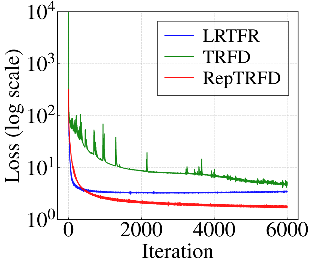
Convergence Behavior. To evaluate the effect of the proposed reparameterization on optimization efficiency, we compare the training loss curves of TRFD, LRTFR, and RepTRFD under matched parameter budgets. Fig. S4 shows the training loss curves of TRFD, LRTFR, and RepTRFD under matched parameter settings. RepTRFD converges faster and reaches a lower loss, demonstrating improved convergence behavior.

Figure S4: Loss curve on the color image Airplane ($\text{SR}=0.3$).

Initialization Scheme. To examine whether the theoretical analysis depends on a specific variance-preserving strategy, we further compare Xavier and Kaiming initialization schemes. Under Kaiming initialization with forward-pass variance preservation, the basis entries follow $\mathbf{B}^{(k)}_{ij}\sim\mathcal{U}\!\left(-\sqrt{\tfrac{6}{R_{k+1}}},\ \sqrt{\tfrac{6}{R_{k+1}}}\right)$. Table S3 reports the reconstruction performance on four datasets with $\text{SR}=0.2$. We observe that the two initialization strategies yield highly comparable results across all datasets, with only marginal differences. This indicates that our framework is robust to the specific choice of variance-preserving initialization and that the theoretical analysis naturally extends beyond Xavier initialization.

Table S3: PSNR results of different variance-preserving initialization schemes on multiple datasets with $\text{SR}=0.2$.

Scheme	Airplane	Toy	Botswana	News
Kaiming	30.23	48.59	45.30	34.75
Xavier	30.45	48.67	45.27	34.90

C.2 Extended Experimental Results

Extended Inpainting Results. To provide a more comprehensive evaluation, we further include extensive qualitative and quantitative comparisons under various SRs and across diverse data modalities. As shown in Fig. S5, we visualize representative inpainting results on RGB, MSI, HSI, and video datasets, covering a wide range of missing patterns and SRs. The visual comparisons consistently demonstrate that our method yields clearer structural details and fewer artifacts compared to existing approaches. For quantitative evaluation, we report full numerical results of color image inpainting in Table S4, and summarize results on MSI, HSI, and video sequences in Table S5. These results further confirm the robustness and superiority of our method.

PSNR/SSIM	22.25/0.617	20.85/0.619	25.40/0.781	26.26/0.796	26.89/0.828	26.99/0.856	28.60/0.900	Inf/1.000
PSNR/SSIM	20.99/0.493	20.90/0.501	24.03/0.695	24.97/0.720	28.52/0.871	28.73/0.909	29.82/0.919	Inf/1.000
PSNR/SSIM	21.53/0.547	21.07/0.545	24.86/0.728	25.00/0.744	27.01/0.839	27.29/0.865	28.62/0.907	Inf/1.000
PSNR/SSIM	29.32/0.791	32.24/0.882	33.85/0.929	34.92/0.948	37.19/0.982	36.31/0.962	38.39/0.985	Inf/1.000
PSNR/SSIM	33.13/0.836	36.07/0.904	41.58/0.979	41.47/0.978	43.94/0.991	42.90/0.985	45.29/0.992	Inf/1.000
PSNR/SSIM	30.07/0.781	32.74/0.897	36.43/0.963	35.81/0.949	37.96/0.968	36.60/0.967	39.52/0.977	Inf/1.000
PSNR/SSIM	31.36/0.886	32.38/0.911	35.24/0.962	34.40/0.943	35.78/0.963	35.45/0.962	37.05/0.973	Inf/1.000
PSNR/SSIM	28.71/0.844	29.38/0.861	30.74/0.885	30.18/0.890	31.12/0.918	30.62/0.903	32.58/0.943	Inf/1.000
Observed	TRLRF	FCTN	HLRTF	LRTFR	DRO-TFF	NeurTV	Ours	Ground truth

Figure S5: Visual inpainting results on various datasets. From top to bottom: color images (House, Peppers, Sailboat) with $\text{SR}=0.2$; MSIs (Toy, Flowers) with $\text{SR}=0.05$ and $0.1$, respectively; HSI (Botswana) with $\text{SR}=0.05$; and video sequences (Grandma, Carphone) with $\text{SR}=0.1$ and $0.2$, respectively.

Table S4: Quantitative comparison on color images. PSNR, SSIM, and NRMSE are reported under different SRs.

Data	Method	$\text{SR}=0.05$			$\text{SR}=0.1$			$\text{SR}=0.15$			$\text{SR}=0.2$			$\text{SR}=0.25$			$\text{SR}=0.3$
		PSNR	SSIM	NRMSE	PSNR	SSIM	NRMSE	PSNR	SSIM	NRMSE	PSNR	SSIM	NRMSE	PSNR	SSIM	NRMSE	PSNR	SSIM	NRMSE
Airplane	TRLRF	15.08	0.172	0.218	17.98	0.347	0.156	19.90	0.444	0.125	21.50	0.529	0.104	23.35	0.623	0.084	25.58	0.712	0.065
	FCTN	14.64	0.219	0.229	17.79	0.370	0.159	20.05	0.504	0.123	22.08	0.600	0.097	24.11	0.689	0.077	25.70	0.747	0.064
	HLRTF	18.46	0.396	0.148	21.89	0.598	0.099	24.82	0.746	0.071	26.77	0.811	0.057	27.61	0.795	0.051	29.40	0.852	0.042
	LRTFR	19.66	0.499	0.129	22.09	0.655	0.097	25.57	0.765	0.065	27.21	0.822	0.054	28.60	0.858	0.046	29.38	0.878	0.042
	DRO-TFF	21.08	0.741	0.109	22.71	0.763	0.090	26.28	0.843	0.060	27.64	0.853	0.051	29.17	0.888	0.043	30.37	0.906	0.037
	NeurTV	22.00	0.729	0.098	24.86	0.827	0.071	26.55	0.871	0.058	28.21	0.905	0.048	29.80	0.927	0.040	31.02	0.932	0.035
	Ours	23.44	0.784	0.083	26.33	0.865	0.060	28.53	0.907	0.046	30.45	0.932	0.037	32.05	0.946	0.031	33.61	0.958	0.026
House	TRLRF	15.69	0.208	0.240	17.92	0.360	0.186	20.58	0.520	0.137	22.25	0.617	0.113	23.75	0.694	0.095	25.12	0.751	0.081
	FCTN	15.47	0.248	0.246	18.13	0.424	0.181	19.76	0.545	0.150	20.85	0.619	0.133	22.20	0.681	0.113	24.44	0.756	0.088
	HLRTF	17.93	0.378	0.186	21.48	0.589	0.123	23.93	0.723	0.093	25.40	0.781	0.078	26.76	0.828	0.067	28.19	0.871	0.057
	LRTFR	19.51	0.460	0.155	21.72	0.604	0.120	24.77	0.743	0.084	26.26	0.796	0.071	26.91	0.834	0.066	28.58	0.879	0.054
	DRO-TFF	19.17	0.582	0.161	23.06	0.696	0.103	25.04	0.759	0.082	26.89	0.828	0.066	27.97	0.848	0.058	28.99	0.875	0.052
	NeurTV	21.06	0.651	0.129	23.28	0.761	0.100	25.56	0.820	0.077	26.99	0.856	0.065	28.26	0.881	0.056	29.02	0.910	0.052
	Ours	22.68	0.715	0.107	25.36	0.821	0.079	27.22	0.870	0.064	28.60	0.900	0.054	29.99	0.923	0.046	30.98	0.934	0.041
Pepper	TRLRF	12.97	0.139	0.409	16.83	0.273	0.262	18.77	0.384	0.210	20.99	0.493	0.162	22.92	0.580	0.130	24.23	0.646	0.112
	FCTN	13.86	0.166	0.369	16.24	0.282	0.281	18.82	0.403	0.209	20.90	0.501	0.164	23.02	0.594	0.129	24.37	0.650	0.110
	HLRTF	15.66	0.249	0.300	19.19	0.451	0.200	21.68	0.579	0.150	24.03	0.695	0.114	25.62	0.765	0.095	26.84	0.801	0.083
	LRTFR	15.06	0.289	0.321	20.76	0.537	0.167	22.95	0.655	0.130	24.97	0.720	0.103	26.15	0.767	0.090	27.98	0.796	0.073
	DRO-TFF	18.84	0.502	0.208	23.73	0.730	0.118	26.55	0.824	0.086	28.52	0.871	0.068	30.22	0.906	0.056	31.38	0.923	0.049
	NeurTV	22.14	0.729	0.142	24.69	0.822	0.106	26.99	0.876	0.081	28.73	0.909	0.067	30.37	0.929	0.055	31.46	0.938	0.049
	Ours	23.14	0.755	0.127	26.10	0.854	0.090	28.02	0.878	0.072	29.82	0.919	0.059	31.29	0.935	0.050	32.46	0.945	0.043
Sailboat	TRLRF	15.17	0.197	0.306	17.35	0.324	0.238	19.44	0.438	0.187	21.53	0.547	0.147	22.66	0.606	0.129	24.45	0.683	0.105
	FCTN	14.69	0.209	0.323	17.37	0.362	0.238	18.61	0.434	0.206	21.07	0.545	0.155	22.79	0.631	0.127	24.16	0.687	0.109
	HLRTF	18.12	0.366	0.218	20.98	0.539	0.157	23.07	0.648	0.123	24.86	0.728	0.100	26.35	0.794	0.084	27.66	0.838	0.073
	LRTFR	18.88	0.412	0.200	20.96	0.552	0.157	23.95	0.693	0.111	25.00	0.744	0.099	27.04	0.806	0.078	29.03	0.871	0.062
	DRO-TFF	21.07	0.658	0.155	23.37	0.747	0.119	25.47	0.800	0.093	27.01	0.839	0.078	28.15	0.862	0.069	29.40	0.890	0.059
	NeurTV	21.55	0.663	0.147	23.79	0.778	0.113	25.53	0.819	0.093	27.29	0.865	0.076	28.47	0.888	0.066	29.60	0.916	0.058
	Ours	22.43	0.722	0.133	25.00	0.823	0.099	27.11	0.876	0.077	28.62	0.907	0.065	29.80	0.923	0.057	31.00	0.938	0.049

Table S5: Quantitative comparison on MSIs, HSIs and videos. PSNR, SSIM, and NRMSE are reported under different SRs.

Data	Method	$\text{SR}=0.03$			$\text{SR}=0.05$			$\text{SR}=0.1$			$\text{SR}=0.15$			$\text{SR}=0.2$
		PSNR	SSIM	NRMSE	PSNR	SSIM	NRMSE	PSNR	SSIM	NRMSE	PSNR	SSIM	NRMSE	PSNR	SSIM	NRMSE
Toys $(256\times 256\times 31)$	TRLRF	25.13	0.625	0.189	29.32	0.791	0.117	33.67	0.901	0.071	36.56	0.943	0.051	38.67	0.964	0.040
	FCTN	28.22	0.788	0.132	32.24	0.882	0.083	37.46	0.955	0.046	40.04	0.972	0.034	42.04	0.982	0.027
	HLRTF	30.73	0.880	0.099	33.85	0.929	0.069	40.15	0.982	0.033	42.64	0.988	0.025	45.56	0.993	0.018
	LRTFR	32.95	0.924	0.077	34.92	0.948	0.061	39.95	0.982	0.034	41.87	0.987	0.027	43.64	0.988	0.022
	DRO-TFF	33.88	0.966	0.069	37.19	0.982	0.047	40.62	0.992	0.032	43.73	0.994	0.022	45.75	0.995	0.017
	NeurTV	33.34	0.927	0.073	36.31	0.962	0.052	40.43	0.984	0.032	42.31	0.987	0.026	43.09	0.987	0.024
	Ours	35.16	0.972	0.059	38.39	0.984	0.041	44.04	0.993	0.021	47.16	0.995	0.015	48.67	0.996	0.011
Flowers $(256\times 256\times 31)$	TRLRF	25.38	0.604	0.318	28.57	0.705	0.220	33.13	0.836	0.130	35.79	0.902	0.096	38.81	0.944	0.068
	FCTN	28.31	0.718	0.227	31.17	0.793	0.163	36.07	0.904	0.093	38.61	0.939	0.069	42.22	0.970	0.046
	HLRTF	30.42	0.830	0.178	35.92	0.945	0.095	41.58	0.979	0.049	44.32	0.988	0.036	46.84	0.992	0.027
	LRTFR	32.64	0.884	0.138	37.84	0.956	0.076	41.47	0.978	0.050	43.10	0.982	0.041	44.27	0.986	0.036
	DRO-TFF	37.09	0.970	0.082	39.71	0.982	0.061	43.94	0.991	0.038	46.28	0.994	0.029	47.51	0.995	0.025
	NeurTV	35.61	0.934	0.098	38.67	0.966	0.069	42.90	0.985	0.042	45.12	0.990	0.033	46.54	0.992	0.028
	Ours	37.11	0.970	0.082	40.30	0.983	0.057	45.29	0.992	0.032	48.32	0.995	0.023	50.13	0.996	0.018
Washinton DC $(256\times 256\times 191)$	TRLRF	26.83	0.635	0.258	29.22	0.771	0.196	32.40	0.914	0.136	35.31	0.954	0.097	37.98	0.973	0.071
	FCTN	28.76	0.830	0.207	32.09	0.912	0.141	34.52	0.946	0.106	36.38	0.963	0.086	41.62	0.987	0.047
	HLRTF	35.31	0.957	0.097	38.29	0.976	0.069	41.68	0.988	0.047	45.04	0.994	0.032	46.66	0.995	0.026
	LRTFR	34.08	0.943	0.112	37.42	0.975	0.076	40.72	0.988	0.052	45.08	0.993	0.032	46.56	0.994	0.027
	DRO-TFF	36.83	0.961	0.082	39.22	0.975	0.062	41.62	0.988	0.047	42.84	0.990	0.041	44.13	0.993	0.035
	NeurTV	35.03	0.950	0.100	38.98	0.977	0.063	44.66	0.992	0.033	46.40	0.993	0.027	47.20	0.995	0.025
	Ours	38.44	0.979	0.068	41.97	0.990	0.045	45.62	0.994	0.030	47.26	0.995	0.025	47.96	0.996	0.023
Botswana $(256\times 256\times 145)$	TRLRF	26.89	0.620	0.186	30.07	0.781	0.129	32.08	0.883	0.102	34.12	0.922	0.081	35.49	0.941	0.069
	FCTN	29.32	0.804	0.141	32.74	0.897	0.095	35.36	0.939	0.070	36.22	0.949	0.063	37.70	0.962	0.054
	HLRTF	33.04	0.918	0.092	36.43	0.963	0.062	38.60	0.979	0.048	39.13	0.981	0.045	40.39	0.989	0.039
	LRTFR	32.87	0.906	0.093	35.81	0.949	0.067	37.49	0.964	0.055	40.05	0.980	0.041	41.86	0.986	0.033
	DRO-TFF	34.74	0.945	0.075	37.96	0.968	0.052	40.84	0.981	0.037	41.38	0.982	0.035	42.01	0.984	0.033
	NeurTV	34.23	0.930	0.080	36.60	0.967	0.061	39.32	0.982	0.044	40.25	0.984	0.040	40.74	0.990	0.038
	Ours	37.11	0.965	0.057	39.52	0.977	0.043	42.81	0.987	0.030	44.40	0.990	0.025	45.27	0.992	0.022
News $(144\times 176\times 100)$	TRLRF	23.66	0.687	0.180	25.05	0.751	0.153	26.76	0.812	0.126	28.18	0.857	0.107	30.00	0.895	0.087
	FCTN	24.28	0.710	0.168	25.81	0.776	0.141	27.74	0.837	0.113	29.24	0.877	0.095	31.00	0.915	0.077
	HLRTF	25.28	0.811	0.149	26.61	0.842	0.128	29.64	0.914	0.090	31.28	0.937	0.075	32.37	0.949	0.066
	LRTFR	26.15	0.815	0.135	26.63	0.811	0.128	29.62	0.893	0.091	30.58	0.910	0.081	31.86	0.931	0.070
	DRO-TFF	27.91	0.894	0.110	28.89	0.909	0.099	30.66	0.937	0.080	32.28	0.953	0.067	33.02	0.960	0.061
	NeurTV	26.31	0.811	0.133	27.67	0.842	0.113	30.05	0.902	0.086	31.42	0.919	0.074	32.58	0.939	0.064
	Ours	28.74	0.917	0.100	30.35	0.938	0.083	32.55	0.957	0.065	33.90	0.967	0.055	34.90	0.972	0.049
Carphone $(144\times 176\times 100)$	TRLRF	22.51	0.607	0.156	24.13	0.680	0.129	26.39	0.769	0.100	27.73	0.816	0.085	28.71	0.844	0.076
	FCTN	23.89	0.663	0.133	25.45	0.729	0.111	27.09	0.792	0.092	28.22	0.831	0.081	29.38	0.861	0.071
	HLRTF	24.28	0.661	0.127	25.71	0.732	0.108	28.12	0.817	0.082	29.63	0.859	0.069	30.74	0.885	0.060
	LRTFR	24.23	0.702	0.128	26.33	0.786	0.100	27.77	0.837	0.085	29.32	0.867	0.071	30.18	0.890	0.064
	DRO-TFF	27.80	0.856	0.085	28.69	0.875	0.076	29.61	0.892	0.069	30.67	0.911	0.061	31.12	0.918	0.058
	NeurTV	25.36	0.709	0.112	27.29	0.793	0.090	28.82	0.847	0.075	29.69	0.894	0.068	30.62	0.903	0.061
	Ours	28.24	0.879	0.080	29.19	0.896	0.072	30.74	0.921	0.060	31.81	0.934	0.053	32.58	0.943	0.049

Extended Denoising Results. We further conduct denoising experiments on MSI and HSI data under different noise levels, where Gaussian noise with SD ranging from 0.1 to 0.3 is added independently to all pixels and spectral bands. Fig. S6 provides visual comparisons across MSI (Toys, Balloons) and HSI scenes (KSC, Indian Pines), showing that our method restores cleaner structural details and yields fewer spectral distortions. Corresponding quantitative results are summarized in Table S6, where PSNR, SSIM, and NRMSE are reported across different SD settings.

PSNR/SSIM	30.29/0.734	30.91/0.807	31.89/0.821	32.36/0.870	33.11/0.902	33.19/0.904	33.93/0.921	Inf/1.000
PSNR/SSIM	31.54/0.712	34.73/0.888	35.18/0.918	36.03/0.910	37.21/0.945	37.30/0.947	37.83/0.955	Inf/1.000
PSNR/SSIM	32.58/0.887	33.32/0.902	33.25/0.907	33.52/0.889	34.79/0.930	34.45/0.909	35.56/0.932	Inf/1.000
PSNR/SSIM	33.77/0.894	33.31/0.858	34.24/0.890	33.91/0.873	34.44/0.911	35.16/0.909	35.67/0.914	Inf/1.000
Observed	LRTDTV	DeepTensor	HLRTF	LRTFR	DRO-TFF	NeurTV	Ours	Ground truth

Figure S6: Visual denoising results on MSI Toy and Balloons, and HSI KSC and Indian Pines with $\text{SD}=0.2$.

Table S6: Quantitative comparison for denoising under different noise levels. PSNR, SSIM, and NRMSE are reported.

Data	Method	$\text{SD}=0.1$			$\text{SD}=0.15$			$\text{SD}=0.2$			$\text{SD}=0.25$			$\text{SD}=0.3$
		PSNR	SSIM	NRMSE	PSNR	SSIM	NRMSE	PSNR	SSIM	NRMSE	PSNR	SSIM	NRMSE	PSNR	SSIM	NRMSE
Toys $(256\times 256\times 31)$	LRTDTV	34.85	0.906	0.062	32.17	0.824	0.084	30.29	0.734	0.104	28.79	0.653	0.124	27.65	0.581	0.141
	DeepTensor	35.11	0.902	0.060	32.50	0.875	0.081	30.91	0.807	0.097	29.50	0.760	0.114	28.62	0.672	0.126
	HLRTF	35.70	0.912	0.056	33.30	0.883	0.074	31.89	0.821	0.087	30.78	0.768	0.098	29.46	0.698	0.115
	LRTFR	36.01	0.936	0.054	34.01	0.918	0.068	32.36	0.870	0.082	31.36	0.869	0.092	30.60	0.829	0.101
	DRO-TFF	37.34	0.954	0.046	35.07	0.933	0.060	33.11	0.902	0.075	32.24	0.887	0.083	31.10	0.875	0.095
	NeurTV	36.71	0.951	0.050	35.23	0.920	0.059	33.19	0.904	0.075	32.17	0.876	0.084	31.51	0.863	0.091
	Ours	37.25	0.958	0.047	35.30	0.941	0.059	33.93	0.921	0.069	32.89	0.902	0.077	32.04	0.889	0.085
Face $(256\times 256\times 31)$	LRTDTV	36.85	0.883	0.090	34.11	0.788	0.123	32.26	0.701	0.152	30.55	0.615	0.185	29.24	0.528	0.216
	DeepTensor	37.36	0.926	0.014	35.51	0.904	0.017	34.06	0.859	0.020	32.62	0.814	0.023	31.87	0.732	0.026
	HLRTF	38.49	0.922	0.074	36.40	0.882	0.095	34.67	0.835	0.115	33.37	0.792	0.134	32.30	0.754	0.152
	LRTFR	39.09	0.935	0.069	36.81	0.896	0.090	35.13	0.858	0.109	33.91	0.821	0.126	33.01	0.808	0.140
	DRO-TFF	40.00	0.964	0.062	37.94	0.937	0.079	36.37	0.920	0.095	35.20	0.900	0.109	34.71	0.887	0.115
	NeurTV	40.51	0.968	0.059	38.46	0.949	0.075	36.78	0.927	0.091	35.77	0.914	0.102	35.22	0.902	0.108
	Ours	40.80	0.970	0.057	39.16	0.957	0.069	37.89	0.945	0.080	36.92	0.933	0.089	36.12	0.921	0.098
Washington DC $(256\times 256\times 191)$	LRTDTV	34.32	0.924	0.109	32.83	0.896	0.129	31.71	0.869	0.147	30.84	0.845	0.163	30.12	0.823	0.177
	DeepTensor	36.01	0.955	0.090	33.80	0.917	0.116	32.32	0.891	0.137	30.92	0.849	0.161	30.16	0.816	0.176
	HLRTF	36.27	0.959	0.087	34.17	0.927	0.111	32.75	0.913	0.131	31.60	0.892	0.149	30.85	0.879	0.162
	LRTFR	35.78	0.953	0.092	34.22	0.934	0.110	33.02	0.914	0.127	32.09	0.895	0.141	31.34	0.880	0.154
	DRO-TFF	36.65	0.948	0.083	35.26	0.934	0.098	34.26	0.919	0.110	33.35	0.904	0.122	32.57	0.885	0.133
	NeurTV	37.06	0.960	0.079	35.29	0.929	0.097	33.86	0.910	0.115	32.79	0.891	0.130	31.92	0.869	0.144
	Ours	37.96	0.971	0.072	36.32	0.957	0.087	35.08	0.945	0.100	34.16	0.932	0.111	33.37	0.918	0.122
Salinas $(217\times 217\times 224)$	LRTDTV	40.13	0.957	0.053	38.19	0.938	0.066	36.82	0.920	0.077	35.83	0.907	0.087	35.01	0.891	0.095
	DeepTensor	40.25	0.952	0.052	38.69	0.938	0.062	37.05	0.921	0.075	36.07	0.902	0.084	35.47	0.896	0.090
	HLRTF	40.20	0.958	0.052	38.85	0.943	0.061	37.50	0.928	0.071	36.52	0.918	0.080	36.06	0.907	0.084
	LRTFR	40.50	0.963	0.051	39.16	0.953	0.059	37.98	0.943	0.068	36.98	0.932	0.076	36.18	0.921	0.083
	DRO-TFF	40.39	0.960	0.051	39.36	0.955	0.058	38.44	0.949	0.064	37.79	0.936	0.069	37.32	0.937	0.073
	NeurTV	41.66	0.966	0.044	40.25	0.961	0.052	39.64	0.954	0.056	38.61	0.939	0.063	37.65	0.930	0.070
	Ours	42.77	0.973	0.040	41.23	0.965	0.046	40.19	0.955	0.052	39.37	0.947	0.058	38.60	0.938	0.063

Extended Super-Resolution Results. To further demonstrate the generalization ability of RepTRFD in recovering fine structural details under high upscaling factors, we provide additional $\times 4$ visual super-resolution results on the DIV2K dataset, as shown in Fig. S7. Compared with both INR (PEMLP [25], SIREN [37], Gauss [30], WIRE [34], and FINER [17]) and tensor functional representation methods (LRTFR [21]), our approach produces sharper edges, cleaner texture patterns, and fewer artifacts. The quantitative results (PSNR/SSIM) shown above each image further verify the visual comparisons, where RepTRFD consistently achieves the best performance across all samples.

21.57/0.585	26.25/0.743	26.15/0.723	27.05/0.808	26.80/0.751	25.15/0.684	27.38/0.852	PSNR/SSIM
26.99/0.724	29.69/0.804	29.21/0.789	30.42/0.830	30.19/0.800	29.14/0.795	30.88/0.864	PSNR/SSIM
22.30/0.588	26.79/0.793	26.14/0.763	27.71/0.828	27.12/0.788	26.64/0.786	28.09/0.868	PSNR/SSIM
24.78/0.575	25.79/0.609	25.40/0.591	26.59/0.643	26.35/0.616	25.54/0.600	26.87/0.673	PSNR/SSIM
23.19/0.633	24.85/0.740	23.88/0.726	25.75/0.790	25.29/0.749	24.54/0.743	26.15/0.843	PSNR/SSIM
PEMLP	SIREN	Gauss	WIRE	FINER	LRTFR	Ours	Ground truth

Figure S7: Visual super-resolution results at $\times 4$ scaling on the DIV2K dataset.

Extended Point Cloud Recovery Results. Fig. S8 presents extended visual results for point cloud recovery under different SRs. We compare the proposed RepTRFD with several INR (PEMLP [25], SIREN [37], Gauss [30], WIRE [34], and FINER [17]) and tensor functional representation methods (LRTFR [21]). Across all tested SRs, our method consistently reconstructs more accurate surface geometry and fine structures, as reflected by the lower NRMSE values shown above each reconstruction. These results demonstrate the superior performance of RepTRFD in point cloud recovery.

NRMSE	NRMSE 0.079	NRMSE 0.077	NRMSE 0.080	NRMSE 0.076	NRMSE 0.076	NRMSE 0.074	NRMSE 0.066	NRMSE 0.000
NRMSE	NRMSE 0.086	NRMSE 0.085	NRMSE 0.086	NRMSE 0.084	NRMSE 0.085	NRMSE 0.088	NRMSE 0.072	NRMSE 0.000
NRMSE	NRMSE 0.094	NRMSE 0.085	NRMSE 0.083	NRMSE 0.080	NRMSE 0.082	NRMSE 0.093	NRMSE 0.079	NRMSE 0.000
NRMSE	NRMSE 0.114	NRMSE 0.104	NRMSE 0.109	NRMSE 0.100	NRMSE 0.102	NRMSE 0.112	NRMSE 0.092	NRMSE 0.000
NRMSE	NRMSE 0.149	NRMSE 0.142	NRMSE 0.149	NRMSE 0.127	NRMSE 0.147	NRMSE 0.149	NRMSE 0.112	NRMSE 0.000
NRMSE	NRMSE 0.112	NRMSE 0.111	NRMSE 0.123	NRMSE 0.106	NRMSE 0.110	NRMSE 0.114	NRMSE 0.093	NRMSE 0.000
Observed	PEMLP	SIREN	Gauss	WIRE	FINER	LRTFR	Ours	Ground truth

Figure S8: Visual comparisons on point cloud recovery over six objects at three SRs: $\text{SR}=0.1$ (Frog, Duck), $\text{SR}=0.15$ (PetterRabbit, Mario), and $\text{SR}=0.2$ (Doll, Cola).

References

- [1] (2016) Hyperspectral image denoising using spatio-spectral total variation. IEEE Geoscience and Remote Sensing Letters 13 (3), pp. 442–446. Cited by: §3.3.
- [2] (2017) Ntire 2017 challenge on single image super-resolution: dataset and study. In Proceedings of the IEEE Conference on Computer Vision and Pattern Recognition Workshops, pp. 126–135. Cited by: §4.2.
- [3] (2024) Batch normalization alleviates the spectral bias in coordinate networks. In Proceedings of the IEEE/CVF Conference on Computer Vision and Pattern Recognition, pp. 25160–25171. Cited by: §2, §2.
- [4] (1970) Analysis of individual differences in multidimensional scaling via an -way generalization of ‘Eckart-Young’ decomposition. Psychometrika 35 (3), pp. 283–319. Cited by: §1.
- [5] (2019) Hyperspectral image restoration using weighted group sparsity-regularized low-rank tensor decomposition. IEEE Transactions on Cybernetics 50 (8), pp. 3556–3570. Cited by: §1.
- [6] (2013) Tensor decompositions for signal processing applications. IEEE Signal Processing Magazine. Cited by: §1.
- [7] (2000) An introduction to independent component analysis. Journal of Chemometrics: A Journal of the Chemometrics Society 14 (3), pp. 123–149. Cited by: §1.
- [8] (2021) Repvgg: making vgg-style convnets great again. In Proceedings of the IEEE/CVF Conference on Computer Vision and Pattern Recognition, pp. 13733–13742. Cited by: §2.
- [9] (2010) Understanding the difficulty of training deep feedforward neural networks. In Proceedings of the thirteenth international conference on artificial intelligence and statistics, pp. 249–256. Cited by: Appendix A, §3.3.
- [10] (2012) Compression of hyperspectral images using discerete wavelet transform and tucker decomposition. IEEE Journal of Selected Topics in Applied Earth Observations and Remote Sensing 5 (2), pp. 444–450. Cited by: §1.
- [11] (2000) Towards a standardized notation and terminology in multiway analysis. Journal of Chemometrics: A Journal of the Chemometrics Society 14 (3), pp. 105–122. Cited by: §1.
- [12] (2015) Adam: a method for stochastic optimization. In International Conference on Learning Representations, Cited by: §4.
- [13] (2009) Tensor decompositions and applications. SIAM Review 51 (3), pp. 455–500. Cited by: §1, Definition 2.
- [14] (2025) Deep rank-one tensor functional factorization for multi-dimensional data recovery. In Proceedings of the AAAI Conference on Artificial Intelligence, Vol. 39, pp. 18539–18547. Cited by: §1, §2, §4.2, §4.2.
- [15] (2025) Learning input encodings for kernel-optimal implicit neural representations. In International Conference on Machine Learning, Cited by: §2.
- [16] (2025) Block tensor ring decomposition: theory and application. IEEE Transactions on Signal Processing. Cited by: §1.
- [17] (2024) Finer: flexible spectral-bias tuning in implicit neural representation by variable-periodic activation functions. In Proceedings of the IEEE/CVF Conference on Computer Vision and Pattern Recognition, pp. 2713–2722. Cited by: §C.2, §C.2, §2, §4.2.
- [18] (2019) Tensor robust principal component analysis with a new tensor nuclear norm. IEEE Transactions on Pattern Analysis and Machine Intelligence 42 (4), pp. 925–938. Cited by: Definition 2.
- [19] (2021) Transforms based tensor robust PCA: corrupted low-rank tensors recovery via convex optimization. In Proceedings of the IEEE/CVF International Conference on Computer Vision, pp. 1145–1152. Cited by: §1.
- [20] (2022) HLRTF: hierarchical low-rank tensor factorization for inverse problems in multi-dimensional imaging. In Proceedings of the IEEE/CVF Conference on Computer Vision and Pattern Recognition, pp. 19303–19312. Cited by: §1, §4.2, §4.2.
- [21] (2023) Low-rank tensor function representation for multi-dimensional data recovery. IEEE Transactions on Pattern Analysis and Machine Intelligence 46 (5), pp. 3351–3369. Cited by: §C.1, §C.2, §C.2, §1, §2, §4.2, §4.2, §4.2.
- [22] (2024) Revisiting nonlocal self-similarity from continuous representation. IEEE Transactions on Pattern Analysis and Machine Intelligence. Cited by: §1, §2, §4.2.
- [23] (2025) Neurtv: total variation on the neural domain. SIAM Journal on Imaging Sciences 18 (2), pp. 1101–1140. Cited by: §1, §2, §4.2, §4.2, §4.2.
- [24] (2021) Discriminant tensor-based manifold embedding for medical hyperspectral imagery. IEEE Journal of Biomedical and Health Informatics 25 (9), pp. 3517–3528. Cited by: §1.
- [25] (2021) Nerf: representing scenes as neural radiance fields for view synthesis. Communications of the ACM 65 (1), pp. 99–106. Cited by: §C.2, §C.2, §2, §4.2.
- [26] (2019) Parameter efficient training of deep convolutional neural networks by dynamic sparse reparameterization. In International Conference on Machine Learning, pp. 4646–4655. Cited by: §2.
- [27] (2011) Tensor-train decomposition. SIAM Journal on Scientific Computing 33 (5), pp. 2295–2317. Cited by: §1.
- [28] (2022) Noisy tensor completion via low-rank tensor ring. IEEE Transactions on Neural Networks and Learning Systems 35 (1), pp. 1127–1141. Cited by: §1.
- [29] (2019) On the spectral bias of neural networks. In International Conference on Machine Learning, pp. 5301–5310. Cited by: §1.
- [30] (2022) Beyond periodicity: towards a unifying framework for activations in coordinate-mlps. In European Conference on Computer Vision, pp. 142–158. Cited by: §C.2, §C.2, §2, §4.2.
- [31] (2016) Weight normalization: a simple reparameterization to accelerate training of deep neural networks. Advances in Neural Information Processing Systems 29. Cited by: §2.
- [32] (2014) SHOT: unique signatures of histograms for surface and texture description. Computer Vision and Image Understanding 125, pp. 251–264. Cited by: §4.2.
- [33] (2024) DeepTensor: low-rank tensor decomposition with deep network priors. IEEE Transactions on Pattern Analysis and Machine Intelligence 46 (12), pp. 10337–10348. Cited by: §4.2.
- [34] (2023) Wire: wavelet implicit neural representations. In Proceedings of the IEEE/CVF Conference on Computer Vision and Pattern Recognition, pp. 18507–18516. Cited by: §C.2, §C.2, §2, §4.2.
- [35] (2025) Inductive gradient adjustment for spectral bias in implicit neural representations. In International Conference on Machine Learning, Cited by: §2.
- [36] (2024) Improved implicit neural representation with fourier reparameterized training. In Proceedings of the IEEE/CVF Conference on Computer Vision and Pattern Recognition, pp. 25985–25994. Cited by: §2, §2.
- [37] (2020) Implicit neural representations with periodic activation functions. Advances in Neural Information Processing Systems 33, pp. 7462–7473. Cited by: §C.2, §C.2, §1, §2, §4.2.
- [38] (2020) Fourier features let networks learn high frequency functions in low dimensional domains. Advances in Neural Information Processing Systems 33, pp. 7537–7547. Cited by: §2.
- [39] (1966) Some mathematical notes on three-mode factor analysis. Psychometrika 31 (3), pp. 279–311. Cited by: §1.
- [40] (2026) F-INR: functional tensor decomposition for implicit neural representations. In Proceedings of the IEEE/CVF Winter Conference on Applications of Computer Vision, pp. 6557–6568. Cited by: §1, §2.
- [41] (2024) Functional transform-based low-rank tensor factorization for multi-dimensional data recovery. In European Conference on Computer Vision, pp. 39–56. Cited by: §1, §2.
- [42] (2017) Efficient low rank tensor ring completion. In Proceedings of the IEEE International Conference on Computer Vision, pp. 5697–5705. Cited by: §1.
- [43] (2017) Hyperspectral image restoration via total variation regularized low-rank tensor decomposition. IEEE Journal of Selected Topics in Applied Earth Observations and Remote Sensing 11 (4), pp. 1227–1243. Cited by: §4.2.
- [44] (2004) Image quality assessment: from error visibility to structural similarity. IEEE Transactions on Image Processing 13 (4), pp. 600–612. Cited by: §4.2.
- [45] (2019) Tensor ring decomposition with rank minimization on latent space: an efficient approach for tensor completion. In Proceedings of the AAAI Conference on Artificial Intelligence, Vol. 33, pp. 9151–9158. Cited by: Figure 1, Figure 1, §1, §4.2.
- [46] (2016) Tensor ring decomposition. arXiv preprint arXiv:1606.05535. Cited by: §1, Definition 1.
- [47] (2021) Fully-connected tensor network decomposition and its application to higher-order tensor completion. In Proceedings of the AAAI Conference on Artificial Intelligence, Vol. 35, pp. 11071–11078. Cited by: §4.2.