A new kernel-based index for the global sensitivity analysis of models with correlated inputs

Abstract

We present an HSIC-based approach for global sensitivity analysis of broad classes of models with correlated and possibly function-valued inputs and outputs. To this end, we define the total HSIC sensitivity index: a bounded, interpretable, and moment-independent analogue to the total-effect Sobol’ index. These desirable qualities hinge upon the key property of monotonicity under marginalization for the HSIC. We rigorously establish this monotonicity property by using a suitable class of augmented kernels. Furthermore, we provide an efficient algorithm for computing an empirical estimator of the HSIC that significantly reduces computational complexity and storage requirements. The effectiveness and interpretability of the total HSIC sensitivity indices are demonstrated through computational experiments on models that feature nonlinear relationships, correlated inputs, and functional outputs.

46E22, 62E10, 65C20

1 Introduction

Global sensitivity analysis (GSA) is an aspect of uncertainty quantification that addresses the following question: given a mathematical model

(1) $$Y=f(X),\quad X=(X_{1},\dots,X_{p}),$$

how is the uncertainty in $Y$ apportioned to the different input parameters? In many applications, the inputs and output may be high-dimensional or function-valued. Accordingly, we study this problem in a general functional analytic setting, where each parameter $X_{i}$ and the output $Y$ are assumed to belong to real separable Hilbert spaces. No assumption of independence is imposed on the inputs. This generality allows us to address sensitivity measures that apply to broad classes of models.

One widely-used approach to GSA utilizes the variance decomposition first introduced by Sobol’ [26, 27, 28]. The corresponding Sobol’ indices quantify the contribution of each input or subset of inputs to the total output variance. While originally developed for scalar-valued functions of finitely many independent real-valued random inputs, subsequent works have extended the theory of the Sobol’ indices to vector-valued [9] or function-valued [1, 4, 9] models. However, these developments fundamentally rely on the assumption of parameter independence.

Extensions of Sobol’ indices to models with dependent inputs have been developed and studied as well; see, e.g., [13, 20]. In the correlated setting, however, the Sobol’ indices lose their intuitive interpretation as the contributions to the total output variance. This also complicates the use of the Sobol’ indices for parameter dimension reduction by fixing the non-influential parameters at their nominal values.

These limitations have motivated the development of alternative GSA approaches for models with correlated inputs. These include derivative-based methods [17, 19], variance-based analysis [18, 20, 24, 32], and Shapley effects [7, 16]. Our work builds on kernel-based methods for GSA [3, 6, 7, 8, 12], which provide a flexible and powerful framework grounded in the theory of reproducing kernel Hilbert spaces (RKHSs) [2, 15, 22, 23]; see Section 2 for the requisite mathematical preliminaries. A key advantage of kernel-based GSA is its ability to treat models with scalar-, vector-, or function-valued inputs and outputs under one general framework. Also, these methods enable a natural treatment of models with correlated inputs.

Two sensitivity measures have proven particularly useful in the context of kernel-based GSA: the mean maximum discrepancy [3, 6], and the Hilbert–Schmidt Independence Criterion (HSIC) [6, 10, 11]. Our work focuses on the HSIC, a moment-independent statistic that quantifies the distance between the joint law of the inputs and output and the product of the marginal laws. Under appropriate choices of kernels, the HSIC between two random variables vanishes if and only if they are independent [11]. Consequently, the condition $\operatorname{HSIC}(X_{i},Y)=0$ indicates a lack of influence of $X_{i}$ on the model output $Y$ in (1). Initial implementations of the HSIC in GSA have used both the raw statistic and normalized variants to rank input parameters based on their overall contribution to the uncertainty in the model output [7].

A key barrier remains in using HSIC-based indices to construct interpretable total-effect sensitivity measures: in general, they fail to satisfy the crucial property of monotonicity under marginalization. Specifically, we desire that all index subsets $A,B\subseteq\{1,\ldots,p\}$ satisfy

(2) $$\operatorname{HSIC}(X_{A},Y)\leq\operatorname{HSIC}(X_{B},Y)\quad\text{whenever}\ A\subseteq B.$$

Attaining this property guarantees that the values of subsequently-defined sensitivity indices are increasing with respect to the number of inputs considered, thereby providing an interpretable ranking of parameter influence.

As detailed in Section 3, monotonicity under marginalization can be ensured through an appropriate class of kernel functions. Namely, by utilizing suitably augmented kernels, we can prove the requisite monotonicity property. The analysis in Section 3 also provides further theoretical insight regarding the structure of the feature spaces associated with commonly used kernels. The framework developed in Section 3 enables defining the total HSIC sensitivity index; see Section 4. This extends and justifies an analogous index presented in [7] to the case of models with dependent inputs. The total HSIC sensitivity index is bounded, interpretable, and provides a moment-independent analogue of the total-effect Sobol’ index. Collectively, the total HSIC sensitivity indices unify the generality of kernel methods with the clear interpretability of total Sobol’ indices. These indices are also tractable to approximate numerically via sampling.

The key contributions of this article are:

• a rigorous analysis of the structural properties required to ensure the monotonicity of the HSIC under marginalization (see Section 3);

• defining the total HSIC sensitivity index (see Section 4.1), which establishes a moment-independent sensitivity measure that is stable under marginalization and accommodates models with correlated parameters;

• an algorithm for computing a well-known empirical estimator for the HSIC (see Section 4.2) that greatly reduces computational complexity and required storage; and

• a comprehensive set of computational experiments (see Section 5) demonstrating the effectiveness of the total HSIC sensitivity index across classical GSA benchmarks, including models with nonlinear relationships (Section 5.1), correlated inputs (Section 5.2), and functional outputs (Section 5.3).

2 Mathematical Preliminaries

While the theory of reproducing kernel Hilbert spaces (RKHSs) and the Hilbert–Schmidt Independence Criterion (HSIC) can be formulated in far greater generality, we restrict attention here to random variables taking values in real separable Hilbert spaces. This provides a convenient functional-analytic setting, and applies to the common problems where inputs are real- or vector-valued parameters and outputs may be time series or spatially distributed field quantities. Our goal in this section is to discuss the key elements of RKHS theory essential for sensitivity analysis: kernel mean embeddings, characteristic kernels, and the HSIC.

2.1 Reproducing kernel Hilbert spaces

Let $D$ be a subset of a separable Hilbert space equipped with its Borel $\sigma$-algebra $\mathcal{B}(D)$. A function $K:D\times D\to\mathbb{R}$ is referred to as a kernel if it is symmetric and positive definite. Kernels inform the definition of an RKHS:

Definition 2.1.

Let $\mathcal{H}$ be a Hilbert space whose elements are real-valued functions on $D$. We say that $\mathcal{H}$ is an RKHS if there is a kernel $k\in\mathcal{H}$ so that for every $x\in D$, we have:

1. Inclusion: $k(x,\cdot)\in\mathcal{H}$,

2. Reproduction: $f(x)=\langle f,k(x,\cdot)\rangle_{\mathcal{H}}$ for every $f\in\mathcal{H}$.

Such a kernel $k$ is referred to as the (unique) reproducing kernel for $\mathcal{H}$. The RKHS formalism aligns with the core concept in machine learning of transforming data into a more interpretable representation. Indeed, an RKHS $\mathcal{H}$ is often termed a feature space, and its reproducing kernel $k$ defines the canonical feature map $\Phi:D\to\mathcal{H}$, where $\Phi(x)=k(x,\cdot)$ for every $x\in D$. Exploiting the reproduction property of $k$ yields the kernel trick:

(3) $$\langle\Phi(x),\Phi(y)\rangle_{\mathcal{H}}=k(x,y),\quad x,y\in D.$$

This relation states that evaluating the (often nonlinear) kernel $k$ corresponds to evaluating the (linear) inner product of the features $\Phi(x)$ and $\Phi(y)$ in $\mathcal{H}$.

The Moore–Aronszajn theorem states that every kernel $k$ uniquely determines a feature space $\mathcal{H}_{k}$ on which the kernel trick applies to $k$ [2].

Theorem 2.2.

For every kernel $k:D\times D\to\mathbb{R}$, there is a unique Hilbert space $\mathcal{H}_{k}$ of real-valued functions on $D$ so that $\mathcal{H}_{k}$ is an RKHS with $k$ as its reproducing kernel.

As a consequence of Theorem 2.2, we often refer to $\mathcal{H}_{k}$ as the RKHS associated with the kernel $k$. Subsequently, we relate the product of kernels with the tensor product of their respective RKHSs. Recall that, for separable Hilbert spaces $\mathcal{F}$ and $\mathcal{G}$, the tensor product operator $f\otimes g:\mathcal{G}\to\mathcal{F}$ is defined as $(f\otimes g)(h)=\langle g,h\rangle_{\mathcal{G}}\,f$ for every $h\in\mathcal{G}$. Then the tensor product space $\mathcal{F}\otimes\mathcal{G}\vcentcolon=\{f\otimes g:f\in\mathcal{F},g\in\mathcal{G}\}$ equipped with the inner product

(4) $$\langle f_{1}\otimes g_{1},f_{2}\otimes g_{2}\rangle_{\mathcal{F}\otimes\mathcal{G}}\vcentcolon=\langle f_{1},f_{2}\rangle_{\mathcal{F}}\langle g_{1},g_{2}\rangle_{\mathcal{G}},\quad f_{1},f_{2}\in\mathcal{F},g_{1},g_{2}\in\mathcal{G},$$

is an inner product space that is not necessarily complete. We denote by $\mathcal{F}\widehat{\otimes}\mathcal{G}$ the Hilbert space obtained by taking the completion of $\mathcal{F}\otimes\mathcal{G}$ with respect to the inner product in (4).

The following result, which will be needed in the sequel, describes the RKHS associated with the product of kernels.

Lemma 2.3.

For $i\in\{1,\ldots,p\}$, let $\mathcal{X}_{i}$ be a separable Hilbert space, $k_{i}:\mathcal{X}_{i}\times\mathcal{X}_{i}\to\mathbb{R}$ a kernel, and $\mathcal{H}_{i}$ the RKHS associated with $k_{i}$. Define a map $k:\mathcal{X}\times\mathcal{X}\to\mathbb{R}$ on the product space $\mathcal{X}=\prod_{i=1}^{p}\mathcal{X}_{i}$ by

(5) $$k((x_{1},\dots,x_{p}),(y_{1},\dots,y_{p})):=\prod_{i=1}^{p}k_{i}(x_{i},y_{i}).$$

Then $k$ is a kernel and $\mathcal{H}=\widehat{\otimes}_{i=1}^{p}\mathcal{H}_{i}$ is the RKHS associated with $k$.

Henceforth, we refer to a kernel of the form Lemma 2.3 as a product kernel. In the context of uncertainty quantification, this result allows us to describe the RKHS associated with kernels defined on the input space for models of the form $Y=f(X)$, where $X=(X_{1},\dots,X_{p})$. Analysis of the output $Y$ requires either knowing or estimating the distributions for each $X_{i}$. Therefore, a discussion of incorporating uncertainty in the RKHS framework is crucial before presenting our problem setup. This is done in the next subsection.

2.2 RKHS embeddings of probability measures

Let $D$ be a separable Hilbert space and consider the probability space $(D,\mathcal{B}(D),\mathbb{P})$. Let $k:D\times D\to\mathbb{R}$ be a kernel with canonical feature map $\Phi$ and associated RKHS denoted by $\mathcal{H}$. For the remainder of this article, we assume that every kernel $k$ is Bochner integrable; that is, (1) the map $x\mapsto\Phi(x)$ is strongly measurable, and (2) $\int_{D}\|\Phi(x)\|_{\mathcal{H}}\mathbb{P}(dx)<\infty$. Consider the linear functional

(6) $$I(h):=\int_{D}h(s)\mathbb{P}(ds)=\int_{D}\langle h,\Phi(s)\rangle_{\mathcal{H}}\mathbb{P}(ds),$$

where the second equality follows from the reproducing property of $k$. Applying the Cauchy–Schwarz inequality to the inner product in (6) demonstrates that $I$ is a bounded linear functional due to the Bochner integrability of $k$. As such, the Riesz Representation theorem yields a unique $M_{D}\in\mathcal{H}$ that satisfies

(7) $$\langle M_{D},f\rangle_{\mathcal{H}}=\int_{D}\langle f,\Phi(s)\rangle_{\mathcal{H}}\mathbb{P}(ds),\quad f\in\mathcal{H}.$$

We refer to $M_{D}$ as the mean element of $\mathcal{H}$ with respect to $\mathbb{P}$. Moreover, the inclusion property of $k$ implies $\Phi(t)\in\mathcal{H}$ for every $t\in D$. Then setting $f=\Phi(t)$ in (7) and applying the reproduction property of $k$ yields

(8) $$M_{D}(t)=\int_{D}\langle\Phi(t),\Phi(x)\rangle_{\mathcal{H}}\mathbb{P}(dx)=\int_{D}k(x,t)\mathbb{P}(dx).$$

We denote by $\mathcal{M}(D)$ the set of all probability measures on $(D,\mathcal{B}(D))$ and define the kernel mean embedding (KME) with respect to $k$ as the map $\eta_{k}:\mathcal{M}(D)\to\mathcal{H}$ defined as

(9) $$\eta_{k}(\mathbb{P}):=\int_{D}k(x,t)\mathbb{P}(dx),\quad\mathbb{P}\in\mathcal{M}(D).$$

Since the mean element is unique in $\mathcal{H}$, the KME is well-defined. In general,the KME does not uniquely characterize elements of $\mathcal{M}(D)$. It does, however, in the case where the kernel $k$ is characteristic, as defined next:

Definition 2.4.

Let $D$ be a separable Hilbert space and $k:D\times D\to\mathbb{R}$ be a kernel with associated RKHS $\mathcal{H}$. We say that $k$ is characteristic if the KME $\eta_{k}:\mathcal{M}(D)\to\mathcal{H}$ is injective.

It is known that the Gaussian kernel with bandwidth $\sigma\in\mathbb{R}$ given by

(10) $$k_{\sigma}(x,x^{\prime}):=\exp\left(-\|x-x^{\prime}\|_{\mathcal{H}}^{2}/2\sigma^{2}\right),\quad x,x^{\prime}\in D,$$

is characteristic when $D\subseteq\mathbb{R}^{n}$ [21, 29, 31]. Research on when kernels defined on non-compact spaces are characteristic is at present relatively scarce; however, Ziegel et al. [33] showed that the Gaussian kernel is characteristic on every separable Hilbert space. As such, we rely on Gaussian kernels to inform our setup for kernel-based sensitivity analysis.

The following result, which is needed in what follows, demonstrates how to construct a characteristic kernel on a product space.

Lemma 2.5 ([31], Theorem 3(i)).

For $i=1,\dots,p$, let $\mathcal{X}_{i}$ be a separable Hilbert space, let $k_{i}:\mathcal{X}_{i}\times\mathcal{X}_{i}\to\mathbb{R}$ be a characteristic kernel, and let $k:=\prod_{i=1}^{p}k_{i}$ be a product kernel defined on the product space $\mathcal{X}=\prod_{i=1}^{p}\mathcal{X}_{i}$ as in Lemma 2.3. Then $k$ is a characteristic kernel.

2.3 Problem setup and the HSIC

For the remainder of this article, we assume the following setup. We consider a mathematical model

$$Y=f(X),\quad X=(X_{1},\dots,X_{p}),$$

as a measurable map on a probability space $(\Omega,\mathcal{F},\mathbb{P})$. For each $i\in\{1,\ldots,p\}$, the input $X_{i}$ is a random variable, $X_{i}:(\Omega,\mathcal{F},\mathbb{P})\to(\mathcal{X}_{i},\mathcal{B}(\mathcal{X}_{i}))$, where $\mathcal{X}_{i}$ is a separable Hilbert space and $\mathcal{B}(\mathcal{X}_{i})$ is the corresponding Borel $\sigma$-algebra. Similarly, the output is a random variable $Y:(\Omega,\mathcal{F},\mathbb{P})\to(\mathcal{Y},\mathcal{B}(\mathcal{Y}))$. We denote the laws of the inputs and the output by $\mathbb{P}_{X_{i}}$ and $\mathbb{P}_{Y}$, respectively.

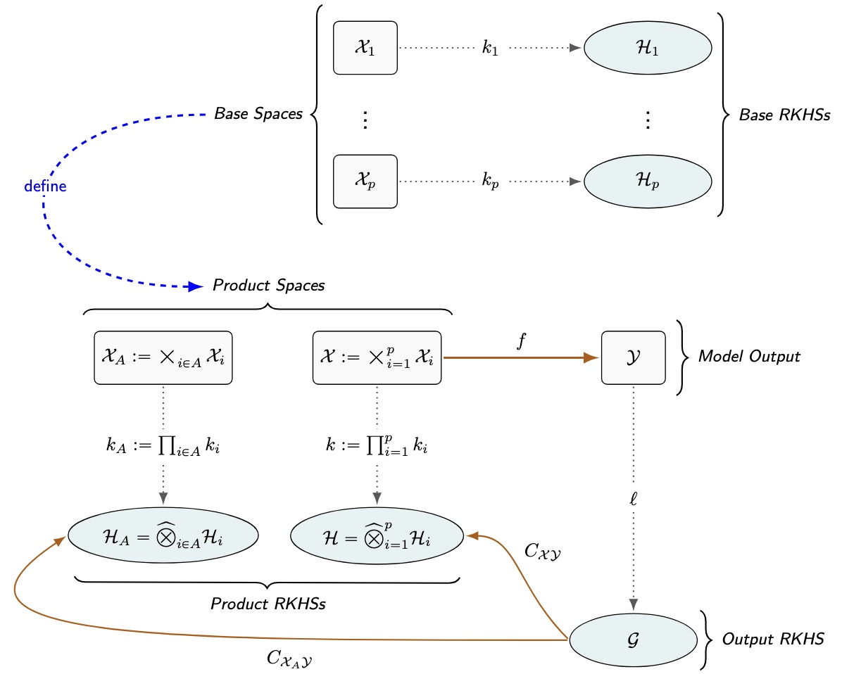
For an index subset $A\subseteq\{1,\dots,p\}$, we define $X_{A}=(X_{i})_{i\in A}$ as a random variable that takes values in the product space $\mathcal{X}_{A}=\prod_{i\in A}\mathcal{X}_{i}$ equipped with the product $\sigma$-algebra $\mathcal{B}(\mathcal{X}_{A})$ and product law $\mathbb{P}_{X_{A}}$. For ease of notation, we omit the brackets from all relevant subscripts when $A=\{i\}$; similarly, we remove the subscripts entirely when $A=\{1,\dots,p\}$. Finally, we equip $\mathcal{X}_{A}$ with a product of characteristic kernels $k_{A}:=\prod_{i\in A}k_{i}$ and $\mathcal{Y}$ with a characteristic kernel $\ell$. We denote the associated RKHSs by $\mathcal{H}_{A}$ and $\mathcal{G}$, respectively. A depiction of the problem setup can be found in Figure 1.

This setup provides the probabilistic foundation for kernel-based sensitivity analysis. A core idea in this context is to construct a cross-covariance operator $C_{X_{A}Y}:\mathcal{G}\to\mathcal{H}_{A}$ given by

(11) $$C_{X_{A}Y} =\int_{\mathcal{X}_{A}\times\mathcal{Y}}(\Phi_{k_{A}}(x)-M_{\mathcal{X}_{A}})\otimes(\Phi_{\ell}(y)-M_{\mathcal{Y}})\ \mathbb{P}_{X_{A},Y}(dx,dy)$$

$$=\int_{\mathcal{X}_{A}\times\mathcal{Y}}\Phi_{\mathcal{X}_{A}}(x)\otimes\Phi_{\mathcal{Y}}(y)\ \mathbb{P}_{X_{A},Y}(dx,dy)-M_{\mathcal{X}_{A}}\otimes M_{\mathcal{Y}},$$

where $\Phi_{X_{A}}$ and $\Phi_{Y}$ are the canonical feature maps of $k_{A}$ and $\ell$, respectively, and $\mathbb{P}_{X_{A},Y}$ denotes the joint law of $(X_{A},Y)$. Under the assumptions of Section 2.3, it is straightforward to show that $C_{X_{A}Y}$ is a Hilbert–Schmidt operator [5].

Figure 1: A depiction of the problem setup.

Definition 2.6.

The Hilbert–Schmidt independence criterion (HSIC) between $X_{A}$ and $Y$ is denoted by $\operatorname{HSIC}(X_{A},Y)$ and defined by the squared Hilbert–Schmidt norm of $C_{X_{A}Y}$; that is,

(12) $$\operatorname{HSIC}(X_{A},Y):=\|C_{X_{A}Y}\|_{HS}^{2}.$$

The authors of [12] use the kernel trick to show that the HSIC between $X_{A}$ and $Y$ can be completely characterized by the kernels endowed upon the spaces $\mathcal{X}_{A}$ and $\mathcal{Y}$. This establishes the HSIC as a kernel-based tool to characterized independence between $X_{A}$ and $Y$, as summarized in the following result:

Theorem 2.7.

Let $k_{A}$ and $\ell$ be characteristic kernels on $\mathcal{X}_{A}$ and $\mathcal{Y}$, respectively. Then,

$$\operatorname{HSIC}(X_{A},Y)=0\quad\text{if and only if}\quad\mathbb{P}_{X_{A},Y}=\mathbb{P}_{X_{A}}\otimes\mathbb{P}_{Y}.$$

When using characteristic kernels, the cross-covariance operator fully encodes the joint distribution, and its vanishing indicates that the joint law factorizes. It follows from Lemma 2.5 that equipping separable Hilbert spaces with Gaussian kernels allows HSIC to generalize the classical idea that zero covariance implies independence. In the following section, we will show that such a setup is not enough to guarantee the monotonicity of the HSIC under marginalization.

3 Monotonicity of the HSIC under marginalization

The discussion in the previous section motivates the use of HSIC as a sensitivity measure. Namely, one may consider the raw HSIC score $\operatorname{HSIC}(X_{A},Y)$ as an indication of the influence of $X_{A}$ upon $Y$. While appealing in its simplicity, the raw HSIC is difficult to interpret. In particular, a large raw HSIC score has no direct interpretation as “influence” of an input. To address this limitation, normalized variants have been proposed. The prevalent approach, suggested in [6], is to use the distance correlation index between $X_{A}$ and $Y$ given by

(13) $$R_{X_{A}}^{2}(Y)\vcentcolon=\frac{\operatorname{HSIC}(X_{A},Y)}{\sqrt{\operatorname{HSIC}(X_{A},X_{A})\operatorname{HSIC}(Y,Y)}}.$$

This rescaling provides a correlation-like interpretation; see [6] for details. Despite their utility, these indices suffer from a lack of a ranking “yardstick” due to the fact that the normalization in (13) depends on $X_{A}$. Furthermore, the definition of the distance correlation indices does not ensure that $R_{X_{i}}^{2}(Y)\leq R_{X_{\{i,j\}}}^{2}(Y)$; that is, the normalization masks how dependence behaves under marginalization.

Without monotonicity under marginalization, we cannot construct analogues of Sobol’ total-effect indices, nor can we interpret HSIC-based indices as fractions of a quantity explaining the contributions of all the inputs to the model output. In what follows, we show how a suitable kernel construction ensures monotonicity. We require that, for $A,B\subseteq\{1,\ldots,p\}$,

$$\operatorname{HSIC}(X_{A},Y)\leq\operatorname{HSIC}(X_{B},Y),\quad\text{whenever}\quad A\subseteq B.$$

When satisfied, this property lays the foundation for defining the total HSIC sensitivity indices (see Section 4.1), which are bounded between 0 and 1 and provide a ranking mechanism to compare the relative importance of parameter subsets.

3.1 Augmented kernel construction

As it will become apparent in the discussion that follows, a critical component of our analysis is that the constant function $\mathbf{1}$ must belong to the RKHS generated from $\mathcal{X}_{i}$ for all $i\in\{1,\dots,p\}$. We also require that the kernels $k_{i}$ defined on $\mathcal{X}_{i}$ are characteristic so that Theorem 2.7 holds.

It is natural to wonder if Gaussian kernels ensure monotonicity under marginalization; however, it is well-established that the RKHS associated with a Gaussian kernel does not contain the constant function $\mathbf{1}$ [30]. We provide a two-part remedy for this issue. With Gaussian kernels in mind as a starting point, we construct a class of augmented kernels that are characteristic on every separable Hilbert space and generate RKHSs that contain the constant function $\mathbf{1}$. We then use the augmented kernels to state and prove Theorem 3.9, the core result of this article, which guarantees monotonicity of the HSIC under marginalization. The following result from [8] informs our kernel construction.

Lemma 3.1 ([8], Proposition 1).

Let $(\mathcal{X},\mathcal{B}(\mathcal{X}),\mathbb{P}_{X})$ be a probability space equipped with kernel $k$. Denote the associated RKHS by $\mathcal{H}$. Then $\mathcal{H}$ admits the orthogonal decomposition

(14) $$\mathcal{H}=\mathcal{H}^{1}\oplus\mathcal{H}^{0},$$

where $\mathcal{H}^{0}$ is an RKHS of zero-mean functions with respect to $\mathbb{P}_{X}$, and $\mathcal{H}^{1}$ is an RKHS with dimension of at most one.

In what follows, we first describe how to transform any given kernel $k$ into one whose associated RKHS consists only of zero-mean functions with respect to $\mathbb{P}_{X}$. We then show that this space $\mathcal{H}^{0}$ does not contain constant functions and demonstrate the orthogonality described in (14) between $\mathcal{H}^{0}$ and $\text{span}\{\mathbf{1}\}$. Finally, we define an augmented kernel as one whose associated RKHS admits the desired decomposition $\mathcal{H}=\text{s}pan\{\mathbf{1}\}\oplus\mathcal{H}^{0}$. We will show that augmented kernels are a correct choice in guaranteeing monotonicity of the HSIC under marginalization.

Definition 3.2.

Let $(\mathcal{X},\mathcal{B}(\mathcal{X}),\mathbb{P}_{X})$ be a probability space and $k:\mathcal{X}\times\mathcal{X}\to\mathbb{R}$ be a kernel. The centering of $k$ with respect to $\mathbb{P}_{X}$ is another kernel $k_{c}:\mathcal{X}\times\mathcal{X}\to\mathbb{R}$ given by

(15) $$k_{c}(x,x^{\prime}):=k(x,x^{\prime})-\int_{\mathcal{X}}k(x,s)\mathbb{P}_{X}(ds)-\int_{\mathcal{X}}k(x^{\prime},s)\mathbb{P}_{X}(ds)+\int_{\mathcal{X}}\int_{\mathcal{X}}k(s,t)\mathbb{P}_{X}(ds)\mathbb{P}_{X}(dt).$$

The following result shows that the canonical feature map associated with $k_{c}$ is mean-zero with respect to $\mathbb{P}_{X}$.

Lemma 3.3.

Let $(\mathcal{X},\mathcal{B}(\mathcal{X}),\mathbb{P}_{X})$ be a probability space and $k:\mathcal{X}\times\mathcal{X}\to\mathbb{R}$ be a kernel. Let $k_{c}$ be the centering of $k$ with respect to $\mathbb{P}_{X}$ and denote by $\Phi_{c}$ the canonical feature map associated with $k_{c}$. Then $\int_{\mathcal{X}}\Phi_{c}(x)\mathbb{P}_{X}(dx)=0$.

Proof 3.4.

We compute directly that

(16) $$\begin{split}\int_{\mathcal{X}}\Phi_{c}(x)&\mathbb{P}_{X}(dx)=\int_{\mathcal{X}}k(x,\cdot)\mathbb{P}_{X}(dx)-\int_{\mathcal{X}}\int_{\mathcal{X}}k(x,s)\mathbb{P}_{X}(ds)\mathbb{P}_{X}(dx)\\ &-\int_{\mathcal{X}}\int_{\mathcal{X}}k(\cdot,s)\mathbb{P}_{X}(ds)\mathbb{P}_{X}(dx)+\int_{\mathcal{X}}\int_{\mathcal{X}}\int_{\mathcal{X}}k(s,t)\mathbb{P}_{X}(ds)\mathbb{P}_{X}(dt)\mathbb{P}_{X}(dx)\end{split}$$

Notice that the integrands of the third and fourth terms in the right-hand side of (16) are independent of $x$. We therefore simplify (16) to read as follows:

(17) $$\begin{split}\int_{\mathcal{X}}\Phi_{c}(x)\mathbb{P}_{X}(dx)=\int_{\mathcal{X}}&k(x,\cdot)\mathbb{P}_{X}(dx)-\int_{\mathcal{X}}\int_{\mathcal{X}}k(x,s)\mathbb{P}_{X}(ds)\mathbb{P}_{X}(dx)\\ &-\int_{\mathcal{X}}k(\cdot,s)\mathbb{P}_{X}(ds)+\int_{\mathcal{X}}\int_{\mathcal{X}}k(s,t)\mathbb{P}_{X}(ds)\mathbb{P}_{X}(dt).\end{split}$$

The second and fourth terms in the right-hand side of (17) are equal due to the symmetry of the kernel function $k$. The first and third terms in this equation are equal by the same property. It follows that

(18) $$\int_{\mathcal{X}}\Phi_{c}(x)\mathbb{P}_{X}(dx)=0,$$

which is the desired conclusion.

With this result in mind, we can use the reproduction property of $k_{c}$ to show that its associated RKHS $\mathcal{H}^{0}$ consists only of mean-zero functions with respect to $\mathbb{P}_{X}$. Indeed, for every $f\in\mathcal{H}^{0}$, we have

(19) $$\int_{\mathcal{X}}f(x)\mathbb{P}_{X}(dx)=\int_{\mathcal{X}}\langle f,\Phi_{c}(x)\rangle_{\mathcal{H}^{0}}\ \mathbb{P}_{X}(dx)=\langle f,\int_{\mathcal{X}}\Phi_{c}(x)\mathbb{P}_{X}(dx)\rangle_{\mathcal{H}^{0}}=\langle f,0\rangle_{\mathcal{H}^{0}}=0,$$

where the penultimate equality follows due to Lemma 3.3. This characterization of functions in $\mathcal{H}^{0}$ allows us to describe the space $\mathcal{H}^{0}$ as the image of $\mathcal{H}_{k}$, the RKHS associated with the original kernel $k$, under a linear operator. Specifically, $\mathcal{H}^{0}=P(\mathcal{H}_{k})$, where

(20) $$Pf\vcentcolon=f-\int_{\mathcal{X}}f(x)\ \mathbb{P}_{X}(dx),\quad f\in\mathcal{H}_{k}.$$

It is straightforward to note that $P^{2}=P$, which yields the interpretation that the centering of $k$ with respect to $\mathbb{P}_{X}$ is a projection of $\mathcal{H}_{k}$ onto the subspace of mean-zero functions with respect to $\mathbb{P}_{X}$. We are particularly interested in the setting where $P$ is injective. Note that

(21) $$\text{ker}P=\{f\in\mathcal{H}_{k}\ |\ f=\int_{\mathcal{X}}f(x)\mathbb{P}_{X}(dx)\}.$$

It follows that $\text{ker}P=\text{span}\{\mathbf{1}\}$ if $\mathbf{1}\in\mathcal{H}_{k}$ and $\text{ker}P=\{0\}$ otherwise. In short, the centering of $k$ with respect to $\mathbb{P}_{X}$ is only bijective when $\mathbf{1}\notin\mathcal{H}$. As such, it is advantageous to consider the centering of Gaussian kernels since their associated RKHSs do not contain $\mathbf{1}$. The following result shows that the characteristic property of these kernels is preserved under centering.

Theorem 3.5.

Let $\mathcal{X}$ be a separable Hilbert space and $k:\mathcal{X}\times\mathcal{X}\to\mathbb{R}$ be a kernel with associated RKHS $\mathcal{H}$. If $\mathbf{1}\notin\mathcal{H}$ and $k$ is characteristic, then $k_{c}$ is characteristic.

Proof 3.6.

Let $\mathcal{H}_{c}$ be the RKHS associated with $k_{c}$, and let $\eta_{k}$ and $\eta_{k_{c}}$ denote the respective KME maps defined with respect to $k$ and $k_{c}$. We know that $\eta_{k}$ is injective since $k$ is characteristic; we will show that $\eta_{k_{c}}$ is injective. First, we observe that every $\mathbb{Q}\in\mathcal{M}(X)$ admits a KME with respect to $k_{c}$ that takes the following form:

(22) $$\eta_{k_{c}}(\mathbb{Q})=\eta_{k}(\mathbb{Q})-\eta_{k}(\mathbb{P}_{X})-\int_{\mathcal{X}}\int_{\mathcal{X}}k(w,s)\mathbb{Q}(dw)\mathbb{P}_{X}(ds)+\int_{\mathcal{X}}\int_{\mathcal{X}}k(s,t)\mathbb{P}_{X}(ds)\mathbb{P}_{X}(dt).$$

To show that $\eta_{k_{c}}$ is injective, suppose that $\mathbb{Q}_{1},\mathbb{Q}_{2}\in\mathcal{M}(\mathcal{X})$ satisfy $\eta_{k_{c}}(\mathbb{Q}_{1})=\eta_{k_{c}}(\mathbb{Q}_{2})$. Substituting (22) into this equality and cancelling like terms yields that

(23) $$\eta_{k}(\mathbb{Q}_{1})-\eta_{k}(\mathbb{Q}_{2})=\int_{\mathcal{X}}\int_{\mathcal{X}}k(w,s)\mathbb{Q}_{1}(dw)\mathbb{P}_{X}(ds)-\int_{\mathcal{X}}\int_{\mathcal{X}}k(w,s)\mathbb{Q}_{2}(dw)\mathbb{P}_{X}(ds).$$

Both terms on the right-hand side of (23) are constants, while both terms on the left-hand side belong to $\mathcal{H}$, the RKHS associated with $k$. As such, we may write that

(24) $$\eta_{k}(\mathbb{Q}_{1})-\eta_{k}(\mathbb{Q}_{2})=c\cdot\mathbf{1}$$

for some constant $c\in\mathbb{R}$. But since $\mathbf{1}\notin\mathcal{H}$, we conclude that $c=0$. Then $\eta_{k}(\mathbb{Q}_{1})=\eta_{k}(\mathbb{Q}_{2})$, and so the injectivity of $\eta_{k}$ yields $\mathbb{Q}_{1}=\mathbb{Q}_{2}$ as desired.

Finally, we describe how to construct an RKHS $\mathcal{H}=\text{span}\{\mathbf{1}\}\oplus\mathcal{H}^{0}$ as in Lemma 14 whose reproducing kernel is characteristic on every separable Hilbert space. While the “base kernel” $k$ may be any characteristic kernel whose associated RKHS does not contain the constant function $\mathbf{1}$, it is advantageous to use the Gaussian kernels for convenience.

Corollary 3.7.

Let $\mathcal{X}$ be a separable Hilbert space and $k:\mathcal{X}\times\mathcal{X}\to\mathbb{R}$ be a kernel with associated RKHS $\mathcal{H}$. If $\mathbf{1}\notin\mathcal{H}$ and $k$ is characteristic, then the kernel $k^{*}:\mathcal{X}\times\mathcal{X}\to\mathbb{R}$ defined by $k^{*}(x,x^{\prime}):=1+k_{c}(x,x^{\prime})$ is also characteristic.

Proof 3.8.

Denote by $\eta^{*}$ and $\eta_{c}$ the KME maps defined with respect to $k^{*}$ and $k_{c}$, respectively. Suppose that $\mathbb{Q}_{1},\mathbb{Q}_{2}\in\mathcal{M}(\mathcal{X})$ satisfy $\eta^{*}(\mathbb{Q}_{1})=\eta^{*}(\mathbb{Q}_{2})$. It is straightforward to compute that

(25) $$\eta^{*}(\mathbb{Q}_{1})-\eta^{*}(\mathbb{Q}_{2})=\eta_{c}(\mathbb{Q}_{1})-\eta_{c}(\mathbb{Q}_{2})=0.$$

Hence, since $\mathbf{1}\notin\mathcal{H}$, we have $\mathbb{Q}_{1}=\mathbb{Q}_{2}$ by Theorem 3.5.

We refer to kernels of the form described in Corollary 3.7 as augmented kernels, although other authors use the term ANOVA kernels due to their role in defining a functional ANOVA decomposition under the assumption of independent inputs [7, 8]. Our choice in nomenclature is made to highlight the lack of assumptions we impose on the dependence of inputs.

3.2 Ensuring monotonicity

With the developments in the previous subsection in place, we are now ready to state and prove Theorem 3.9, which is the core result of this article. This result shows that, by using augmented kernels, we can ensure the monotonicity of the HSIC under marginalization.

Theorem 3.9.

Given the setup of Section 2.3, assume that $k_{\ell}$ is an augmented kernel for each $\ell\in\{1,\ldots,p\}$. Then for every $A\subseteq B\subseteq\{1,\dots,p\}$, we have

(26) $$\operatorname{HSIC}(X_{A},Y)\leq\operatorname{HSIC}(X_{B},Y).$$

Proof 3.10.

Without loss of generality, we assume that $B=\{1,\dots,p\}$. Also, since the conclusion of the theorem holds trivially when $A=B$, we assume $A$ is a proper subset of $B$. We consider $\mathcal{H}=\mathcal{H}_{A}\widehat{\otimes}\mathcal{H}_{A^{c}}$ and define $\mathbf{1}_{A^{c}}\in\mathcal{H}_{A^{c}}$ so that $\mathbf{1}_{A^{c}}=\mathbf{1}\otimes\dots\otimes\mathbf{1}$ is the tensor product of $p-|A|$ copies of $\mathbf{1}$. Note that since the RKHSs associated with augmented kernels contain the constant function $\mathbf{1}$ (cf. Corollary 3.7), we know that $\mathbf{1}_{A^{c}}$ is well-defined. Define $i:\mathcal{H}_{A}\to\mathcal{H}$ so that $i(f_{A})=f_{A}\otimes\mathbf{1}_{A^{c}}$ for every $f_{A}\in\mathcal{H}_{A}$. It is straightforward to show that $i$ is a bounded linear operator with operator norm equal to 1. The adjoint $i^{*}$ of $i$ is therefore a bounded linear operator with the same norm.

We now claim that $C_{X_{A}Y}=i^{*}C_{XY}$. It suffices to show that for every $f_{A}\in\mathcal{H}_{A}$ and $g\in\mathcal{G}$,

(27) $$\langle f_{A},C_{X_{A}Y}(g)\rangle_{\mathcal{H}_{A}}=\langle f_{A},i^{*}C_{XY}(g)\rangle_{\mathcal{H}_{A}}.$$

Recalling (11) and applying the kernel trick to the left-hand side of Eq. 27 yields

(28) $$\begin{split}\langle f_{A},C_{X_{A}Y}(g)\rangle_{\mathcal{H}_{A}}&=\int_{\mathcal{X}_{A}\times\mathcal{Y}}f_{A}(x_{A})g(y)\mathbb{P}_{X_{A}\times Y}(dx_{A},dy)\\ &\quad\quad-\int_{\mathcal{X}_{A}}f_{A}(x_{A})\mathbb{P}_{X_{A}}(dx_{A})\int_{\mathcal{Y}}g(y)\mathbb{P}_{Y}(dy).\end{split}$$

Considering the right-hand side of Eq. 27, we note

(29) $$\langle f_{A},i^{*}C_{XY}(g)\rangle_{\mathcal{H}_{A}}=\langle i(f_{A}),C_{XY}(g)\rangle_{\mathcal{H}_{A}}.$$

After applying the kernel trick and Fubini’s Theorem to Eq. 29, we obtain

(30) $$\begin{split}\langle i(f_{A}),C_{XY}(g)\rangle_{\mathcal{H}_{A}}&=\int_{\mathcal{X}_{A}\times\mathcal{Y}}f_{A}(x_{A})g(y)\mathbb{P}_{X_{A}\times Y}(dx_{A},dy)\\ &\quad\quad-\int_{\mathcal{X}_{A}}f_{A}(x_{A})\mathbb{P}_{X_{A}}(dx_{A})\int_{\mathcal{Y}}g(y)\mathbb{P}_{Y}(dy),\end{split}$$

which is precisely Eq. 28. It follows that $C_{X_{A}Y}=i^{*}C_{XY}$. Moreover, we have that

(31) $$\|C_{X_{A}Y}\|_{HS}=\|i^{*}C_{XY}\|_{HS}\leq\|C_{XY}\|_{HS}$$

due to the submultiplicativity of the Hilbert–Schmidt norm under compositions with bounded linear operators. Squaring both sides of Eq. 31 yields that $\operatorname{HSIC}(X_{A},Y)\leq\operatorname{HSIC}(X,Y)$.

4 The total HSIC sensitivity index

In this section, we use the setting of Theorem 3.9 to define the total HSIC sensitivity index. We also discuss efficient methods for computing these indices.

4.1 Defining the total HSIC sensitivity index

Let $A\subseteq\{1,\dots,p\}$. Given the setup prescribed by Section 2.3 and assuming that all kernels therein are (products of) augmented kernels, we define the Total HSIC sensitivity index as

(32) $$\mathbb{T}_{A}(f):=1-\frac{\operatorname{HSIC}(X_{\sim A},Y)}{\operatorname{HSIC}(X,Y)},$$

where $X_{\sim A}=(X_{i})_{i\notin A}$. For ease of notation, we write $\mathbb{T}_{i}(f)$ whenever $A=\{i\}$. This definition mirrors the structure of the total-effect Sobol’ index, but quantifies much more of the distributional dependence between $X_{A}$ and $Y$ than variance alone. We note that the collection of total HSIC sensitivity indices does not form an additive decomposition: the sum of $\mathbb{T}_{A}(f)$ over all index subsets $A$ need not equal 1. This is not a defect, but a reflection of the fact that $\mathbb{T}_{A}(f)$ captures all the effects of $X_{A}$ upon $Y$ in a manner analogous to total-effect Sobol’ indices. Since our setup does not require independence of the inputs, the total HSIC indices capture the first-order, joint, and correlation-based influence of a parameter subset upon the model output. Like the Sobol’ indices, total HSIC sensitivity indices measure a “share” of influence, but now in broader generality.

The index $\mathbb{T}_{A}(f)$ admits two natural interpretations: (1) the share of $\operatorname{HSIC}(X,Y)$ that can be attributed to the subset $X_{A}$; and (2) the relative error incurred by approximating $\operatorname{HSIC}(X,Y)$ when $X_{A}$ is excluded from the input set. In contrast to the raw HSIC and distance correlation indices, the total HSIC sensitivity indices do not suffer from the yardstick issue due to monotonicity under marginalization. Indeed, considering the effects of additional parameters upon the model output will only increase the corresponding sensitivity index. The following result demonstrates that the total HSIC sensitivity indices are bounded between 0 and 1, a key property not exhibited by the total-effect Sobol’ indices under the assumption of arbitrarily-correlated inputs [13].

Lemma 4.1.

If the setup in Section 2.3 is satisfied and all kernels therein are (products of) augmented kernels, then $0\leq\mathbb{T}_{i}(f)\leq 1$.

Proof 4.2.

Immediately follows from the monotonicity of HSIC under marginalization.

In summary, the total HSIC sensitivity index unifies the strengths of existing methods: it preserves the generality and computational efficiency of the raw HSIC, while recovering the interpretability that make Sobol’ indices so useful in practice. As such, the index $\mathbb{T}_{A}(f)$ provides a compelling candidate for robust sensitivity analysis across a wide variety of models. In the following section, we describe how to estimate the HSIC and total HSIC sensitivity indices from data, and then present numerical experiments comparing distance correlation, total HSIC, and total-effect Sobol’ indices in practice.

4.2 Computing the total HSIC sensitivity index

We now turn to the numerical estimation of the total HSIC sensitivity indices defined in the previous section. Throughout the remainder of the article, we employ the augmented kernels prescribed in Section 4.2, which were chosen to ensure that the indices satisfy monotonicity under marginalization and are characteristic on every separable Hilbert space. In particular, we choose Gaussian kernels as the base from which we obtain the augmented kernels described in Corollary 3.7. For each index subset $A\subset\{1,\dots,p\}$, we select the bandwidth parameter $\sigma_{X_{A}}$ for the Gaussian kernel $k_{\sigma_{X_{A}}}$ according to the sample-based median heuristic given by

(33) $$\sigma_{X}=\mathrm{median}\{\|X_{A}^{(i)}-X_{A}^{(j)}\|_{\mathcal{X}_{A}}\ |\ {i<j}\},$$

computed over all pairwise distances among the samples. This heuristic provides a convenient baseline that adapts to the spread of the data and generally yields stable estimates near its chosen scale. As we demonstrate in the discussions to follow, this choice is sufficient for obtaining consistent rankings of parameter importance in the test problems considered. Having addressed the issue of kernel selection, we turn our attention now to the empirical estimator for the HSIC.

Given $n$ independent realizations $(X^{(j)},Y^{(j)})_{j=1}^{n}$ from the joint law of the model inputs and output, the well-known empirical estimator for the HSIC presented in [12] takes the form

(34) $$\widehat{\operatorname{HSIC}}(X,Y)=\frac{1}{n^{2}}\operatorname{tr}(\mathbf{KHLH}),$$

where $\mathbf{K,L}\in\mathbb{R}^{n\times n}$ are Gram matrices whose elements are respectively given by

$$K_{ij}:=k(X^{(i)},X^{(j)})\quad\text{and}\quad L_{ij}:=\ell(Y^{(i)},Y^{(j)}).$$

The matrix $\mathbf{H}$ centers the data and takes the form

$$\mathbf{H}:=\mathbf{I}_{n}-\mathbf{zz}^{T},$$

where $\mathbf{z}=\frac{1}{\sqrt{n}}\mathbf{1}_{n}$. An estimator for $\operatorname{HSIC}(X_{A},Y)$ is defined analogously, using $k_{A}$ in place of $k$ for the entries of $\mathbf{K}$. This matrix formulation highlights the computational structure of the estimator: once $\mathbf{K}$ and $\mathbf{L}$ are formed, $\widehat{\mathrm{HSIC}}$ reduces to a single trace operation.

Direct computation of the estimate in Eq. 34 involves an $\mathcal{O}(n^{3})$ matrix product, which becomes computationally prohibitive for large sample sizes $n$. To achieve an $\mathcal{O}(n^{2})$ complexity, the trace can be re-expressed into a simplified component-wise summation. This procedure avoids multiplication with the centering matrix $\mathbf{H}$, resulting in a faster calculation suitable for large-scale applications. The following result underpins our improved calculation.

Lemma 4.3.

Let $\mathbf{z}=\frac{1}{\sqrt{n}}\mathbf{1}_{n}$. We obtain the following identity:

$$\operatorname{tr}(\mathbf{KHLH})=\operatorname{tr}(\mathbf{KL})-2\langle\mathbf{Kz},\mathbf{Lz}\rangle_{2}+\langle\mathbf{z},\mathbf{Kz}\rangle_{2}\langle\mathbf{z},\mathbf{Lz}\rangle_{2},$$

where $\langle\cdot,\cdot\rangle_{2}$ denotes the Euclidean inner product in $\mathbb{R}^{n}$.

Proof 4.4.

This identity is a routine calculation using the cyclic property of the trace.

Using this result, we can outline a simple procedure for empirically estimating the HSIC. Letting $\mathbf{K}^{(i)}$ denote the $i^{\text{th}}$ column of $\mathbf{K}$ and using an analogous notation for the columns of $\mathbf{L}$, we make two key observations. First, we recall that $\mathbf{K}$ and $\mathbf{L}$ are symmetric real-valued matrices, and so $\mathbf{K}^{(i)}$ and $\mathbf{L}^{(i)}$ are the same as the $i^{\text{th}}$ rows of the respective matrices. Second, we note that the $i^{\text{th}}$ row sum of $\mathbf{K}$ is equal to the $i^{\text{th}}$ element of $\mathbf{K1}_{n}$; that is,

(35) $$[\mathbf{K1}_{n}]_{i}=\sum_{j=1}^{n}K_{ij}.$$

An analogous identity holds for $\mathbf{L}$. With these remarks in mind, the Algorithm 1 describes a procedure that requires only matrix-vector products with $\mathbf{K}$ and $\mathbf{L}$. There is no need to form any matrix products.

Algorithm 1 Efficient Computation of HSIC Estimator

1:Set $S=0$

2:for $i=1,\ldots,n$ do

3:  $\mathbf{a}=\mathbf{K}^{(i)}$

4:  $\mathbf{b}=\mathbf{L}^{(i)}$

5:  $S=S+\langle\mathbf{a},\mathbf{b}\rangle_{2}$

6:  $u_{i}=\langle\mathbf{a},\mathbf{z}\rangle_{2}$

7:  $v_{i}=\langle\mathbf{b},\mathbf{z}\rangle_{2}$

8:end for

9:Return $\widehat{\operatorname{HSIC}}=\frac{1}{n^{2}}[S-2\langle\mathbf{u},\mathbf{v}\rangle_{2}+\langle\mathbf{u},\mathbf{z}\rangle_{2}\langle\mathbf{v},\mathbf{z}\rangle_{2}]$.

This procedure only requires that we store one column of the matrices $\mathbf{K}$ and $\mathbf{L}$ at a time, thereby reducing the storage requirement from $\mathcal{O}(n^{2})$ to $\mathcal{O}(n)$. Furthermore, Algorithm 1 describes a single-loop Monte Carlo estimator, which significantly out-performs the double-loop Monte Carlo estimators typically employed in variance-based sensitivity analysis.

The empirical estimator for the HSIC underpins our definition of an empirical estimator for the total HSIC sensitivity indices. For each input subset $A\subseteq\{1,\dots,p\}$, the empirical estimator for $\mathbb{T}_{A}(f)$ is given by

(36) $$\widehat{\mathbb{T}}_{A}(f):=1-\frac{\widehat{\operatorname{HSIC}}(X_{\sim A},Y)}{\widehat{\operatorname{HSIC}}(X,Y)}.$$

This estimator converges to the population value at rate $\mathcal{O}(n^{-1/2})$, and its bias is of order $\mathcal{O}(n^{-1})$ [11]. In practice, these asymptotic properties translate into smooth convergence of the estimated indices as $n$ increases. While an unbiased estimator for the HSIC has been presented [7, 12], the convenient expression given by Eq. 34 is preferred for the scope of our study. In the following section, we implement the estimator for total HSIC sensitivity indices in several illustrative numerical experiments.

5 Numerical Experiments

In this section, we demonstrate the utility of the total HSIC sensitivity indices with three numerical experiments. We first consider the Ishigami function, a common example of a model with independent inputs and a scalar output. The total-effect Sobol’ indices for this model are known analytically, and we demonstrate that the total HSIC sensitivity indices provide a ranking of parameter influence that is consistent with these values. Next, we present a portfolio model whose output remains scalar-valued, but whose inputs obey a nontrivial correlation structure. We demonstrate that, in this case, the total HSIC sensitivity indices provide a more accurate and interpretable ranking of parameter influence than the total-effect Sobol’ indices for models with correlated inputs proposed by [13]. Finally, we conclude our analysis by examining a model that describes the spread of cholera over the course of 300 weeks. The model response is functional-valued in this example, and we demonstrate that the resulting total HSIC sensitivity indices vary noticeably depending upon the assumed correlation structure of the inputs. We use this fact to justify the consideration of parameter correlations in real-world models, especially in the context of model reduction.

5.1 Ishigami function

To illustrate the practical computation of HSIC-based sensitivity indices, we consider the Ishigami function, a classical nonlinear test problem defined as

(37) $$f(x_{1},x_{2},x_{3})=\sin(x_{1})+a\,\sin^{2}(x_{2})+b\,x_{3}^{4}\sin(x_{1}),$$

where $a=5$, $b=0.1$, and the inputs $X_{i}\sim\mathcal{U}(-\pi,\pi)$ are mutually independent. This model is well-known for its strong nonlinearity and interaction effects: $X_{3}$ influences the output only through its interaction with $X_{1}$, while the contributions of $X_{2}$ are independent of any interactions with the other inputs.

(a) $\mathbb{T}_{1}(f)$

(b) $\mathbb{T}_{2}(f)$

(c) $\mathbb{T}_{3}(f)$

Figure 2: Estimated total HSIC sensitivity indices as functions of sample size $n$.

To assess sampling adequacy, Figure 2 depicts the estimates $\widehat{\mathbb{T}}_{i}(f)$ as a function of the sample size. The estimates stabilize after around $n=700$ samples, indicating that any larger choice of $n$ provides sufficient accuracy for all three input parameters. Given this analysis, we draw $n=1,000$ independent samples of $(X_{1},X_{2},X_{3})$ and evaluate $Y=f(X_{1},X_{2},X_{3})$. For each input $X_{i}$, total HSIC indices $\widehat{\mathbb{T}}_{i}$ are computed using the estimator in Eq. 36 with the kernels as prescribed in Section 4.2 and bandwidths determined by the median heuristic Eq. 33. Distance correlation indices and total-effect Sobol’ indices $S_{i}^{T}$ are also computed for comparison. Figure 3 depicts the resulting indices.

Figure 3 demonstrates that the total HSIC sensitivity indices provide a consistent parameter influence ranking with that obtained from the total-effect Sobol’ indices. This agreement reflects the fact that, under independent inputs, the two measures capture similar notions of variable importance: Sobol’ indices quantify contributions to output variance, whereas HSIC detects general statistical dependence. Discrepancies between their magnitudes, particularly between $\mathbb{T}_{2}$ and $S_{2}^{T}$, are attributable to the moment-independence of HSIC, which quantifies dependence structures beyond second-order moments.

The distance correlation indices reproduce the same ranking of influential parameters ($X_{1}$ dominant, followed by $X_{3}$ and $X_{2}$), but their magnitudes differ substantially due to normalization differences inherent to the metric. Overall, the comparison highlights that HSIC-based total indices retain the interpretability of variance-based measures while extending sensitivity analysis to higher-order dependencies. In the next example, we investigate the performance of the total HSIC sensitivity indices for a model whose inputs are assumed to be dependent.

(a) Distance Correlation Indices

(b) Total HSIC Indices

(c) Total-effect Sobol’ Indices

Figure 3: A comparison of sensitivity indices for the Ishigami function.

5.2 Correlated portfolio model

In this example, we illustrate how total HSIC sensitivity indices behave when the assumption of parameter independence is removed. We examine a model that was first considered in [13] for their study of Sobol’ indices for models with correlated inputs. The model is defined by

(38) $$Y=20X_{1}+16X_{2}+12X_{3}+10X_{4}+4X_{5},$$

where $X=[X_{1},\dots,X_{5}]$ follows a multivariate normal distribution $\mathcal{N}(\mu,\Sigma)$ with mean vector $\mu$ and covariance matrix $\Sigma$ given by

(39) $$\mu=\begin{bmatrix}0\\ 0\\ 0\\ 0\\ 0\end{bmatrix},\qquad\Sigma=\begin{bmatrix}1&0.5\rho&0.5\rho&0&0.8\rho\\ 0.5\rho&1&0&0&0\\ 0.5\rho&0&1&0&0.3\rho\\ 0&0&0&1&0\\ 0.8\rho&0&0.3\rho&0&1\end{bmatrix}.$$

In this example, $\rho\in[0,1]$ controls the strength of correlation among subsets of the inputs. It was noted in [13, Figure 1] that as $\rho$ increases toward $1$, the indices corresponding to the four correlated parameters collapse and the only uncorrelated variable, $X_{4}$, appears to be dominant. The authors explain this behavior as follows: when correlations between parameters are strengthened, the influence of one variable upon the output may be approximated by the other variables. This phenomenon does not exist in the case of independent inputs, but explains why the total-effect Sobol’ indices are decreasing in $\rho$ for all parameters except for $X_{4}$. Despite this explanation, we demonstrate that Sobol’ analysis fails to provide an accurate parameter ranking in the case of correlated inputs, when the goal is model reduction by fixing non-influential parameters.

(a) Distance Correlation Indices

(b) Total HSIC Indices

Figure 4: Sensitivity indices for the correlated portfolio model as functions of $\rho$.

We compute distance correlation and total HSIC sensitivity indices for the correlation values $\rho_{j}=j/20$ for $j=0,\dots,20$, using $n=2,000$ samples per computation. The resulting indices are plotted in Figure 4 as functions of $\rho$. Unlike the Sobol’ or distance correlation indices, the total HSIC indices remain stable across increasing correlation. The ranking of influential variables is preserved for all $\rho$: $X_{1}$ remains most influential, while $X_{5}$ gradually gains importance as its correlations with the dominant variables strengthen. At the high-correlation extreme ($\rho\approx 1$), total HSIC indices indicate that $X_{5}$ surpasses $X_{4}$ and $X_{3}$ in importance, consistent with the model structure. It should be noted that the distance correlation and total HSIC sensitivity indices provide the same parameter rankings; however, the magnitudes of these indices are only interpretable in the case of total HSIC.

To qualitatively validate these findings, we performed parameter dimension reduction at $\rho=0$ and $\rho=1$ by fixing the least influential parameter ($X_{5}$ and $X_{4}$, respectively, as indicated by Figure 4) at its mean value. We compare the resulting conditional output distribution to that of the full model using $n=1\times 10^{7}$ Monte Carlo samples. As shown in Figure 5, the reduced and full output distributions agree closely in both cases, supporting the conclusion that total HSIC sensitivity indices correctly identify parameters whose variation can be neglected without materially affecting the model response.

(a) $\rho=0$

(b) $\rho=1$

Figure 5: Model reduction informed by Figure 4 at different values of $\rho$.

Figure 6: Model reduction informed by the approach in [13] at $\rho=1$.

We also used this method to demonstrate the limitations of the total-effect Sobol’ indices for parameter dimension reduction. Indeed, [13] suggests that $X_{5}$ holds minimal influence over the model output when $\rho=1$. This may suggest $X_{5}$ as a candidate to be fixed at its mean value for the purpose of dimension reduction. We compare the conditional output distribution to that of the full model using $n=1\times 10^{7}$ Monte Carlo samples in Figure 6. The significant discrepancy between the distributions suggests that $X_{5}$ holds more influence over the model than the Sobol’ indices describe, further demonstrating the advantage of total HSIC sensitivity indices over variance-based sensitivity measures.

Overall, this example demonstrates that total HSIC indices preserve interpretability and ranking consistency under correlated inputs. They correctly identify parameter importance without being misled by shared variability, offering a principled and robust alternative to variance-based sensitivity measures.

5.3 Function-valued cholera model

As a final example, we apply the total HSIC framework to a model with correlated inputs and a function-valued output. Specifically, we consider the nonlinear epidemiological model of cholera transmission introduced in [14] and studied in [1, 4]. This model describes the coupled dynamics between the human population and two environmental bacterial reservoirs, capturing both direct and indirect infection pathways. The objective is to quantify the sensitivity of the infected population $I(t)$ to uncertainties in the epidemiological parameters, and to evaluate whether HSIC-based indices remain robust in this biologically realistic, correlated-input setting.

The population is divided into susceptible ($S$), infectious ($I$), and recovered ($R$) compartments, and the environmental bacteria are split into highly infectious ($B_{H}$) and lowly infectious ($B_{L}$) concentrations. The state vector $y=(S,I,R,B_{H},B_{L})^{\top}\in\mathbb{R}^{5}$ evolves according to

$$\begin{split}\frac{dS}{dt}&=bN_{\mathrm{pop}}-\beta_{L}S\frac{B_{L}}{\kappa_{L}+B_{L}}-\beta_{H}S\frac{B_{H}}{\kappa_{H}+B_{H}}-bS,\\[2.0pt] \frac{dI}{dt}&=\beta_{L}S\frac{B_{L}}{\kappa_{L}+B_{L}}+\beta_{H}S\frac{B_{H}}{\kappa_{H}+B_{H}}-(\gamma+b)I,\\[2.0pt] \frac{dR}{dt}&=\gamma I-bR,\\[2.0pt] \frac{dB_{H}}{dt}&=\xi I-\chi B_{H},\\[2.0pt] \frac{dB_{L}}{dt}&=\chi B_{H}-\delta B_{L}.\end{split}$$

Initial conditions are given by $(S(0),I(0),R(0),B_{H}(0),B_{L}(0))=(N_{\mathrm{pop}}-1,1,0,0,0)$, with $N_{\mathrm{pop}}=10,000$, and the system is solved up to $T=300$ weeks using MATLAB’s ode45 solver. The model parameters, along with their units and nominal values adopted from [4, 14], are summarized in Table 1.

Parameter	Description	Units	Nominal value
$\beta_{L}$	Rate of drinking low-infectious cholera	week-1	1.5
$\beta_{H}$	Rate of drinking high-infectious cholera	week-1	7.5
$\kappa_{L}$	$B_{L}$ cholera carrying capacity	bacteria·mL-1	$10^{6}$
$\kappa_{H}$	$B_{H}$ cholera carrying capacity	bacteria·mL-1	$7\times 10^{8}$
$b$	Human birth/death rate	week-1	$1/1560$
$\chi$	Decay rate from $B_{H}$ to $B_{L}$	week-1	1/168
$\xi$	$B_{H}$ water contamination rate	$\frac{\text{bacteria\textperiodcentered mL${}^{-1}$}}{\text{individual\textperiodcentered week}}$	70
$\delta$	Death rate of $B_{L}$ cholera	week-1	7/30
$\gamma$	Recovery rate from cholera	week-1	7/5

Table 1: Nominal cholera model parameters from [14, 4].

We simulate a realistic study by obtaining a data-informed estimate of parameter correlations. As described in great detail by [25], we perform an ordinary least squares (OLS) fit of the model to synthetic data to obtain estimates of the mean parameter vector and corresponding empirical correlation matrix. The correlation structure, depicted in Figure 7, reveals strong dependencies among the transmission and bacterial parameters, particularly $(\beta_{H},\beta_{L})$ and $(\xi,\chi)$, corresponding to shared infection and decay processes.

The quantity of interest is the infected population $I(t)$ over $t\in[0,300]$. We compute the total HSIC indices for each parameter using $n=1,500$ samples drawn from the multivariate normal distribution with mean vector and covariance matrix obtained through the OLS estimates computed above. As a comparison, we also compute the total HSIC indices using $n=1,500$ samples drawn from independent uniform distributions with bounds determined by $\pm 10\%$ of the mean vector determined by the OLS estimate. The subsequent indices vary significantly, and the results are displayed in Figure 8.

Figure 7: Empirical parameter correlation matrix obtained from OLS estimation. Strong correlations occur between parameters governing infection and bacterial dynamics.

(a) Independent uniform sampling

(b) Multivariate normal sampling

Figure 8: A comparison of total HSIC indices under the assumptions of independent (Figure 8(a)) and correlated (Figure 8(b)) parameters.

Figure 9: Relative error between the full and reduced posterior distributions of $I(t)$ after fixing the least-influential parameter $b$ at its OLS mean value. The small discrepancy confirms the accuracy of HSIC-guided model reduction.

Both sets of total HSIC indices identify $\beta_{H}$ as significantly influencing the infection curve $I(t)$. Similarly, both sets of indices capture the minimal effects of $b$ upon the model output. The remaining parameters’ influence varies significantly between the assumptions of independent and correlated inputs, reinforcing our claim that the parameter correlation structure should not be neglected when performing sensitivity analysis. In particular, the correlation structure greatly influences the feasibility of parameter dimension reduction based on the HSIC results. Under the assumption of correlated inputs, $b$ appears as the least influential parameter. We therefore fix $b$ at its OLS mean value and generate the full and reduced distributions of the model output using $n=1\times 10^{6}$ Monte Carlo samples. Figure 9 shows the relative error between the mean curves of the full and reduced distributions of $I(t)$, demonstrating that fixing $b$ introduces negligible error. This result supports the exclusion of $b$ from the model for simplified inference. Overall, this experiment demonstrates that total HSIC indices extend naturally to time-dependent and correlated epidemiological models, yielding interpretable and stable sensitivity rankings that can guide principled model simplification.

6 Conclusions

The augmented kernel construction presented in this work guarantees the property of monotonicity under marginalization for HSIC-based sensitivity analysis. Under this framework, the total HSIC sensitivity indices accommodate a wide variety of parameter types, are interpretable as a share of total influence over the model output, and require no assumptions of independence among the inputs. Our numerical experiments demonstrate that the total HSIC sensitivity index correctly identifies non-influential parameters in the presence of strong statistical dependence among inputs. As such, the total HSIC sensitivity indices can serve as a flexible tool in parameter dimension reduction by fixing non-influential parameters at their nominal values.

The present study motivates several interesting lines of inquiry for future work. For example, it would be desirable to derive more computationally efficient estimators to improve scalability in high-dimensional settings This could also involve use of efficient surrogate models to relieve the sampling procedure from potentially expensive model evaluations. Furthermore, we plan to investigate the decomposition of total HSIC indices into component terms to achieve an attribution of influence analogous to the HSIC-ANOVA decomposition, but without the assumption of parameter independence.

References

- [1] A. Alexanderian, P. Gremaud, and R. C. Smith, Variance-based sensitivity analysis for time-dependent processes, Reliability Engineering & System Safety, 196 (2020), p. 106722.
- [2] N. Aronszajn, Theory of reproducing kernels, Transactions of the American Mathematical Society, 68 (1950), pp. 337–404.
- [3] J. Barr and H. Rabitz, A generalized kernel method for global sensitivity analysis, SIAM/ASA J. Uncertainty Quantification, 10 (2022), pp. 27–54.
- [4] H. L. Cleaves, A. Alexanderian, H. Guy, R. C. Smith, and M. Yu, Derivative-based global sensitivity analysis for models with high-dimensional inputs and functional outputs, SIAM Journal on Scientific Computing, 41 (2019), pp. A3524–A3551.
- [5] G. da Prato, An introduction to infinite-dimensional analysis, Springer, 2006.
- [6] S. da Veiga, Global sensitivity analysis with dependence measures, Journal of Statistical Computation and Simulation, 85 (2015), pp. 1283–1305.
- [7] S. da Veiga, Kernel-based ANOVA decomposition and Shapley effects – application to global sensitivity analysis, arXiv preprint arXiv:2101.05487, (2021).
- [8] N. Durrande, D. Ginsbourger, O. Roustant, and L. Carraro, ANOVA kernels and RKHS of zero mean functions for model-based sensitivity analysis, Journal of Multivariate Analysis, 115 (2011), pp. 57–67.
- [9] F. Gamboa, A. Janon, T. Klein, and A. Lagnoux, Sensitivity analysis for multidimensional and functional outputs, Electronic Journal of Statistics, 8 (2014), pp. 575–603.
- [10] D. Greenfeld and U. Shalit, Robust learning with the Hilbert-Schmidt Independence Criterion, in Proceedings of the 37th International Conference on Machine Learning, vol. 119, Proceedings of Machine Learning Research, 2020, pp. 3759–3768.
- [11] A. Gretton, O. Bousquet, A. Smola, and B. Schölkopf, Measuring statistical dependence with Hilbert-Schmidt norms, in Algorithmic Learning Theory, S. Jain, H. U. Simon, and E. Tomita, eds., Springer Berlin Heidelberg, 2005, pp. 63–77.
- [12] A. Gretton, R. Herbrich, A. Smola, O. Bousquet, and B. Schölkopf, Kernel methods for measuring independence, Journal of Machine Learning Research, 6 (2005), pp. 2075–2129.
- [13] J. L. Hart and P. Gremaud, An approximation theoretic perspective of Sobol’ indices with dependent variables, International Journal of Uncertainty Quantification, 8 (2018), pp. 483–493.
- [14] D. M. Hartley, J. G. J. Morris, and D. L. Smith, Hyperinfectivity: a critical element in the ability of v. cholerae to cause epidemics?, PLoS medicine, (2005).
- [15] M. Hein and O. Bousquet, Kernels, associated structures, and generalizations, Tech. Report 127, Max Planck Institute for Biological Cybernetics, 2004.
- [16] B. Iooss and C. Prieur, Shapley effects for sensitivity analysis with correlated inputs: Comparisons with Sobol’ indices, numerical estimation and applications, International Journal for Uncertainty Quantification, 9 (2019), pp. 493–514.
- [17] S. Kucherenko and B. Iooss, Derivative-based global sensitivity measures, Handbook of Uncertainty Quantification, (2017).
- [18] S. Kucherenko, S. Tarantola, and P. Annoni, Estimation of global sensitivity indices for models with dependent variables, Computer Physics Communications, 183 (2012), pp. 937–946.
- [19] M. Lamboni and S. Kucherenko, Multivariate sensitivity analysis and derivative-based global sensitivity measures with dependent variables, Reliability Engineering & System Safety, 212 (2021), p. 107519.
- [20] G. Li, H. Rabitz, P. E. Yelvington, O. O. Oluwole, F. Bacon, C. E. Kolb, and J. Schoendorf, Global sensitivity analysis for systems with independent and/or correlated inputs, The Journal of Physical Chemistry A, 114 (2010), pp. 6022–6032.
- [21] C. A. Micchelli, Y. Xu, and H. Zhang, Universal kernels, Journal of Machine Learning Research, 7 (2006), pp. 2651–2667.
- [22] K. Muandet, K. Fukumizu, B. Sriperumbudur, and B. Sch olkopf, Kernel mean embedding of distributions: A review and beyond, Foundations and Trends® in Machine Learning, 1-2 (2017), pp. 1–141.
- [23] V. I. Paulsen and M. Raghupathi, An introduction to the theory of reproducing kernel Hilbert spaces, Cambridge University Press, 2016.
- [24] H. Rabitz, Global sensitivity analysis for systems with independent and/or correlated inputs, Procedia - Social and Behavioral Sciences, 2 (2010), pp. 7587–7589. Sixth International Conference on Sensitivity Analysis of Model Output.
- [25] R. C. Smith, Uncertainty Quantification: theory, implementation, and applications, vol. 12, SIAM, 2013.
- [26] I. M. Sobol’, Global sensitivity indices for nonlinear mathematical models and their Monte Carlo estimates, Mathematics and computers in simulation, 55 (2001), pp. 271–280.
- [27] I. M. Sobol’ and S. Kucherenko, Derivative based global sensitivity measures and their link with global sensitivity indices, Mathematics and computers in simulation, 79 (2009), pp. 3009–3017.
- [28] I. M. Sobol’, S. Tarantola, D. Gatelli, S. Kucherenko, and W. Mauntz, Estimating the approximation error when fixing unessential factors in global sensitivity analysis, Reliability Engineering & System Safety, 92 (2007), pp. 957–960.
- [29] B. Sriperumbudur, K. Fukumizu, and G. R. G. Lanckriet, Universality, characteristic kernels and rkhs embedding of measures, Journal of Machine Learning Research, 12 (2011), pp. 2389–2410.
- [30] I. Steinwert, D. Hush, and C. Scovel, An explicit description of the reproducing kernel Hilbert spaces of Gaussian RBF kernels, IEEE Transactions on Information Theory, 52 (2006), pp. 4635–4643.
- [31] Z. Szabó and B. Sriperumbudur, Characteristic and universal tensor product kernels, Journal of Machine Learning Research, 18 (2018), pp. 1–19.
- [32] K. Zhang, Z. Lu, L. Cheng, and F. Xu, A new framework of variance based global sensitivity analysis for models with correlated inputs, Structural Safety, 55 (2015), pp. 1–9.
- [33] J. Ziegel, D. Ginsbourger, and L. D umbgen, Characteristic kernels on Hilbert spaces, Banach spaces, and on sets of Measures, Bernoulli, 30 (2024), pp. 1441–1457.