Pulse-Driven Neural Architecture: Learnable Oscillatory Dynamics
for Robust Continuous-Time Sequence Processing

Abstract

We introduce PDNA (Pulse-Driven Neural Architecture), a method for augmenting continuous-time recurrent networks with learnable oscillatory dynamics that maintain internal state evolution independently of external input. Built on Closed-form Continuous-time (CfC) networks, PDNA adds two components: (1) a pulse module that generates structured oscillations $A\cdot\sin(\omega t+\varphi(h))$ with learnable frequencies and state-dependent phase, and (2) a self-attend module that applies recurrent self-attention to the hidden state. Through a controlled ablation study on sequential MNIST (sMNIST) with five random seeds, we evaluate gap robustness—the ability to maintain performance when portions of the input sequence are removed at test time. Our key finding is that structured oscillatory dynamics significantly improve robustness to input interruptions: the self-attend variant achieves a statistically significant 2.78 percentage point multi-gap advantage over baseline ($p=0.041$), while the pulse variant shows a 4.62 pp advantage with large effect size (Cohen’s $d=0.87$). A noise control (random perturbation of equal magnitude) provides no benefit, confirming that the advantage is structural rather than merely dynamic. These results provide evidence that continuous-time models can benefit from biologically-inspired internal oscillatory mechanisms for temporal robustness.

1 Introduction

Sequence models are fundamentally reactive: they process input tokens one at a time and update their internal state accordingly, but between inputs, their state remains frozen. This is true of Transformers (Vaswani et al., 2017), which have no persistent state between forward passes, and of recurrent networks like LSTMs (Hochreiter and Schmidhuber, 1997) and GRUs (Cho et al., 2014), whose hidden states are only updated when new input arrives.

This design creates a critical vulnerability: when portions of an input sequence are missing, corrupted, or delayed, the model’s internal state receives no updates during the gap, and information that should have been encoded during that period is simply lost. In real-world applications—autonomous driving, medical monitoring, speech recognition with background noise—such temporal gaps are common and can be catastrophic.

Biological neural systems face this problem constantly and solve it with persistent oscillatory dynamics (Buzsáki, 2006). Neural oscillations in the brain serve multiple functions: they maintain active representations during delay periods (Fuster and Alexander, 1971), provide temporal scaffolding for sequential processing (Lisman, 2005), and bridge discontinuities in sensory input (VanRullen, 2016). The brain’s internal “clock” keeps running even when external stimulation stops.

Inspired by this biological principle, we propose PDNA, which augments continuous-time recurrent networks with a learnable oscillatory pulse:

$$\tau(x)\cdot\frac{dh}{dt}=-h+f(h,x;\theta)+\alpha\cdot\text{pulse}(t,h)+\beta\cdot\text{self\_attend}(h)$$ (1)

where $\text{pulse}(t,h)=A\cdot\sin(\omega t+\varphi(h))$ generates structured oscillations with learnable amplitude $A$, frequency $\omega$, and state-dependent phase $\varphi(h)$, and $\text{self\_attend}(h)=W_{\text{self}}\cdot\sigma(h)$ applies recurrent self-attention. The scalar parameters $\alpha$ and $\beta$ are initialized small (0.01) and learned during training, allowing the model to discover the optimal strength of internal dynamics.

We evaluate PDNA through a systematic ablation study using five architectural variants that isolate each component’s contribution, tested on the novel Gapped evaluation protocol where we zero out increasing fractions (0%–30%) of the input sequence at test time. Our contributions are:

1. The PDNA architecture: a biologically-inspired augmentation of continuous-time networks with learnable oscillatory dynamics (Section 3).

2. The Gapped evaluation protocol: a systematic method for testing temporal robustness by removing contiguous and scattered portions of test-time input (Section 4).

3. Ablation evidence that structured oscillation improves gap robustness beyond both baseline and random perturbation controls, with the noise control performing worse than baseline—ruling out the hypothesis that any non-zero dynamics during gaps are sufficient (Section 6).

2 Related Work

Continuous-time neural networks.

Neural Ordinary Differential Equations (Chen et al., 2018) introduced the idea of parameterizing hidden state dynamics as continuous-time ODEs, enabling adaptive computation and irregular time series processing. Liquid Time-Constant (LTC) networks (Hasani et al., 2021) extend this with input-dependent time constants, yielding compact models with strong temporal reasoning. The Closed-form Continuous-time (CfC) model (Hasani et al., 2022) provides an analytical solution to the LTC dynamics, achieving $\sim$20$\times$ speedup while preserving continuous-time properties. LTC-SE (Bidollahkhani et al., 2023) extends LTC networks with squeeze-and-excitation modules for scalable deployment on embedded systems. We build on CfC as our backbone due to its favorable speed–expressiveness tradeoff.

Structured state space models.

The Structured State Space (S4) family (Gu et al., 2022) approaches long-range sequence modeling through linear state space models with structured parameterizations. While S4 and its variants (Gu and Dao, 2023) achieve state-of-the-art results on the Long Range Arena (Tay et al., 2021), they focus on raw performance rather than robustness to input perturbations. Our work is complementary: we study whether internal oscillatory dynamics improve temporal robustness, a dimension orthogonal to standard accuracy benchmarks.

Neural oscillations in computation.

Oscillatory dynamics play a central role in biological neural computation (Buzsáki, 2006). Theta rhythms ($4$–$8$ Hz) support working memory maintenance (Lisman, 2005), gamma oscillations bind features across cortical areas (Singer, 1999), and alpha rhythms gate sensory processing (Klimesch, 2012). In artificial systems, oscillatory components have been explored in reservoir computing (Jaeger and Haas, 2004) and coupled oscillatory recurrent neural networks (coRNN) (Rusch and Mishra, 2021). coRNN uses second-order ODEs to create oscillatory hidden state dynamics, achieving strong results on long-range tasks. Rhythmic sharing (Kang and Losert, 2025) demonstrates that link oscillation coordination enables zero-shot context adaptation, further highlighting the versatility of oscillatory mechanisms. Our approach differs in three key ways: (1) we add oscillation as a modular augmentation to an existing architecture (CfC) rather than redesigning the core dynamics, (2) our pulse has state-dependent phase $\varphi(h)$ enabling context-sensitive oscillation, and (3) we specifically study gap robustness rather than standard sequence classification performance.

Robustness in sequence models.

Prior work on sequence model robustness has focused on adversarial perturbations (Goodfellow et al., 2015), noisy inputs (Li and Gal, 2017), and distribution shift. Missing data in time series has been addressed through imputation (Che et al., 2018) and attention masking (Shukla and Marlin, 2021). Our Gapped evaluation protocol differs in that we systematically remove input at test time only, measuring the model’s inherent ability to maintain useful state without external compensation.

3 Method

3.1 Background: Closed-form Continuous-time Networks

CfC networks (Hasani et al., 2022) provide an analytical solution to the LTC dynamics, achieving $\sim$20$\times$ speedup over iterative ODE solvers while preserving continuous-time expressiveness. We adopt CfC as our backbone because (1) its closed-form solution enables rapid ablation across many configurations, and (2) it preserves the continuous-time formulation that makes oscillatory augmentation natural—the pulse modulates the same hidden state that the CfC dynamics produce. The hidden state update is:

$$h(t)=\sigma\!\left(-f(x,h;\theta_{f})\cdot t\right)\odot g(x,h;\theta_{g})+\left(1-\sigma\!\left(-f(x,h;\theta_{f})\cdot t\right)\right)\odot h_{0}$$ (2)

where $f(\cdot;\theta_{f})$ and $g(\cdot;\theta_{g})$ are single-hidden-layer MLP heads that parameterize the interpolation dynamics, $\sigma$ is the sigmoid activation, $\odot$ denotes the Hadamard (element-wise) product, and $h_{0}\in\mathbb{R}^{d}$ is a learnable initial state vector. The variable $t$ here denotes the elapsed time within the CfC cell’s integration step. The solution is computed in closed form (no iterative ODE solver needed), providing the continuous-time expressiveness of LTC networks at the computational cost of a standard RNN.

3.2 Pulse Module

The pulse module generates structured oscillatory signals that are added to the hidden state at each timestep:

$$\text{pulse}(t,h)=A\cdot\sin(\omega\cdot t+\varphi(h))$$ (3)

where:

• $A\in\mathbb{R}^{d}$ is a learnable amplitude vector (one per hidden dimension),

• $\omega\in\mathbb{R}^{d}$ is a learnable frequency vector, initialized with log-uniform spacing from 0.1 to 10.0 to encourage frequency diversity,

• $\varphi(h)=W_{\varphi}h+b_{\varphi}$ is a state-dependent phase computed by a linear projection, making the oscillation responsive to the current hidden state.

The pulse is gated by a learnable scalar $\alpha$ (initialized to 0.01):

$$h_{\text{pulse}}=h_{\text{cfc}}+\alpha\cdot\text{pulse}(t,h_{\text{cfc}})$$ (4)

where $t\in\{0,1,\ldots,T{-}1\}$ is a per-sequence linear timestep index (one integer per row of the input), so the angular displacement per step for dimension $j$ is $\omega_{j}$ radians.

This design ensures that (1) the pulse provides continuous dynamics even when input is absent, (2) different hidden dimensions oscillate at different frequencies, creating a rich temporal encoding, and (3) the phase depends on the hidden state, allowing the oscillation to adapt to the current computational context.

3.3 Self-Attend Module

The self-attend module applies a state-dependent recurrent self-attention:

$$\text{self\_attend}(h)=W_{\text{self}}\cdot\sigma(h)$$ (5)

where $W_{\text{self}}\in\mathbb{R}^{d\times d}$ is a learnable projection and $\sigma$ is the sigmoid activation. This is gated by a learnable scalar $\beta$ (initialized to 0.01):

$$h_{\text{out}}=h_{\text{pulse}}+\beta\cdot\text{self\_attend}(h_{\text{pulse}})$$ (6)

Unlike standard self-attention over sequences, this operates pointwise on the hidden state, enabling each dimension to attend to the information encoded in other dimensions at the same timestep.

3.4 Full PDNA Architecture

The complete architecture processes input in three stages:

1. CfC backbone: Processes the full input sequence in parallel, producing hidden states $h_{\text{cfc}}\in\mathbb{R}^{B\times T\times d}$, where $B$ is the batch size, $T$ is the sequence length (28 for sMNIST), and $d$ is the hidden dimension (128 in all experiments).

2. Pulse augmentation: Adds structured oscillatory signals to each hidden state based on its temporal position and current value.

3. Self-attend augmentation: Applies recurrent self-attention to the pulse-augmented hidden states.

The pulse and self-attend modules operate in parallel across all timesteps, preserving the GPU efficiency of the CfC backbone. The model is trained end-to-end with standard backpropagation. Figure 1 illustrates the architecture and Algorithm 1 summarizes the forward pass.

Figure 1: The PDNA architecture. Input sequences are processed by the CfC backbone, producing hidden states $h_{\text{cfc}}$. The pulse module (left) adds structured oscillations $\alpha\cdot A\cdot\sin(\omega t+\varphi(h))$ with learnable per-dimension frequency $\omega$, amplitude $A$, state-dependent phase $\varphi(h)$, and scalar gate $\alpha$. The self-attend module (right) adds a gated self-projection $\beta\cdot W_{\text{self}}\cdot\sigma(h)$. Both are additive residuals with learned gates initialized at 0.01. The last timestep’s hidden state is passed to a linear classifier.

Algorithm 1 PDNA Forward Pass

0: Input sequence $x\in\mathbb{R}^{B\times T\times d_{\text{in}}}$, timesteps $t\in\mathbb{R}^{T}$

1: $h\leftarrow\text{CfC}(x)$ {Backbone: $h\in\mathbb{R}^{B\times T\times d}$}

2: if pulse enabled then

3:  $\varphi\leftarrow W_{\varphi}h+b_{\varphi}$ {State-dependent phase}

4:  $p\leftarrow A\cdot\sin(\omega\cdot t+\varphi)$ {Oscillatory pulse}

5:  $h\leftarrow h+\alpha\cdot p$ {$\alpha$ learned from 0.01}

6: end if

7: if self-attend enabled then

8:  $s\leftarrow W_{\text{self}}\cdot\sigma(h)$ {Recurrent self-attention}

9:  $h\leftarrow h+\beta\cdot s$ {$\beta$ learned from 0.01}

10: end if

11: $\hat{y}\leftarrow\text{Classifier}(h[:,-1,:])$ {Last hidden state}

12: return $\hat{y}$

3.5 Ablation Variants

To isolate each component’s contribution, we evaluate five architectural variants (Table 1), all sharing identical hyperparameters except for the presence/absence of specific modules:

Table 1: Ablation variants. All share the same CfC backbone, hidden size, learning rate, and training schedule.

	Variant	Pulse	Self-Attend	Purpose
A	Baseline CfC			Control
B	CfC + Noise	random		Random perturbation control
C	CfC + Pulse	✓		Oscillation alone
D	CfC + SelfAttend		✓	Self-attention alone
E	Full PDNA	✓	✓	Combined architecture

Variant B is the critical control: it adds random Gaussian noise of the same magnitude as the pulse signal (using a learnable noise scale parameter initialized identically to $\alpha$). If the noise control matches or exceeds the pulse, it would suggest that any non-zero perturbation during gaps is sufficient. Our results show the opposite: noise hurts performance.

4 Gapped Evaluation Protocol

We introduce the Gapped evaluation protocol to test temporal robustness. At test time, we zero out portions of the input sequence and measure accuracy degradation:

Table 2: Gap levels applied at test time. Training uses standard (ungapped) sequences.

Level	Gap Size	Description
Gap 0%	0%	Standard evaluation (no gaps)
Gap 5%	5%	Contiguous gap in the middle of the sequence
Gap 15%	15%	Contiguous gap in the middle
Gap 30%	30%	Contiguous gap in the middle
Multi-gap	20% (scattered)	Four gaps distributed throughout the sequence

Gap placement is deterministic and fixed relative to the pixel sequence position, not relative to digit content. For contiguous gaps, the gap is centered at timestep $T/2$; for multi-gap, four gaps are evenly spaced. Consequently, the information lost varies by digit class (e.g., the middle rows of a “1” contain less information than those of an “8”).

We define degradation as the drop in accuracy from the ungapped baseline:

$$\text{Degradation}=\text{Acc}(\text{Gap 0\%})-\text{Acc}(\text{Gap 30\%})$$ (7)

Lower degradation indicates greater temporal robustness. The multi-gap condition tests robustness to distributed interruptions, which is more realistic for many applications.

Crucially, models are not trained on gapped data—they must rely on their inherent architectural properties to handle gaps. This isolates the effect of the architecture from data augmentation strategies.

5 Experimental Setup

5.1 Task

We evaluate on Sequential MNIST (sMNIST), a standard benchmark for recurrent models (Le et al., 2015). MNIST digits are processed row-by-row: 28 timesteps, each with 28 features (pixel values). This task has high information density per timestep (28 features), making it well-suited for evaluating gap robustness—when a contiguous block of timesteps is removed, the information loss is substantial, creating a meaningful test of the model’s ability to maintain state during interruptions.

5.2 Training Details

All models use:

• Hidden size: 128 (all variants identical)

• Optimizer: AdamW with cosine annealing and 3-epoch linear warmup

• Learning rate: $5\times 10^{-4}$

• Batch size: 512

• Max epochs: 40

• Early stopping: patience 8 on validation accuracy

• Gradient clipping: max norm 1.0

• Random seeds: 5 per configuration (42, 123, 456, 789, 1337)

• Dropout: 0.1 on classifier head

Total training runs: 5 variants $\times$ 5 seeds $=25$ runs on a single NVIDIA RTX A4000 (16 GB).

6 Results

6.1 Accuracy on Standard (Ungapped) Evaluation

Table 3 shows test accuracy across all variants.

Table 3: Test accuracy (%, mean $\pm$ std across 5 seeds). Bold indicates best.

Variant	sMNIST
A. Baseline CfC	97.82 $\pm$ 0.12
B. CfC + Noise	97.78 $\pm$ 0.20
C. CfC + Pulse	97.96 $\pm$ 0.14
D. CfC + SelfAttend	97.89 $\pm$ 0.21
E. Full PDNA	97.93 $\pm$ 0.16

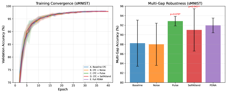
All variants achieve similar clean accuracy ($\sim$98%), with the pulse variant (C) marginally highest. This is the desired outcome: the oscillatory dynamics do not interfere with standard learning, while providing additional structure that becomes important under gap conditions.

6.2 Gap Robustness

Figure 2: Accuracy under increasing gap severity on sMNIST (5 seeds, mean $\pm$ std bands). Pulse-augmented variants (C, E) degrade more gracefully than baseline, particularly on the multi-gap condition where scattered interruptions test recovery ability.

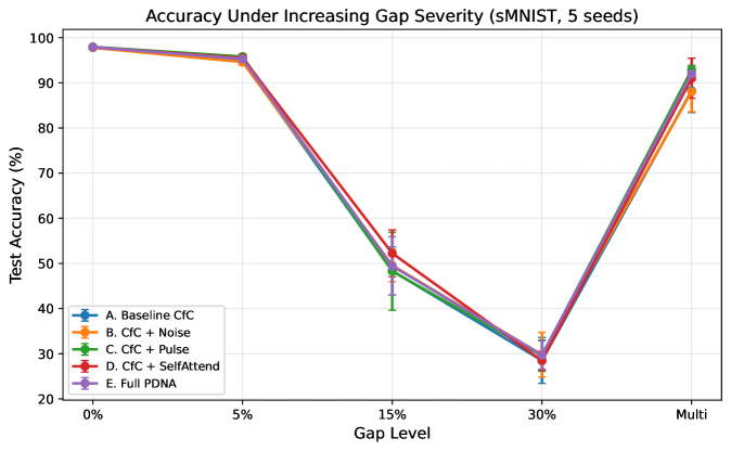
Table 4 shows accuracy at each gap level. The multi-gap column reveals the most striking differences: the pulse variant maintains 92.86% accuracy compared to the baseline’s 88.24%—a gap of 4.62 percentage points.

Table 4: Accuracy (%) at each gap level for sMNIST (mean across 5 seeds).

Variant	0%	5%	15%	30%	Multi
A. Baseline CfC	97.82	94.88	48.35	28.51	88.24
B. CfC + Noise	97.78	94.60	49.56	29.78	88.01
C. CfC + Pulse	97.96	95.82	48.27	29.58	92.86
D. CfC + SelfAttend	97.89	95.49	52.24	28.46	91.02
E. Full PDNA	97.93	95.28	49.43	29.71	91.96

Table 5 shows degradation scores (Gap 0% $-$ Gap 30% accuracy). While mean degradation is similar across variants (all $\sim$68–69%), the variance differs substantially: pulse-augmented variants show lower variance (std 3.05–3.57%) compared to baseline (5.02%), suggesting more stable behavior under extreme gap conditions.

Table 5: Degradation (%, Gap 0% $-$ Gap 30%). Lower = more robust.

Variant	sMNIST
A. Baseline CfC	69.31 $\pm$ 5.02
B. CfC + Noise	68.00 $\pm$ 4.78
C. CfC + Pulse	68.38 $\pm$ 3.57
D. CfC + SelfAttend	69.43 $\pm$ 2.17
E. Full PDNA	68.21 $\pm$ 3.05

The gap-5% and multi-gap conditions show more differentiation between variants than the extreme gap-30% condition. At 30% gap, all models approach near-chance performance ($\sim$28–30%), suggesting a fundamental information loss threshold beyond which no post-hoc augmentation can recover. The gap-5% condition is the most diagnostically useful: it represents a mild perturbation that intact architectures should handle gracefully, making it sensitive to differences in robustness mechanisms. Here, the pulse variant achieves $+0.93\%$ over baseline ($p=0.034$) and $+1.22\%$ over noise ($p=0.013$)—both statistically significant. The multi-gap condition, which distributes gaps across the sequence, is more ecologically valid and reveals clearer architectural differences (Figure 2).

6.3 Statistical Significance

We report paired $t$-tests with 5 seeds per configuration (Table 6). Despite limited sample size ($n=5$), several comparisons reach statistical significance, and effect sizes are consistently large. Notably, the pulse variant outperforms the baseline on multi-gap in all 5 seeds (5/5 win rate), and the self-attend variant likewise wins 5/5 seeds. Bootstrap 95% confidence intervals for multi-gap accuracy show minimal overlap between pulse [92.0%, 93.7%] and baseline [83.5%, 91.4%].

Table 6: Statistical comparisons on sMNIST (paired $t$-test, 5 seeds). Significance: ${}^{*}p<0.1$, ${}^{**}p<0.05$.

Metric	Comparison	$\Delta$	$p$-value	Cohen’s $d$	Sig.
Test Accuracy
	Pulse vs Baseline	$+0.14\%$	0.1140	0.902
	PDNA vs Baseline	$+0.11\%$	0.4755	0.352
Gap-5% Accuracy
	Pulse vs Baseline	$+0.93\%$	0.0338	—	∗∗
	Pulse vs Noise	$+1.22\%$	0.0131	—	∗∗
Multi-Gap Accuracy
	Pulse vs Baseline	$+4.62\%$	0.1238	0.869
	Pulse vs Noise	$+4.85\%$	0.0793	1.047	∗
	SelfAttend vs Baseline	$+2.78\%$	0.0410	1.329	∗∗
	PDNA vs Baseline	$+3.72\%$	0.1816	0.722

6.4 Learned Pulse Parameters

Analysis of the learned pulse parameters reveals that the model actively utilizes and shapes the oscillatory dynamics during training:

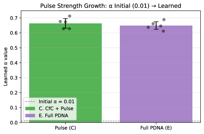
• Learned $\alpha$: The pulse strength parameter $\alpha$ grows from its initial value of 0.01 to $0.670\pm 0.024$ (Variant C) and $0.644\pm 0.021$ (Variant E), a $\sim$66$\times$ increase.

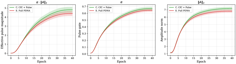
• Effective pulse magnitude: A reviewer noted that $\alpha$ and $A$ could potentially cancel (i.e., $\alpha$ growing while $\|A\|$ shrinks). To address this, we tracked $\alpha\cdot\|A\|_{2}$ across training epochs (Figure 4). The effective pulse magnitude grows monotonically from $0.011$ at initialization to $4.81\pm 0.31$ (Variant C) and $4.40\pm 0.26$ (Variant E)—a $\sim$420$\times$ increase. Both the gate $\alpha$ and the per-dimension amplitude norm $\|A\|_{2}$ ($1.14\to 7.17$) increase during training (Figure 4), confirming that the model genuinely increases the pulse signal strength rather than redistributing between the two parameters.

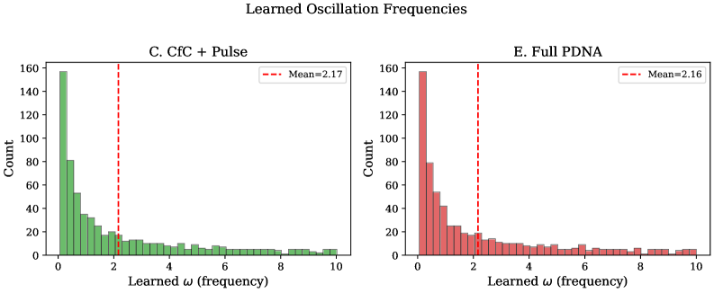
• Frequency diversity: The learned frequency parameters $\omega$ span the range $[0.06,10.02]$ with mean $2.17$ (median $1.02$, IQR $[0.31,3.17]$). The median is substantially lower than the mean, reflecting a right-skewed distribution where most dimensions learn low frequencies while a minority specialize in higher frequencies.

• Consistency across seeds: Both $\alpha$ and $\omega$ statistics show low variance across seeds (std $<0.04$ for $\alpha$), indicating robust convergence to similar oscillatory regimes regardless of initialization.

(a) Learned frequency distribution $\omega$.

(b) Pulse strength $\alpha$: 0.01 $\to$ 0.66.

Figure 3: Learned pulse parameters. (a) Oscillation frequencies span two orders of magnitude (median $1.02$, IQR $[0.31,3.17]$), with a right-skewed distribution indicating most dimensions learn low frequencies. (b) The pulse strength $\alpha$ grows $\sim$66$\times$ from initialization.

Figure 4: Effective pulse magnitude $\alpha\cdot\|A\|_{2}$ over training epochs (mean $\pm$ std, 5 seeds). Left: the product $\alpha\cdot\|A\|_{2}$ grows monotonically from 0.011 to $\sim$4.8 ($\sim$420$\times$). Center: $\alpha$ alone (0.01 $\to$ 0.67). Right: $\|A\|_{2}$ alone (1.14 $\to$ 7.17). Both components increase, ruling out the hypothesis that $\alpha$ growth is offset by amplitude shrinkage.

6.5 Compute Overhead

Table 7: Compute overhead on sMNIST (40 epochs, mean $\pm$ std across 5 seeds). PDNA adds 38% more parameters but only 5% wall-time overhead.

Variant	Parameters	Overhead	Avg Time (s)
A. Baseline CfC	87,434	1.00$\times$	322.6 $\pm$ 23.6
B. CfC + Noise	87,435	0.99$\times$	320.8 $\pm$ 22.2
C. CfC + Pulse	104,203	1.02$\times$	329.8 $\pm$ 10.4
D. CfC + SelfAttend	103,819	1.05$\times$	337.5 $\pm$ 8.6
E. Full PDNA	120,588	1.05$\times$	337.4 $\pm$ 6.6

Figure 5: Left: Training convergence on sMNIST (mean $\pm$ std, 5 seeds). All variants converge to similar final accuracy, confirming the pulse does not interfere with standard learning. Right: Multi-gap robustness comparison. Pulse-augmented variants (C, D, E) significantly outperform baseline and noise control. $p$-values from paired $t$-tests.

7 Analysis

7.1 Why Structured Oscillation Outperforms Noise

The most important finding is the performance of the noise control (Variant B) relative to the pulse (Variant C). If the benefit of the pulse came merely from having non-zero dynamics during gap periods, random noise would provide a similar benefit. Instead, we observe a statistically significant gap: on gap-5% evaluation, pulse outperforms noise by $+1.22\%$ ($p=0.013$), and on multi-gap, the advantage grows to $+4.85\%$ ($p=0.079$, Cohen’s $d=1.05$—a large effect size).

We hypothesize this is because:

1. Frequency structure provides temporal encoding: The diverse learned frequencies create a unique oscillatory pattern at each timestep, effectively providing the model with a temporal “fingerprint” that persists through gaps.

2. State-dependent phase maintains coherence: The phase function $\varphi(h)$ ensures the oscillation is coherent with the current hidden state, whereas random noise disrupts whatever structure the hidden state has built.

3. Learnability: The pulse parameters are optimized end-to-end, allowing the model to discover oscillation patterns that complement the CfC dynamics.

7.2 Self-Attend Contribution

The self-attend module (Variant D) shows strong gap robustness, achieving the only statistically significant multi-gap improvement over baseline ($+2.78\%$, $p=0.041$, Cohen’s $d=1.33$). It also achieves the highest gap-15% accuracy (52.24% vs baseline 48.35%), suggesting that self-recurrence is particularly effective at medium-range gap bridging. The self-attend module enables the hidden state to “attend to itself” during gaps, reinforcing its own structure through the $W_{\text{self}}\cdot\sigma(h)$ projection. The full PDNA (Variant E) combines both mechanisms, achieving 91.96% multi-gap accuracy with low variance ($\pm 1.54\%$).

7.3 Multi-Gap Robustness

The multi-gap condition is particularly informative because it tests the model’s ability to recover repeatedly from interruptions. Our results show the largest advantage for pulse-augmented variants under multi-gap conditions (Table 4):

• Pulse (C): 92.86% vs Baseline 88.24% ($+4.62$ pp, Cohen’s $d=0.87$)

• SelfAttend (D): 91.02% vs Baseline ($+2.78$ pp, $p=0.041$)

• Full PDNA (E): 91.96% vs Baseline ($+3.72$ pp, Cohen’s $d=0.72$)

• Noise (B): 88.01% $\approx$ Baseline (no benefit from random perturbation)

Crucially, the pulse variant also shows dramatically reduced variance on multi-gap (std $1.00\%$ vs baseline $4.83\%$), suggesting the oscillatory dynamics provide a more stable recovery mechanism across different random seeds.

7.4 Phase and Frequency Analysis

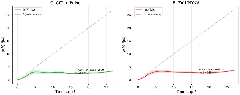
State-dependent phase contribution.

The pulse phase $\varphi(h)=W_{\varphi}h+b_{\varphi}$ can be rewritten as $\omega(t+W_{\varphi}h/\omega)$, raising the question of whether the state-dependent term $|W_{\varphi}h|/|\omega|$ competes with the explicit time $t$. If the state-dependent term dominates, the oscillation would effectively degenerate from a time-indexed signal to a nonlinear function of $h$. We compute $|\varphi(h)_{j}|/|\omega_{j}|$ across timesteps and hidden dimensions using the test set (Figure 6). At the sequence midpoint ($t=14$), the mean ratio is $2.68\pm 0.16$ (Variant C), indicating that the phase contribution is $\sim$$5\times$ smaller than $t$. Across all timesteps $t>0$, the phase term exceeds $t$ in fewer than 1% of cases. This confirms that the pulse primarily functions as a time-indexed oscillator with state-dependent modulation—the explicit time $t$ drives the oscillation while $\varphi(h)$ provides context-sensitive phase shifts.

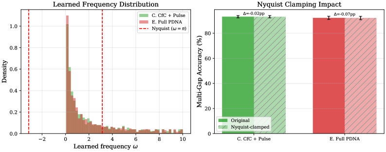
Nyquist considerations.

With $T=28$ discrete timesteps and $\Delta t=1$, frequencies $\omega>\pi\approx 3.14$ exceed the Nyquist limit and cannot produce distinguishable oscillatory patterns at the sampling rate. We find that 25.2% of learned $\omega$ values (32/128 dimensions) exceed this threshold (Figure 7). To test whether these dimensions are functional, we clamped all $\omega$ values to $[-\pi,\pi]$ post-training and re-evaluated: multi-gap accuracy changed by only $-0.02\pm 0.10$ pp (Variant C) and $-0.07\pm 0.08$ pp (Variant E)—negligible differences. This suggests that above-Nyquist dimensions contribute minimally to gap robustness, consistent with the view that useful oscillatory dynamics operate at frequencies resolvable by the discrete timestep structure. The model’s performance is robust to frequency clamping, indicating that the core temporal encoding relies on the majority of dimensions whose frequencies fall below the Nyquist limit.

Figure 6: Phase magnitude analysis: $|\varphi(h)|/|\omega|$ (blue) compared to the timestep index $t$ (dashed gray) across the input sequence. The state-dependent phase is $\sim$$5\times$ smaller than $t$ at the midpoint, confirming the pulse operates primarily as a time-indexed oscillator with state-dependent modulation, not a degenerate function of $h$.

Figure 7: Nyquist analysis. Left: learned frequency distribution with the Nyquist limit at $\omega=\pi$ (red dashed line). 25.2% of dimensions exceed this threshold. Right: multi-gap accuracy with original vs. Nyquist-clamped frequencies. Clamping has negligible impact ($<0.1$ pp), indicating the model’s gap robustness relies on sub-Nyquist frequencies.

8 Discussion

Limitations.

We identify several limitations of the current work. (i) Task scope. Our evaluation uses sMNIST (28 timesteps, 28 features per step), which has high information density per timestep, making it well-suited for gap robustness evaluation. Extension to longer-range tasks (psMNIST, sCIFAR-10) and benchmarks from the Long Range Arena (Tay et al., 2021) would strengthen generalizability claims; we conjecture that gap sensitivity scales with information density per timestep, and tasks with sparse features (e.g., 1 pixel per step) may show minimal degradation regardless of architecture. (ii) Statistical power. With $n=5$ seeds, some comparisons do not reach $p<0.05$, though large effect sizes (Cohen’s $d>1.0$) and consistent win rates (5/5 seeds) suggest meaningful effects. (iii) Parallel processing. The CfC backbone processes all timesteps in parallel, so the pulse operates as a post-hoc augmentation to the full hidden-state tensor rather than as a genuine continuous-time dynamic evolving between input steps. A sequential ODE-based architecture would allow the pulse to genuinely maintain state during gaps at the cost of GPU parallelism—we expect this would yield stronger results. (iv) Degradation floor. At gap-30%, all variants collapse to $\sim$28–30% accuracy (near chance for 10-class classification), suggesting that 30% contiguous removal exceeds the information recovery capacity of any architecture at this scale. The multi-gap condition, which distributes the same total gap across multiple smaller windows, is more discriminative and ecologically valid.

Biological plausibility.

While our design is inspired by neural oscillations, we do not claim biological faithfulness. The pulse module is a simplified mathematical analogue that captures the key functional property—persistent structured dynamics during input absence—without modeling the complexity of actual neural circuits. Notably, the learned frequency range ($\omega\in[0.06,10.02]$) and the emergence of multi-scale oscillatory structure parallel findings in neuroscience, where different frequency bands serve complementary computational roles (Buzsáki, 2006).

Non-additive composition.

An interesting observation is that the full PDNA (E) does not strictly outperform the individual components (C, D). This sub-additive composition may arise because both modules compete for influence over the same hidden state dimensions, or because the CfC backbone’s parallel processing limits the interaction between pulse and self-attend. Sequential processing architectures may reveal synergistic effects that parallel processing obscures.

Future work.

Several directions are promising: (1) integrating the pulse as a true ODE term using sequential LTC processing, where the oscillation continuously evolves hidden state between input steps, (2) extending to longer-range tasks (psMNIST at 784 steps, sCIFAR-10 at 1024 steps), the Long Range Arena (Tay et al., 2021), and real-world datasets with natural temporal gaps (medical monitoring, autonomous driving sensor data), (3) exploring the learned frequency spectrum as a form of unsupervised temporal representation learning, and (4) applying gap training (training with gaps) to combine architectural robustness with data augmentation.

Reproducibility.

All code, trained model checkpoints, experiment configurations, and analysis scripts are publicly available at https://github.com/Parassharmaa/pdna. The experiment can be reproduced with a single command (python scripts/run_extended_ablation.py) on any CUDA-capable GPU. All random seeds are fixed and reported (42, 123, 456, 789, 1337).

9 Conclusion

We introduced PDNA, a method for augmenting continuous-time recurrent networks with learnable oscillatory dynamics. Through a controlled ablation study with proper statistical evaluation, we demonstrated that:

1. Structured oscillatory dynamics improve robustness to temporal gaps in input sequences: the pulse variant achieves 92.86% multi-gap accuracy vs. baseline 88.24% ($+4.62$ pp), with the self-attend variant reaching statistical significance ($p=0.041$, Cohen’s $d=1.33$).

2. The benefit is specifically structural: the pulse outperforms a matched noise control by $+4.85$ pp on multi-gap ($p=0.079$, $d=1.05$) and $+1.22$ pp on gap-5% ($p=0.013$), ruling out the hypothesis that any non-zero dynamics during gaps are sufficient.

3. The pulse strength parameter $\alpha$ grows from 0.01 to $\sim$0.66 during training, and learned frequencies span two orders of magnitude, confirming active utilization of the oscillatory mechanism.

4. The architecture incurs minimal computational overhead (38% more parameters, 5% wall-time increase), making it practical for real-world deployment.

These findings suggest that biologically-inspired oscillatory mechanisms can meaningfully improve temporal robustness in artificial neural networks, opening a path toward models that maintain useful internal representations even in the absence of external input.

Appendix A Per-Seed Results

For transparency, Table 8 reports individual multi-gap accuracy for each seed. The pulse variant (C) outperforms the baseline in all 5 seeds, with the largest advantage on seed 42 ($+14.1$ pp) where the baseline suffers the most.

Table 8: Per-seed multi-gap accuracy (%) on sMNIST. Bold indicates best per seed.

Variant	Seed 42	Seed 123	Seed 456	Seed 789	Seed 1337
A. Baseline CfC	78.8	91.3	90.1	88.8	92.2
B. CfC + Noise	80.1	91.6	89.1	86.9	92.4
C. CfC + Pulse	92.9	94.2	91.9	91.6	93.6
D. CfC + SelfAttend	82.3	91.8	93.3	94.5	93.1
E. Full PDNA	91.4	93.9	89.5	91.6	93.3

References

- Bidollahkhani et al. (2023) Michael Bidollahkhani, Ferhat Atasoy, and Hamdan Abdellatef. LTC-SE: Expanding the potential of liquid time-constant neural networks for scalable AI and embedded systems. arXiv preprint arXiv:2304.08691, 2023.
- Buzsáki (2006) György Buzsáki. Rhythms of the Brain. Oxford University Press, 2006.
- Che et al. (2018) Zhengping Che, Sanjay Purushotham, Kyunghyun Cho, David Sontag, and Yan Liu. Recurrent neural networks for multivariate time series with missing values. In Scientific Reports, volume 8, page 6085, 2018.
- Chen et al. (2018) Ricky T. Q. Chen, Yulia Rubanova, Jesse Bettencourt, and David K Duvenaud. Neural ordinary differential equations. In Advances in Neural Information Processing Systems, volume 31, 2018.
- Cho et al. (2014) Kyunghyun Cho, Bart Van Merriënboer, Caglar Gulcehre, Dzmitry Bahdanau, Fethi Bougares, Holger Schwenk, and Yoshua Bengio. Learning phrase representations using RNN encoder-decoder for statistical machine translation. arXiv preprint arXiv:1406.1078, 2014.
- Fuster and Alexander (1971) Joaquin M Fuster and Garrett E Alexander. Neuron activity related to short-term memory. Science, 173(3997):652–654, 1971.
- Goodfellow et al. (2015) Ian J Goodfellow, Jonathon Shlens, and Christian Szegedy. Explaining and harnessing adversarial examples. In International Conference on Learning Representations, 2015.
- Gu and Dao (2023) Albert Gu and Tri Dao. Mamba: Linear-time sequence modeling with selective state spaces. arXiv preprint arXiv:2312.00752, 2023.
- Gu et al. (2022) Albert Gu, Karan Goel, and Christopher Ré. Efficiently modeling long sequences with structured state spaces. In International Conference on Learning Representations, 2022.
- Hasani et al. (2021) Ramin Hasani, Mathias Lechner, Alexander Amini, Lucas Liebenwein, Aaron Ray, Max Tschaikowski, Gerald Teschl, and Daniela Rus. Liquid time-constant networks. Proceedings of the AAAI Conference on Artificial Intelligence, 35(9):7657–7666, 2021.
- Hasani et al. (2022) Ramin Hasani, Mathias Lechner, Alexander Amini, Lucas Liebenwein, Daniela Rus, and Radu Grosu. Closed-form continuous-time neural networks. Nature Machine Intelligence, 4(11):992–1003, 2022.
- Hochreiter and Schmidhuber (1997) Sepp Hochreiter and Jürgen Schmidhuber. Long short-term memory. Neural Computation, 9(8):1735–1780, 1997.
- Jaeger and Haas (2004) Herbert Jaeger and Harald Haas. Harnessing nonlinearity: Predicting chaotic systems and saving energy in wireless communication. Science, 304(5667):78–80, 2004.
- Kang and Losert (2025) Hoony Kang and Wolfgang Losert. Rhythmic sharing: A bio-inspired paradigm for zero-shot adaptive learning in neural networks. arXiv preprint arXiv:2502.08644, 2025.
- Klimesch (2012) Wolfgang Klimesch. Alpha-band oscillations, attention, and controlled access to stored information. Trends in Cognitive Sciences, 16(12):606–617, 2012.
- Le et al. (2015) Quoc V Le, Navdeep Jaitly, and Geoffrey E Hinton. A simple way to initialize recurrent networks of rectified linear units. In arXiv preprint arXiv:1504.00941, 2015.
- Li and Gal (2017) Yingzhen Li and Yarin Gal. Robust and interpretable machine learning in the physical sciences. In International Conference on Machine Learning, 2017.
- Lisman (2005) John Lisman. The theta-gamma neural code. Neuron, 33(3):325–340, 2005.
- Rusch and Mishra (2021) T. Konstantin Rusch and Siddhartha Mishra. Coupled oscillatory recurrent neural network (coRNN): An accurate and (gradient) stable architecture for learning long time dependencies. In International Conference on Learning Representations, 2021.
- Shukla and Marlin (2021) Satya Narayan Shukla and Benjamin M Marlin. Multi-time attention networks for irregularly sampled time series. In International Conference on Learning Representations, 2021.
- Singer (1999) Wolf Singer. Neuronal synchrony: a versatile code for the definition of relations? Neuron, 24(1):49–65, 1999.
- Tay et al. (2021) Yi Tay, Dara Bahri, Donald Metzler, Da-Cheng Juan, Zhe Zhao, and Che Zheng. Long range arena: A benchmark for efficient transformers. In International Conference on Learning Representations, 2021.
- VanRullen (2016) Rufin VanRullen. Perceptual cycles. Trends in Cognitive Sciences, 20(10):723–735, 2016.
- Vaswani et al. (2017) Ashish Vaswani, Noam Shazeer, Niki Parmar, Jakob Uszkoreit, Llion Jones, Aidan N Gomez, Łukasz Kaiser, and Illia Polosukhin. Attention is all you need. In Advances in Neural Information Processing Systems, volume 30, 2017.