reasonx: Declarative Reasoning on Explanations

Abstract

Explaining opaque Machine Learning (ML) models has become an increasingly important challenge. However, current eXplanation in AI (XAI) methods suffer several shortcomings, including insufficient abstraction, limited user interactivity, and inadequate integration of symbolic knowledge. We propose reasonx, an explanation tool based on expressions (or, queries) in a closed algebra of operators over theories of linear constraints. reasonx provides declarative and interactive explanations for decision trees, which may represent the ML models under analysis or serve as global or local surrogate models for any black-box predictor. Users can express background or common sense knowledge as linear constraints. This allows for reasoning at multiple levels of abstraction, ranging from fully specified examples to under-specified or partially constrained ones. reasonx leverages Mixed-Integer Linear Programming (MILP) to reason over the features of factual and contrastive instances. We present here the architecture of reasonx, which consists of a Python layer, closer to the user, and a Constraint Logic Programming (CLP) layer, which implements a meta-interpreter of the query algebra. The capabilities of reasonx are demonstrated through qualitative examples, and compared to other XAI tools through quantitative experiments.

1 Introduction

The acceptance and trust of Artificial Intelligence (AI) applications is hampered by the opacity and complexity of Machine Learning (ML) models, possibly resulting in biased or even socially discriminatory decision-making (Ntoutsi et al., 2020). As a possible solution, the field of eXplainable Artificial Intelligence (XAI) provides methods to understand how a ML model reaches a decision (Guidotti et al., 2019b; Minh et al., 2022; Mersha et al., 2024). However, most existing approaches focus on descriptive explanations and rarely support declarative reasoning over the decision rationale. By reasoning, we mean the possibility for the user to define any number of conditions over explanations (both factual and contrastive ones), which would codify both background knowledge and what-if analyses (Beckh et al., 2023), and then query for explanations at the symbolic and intensional level. Answers could be expressed in the same language as the user queries, thus making the query language closed, i.e., (part of) the answer to a query can be used in following queries. This would support the interactivity of the explanation process – a requirement of XAI (Miller, 2019).

In this paper, we define a closed algebra of operators on sets of linear constraints. Expressions over such an algebra represent user queries that allow for computing factual and contrastive explanations. On top of the algebra, we design reasonx (reason to explain), an explanation tool that consists of two layers. The first layer is in Python, closer to the data analyst user, where decision trees (DTs) and user queries are parsed and translated. The second layer is in Constraint Logic Programming (CLP) over the reals (Jaffar and Maher, 1994), where embedding of decision trees, and user constraints coding background knowledge are reasoned about. DTs can be themselves the ML models to reason about, or they can be surrogate models of other black-box ML models at the global level or at the local level, i.e., in the neighborhood of an instance to explain. The path from the root to a leaf naturally encodes a linear constraints explaining the decision logic of the DT (or of the black-box model it approximates). Thus, linear constraints over the reals appear a natural knowledge representation mechanism for symbolic reasoning. The expressions of the algebra used at the Python layer are evaluated through a CLP meta-interpreter – a powerful reasoning capability of logic programming (Brogi et al., 1993). The evaluation of expressions produces linear constraints, which are passed back to the Python layer. Since we rely on an intensional symbolic representation of conditions, reasonx offers the unique property of reasoning on under-specified instances, where features may be left unspecified or partly bounded. Moreover, the algebra allows for defining any number of instances and models, hence allowing for reasoning over explanations for the same instance and different models, e.g., models at different points of time.

Figure 1: A simple decision tree illustrating the state of a cup of water in a room at temperature $T_{1}$, which is warmed by a heater contributing an additional temperature $T_{2}$.

Consider a simple example illustrating the need for a high-level abstraction mechanism. Figure 1 shows a simple DT describing the state of a cup of water (“liquid” or “not liquid”), based on room temperature $T_{1}$ and an additional temperature $T_{2}$ contributed by a heater (assuming temperatures are measured in Celsius). Traditional XAI tools typically explain predictions only for fully specified instances. E.g., for $T_{1}=-10,T_{2}=20$, the prediction of the decision tree is “liquid”, and the corresponding factual explanation is the rule $0<T_{1}+T_{2}<100\rightarrow$ “liquid”. At a more abstract (intensional) level, we would be interested in explaining a partially specified instance such as $T_{1}=-10$. In such a case, the prediction “liquid” holds for values of $T_{2}$ such that $10<T_{2}<110$, based on the same factual rule, and the prediction “not liquid” holds for $T_{2}\leq 10$ or $T_{2}\geq 100$. reasonx enables reasoning at precisely this intensional level.

The contributions of this paper are the following:

• We introduce an algebra of operators over sets of linear constraints. The algebra is expressive enough to model complex explanation problems over DTs as expressions (or queries). The algebra is closed, namely the operators can be freely composed.

• We develop the reasonx tool, consisting of two layers. The CLP layer implements an interpreter of the above algebra through meta-programming. The Python layer offers a user-friendly interface specifically designed for ML developers, who can easily integrate models, instances, background knowledge to (silently) generate queries over the algebra and decode back the answers.

• We demonstrate the capabilities of reasonx through qualitative demonstrations, and a quantitative comparison against other XAI tools.

The code of reasonx together with the data used in the demonstrations is publicly available at:

https://github.com/lstate/reasonx

This paper is a substantial extension of two previous works: an introductory paper (State et al., 2023b), targeting an interdisciplinary audience, and a technical paper (State et al., 2023a), providing the preliminary architecture of reasonx. This extension covers the formal definition of the query algebra and its operators, and the definition of explanation problems as queries; an in-depth presentation of the architecture of reasonx, and the demonstrators of its capabilities; as well as the comparison with other XAI tools.

The paper is structured as follows: we discuss the background on XAI topics and related work in Section XAI and Related Work. To keep the paper self-contained, a brief introduction on CLP and meta-reasoning is provided in the Supplemental material. In Section A Query Language over Linear Constraints for XAI, we introduce the algebra of operators, and its capabilities to model explanation problems. The implementation details on reasonx are presented in Section reasonx: Reason to explain. We demonstrate reasonx via some examples in Section Demonstrations, present its evaluation in Section Quantitative Evaluation, and close with limitations and future work in Section Limitations and Future Work. Finally, we close with Section Concluding Remarks. The Supplemental material reports further (experimental) details.

2 XAI and Related Work

XAI aims at coupling effective ML models with explanations of how they work (Guidotti et al., 2019b; Minh et al., 2022; Molnar, 2019; Mersha et al., 2024). This can be achieved through novel explainable-by-design ML models, or through post-hoc explanations of non-interpretable ML models, commonly referred to as black-box models. Post-hoc explanation methods can be categorized with respect to two aspects (Guidotti et al., 2019b). One contrasts model-specific vs. model-agnostic approaches, depending on whether the explanation method exploits knowledge about the internals of the black-box or not. The other aspect contrasts local vs. global approaches, depending on whether an explanation refers to a specific instance or to the black-box as a whole.

In this work, we focus on post-hoc explanations of classification models. Our approach is model-agnostic, as we will reason about a surrogate model of the black-box in the form of a decision tree. The surrogate model can approximate the black-box either globally or locally to a specific instance to explain. In the special case that the black-box is a decision tree itself, i.e., it is too large to be directly understood, our approach is model-specific.

Method (⋆)	Type		Data			Output			CON	DIV	USI	MM	INT
			tab.	text	im.	FR	CR	CE
reasonx	MA/MS	g/l	✓	✗	✗	✓	✓	✓	linear	✓	✓	✓	✓
LORE	MA	l	✓	✗	✗	✓	✓	✗	✗	n.a.	n.a.	✗	✗
GLocalX	MA	g	✓	✗	✗	rule sets		✗	✗	n.a.	n.a.	✗	✗
ANCHORS	MA	l	✓	✓	✓	✓	✗	✗	n.a.	n.a.	n.a.	✗	✗
Wachter	MA	l	✓	✗	✗	✗	✗	✓	✗	✓	✗	✗	✗
DiCE	MA	l	✓	✗	✗	✗	✗	✓	✓	✓	✗	✗	✗
DACE	MS	l	✓	✗	✗	✗	✗	✓	✓	✗	✗	✗	✗
Cui	MS	l	✓	✗	✗	✗	✗	✓	✗	✗	✗	✗	✗
Russell	MS	l	✓	✗	✗	✗	✗	✓	✓	✓	✗	✗	✗
Ustun	MS	l	✓	✗	✗	✗	✗	✓	✓	✗	✗	✗	✗
MACE	MA	l	✓	✗	✗	✗	✗	✓	✓	✓	✗	✗	✗
Karimi	MS	l	✓	✗	✗	✗	✗	✓	✓	✗	✗	✗	✗
Bertossi	MA	l	✓	✗	✗	✗	✗	✓	✓	✗	✗	✗	✗
Takemura	MS	g	✓	✗	✗	rule sets		✗	✓	n.a.	n.a.	✗	✗
LIMEtree	MA	l	✓	✓	✓	✓	✓	✗	✓	n.a.	n.a.	✗	✓

Table 1: Comparing reasonx against related explainability methods. Explanation type according to the introduced taxonomy (MA = model-agnostic, MS = model-specific, g = global, l = local). The output can be factual decision rules (FR), contrastive decision rules (CR) or contrastive examples (CE). CON = possibility to enforce constraints on CR/CE, DIV = possibility of optimizing for diversity on a set of CE. USI = under-specified information for a CE. n.a. = not applicable, tab. = tabular, im. = image. MM = explanations over time and multiple models, INT = interactive explanations.
(^⋆) For space reasons, corresponding papers are listed next: LORE (Guidotti et al., 2019a), GlocalX (Setzu et al., 2021), ANCHORS (Ribeiro et al., 2018), Wachter (Wachter and others, 2017), DiCE (Mothilal et al., 2020), DACE (Kanamori et al., 2020), Cui (Cui et al., 2015), Russell (Russell, 2019), Ustun (Ustun et al., 2019), MACE (Karimi et al., 2020), Karimi (Karimi et al., 2021), Bertossi (Bertossi, 2023), Takemura (Takemura and Inoue, 2024), LIMEtree (Sokol and Flach, 2020a).

Table 1 compares reasonx with related explainability methods. It shows that our tool uniquely combines reasoning over constraints, rules and contrastive examples, over several instances and models, as well as with under-specified instances. We review related work in this section.

2.1 Neuro-symbolic XAI

Calegari et al. (2020) survey how symbolic methods based on some formal logics can be integrated with sub-symbolic models for (neuro-symbolic) explanation purposes. Sabbatini (2025) provides an overview of symbolic knowledge extraction methods from black-boxes. Existing approaches either aim at blending symbolic and sub-symbolic methods (integration), or treat them as distinct parts that remain separated but work together (combination). The central building blocks of these approaches are decision rules, decision trees, and knowledge graphs. Decision rules have been shown to be effective for both developers (Piorkowski et al., 2023) and domain users (Ming et al., 2019; van der Waa et al., 2021).

reasonx relies on a novel usage of constraint logic programming – a form of rule-based symbolic logic reasoning – serving as an explanation tool that adopts the combination approach. Our post-hoc explanation method can be categorized as a “symbolic [neuro]” approach (type 2 in Bhuyan et al. (2024)), where the black-box model is the neuro subroutine called by the symbolic explanation method locally to an instance to explain or globally. The approach is complementary to other neuro-symbolic ones, e.g., “neuro[symbolic]” (type 6) that embeds a symbolic thinking engine directly into a neural engine. Such forms of integration aim at making AI models explainable-by-design.

Other explanation methods exist that borrow concepts from logics but do not allow users to reason over those concepts. The closest ones to our approach are those using (propositional) logic rules as forms of model-agnostic explanations both locally (Ming et al., 2019; Guidotti et al., 2019a; Ribeiro et al., 2018) and globally (Setzu et al., 2021). Another prominent example is TREPAN (Craven and Shavlik, 1995), which computes a decision tree with m-of-n split binary conditions. Further related work in this category is presented by a series of papers by Sokol et al. (Sokol, 2021; Sokol and Flach, 2020a, 2018), based on local surrogate regression trees. Furthermore, Answer Set Programming (ASP), another powerful logic programming extension, has been adopted for local and global explanations of tree ensembles (Takemura and Inoue, 2024), and for contrastive explanations from the angle of actual causality (Bertossi, 2023).

Model-specific logic approaches to XAI offer formal guarantees of rigor, giving rise to the sub-field of formal XAI (Marques-Silva, 2022). In the Supplemental material, we compare sufficient reasons from the formal XAI literature to our notion of factual explanations. Nevertheless, being model-agnostic, our approach does not belong to formal XAI. Recently, epistemic logics have been used to model the justification (i.e., a “proof”) for a belief embedded in an AI model, e.g., for the statements made by Large Language Models (LLMs) (Šekrst, 2025). The justification logic (Artemov and Fitting, 2019), for instance, has been used to provide personalized explanations (Luo et al., 2023) in a multi-agent conversation framework.

2.2 Decision Trees and Factual Explanations

Decision trees (DTs) (Rokach and Maimon, 2005; Costa and Pedreira, 2023) are classification models that predict or describe a nominal feature (the class) on the basis of predictive features, which can be nominal, ordinal or continuous. A decision tree is a tree data structure comprised of internal nodes and leaves. Each internal node points to a number of child nodes, the degree of the node, based on the possible outcomes of a split condition at the node. The split conditions are defined over the predictive features. Here, we will consider binary split conditions in the form of linear inequality constraints. Leaf nodes terminate the tree and are associated with an estimated probability distribution over class labels. The class label with the highest estimated probability is predicted by the DT (Bayes rule) for instances satisfying all split conditions from the root node to the leaf. The highest estimated probability is called the confidence of the prediction.

DTs are inherently transparent and intelligible (Rudin, 2019), unless their size is large. A path from the root note to a leaf corresponds to a conjunction of split conditions that describe the decision rule for class prediction at the leaf. The decision rule of the path followed by an input instance is an explanation for the prediction of the DT over such an instance. This rule-based definition of (factual) explanations is shared with most rule-based explainers (Ming et al., 2019; Guidotti et al., 2019a; Ribeiro et al., 2018; Setzu et al., 2021; Craven and Shavlik, 1995). Sufficient reasons (Izza et al., 2022) (or subset-minimal abductive explanations) from the sub-field of formal XAI consist of a minimal subset of feature values of the instance to explain, such that the prediction of the DT is the same as for the instance regardless of the values of the remaining features. See Amgoud et al. (2023) for a discussion of the relation to the rule-based definition.

A trending research topic in XAI consists of the design of DT learning algorithms that can reproduce the behavior of complex and opaque models, e.g., of a tree ensemble (Weinberg and Last, 2019; Vidal and Schiffer, 2020; Bonsignori et al., 2021; Dudyrev and Kuznetsov, 2021; Ferreira et al., 2022). Such algorithms can be used for training surrogate models, either globally or locally to an instance to explain. Alternative approaches rely on the synthetic generation of a plausible dataset (such as in the neighborhood of the instance to explain) for training surrogate DTs (Guidotti et al., 2019a, 2024; Barbosa et al., 2024). Our research is orthogonal to these topics. We assume a given DT to reason about, independently of whether it is the black-box itself or a global or local surrogate model of a black-box. Nevertheless, high fidelity of a surrogate DT w.r.t. the black-box is a key property that we need to assume in order to support the reasoning over DTs as an approximation of the reasoning over the black-box.

In our approach, we reason over a DT by encoding it as a set of linear constraints. This problem, known as embedding (Bonfietti et al., 2015), requires to satisfy $c(x,y)\Leftrightarrow f(x)=y$, where $f(x)$ is the predicted class by the DT, $x$ is the vector of predictive features, and $c$ is a logic expression. In our approach, $c$ is a disjunction of linear constraints, one for each path from the root to a leaf. This rule-based encoding takes space in $O(n\log{n})$ where $n$ is the number of nodes in the DT. Other DT encodings, such as Table and MDD from Bonfietti et al. (2015), require a discretization of continuous features, thus losing the expressive power of reasoning on linear constraints.

2.3 Contrastive Explanations

Factual explanations, or simply explanations, provide answers to “Why did the input data lead to the provided prediction?”. Contrastive explanations (CEs) refer to data instances similar to the one being explained but with a different predicted outcome. They answer “What should the input data look like, in order to obtain a different output?” which can be easily translated to “How should the current input change to obtain a different output?”, or to answer what-if questions, such as “What happens to the output if the input changes that way?”.

In recent years, contrastive explanations have received considerable attention, as demonstrated by an increasing number of surveys, e.g., (Karimi et al., 2023; Guidotti, 2024; Keane et al., 2021; Stepin et al., 2021). CEs can be represented not only as data instances but also, e.g., as decision rules (Guidotti et al., 2019a), images (Chang et al., 2019) or texts (Wu et al., 2021), and are considered local, model-agnostic explanations. Contrastive explanations have been introduced to XAI by Wachter and others (2017). The authors propose to generate them through the following optimization problem:

$$\arg\min_{x_{ce}}\max_{\lambda}\lambda(f(x_{ce})-y_{ce})^{2}+d(x_{f},x_{ce})$$ (1)

where $f()$ is the ML model, $x_{ce}$ refers to the contrastive instance, $x_{f}$ the original instance, $y_{ce}$ to the prediction to change to, $\lambda$ denotes a tuning parameter, and $d(.,.)$ a distance measure. Intuitively, a CE is the more “realistic” the closer it is to the original instance, understood as the change of as few feature values as possible while $f(x_{ce})$ must align with $y_{ce}$. The optimization function (Equation 1) can be augmented by constraints, e.g., to make the changes actionable (Karimi et al., 2023) or for computing a diverse set of CEs (Mothilal et al., 2020; Laugel et al., 2023). Such an extension can be understood as adding background knowledge to the explanation. Solutions to the optimization problem can be found by reducing it to satisfiability (SAT) or mixed integer linear programming (MILP) problems (Ustun et al., 2019; Russell, 2019; Kanamori et al., 2020). Contrastive explanations (or CXp’s) in the sense of Izza et al. (2022); Audemard et al. (2023) consist of a minimal subset of features of the instance to explain, such that the prediction of the DT is changed for some value of such features, all the other feature values of the instance being unchanged.

reasonx is the first approach adopting CLP for generating CEs. We consider a rule-based definition of CEs, guided by a DT and user-defined constraints linking the instance to explain to its CEs.

2.4 Group Explanations and Under-specified Instances

Local explanations focus on predictions for single instances. Global explanations focus on the decision logic of a black-box for the whole population. Group explanations research considers sub-populations of similar instances with the same predictions, sometimes called cohorts or profiles, that share similar (contrastive) explanations. Existing approaches consist of clustering factual explanations (Setzu et al., 2021) and CEs (Warren et al., 2024). Other works extend the optimization problem of Equation 1 (Carrizosa et al., 2024); focus on explanations that refer to an ensemble of decisions (Artelt et al., 2022); or connect group contrastive explanations to actionable recourse (Rawal and Lakkaraju, 2020).

The literature for local and group explanations deals with an extensional format of instances, i.e., instances are points in a dimensional space, and sub-populations are simply sets of instances. Instead, the symbolic approach of reasonx deals with instances in an intensional format as linear constraints (Cook, 2009). Fully specified instances are defined by setting equality constraints for all features, e.g., age = 20. In addition, under-specified instances can be defined, e.g., bounding the feature values, e.g., age >= 20, or even setting no constraint on that feature. An under-specified instance allows for computing (contrastive) explanations of a specific sub-population. This feature distinguishes our approach.

2.5 Background Knowledge

Exploiting background knowledge in computing an explanation has the potential to significantly improve its quality (Beckh et al., 2023; State, 2021). Background (or prior) knowledge is any information that is relevant in the decision context, but that does not (explicitly) emerge through the data. Not only do simple facts count as such, but we would also consider a natural law as such knowledge, or a specific restriction or requirement a (lay) user has, related to her living reality (e.g., a minimum credit amount in a credit application scenario). Background knowledge integration also draws a connection between our work and the field of actionable recourse (Karimi et al., 2023): this research field proposes explanations not only to explain the model outcome to the affected individual, but also to recommend specific actions so that an undesirable outcome can be changed. Integrated knowledge then helps to better tailor the recommendation to the needs of the user.

reasonx incorporates knowledge in the form of linear constraints over the reals. Some examples of knowledge integration from the literature include: a local explanation tool for medical data that incorporates an ontology to generate a meaningful local neighborhood for explanation generation (Panigutti et al., 2020); a discrimination discovery approach (Ruggieri et al., 2010), where knowledge in the form of association rules is used to detect cases of indirect discrimination; and, in the sub-field of formal XAI, computational complexity investigations of (subset-minimal) abductive and contrastive explanations under domain theories (Audemard et al., 2024) and of constrained classifiers (Cooper and Marques-Silva, 2023).

2.6 Interactivity

Although being acknowledged as a key property of explanation tools (Miller, 2019; Weld and Bansal, 2019; Lakkaraju et al., 2022), few XAI methods incorporate interactivity. Sokol and Flach (2020b) outline the usefulness of interactivity prominently in one of their articles: “Truly interactive explanations allow the user to tweak, tune and personalise them (i.e., their content) via an interaction, hence the explainee is given an opportunity to guide them in a direction that helps to answer selected questions”. We also point to Lakkaraju et al. (2022), presenting an interview study with practitioners and revealing that interactivity for explanations is preferred over static explanations. A notable tool that provides interactive explanations is the glass-box tool (Sokol and Flach, 2018), which can be queried by voice or chat and provides explanations in natural language. Recent advances of LLMs are promising to transform explanations into natural, human-readable narratives (Zytek et al., 2024; Mavrepis et al., 2024).

reasonx natively offers an interactive interface, where explanations can be refined by asserting and retracting constraints, by adding and removing instances and CEs, by projecting to features of interest, and by optimizing tailored distance functions. Since the output of a query to reasonx consists of linear constraints, part of an answer can be readily embedded in subsequent queries by the user. This enables a two-way flow of information, commonly referred to as interaction, between the system and the user.

2.7 Reasoning over Time and Multiple Models

In operational deployment of ML models, it is common that the model changes over time. A change can be induced, for example, by new incoming data that lead to a retraining. Explanation methods that contrast different models are rare. Malandri et al. (2024) present (global) model-contrastive factual explanations of symbolic models, such as decision rules or trees, by computing conditions satisfied by one model and not satisfied by another one. A specific issue is that of contrastive examples that are invalidated by model changes (Barocas et al., 2020). An invalidation can be critical if the CE is intended for the user to seek recourse, i.e., to change the unfavorable model decision by actions proposed by the CE. Ferrario and Loi (2022) call such cases “unfortunate counterfactual events”, and suggest a data augmentation strategy that relies on CE generated previously.

A related case is to compare explanations of the same instance classified by different ML models at the same time. For example, model developers are interested in reasoning on explanations of the same instance with respect to two different but similarly performing models. The instance may have received the same predictions and the same explanations, but different CEs. Or it may have received the same predictions and the same CEs, but different explanations. Pawelczyk et al. (2020) discuss the generation of contrastive explanations for recommendations under predictive multiplicity. This phenomenon refers to different models that give very similar results in performance for a specific prediction problem.

reasonx allows to declare instances and CEs over different models, and to relate them via constraints. This is a natural by-product of the query language reasonx is built on, which is able to cover the case of the same instance and two (or more) different models, either referring to different training times or to different black-box models.

3 A Query Language over Linear Constraints for XAI

We define an algebra of operators over sets of linear constraints. Expressions over the operators define a language of queries. We claim that such a language is expressive enough to model several explanation problems over decision trees as queries.

3.1 Linear Constraints and Decision Trees

A primitive linear constraint is an expression $a_{1}\cdot x_{1}+\ldots a_{n}\cdot x_{n}\simeq b$, where $\simeq$ is in $\{<,\leq,=,\geq,>\}$, $a_{1},\ldots,a_{n}$ are constants in ${\mathbb{R}}$ and $x_{1},\ldots,x_{n}$ are variables. We will use the inner product form by rewriting it as ${\bf a}^{T}{\bf x}\simeq b$, where ${\bf x}=x_{1},\ldots,x_{n}$ is the vector of variables and ${\bf a}=a_{1},\ldots,a_{n}$ the vector of constants. A linear constraint, denoted by $c$, is a sequence of primitive linear constraints, whose interpretation is their conjunction. A path from the root node to a leaf in a decision tree with linear split conditions trivially maps to a linear constraint.

We write $\models\psi$, to denote the validity of the first order formula $\psi$ in the domain of the reals. A constraint $c$ is satisfiable if $\models\exists\ c$, namely if there exists an assignment of all of its variables to real values that evaluates to true in the domain of reals – also called a solution of $c$. The solutions of a linear constraint $c$ are a polyhedron in the space of the variables $\mathbf{x}$. The projection of $c$ over a subset $\mathbf{w}$ of variables is the linear constraint equivalent to existentially quantifying over all variables except $\mathbf{w}$, or in formula $\exists_{-\mathbf{w}}\ c$. The linear projection can be computed by the Fourier-Motzkin projection method (Schrijver, 1987).

We assume any number of decision tree identifiers $DT_{1}$, $DT_{2}$, $\ldots$, each decision tree is defined over the features $\mathbf{x}=x_{1},\ldots,x_{n}$. Also, we assume any number of data instance identifiers (or, simply, instances) $I_{1},I_{2},\ldots$. For each instance $I_{i}$, and feature $x_{j}$, the variable identifier $I_{i}.x_{j}$ is given and called an instance feature. In other words, instance features are variables whose identifiers are prefixed by the instance identifier and suffixed by the feature names. We consider sets of linear constraints over variables including at least the instance features set $\mathcal{F}=\{I_{i}.x_{j}\ |\ i\geq 1,j\in[1,n]\}$.

We call a set of linear constraints a theory. Each constraint in a theory is interpreted as a conjunction of linear inequalities over instance features. The theory as a whole is interpreted as the disjunction of the constraints in the theory.

3.2 An Algebra of Operators

We reason over theories by a closed algebra of operators, i.e., each operator takes theories as input and returns a theory. The syntax of expressions $E$ in the algebra is shown next:

$$E ::= \mathit{inst}(I_{i},DT_{k},l,pr)\ |\ \{U\}\ |\ \mathit{cross}(E+)\ |\ \mathit{sat}(E)\ |\ \pi_{\mathbf{w}}(E)\ |\ \mathit{inf}(E,f(\mathbf{w}))\ |\ \mathit{relax}(E)$$

where $l$ is a constant that denotes a class label, $pr$ is a constant that denotes a probability in $[0,1]$, $\mathbf{w}\subseteq\mathcal{F}$ is a set of instance features, and $f()$ a linear function.

The semantics $Th(E)$ of an expression $E$ is a theory, defined as follows:

• $Th(\mathit{inst}(I_{i},DT_{k},l,pr))$ is the set $\{\wedge_{\mathbf{a}^{T}\mathbf{x}\simeq b\in P}\ \mathbf{a}^{T}I_{i}.\mathbf{x}\simeq b\ |\ P\in DT_{k}(l,pr)\}$ where $DT_{k}(l,pr)$ are the paths in $DT_{k}$ leading to a leaf with class label $l$ predicted with confidence at least $pr$;

• $Th(\{U\})$ is a singleton linear constraint $\{\wedge_{c\in U}c\}$ where $U$ is a sequence of (user-provided) linear constraints;

• $Th(\mathit{cross}(E_{1},\ldots,E_{k}))=\{c_{1}\wedge\ldots\wedge c_{k}\ |\ c_{1}\in Th(E_{1}),\ldots,c_{k}\in Th(E_{k})\}$ is the cross-product of constraints in the theories $Th(E_{1})$, $\ldots$, $Th(E_{k})$;

• $Th(\mathit{sat}(E))=\{c\in Th(E)\ |\ \models\exists\ c\}$ is the set of satisfiable constraints $c$ in $Th(E)$;

• $Th(\pi_{\mathbf{w}}(E))=\{\exists_{-\mathbf{w}}\ c\ |\ c\in Th(E)\}$ is the set of projected constraints $c$ in $Th(E)$;

• $Th(\mathit{relax}(E))=\{c^{=}\ |\ c\in Th(E)\}$ where $c^{=}$ is obtained by replacing strict inequalities in $c$ with inequalities: $<$ is replaced by $\leq$, and $>$ is replaced by $\geq$;

• $Th(\mathit{inf}(E,f(\mathbf{w})))=\{c\wedge(f(\mathbf{w})=(\mathit{inf}{f(\mathbf{w})\ \textrm{s.t.}\,c}))\ |\ c\in Th(E)\}$ is the set of constraints in $Th(E)$ extended with the minimization of $f()$.

Closedness of the algebra is immediate for all operators, with the exception of $\mathit{inf}$. In such a case, if the problem $\inf{f(\mathbf{w})}$ $\textrm{s.t.}\,c$ is unbounded or infeasible, then a linear constraint equivalent to $f(\mathbf{w})=(\inf{f(\mathbf{w})}$ $\textrm{s.t.}\,c)$ is any unsatisfiable one, e.g., $0=1$. If the problem has a solution $v$, then $f(\mathbf{w})=v$ is a linear inequality since $f()$ is linear.

3.3 Explanations as Queries

Factual
Base expression	$e_{1}=\mathit{sat}(\mathit{cross}(\mathit{inst}(I_{1},DT_{1},0,0.95),\{U_{1}\}))$
Factual constraints	$c\in Th(\mathit{inst}(I_{1},DT_{1},0,0.95))$
Factual rule	$c\rightarrow l=0\ [p]$
Constrastive
Base expression	$e_{2}=\mathit{sat}(\mathit{cross}(\mathit{inst}(I_{1},DT_{1},0,0.95),\mathit{inst}(I_{2},DT_{1},1,0.95),\{U_{2}\}))$
Constrastive constraint	$c\in Th(e_{3})$, where $e_{3}=\pi_{I_{2}.\mathbf{x}}(e_{2})$
Contrastive example	any (ground) solution of $c$
Contrastive rule	$c\rightarrow l=1\ [p]$
Minimal contrastive
Base expression	$e_{4}=\mathit{{inf}}(e_{2},f(I_{1}.\mathbf{x},I_{2}.\mathbf{x}))$
Minimal contrastive constraint	$c\in Th(e_{5})$, where $e_{5}=\pi_{I_{2}.\mathbf{x}}(e_{4})$
Minimal contrastive example	any (ground) solution of $c$
Minimal contrastive rule	$c\rightarrow l=1\ [p]$

Table 2: Example expressions for factual, contrastive and minimal contrastive explanations.

We claim that the algebra above is expressive enough to model several explanation problems. We substantiate such a claim with expressions for factual, contrastive, and minimal contrastive explanations. See Table 2 for a summary of example expressions. For ease of presentation, we assume here that the features are continuous. In the next section, we will discuss how reasonx deals with discrete features.

Factual explanations.

Consider the following expression:

$$e_{1}=\mathit{sat}(\mathit{cross}(\mathit{inst}(I_{1},DT_{1},0,0.95),\{U_{1}\}))$$ (2)

where $U_{1}$ is $I_{1}.x_{1}=v_{1},\ldots,I_{1}.x_{n}=v_{n}$, i.e., it fixes the values of the features of the instance $I_{1}$ to constants $v_{1},\ldots,v_{n}$. Then $c\in Th(e_{1})$ iff $c$ consists of the constraints appearing in a path of $DT_{1}$ predicting the class label $0$ with confidence $p\geq 0.95$, and such that the constraints in the path are consistent with the values $v_{i}$’s for the features $x_{i}$’s. In other words, $e_{1}$ tests for a factual explanation for the instance $I_{1}.\mathbf{x}=\mathbf{v}$, where $\mathbf{v}=v_{1},\ldots,v_{n}$. If $Th(e_{1})$ is not empty, such a factual explanation exists. In such a case, the sub-expression $\mathit{inst}(I_{1},DT_{1},0,0.95)$ states why $DT_{1}$ classifies $I_{1}$ with label $l=0$ and confidence $p\geq 0.95$. We call a constraint $c\in Th(\mathit{inst}(I_{1},DT_{1},0,0.95))$ that contributes to $Th(e_{1})$ a factual constraint, and the rule $c\rightarrow l=0\ [p]$ a factual (explanation) rule.

Example.

Consider a decision tree $DT_{1}$ with a single split condition, $x_{1}+x_{2}<5$ that perfectly separates two classes. Instances that match this condition belong to class $l=0$ with confidence $1.0$, while instances that do not match this condition belong to class $l=1$ with confidence $1.0$. We set $U_{1}$ to $I_{1}.x_{1}=2,I_{1}.x_{2}=2$, and we obtain from the tree $Th(inst(I_{1},DT_{1},0,0.95))=\{I_{1}.x_{1}+I_{1}.x_{2}<5\}$. The expression $e_{1}$ evaluates to:

$$Th(e_{1})=\{I_{1}.x_{1}+I_{1}.x_{2}<5\wedge I_{1}.x_{1}=2\wedge I_{1}.x_{2}=2\}=\{I_{1}.x_{1}=2\wedge I_{1}.x_{2}=2\}$$

which is non-empty. The factual rule $I_{1}.x_{1}+I_{1}.x_{2}<5\rightarrow l=0\ [1.0]$ then describes why $DT_{1}$ classifies the instance $I_{1}$ with label $0$ and confidence $1.0$.

Contrastive explanations.

Consider the following expression:

$$e_{2}=\mathit{sat}(\mathit{cross}(\mathit{inst}(I_{1},DT_{1},0,0.95),\mathit{inst}(I_{2},DT_{1},1,0.95),\{U_{2}\}))$$

where $U_{2}$ extends $U_{1}$ by further constraints relating the features of $I_{1}$ and $I_{2}$. Here, it is assumed that the instance $I_{2}$ is classified by $DT_{1}$ with class label $1$, hence it is a contrastive instance w.r.t. $I_{1}$. Then $Th(e_{2})$ is the set of satisfiable constraints specifying: for $I_{1}$ a path in $DT_{1}$ leading to class label $0$ (factual constraints for $I_{1}$); for $I_{2}$ a path in $DT_{1}$ leading to class label $1$ (factual constraints for $I_{2}$); the satisfiability of the constraints between $I_{1}$ and $I_{2}$ stated in $U_{2}$. By projecting over $I_{2}.\mathbf{x}$, that is:

$$e_{3}=\pi_{I_{2}.\mathbf{x}}(e_{2})$$

we obtain constraints over the variables of the contrastive instance $I_{2}$. We call a constraint $c\in Th(e_{3})$ a contrastive constraint, and any solution of $c$ a contrastive example. Intuitively, contrastive examples are the extensional counterpart of the intensional contrastive constraints. Moreover, we call the rule $c\rightarrow l=1\ [p]$, where $p$ is the confidence for $I_{2}$, a contrastive (explanation) rule. Notice that this refers to $I_{2}$ contrasted to $I_{1}$. One can still apply the definition of factual explanation for $I_{2}$, resulting in the factual constraints in $Th(\mathit{inst}(I_{2},DT_{1},1,0.95))$. Notice that more than one instance per class label can be defined. In general, an instance is contrastive w.r.t. any other instance with a different class label. This extends the 1-to-1 settings of one factual and one contrastive rule/example to a $m$-of-$n$ setting of $m$ factual and $n$ contrastive rules/examples. E.g., one can look for a contrastive instance common to two given instances. Such a $m$-of-$n$ setting in XAI is novel.

Example.

We revisit the previous example and keep the same decision tree $DT_{1}$ and the same instance $I_{1}$. Additionally, we define the instance $I_{2}$ such that $Th(inst(I_{2},DT_{1},1,0.95))=\{I_{2}.x_{1}+I_{2}.x_{2}\geq 5\}$. Moreover, $U_{2}$ is defined as $U_{1}$ plus $I_{2}.x_{1}=I_{1}.x_{1}$, namely we add immutability to feature $x_{1}$. Then, the previously introduced expressions evaluate to the following:

$$Th(e_{2}) = \{I_{2}.x_{1}+I_{2}.x_{2}\geq 5\wedge I_{1}.x_{1}=2\wedge I_{1}.x_{2}=2\wedge I_{2}.x_{1}=I_{1}.x_{1}\}$$

$$Th(e_{3}) = \{I_{2}.x_{1}=2\wedge I_{2}.x_{2}\geq 3\}$$

The contrastive rule $I_{2}.x_{1}=2\wedge I_{2}.x_{2}\geq 3\rightarrow l=1\ [1.0]$ describes then a condition under which $DT_{1}$ would classify the instance $I_{2}$ with label $1$ (and confidence $1.0$) and for which the immutability constraint holds. Notice that $I_{2}.x_{1}+I_{2}.x_{2}\geq 5\rightarrow l=1\ [1.0]$ is a factual rule for the instance $I_{2}$.

Minimal contrastive explanations.

Consider the following expression:

$$e_{4}=\mathit{inf}(e_{2},f(I_{1}.\mathbf{x},I_{2}.\mathbf{x}))$$

where $f()$ is a linear (or linearizable) distance function between the instances $I_{1}$ and $I_{2}$. Then $Th(e_{4})$ includes the constraints that, in addition to $Th(e_{2})$, minimize the distance between $I_{1}$ and the contrastive instance $I_{2}$. Given:

$$e_{5}=\pi_{I_{2}.\mathbf{x}}(e_{4})$$

we call a constraint $c\in Th(e_{5})$ a minimal contrastive constraint, and the rule $c\rightarrow l=1\ [p]$, where $p$ is the confidence for $I_{2}$, a minimal contrastive (explanation) rule.

Example

We refer to the previous example, and keep the same decision tree $DT_{1}$, instances $I_{1}$ and $I_{2}$ and constraints $U_{2}$. Further, we define $f(I_{1}.\mathbf{x},I_{2}.\mathbf{x})=\sum_{i}|I_{2}.x_{i}-I_{1}.x_{i}|$, i.e., we use the $L_{1}$ norm as the distance function. The minimal value of $f(I_{1}.\mathbf{x},I_{2}.\mathbf{x})$ occurs when $f(I_{1}.\mathbf{x},I_{2}.\mathbf{x})=|I_{2}.x_{2}-2|+|2-2|=I_{2}.x_{2}-2=1$. The expressions $e_{4}$ and $e_{5}$ evaluate to:

$$Th(e_{4}) = \{I_{1}.x_{1}=2\wedge I_{1}.x_{2}=2\wedge I_{2}.x_{1}=2\wedge I_{2}.x_{2}=3\}$$

$$Th(e_{5}) = \{I_{2}.x_{1}=2\wedge I_{2}.x_{2}=3\}$$

Hence, $I_{2}.x_{1}=2\wedge I_{2}.x_{2}=3\rightarrow l=1\ [1.0]$ is a minimal contrastive explanation.

Explanations for underspecified instances.

Reconsider the previous examples under the revised assumption that $U_{1}$ consists of $I_{1}.x_{1}=2$ only, i.e., we want to reason not on a fully specified instance, but on a set of instances (those for which $x_{1}=2$). It turns out that:

$$Th(e_{1})=\{I_{1}.x_{1}=2\wedge I_{1}.x_{2}<3\}$$

and $Th(e_{3})$ is unchanged. Hence, the contrastive rule holds also in such a case. This means that it is contrastive for all the instances satisfying the constraints stated for $I_{1}$. Regarding the minimal contrastive rule, now $|I_{2}.x_{2}-I_{1}.x_{2}|=I_{2}.x_{2}-I_{1}.x_{2}>0$ since $I_{1}.x_{2}<3$ (see $Th(e_{1})$) and $I_{2}.x_{2}\geq 3$ (see $Th(e_{3})$). The $\mathit{inf}$ operator then imposes $I_{2}.x_{2}=I_{1}.x_{2}$. This leads to an unsatisfiable theory, as it includes both $I_{2}.x_{2}=I_{1}.x_{2}$, $I_{1}.x_{2}<3$, and $I_{2}.x_{2}\geq 3$. The issue is that the minimum of $I_{2}.x_{2}-I_{1}.x_{2}$, under the constraint that it is greater than $0$, does not exist. In practice, $\mathit{inf}$ implements an infimum, but its solution is no longer consistent with the other constraints. We could stop here, accepting no answer to the query. Considering the uncertainty behind decision node splits, we propose instead to relax strict inequalities to inequalities:

$$e^{\prime}_{4}=\mathit{inf}(\mathit{relax}(e_{2}),f(I_{1}.\mathbf{x},I_{2}.\mathbf{x}))\quad\quad\quad e^{\prime}_{5}=\pi_{I_{2}.\mathbf{x}}(e^{\prime}_{4})$$

We then have:

$$Th(e^{\prime}_{4}) = \{I_{1}.x_{1}=2\wedge I_{1}.x_{2}=3\wedge I_{2}.x_{1}=2\wedge I_{2}.x_{2}=3\}$$

$$Th(e^{\prime}_{5}) = \{I_{2}.x_{1}=2\wedge I_{2}.x_{2}=3\}$$

The minimal contrastive constraint $e^{\prime}_{5}=e_{5}$ is unchanged, but the constraint $e^{\prime}_{4}$ differs from the previous one $e_{4}$. The theory of $e^{\prime}_{4}$ contains and therefore constraints both instances $I_{1}$ and $I_{2}$ in such a way as to minimize their distance. Since $I_{1}$ is now underspecified, i.e., a set of instances, this means the minimization will look for the subset of such instances for which the distance is minimal. In this example, such a subset turns out to be a singleton.

On the $\mathit{relax}$ operator.

The need to relax strict inequalities occurs in general only in the case of expressions using the $\mathit{inf}$ operator, since it is actually implemented as an infimum. By applying the $\mathit{relax}$ operator, we basically admit that instances at the boundary of a split condition in a decision tree can be directed to both branches. This is a reasonable assumption, since the boundary of a split condition is the region with the highest predictive uncertainty. As a further extension, reasonx offers a parameter $\epsilon$ to relax strict inequalities with a margin of uncertainty $\epsilon$, e.g., $\mathbf{a}^{T}\mathbf{x}<b$ is relaxed to $\mathbf{a}^{T}\mathbf{x}\leq b+\epsilon$. Again, such a relaxation is reasonable for small $\epsilon$’s, especially when there is aleatoric uncertainty close to the boundary (see Hüllermeier and Waegeman (2021)). In summary, the usage of $\mathit{relax}$ allows to compute additional minimal contrastive explanation (w.r.t. not using it) to account for uncertainty in model decision boundaries.

Explanations over different models: contrastive explanations.

We consider contrastive explanations of a same instance over two different decision trees. These trees can represent either: two models built on different training sets (e.g., trained at different points of time); or, two different models trained on the same training set at the same point of time. The expressions:

$$e_{6}=\mathit{sat}(\mathit{cross}(\mathit{inst}(I_{1},DT_{1},0,0.95),\mathit{inst}(I_{1},DT_{2},0,0.95),$$

$$\hskip 56.9055pt\mathit{inst}(I_{2},DT_{1},1,0.95),\mathit{inst}(I_{2},DT_{2},1,0.95),\{U_{3}\}))$$

$$e_{7}=\pi_{I_{2}.\mathbf{x}}(e_{6})$$

look for conditions for which $I_{1}$ is an instance with the same class label in $DT_{1}$ and $DT_{2}$, and $I_{2}$ is a contrastive instance for both $DT_{1}$ and $DT_{2}$. Such conditions regard contrastive explanations that remain unchanged between $DT_{1}$ and $DT_{2}$.

Example

Let us consider $DT_{1}$ fixed as in the previous examples, and $DT_{2}$ be defined with a single split condition $x_{1}+x_{2}<6$. All instances matching this condition belong to class $l=0$. Let $U_{3}$ include $I_{1}.x_{1}=2,I_{1}.x_{2}=2$ plus $I_{2}.x_{1}=I_{1}.x_{1}$. The expressions $e_{6}$ and $e_{7}$ evaluate to:

$$Th(e_{6}) = \{I_{2}.x_{1}+I_{2}.x_{2}\geq 6\wedge I_{1}.x_{1}=2\wedge I_{1}.x_{2}=2\wedge I_{2}.x_{1}=I_{1}.x_{1}\}$$

$$Th(e_{7}) = \{I_{2}.x_{1}=2\wedge I_{2}.x_{2}\geq 4\}$$

Comparing $Th(e_{7})$ to $Th(e_{3})$, we notice that the minimal contrastive examples for $I_{1}$ that are also minimal contrastive examples for $DT_{2}$ are those for which $I_{2}.x_{1}=2\wedge I_{2}.x_{2}\geq 4$. The ones that are not anymore contrastive in $DT_{2}$ are those for which $I_{2}.x_{1}=2\wedge 4>I_{2}.x_{2}\wedge I_{2}.x_{2}\geq 3$.

4 reasonx: Reason to explain

reasonx is a tool for reasoning over explanations and is based on the query language over constraints introduced in the previous section. Here, we present the architecture of reasonx, the translation of user inputs into queries and of answer constraints into explanations, and the execution of the above queries through a CLP($\mathbb{R})$ meta-interpreter.

Figure 2: Workflow of data, models and explanations for reasonx. To be read from left to right. The three paths show the cases (DT-M), (DT-GS) and (DT-LS) for the base model: base model is a DT model, or a global, or a local surrogate. The explanations are created from the answer constraints produced by a meta-interpreter of the query language over queries generated from user inputs (background and distance), and embeddings of the base model (path constraints).

4.1 reasonx architecture

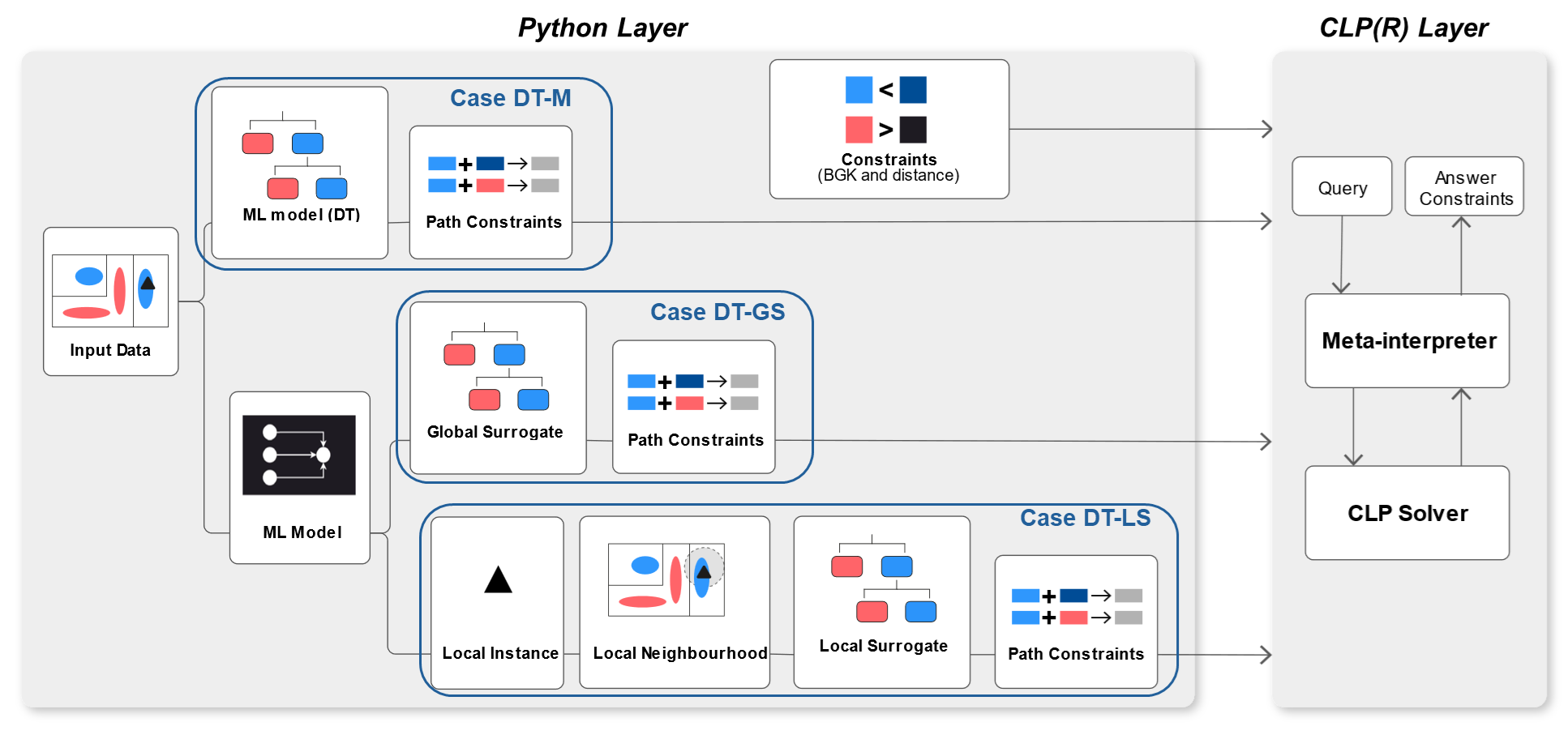
Figure 2 shows the workflow from data, models, and user constraints to queries, and back from answer constraints to explanations. There are two main layers in reasonx. The core layer is written in CLP($\mathbb{R}$) as provided by the SWI Prolog system (Wielemaker et al., 2012). It implements a meta-interpreter for computing the theory $Th(e)$ of an expression $e$ over the language of queries. On top of it, there is a Python layer, which is constructed such that a user – here, a developer – can easily name instances, link them to decision trees, and state user constraints. The Python layer takes care of the meta-data (name and type of features) and of the ML model. It is designed for an easy integration with the pandas and scikit-learn standard libraries for data storage and ML model construction.

reasonx is strongly guided by a decision tree, called the base model. Such a decision tree can be: (DT-M) the model to be explained and reasoned about; (DT-GS) a global surrogate model of a ML model, such as a neural network or an ensemble; or (DT-LS) a local surrogate model trained to mimic a ML model in the neighborhood instances of the instance to explain. Decision trees are directly interpretable only if their size/depth is limited. Large decision trees are hard to reason about, especially in a contrastive explanation scenario. Case (DT-M) can be used in such contexts. In cases (DT-GS) and (DT-LS), the surrogate model is assumed to have high fidelity in reproducing the decisions of the original ML model. This is reasonable for local models, i.e., in case (DT-LS), since learning an interpretable model over a neighborhood has been a common strategy in perturbation-based explainability methods such as LIME (Ribeiro et al., 2016) and LORE (Guidotti et al., 2019a). Explanations produced by reasonx are global in cases (DT-M) and (DT-GS), local in case (DT-LS), model-specific in case (DT-M), and model-agnostic in cases (DT-GS) and (DT-LS).

4.2 Python Layer and Query Generation

Consider the Python layer. Data is stored in tabular form as pandas data frames. One or more decision trees are obtained by one of the cases (DT-M), (DT-GS), and (DT-LS) discussed above. The user can define one or more instances, with the expected class label, and associate each instance to a specific decision tree. Moreover, the user can directly state linear constraints over the features of one or more instances. In addition, the user can fully or partially specify the value of some of the features of an instance. The Python layer transforms decision trees, user constraints, and additional (called, implicit) constraints into CLP($\mathbb{R}$) facts through an embedding procedure described later. The implicit constraints are used to encode the nominal features, which are not directly accounted for in the query language, in a way that is transparent to the user. Then, the Python layer submits one or more expressions over the query language to the CLP($\mathbb{R}$) layer, parses back the answer constraints, and returns, or simply displays, the results to the user.

Let $I_{1},\ldots,I_{m}$ be the instances declared, and $DT_{1},\ldots,DT_{m}$ the linked decision trees. Moreover, let $\Phi$ be the user constraints and $\Psi$ the implicit constraints. The following query expressions are general versions of the ones presented in Section Explanations as Queries:

• $S=\mathit{sat}(\mathit{cross}(inst(I_{1},DT_{1},l_{1},pr_{1}),\ldots,inst(I_{m},DT_{m},l_{m},pr_{m}),\{\Phi,\Psi\}))$ tests satisfiability of the constraints generated from decision trees, stated by the users, and imposed by the data types;

• $F_{i}=inst(I_{i},DT_{i},l_{i},pr_{i})$ is used to generate factual rules of the form $c\rightarrow l=l_{i}\ [p]$ from a path in $DT_{i}$ such that the confidence $p$ of the prediction at the path is such that $p\geq pr_{i}$. The factual rules are produced only for $c$’s that appear as $c\wedge c^{\prime}\in Th(S)$ for some $c^{\prime}$. This condition states that a constraint $c$ from a path of a decision tree must be consistent with the other constraints of the query $S$;

• $CE_{i}=\pi_{I_{i}.\mathbf{x}}(S)$ generates contrastive constraints $c\in Th(CE_{i})$, and contrastive rules of the form $c\rightarrow l=l_{i}\ [p]$. Here, contrastive refers to the other instances $I_{j}$ with the class label $l_{j}\neq l_{i}$. Also, $p$ is the confidence of the prediction of $DT_{i}$ for the path that contributes to $c$;

• $M=\mathit{inf}(\mathit{relax}(S),f(I_{h}.\mathbf{x},I_{k}.\mathbf{x}))$ and $\mathit{MCE}_{i}=\pi_{I_{i}.\mathbf{x}}(M)$ generalize $S$ and $CE_{i}$ to the case of minimal solutions. In particular, minimal contrastive rules are of the form $c\rightarrow l=l_{i}\ [p]$, where $c\in Th(\mathit{MCE}_{i})$ is a minimal contrastive constraint;

• $P=\pi_{\mathbf{w}}(M)$ or $P=\pi_{\mathbf{w}}(S)$ are the most general expressions generated, including the projection of the answer constraints over a set of features $\mathbf{w}\subseteq\mathcal{F}$ required by the user.

The Python layer submits one of the two queries $P=\pi_{\mathbf{w}}(M)$ or $P=\pi_{\mathbf{w}}(S)$ to the CLP($\mathbb{R}$) layer, depending on whether the user requires minimization or not. If the user does not require projection, then $\mathbf{w}=\mathcal{F}$ and $P$ boils down to $M$ or to $S$ respectively. The result of the submitted query, and of the factual rules from $F_{i}$ are returned by the CLP($\mathbb{R}$) layer. For efficiency reasons, the actual implementation does not submit separate queries for the $F_{i}$’s and $CE_{i}$’s, but keeps track of factual and contrastive rules while executing the submitted query. Finally, the user can obtain a contrastive rule $CE_{i}$ by querying $P=\pi_{\mathbf{w}}(S)$ with $\mathbf{w}=I_{i}.\mathbf{x}$.

4.3 From Python to CLP: Embeddings

Let us discuss here how base models, instances, implicit and user constraints are mapped from Python to CLP($\mathbb{R}$) terms and facts.

First, we point out that reasonx is agnostic about the learning algorithm used to produce the base models. We make the following assumptions. Predictive features can be nominal, ordinal, or continuous. Ordinal features are coded as consecutive integer values. Nominal features can be one-hot encoded or not. If not, we force one-hot encoding before submitting the queries to CLP($\mathbb{R}$), and silently decode back from the answer constraints to nominal features before returning the results to the user. In particular, a nominal feature $x_{i}$ is one-hot encoded into features $x_{i}^{v_{1}},\ldots,x_{i}^{v_{k}}$ with $v_{1},\ldots,v_{k}$ being the distinct values in the domain of $x_{i}$. It is important to emphasize that the choice of encoding methods for ordinal and nominal features is non-trivial, as it can significantly impact the performance and fairness of machine learning models (Mougan et al., 2023), as well as the quality of the explanations generated.

We assume that binary split conditions from a parent node to a child node in a decision tree are of the form $\mathbf{a}^{T}\mathbf{x}\simeq b$, where $\mathbf{x}$ is the vector of all features $x_{i}$’s. The following common split conditions are covered by such an assumption:

• axis-parallel splits based on a single continuous or ordinal feature, i.e., $x_{i}\leq b$ or $x_{i}>b$;

• linear splits over features,i.e., ${\bf a}^{T}{\bf x}\leq b$ or ${\bf a}^{T}{\bf x}>b$;

• (in)equality splits for nominal features, i.e., $x_{i}=v$ or $x_{i}\neq v$; in terms of one-hot encoding, they respectively translate into $x_{i}^{v}=1$ or $x_{i}^{v}=0$.

Axis parallel and equality splits are used in CART (Breiman et al., 1984) and C4.5 (Quinlan, 1993). Linear splits are used in oblique (Murthy et al., 1994; Lee and Jaakkola, 2020) and optimal decision trees (Bertsimas and Dunn, 2017). Linear model trees combine axis parallel splits at nodes and linear splits at leaves (Frank et al., 1998).

Base models.

The base models are encoded into a set of Prolog facts, one for each path in the decision tree from the root node to a leaf node:

path($d$,[$\mathbf{x}$], [$\mathbf{a}_{1}^{T}\mathbf{x}\simeq b_{1}$, $\ldots$, $\mathbf{a}_{k}^{T}\mathbf{x}\simeq b_{k}$], $l$, $p$).

where $d$ is an id of the decision tree, [$\mathbf{x}$] is a list of CLP($\mathbb{R}$) variables, one for each feature, $l$ the class predicted at the leaf, $p$ the confidence of the prediction, and [$\mathbf{a}_{1}^{T}\mathbf{x}\simeq b_{1}$, $\ldots$, $\mathbf{a}_{k}^{T}\mathbf{x}\simeq b_{k}$] is the list of the split conditions from the root to the leaf.

Instances.

Each declared instance is encoded by a list of CLP($\mathbb{R}$) variables, one for each feature. The mapping between the feature name and the variable is positional. All the instances are collectively represented by a list of lists of variables.

Implicit constraints ($\Psi$).

A number of constraints on the features $\mathbf{x}$ of each instance naturally derive from the data type of the features. We call them implicit constraints, because the system can generate them from meta-data about features:

• for continuous features: $x_{i}\in{\mathbb{R}}$;

• for ordinal features: $x_{i}\in\mathbb{Z}$ and $m_{i}\leq x_{i}\leq M_{i}$ where $dom(x_{i})=\ \{m_{i},\ldots,M_{i}\}$ is the domain of $x_{i}$;

• for one-hot encoded nominal features: $x^{v_{1}}_{i},\ldots,x^{v_{k}}_{i}\in\mathbb{Z}$ and $\wedge_{j=1}^{k}(0\leq x^{v_{j}}_{i}\leq 1)$ and $\sum_{j=1}^{k}x^{v_{j}}_{i}=1$;

We denote by $\Psi$ the conjunction of all implicit constraints.

User constraints ($\Phi$).

A number of user constraints or background knowledge, loosely categorized as in Karimi et al. (2023), and extended based on work by Karimi et al. (2021); Ustun et al. (2019); Mothilal et al. (2020); Mahajan et al. (2019) can be readily expressed in reasonx. We provide examples and use $F$ to refer to a factual instance and $CE$ to refer to a corresponding contrastive instance. Feasibility constraints concern the possibility of feature changes between the factual and contrastive instance, and how changes depend on previous values or other features. A feature that is unconstrained in feasibility is actionable without any condition. Among the feasibility constraints, we can distinguish:

• Immutable features: a feature cannot or must not change between the factual and contrastive instances, e.g., the birthplace: $CE.{\mathit{birthplace}}=F.{\mathit{birthplace}}$.

• Mutable but not actionable features: the change of a feature from the factual to the contrastive instance is only a result of changes in the features it depends upon. An example is the change of unit scale, e.g., from Euro to US Dollars, which can be encoded as $CE.{\text{€}}=1.16\cdot CE.{\mathdollar}$ – assuming a conversion rate of $1.16$.

• Actionable but constrained features: a feature can be changed only under some conditions, e.g., age can only increase : $CE.{\mathit{age}}\geq F.{\mathit{age}}$.

Another class regards consistency constraints, which aim at bounding the domain values of a feature, e.g., $0\leq CE.{\mathit{age}}\leq 120$ limits the age feature in the range $[0,120]$.

Encoding distance functions.

The assumption that instances have a specific predicted class label (see operator $\mathit{inst}$), allows us to remove the first term from Equation 1, hence reducing the problem of computing minimal contrastive explanations to minimize the distance function between the factual and contrastive instances. reasonx offers two distance functions that can be used with the $\mathit{inf}$ operator: $L_{1}$ combined with a matching norm for the nominal variables (referred to as as $L_{1}$ norm for the remainder of this paper) and $L_{\infty}$, both over normalized features. The $L_{1}$ norm penalizes the average change over all features, while the $L_{\infty}$ norm penalizes the maximum changes over all features. See also Wachter and others (2017); Karimi et al. (2020) for a discussion of how the different norms affect the generated contrastive explanations. In the Supplemental material, we show how to linearize such norms, i.e., how to express them using linear constraints only, possibly introducing slack variables and adding further implicit constraints to $\Psi$.

Regarding the diversity of the contrastive explanations, we combine the approach of Lampridis et al. (2023) and the diversity evaluation of Mothilal et al. (2020). Assume that we have a (factual) instance $I_{f}$ and a large pool of contrastive instances. From this pool, our objective is to select a diverse subset of $|S|$ instances. reasonx encodes the following distance:

$$f(x_{f},S)=\frac{\lambda}{|S|}\sum_{i\in S}dist(I_{f}.\mathbf{x},I_{i}.\mathbf{x})-\frac{1}{|S|^{2}}\sum_{i\in S}\sum_{j\in S}dist(I_{i}.\mathbf{x},I_{j}.\mathbf{x})$$ (3)

where $S$ is a set of indices of contrastive instances w.r.t. $I_{f}$, and $\lambda$ is a tuning parameter. The first term measures the distance between the factual and the contrastive instances (proximity), the second term the distance within the set of contrastive instances (diversity). Thus, minimization of the function optimizes the trade-off between proximity and diversity.

4.4 CLP Layer and the Meta-interpreter

The core engine of reasonx is a CLP($\mathbb{R})$ meta-interpreter of expressions over the query language presented in Section A Query Language over Linear Constraints for XAI.

Meta-reasoning is a powerful technique that allows a logic program to manipulate programs encoded as terms. In CLP, meta-reasoning is extended by encoding also constraints as terms (Wielemaker et al., 2012). For example, consider Listing 1.

⬇

1satisfiable(P) :-

2 copy_term(P, CopyP),

3 tell_cs(CopyP).

4tell_cs([]).

5tell_cs([C|Cs]) :-

6 {C},

7 tell_cs(Cs).

Listing 1: Definition of predicates satisfiable and tell_cs.

The query tell_cs([X >= 0, Y = 1 - X]) asserts the linear constraints in the list, adding them to the constraint store. Linear constraints can be the result of some manipulation beforehand. For example, the query satisfiable([X = 0, Y >= 1 - X]) first makes a copy of the list by renaming all variables into fresh ones, and then it asserts the copy to the constraint store. In this way, the assertion succeeds if and only if the constraints are satisfiable, but without altering the original constraints, e.g., without fixing X to $0$.

Here, we discuss a simplified version of the reasonx interpreter using the predicate solve($E$, $Vars$, $C$), where $E$ is the expression to interpret, $Vars$ is the list of lists of variables (one list per instance), and $C$ is the returned answer constraint consisting of $Th(E)$. We proceed with the interpretation of each operator.

($\{U\}$)

The interpretation of the $\{U\}$ operator is split into two base operators: userc for the user constraints and typec for the implicit constraints that cover the data types. Listing 2 shows that the former simply retrieves the list of constraints $\Psi$ embedded in the user_constraints predicate by the Python layer. The latter appends the lists of constraints for nominal variables and ordinal variables. Details on the called predicates are omitted.

⬇

1solve(userc, Vars, Cons) :-

2 user_constraints(Vars, Cons).

3

4solve(typec, Vars, Cons) :-

5 cat_constraints(Vars, CCat),

6 ord_constraints(Vars, COrd),

7 append(CCat, COrd, Cons).

Listing 2: Interpretation of the $\{U\}$ operator.

($\mathit{inst}$)

The operator $\mathit{inst}(I,DT,l,pr)$ is interpreted in Listing 3. The position $N$ of $I$ in the list of all instances is decoded through the data_instance predicate asserted by the Python layer. The interpreter accesses the variables $V$ of $I$ (predicate nth0), and matches them with the embedding of a path in the $DT$ decision tree that ends in a leaf with class label $l$ and with predicted accuracy $P$. Finally, only paths for which $P$ is at least the required probability $pr$ are considered.

⬇

1solve(inst(I, DT, L, Pr), Vars, Cons) :-

2 data_instance(N, I),

3 nth0(N, Vars, V),

4 path(DT, V, Cons, L, P),

5 P >= Pr.

Listing 3: Interpretation of the $\mathit{inst}$ operator.

($\mathit{cross}$)

The interpretation of the $\mathit{cross}(L)$ operator is stated by recursively solving the tail list of $L$ and the head of $L$, and then calculating the cross-product of the constraints in the returned results.

⬇

1solve(cross([]), _, []).

2solve(cross([T|Ts]), Vars, Cons) :-

3 solve(cross(Ts), Vars, TsCons),

4 solve(T, Vars, TCons),

5 append(TCons, TsCons, Cons).

($\mathit{sat}$)

The $\mathit{sat}(T)$ operator is interpreted as shown in Listing 4. After solving the sub-expression $T$, the resulting constraints are checked for satisfiability through the satisfiable predicate. Such a predicate takes also as input the list of variables in the domain of the integers. By using the meta-programming capabilities of CLP($\mathbb{R}$), after making a fresh copy of its inputs through the built-in predicate copy_term, the satisiability is checked by: (1) asserting the copy of the constraints using tell_cs (see Listing 1); and (2) checking that among the solutions there is one assigning integer values to integer variables using the bb_inf predicate. In this last call, the argument 0 regards the (constant) function to minimize, and the unnamed variable “_” concerns the returned minimum value (not used).

⬇

1solve(sat(T), Vars, Cons :-

2 solve(T, Vars, Cons),

3 int_vars(Vars, IntVars),

4 satisfiable(Cons, IntVars).

5

6satisfiable(Cons, Ints) :-

7 copy_term(Cons-Ints, CopyCons-CopyInts),

8 tell_cs(CopyCons),

9 bb_inf(CopyInts, 0, _).

Listing 4: Interpretation of the $\mathit{sat}$ operator.

($\pi$)

The interpretation of the $\pi_{\mathbf{w}}(T)$ operator is provided in Listing LABEL:lst:project. After solving $T$, the projection of the solution over the features $\mathbf{w}$ is implemented by the meta-predicate project designed by Benoy et al. (2005).

⬇

1solve(project(T, PVars), Vars, PCons) :-

2 solve(T, Vars, Cons),

3 project(PVars, Cons, PCons).

($\mathit{inf}$)

Finally, let us consider inf(T, F) in Listing 5. After solving $T$ into constraints $\mathit{TCons}$, the interpreter linearizes the expression $F$ regarding the distance function into a linear expression $\mathit{LinF}$, possibly generating additional constraints $\mathit{ConF}$. Satisfiability of the union of $\mathit{TCons}$ and $\mathit{ConF}$ is checked with an extended version of satisfiable. Such a variant also computes the infinum value of $\mathit{LinF}$ taking into account the integer variables $\mathit{IntVars}$. The infinum value $\mathit{Min}$ is returned by satisfiable together with integer assignments for the integer variables. Such assignments are turned into equality constraints, and together with the key equality $\mathit{LinF}=\mathit{Min}$ from the definition of the $\mathit{min}$ operator (see Section An Algebra of Operators) appended to the other constraints.

⬇

1solve(inf(T, F), Vars, Cons) :-

2 solve(T, Vars, TCons),

3 exp_eval(F, Vars, LinF, ConF),

4 append(ConF, Cons, ConsMin),

5 int_vars(Vars, IntVars),

6 satisfiable(ConsMin, IntVars, LinF, Min, IntValues),

7 eq_con(IntVars, IntValues, ConsEq),

8 append([LinF=Min|ConF], Cons, Cons1),

9 append(CEq, Cons1, Cons).

Listing 5: Interpretation of the $\mathit{min}$ operator.

Integer-linear constraints.

The variant of satisfiable used in the interpretation of $\mathit{inf}$ is based on the MILP built-in predicate bb_inf($C$, $\mathit{IntVars}$, $\mathit{LinF}$, $\mathit{Min}$, $\mathit{IntValues}$). The extension to MILP problems is required because (one-hot encoded) nominal and ordinal features lie in the domain of the integers. We discuss here the implications of such an extension on the query language of Section A Query Language over Linear Constraints for XAI.

For the given integer variables $\mathit{IntVars}$, a call to the bb_inf predicate returns only one answer, i.e., without backtracking (for efficiency reasons, since there may be an exponential number of solutions), with ground values $\mathit{IntValues}$. Such values have the property that the linear function $\mathit{LinF}$ reaches its minimum over $C$ at the minimum of $C\wedge(\mathit{IntVars}=\mathit{IntValues})$. The latter turns out to be a linear constraint. Instead, the minimization of $C$ in presence of integer variables is an NP-hard problem that cannot always be expressed as a linear constraint (Karp, 1972). The implication for reasonx is that, when integer variables are present (namely, in presence of ordinal or nominal features), the returned answer constraint is a correct but not complete characterization of the space of solutions to the query. For instance, consider the query:

$$\mathit{min}(\{0\leq x\leq 1,0\leq y\leq 1,x-y\leq z,y-x\leq z\},z)$$

with the assumption that $x,y\in\mathbb{Z}$. This query is intended to constrain $z$ to $|x-y|$, the absolute value of the difference between $x$ and $y$. Such constraints naturally arise in the modeling of $L_{1}$ and $L_{\infty}$ distances. The variables $x$ and $y$ are set to the ground values returned by bb_inf, namely $x=0,y=0$, and the minimum is reached for $z=0$. Hence, the interpreter returns $x=0,y=0,z=0$. This is a correct answer constraint, but it does not cover all possible solutions. For example, $x=1,y=1,z=1$ is another solution which is never explored.

5 Demonstrations

Here, we present several use-cases to illustrate the functionalities of reasonx. The majority of these demonstrations is based on case (DT-M), i.e., under the assumption that the base model is also the ML model. For an overview of the corresponding experimental settings, see Table 11 in the Supplemental material, which also reports additional examples.

5.1 Synthetic Dataset

We define a small synthetic dataset, consisting of two features (feature1 and feature2) and a binary class with values 0 and 1, each class having $1,000$ data instances. These are sampled from different bivariate normal distributions that are almost separable by an axis-parallel decision tree. We choose a data instance from class 0, called the factual instance (“factual” in the figures), to illustrate some of the functionalities of reasonx at the Python layer. To initialize reasonx, the following code is needed.

⬇

1USER: r = reasonx.ReasonX(pred_atts, target, df_code)

2 r.model(clf1)

The constructor takes as input the list of features and the class name, and an object (df_code) that decodes categorical features. The base DT clf1 is set via the model method.

As a first operation, we set a factual instance of interest, named F, using the method instance, and query reasonx through the solveopt method.

⬇

1USER: r.instance(’F’, features=[1100, 661], label=0)

2 r.solveopt()

F is fully specified as all feature values are set. The query generated and solved by the CLP layer is of the form $e_{1}$ as in (2). There is a single contraint in $Th(e_{1})$. The output of reasonx shows such a constraint (called answer constraint) and the respective factual rule $c\rightarrow l=0$ with confidence $1.0$.

⬇

1REASONX: Answer constraint:

2 F.feature1=1100.0,F.feature2=661.0

3 Rule satisfied by F:

4 IF F.feature2> -55.5,F.feature1>1004.0 THEN class 0 [1.0]

To help intuition, we also plot the results. The left-hand side $c$ of the factual rule is shown as factual region in Figure 3 (left).

Figure 3: Left: factual region (FR) as provided by reasonx. Right: contrastive regions (CR) as provided by reasonx. Grey lines refer to the decision boundary of the base DT.

Next, we ask for the contrastive constraints, i.e., feasible regions of contrastive instances. We code the problem by declaring an additional instance with the name CE, with class label 1, and now requiring a minimum confidence of $0.8$ for its factual rule (or contrastive rule in relation to the first instance).

⬇

1USER: r.instance(’CE’, label=1, minconf=0.8)

2 r.solveopt()

⬇

1REASONX: Answer constraint:

2 F.feature1=1100.0,F.feature2=661.0,CE.feature2<= -55.5,CE.feature1<=1043.5

3 Rule satisfied by F:

4 IF F.feature2> -55.5,F.feature1>1004.0 THEN class 0 [1.0]

5 Rule satisfied by CE:

6 IF CE.feature2<= -55.5,CE.feature1<=1043.5 THEN class 1 [0.9974]

7--

8 Answer constraint:

9 F.feature1=1100.0,F.feature2=661.0,CE.feature2> -55.5,CE.feature1>466.0,

10 CE.feature1<=1004.0

11 Rule satisfied by F:

12 IF F.feature2> -55.5,F.feature1>1004.0 THEN class 0 [1.0]

13 Rule satisfied by CE:

14 IF CE.feature2> -55.5,CE.feature1>466.0,CE.feature1<=1004.0

15 THEN class 1 [0.9939]

Figure 3 (right) shows the two contrastive regions denoted by the left-hand sides of the two rules for CE.

Notice that the instances F and CE are not related, apart from being predicted by the DT with different classes. This means that while we interpret instance CE as contrastive to instance F, it could be also interpreted as a different factual instance. We then use a constraint to ensure that feature2 stays constant between the factual instance and the contrastive one (see Figure 4 (left)), or to ensure that instead feature1 stays constant (Figure 4 (right)). While the first constraint leads to an admissible contrastive region as a line (CE.feature2 = 661.0, CE.feature1 > 466.0, CE.feature1 <= 1004.0), the second constraint leads to no solution.

Figure 4: Left: contrastive region (CR) as provided by reasonx, and given a constraint on feature2. Right: given the constraint on feature1, no solution exists. The dashed line refers to the enforced constraint. Grey lines refer to the decision boundary of the DT.

The following code shows these cases. Before the second constraint is asserted, the first constraint needs to be retracted (see second USER code box, line 1). Retraction facilitates interactivity: asserted constrains accumulate one after the other, until they are retracted.

⬇

1USER: r.constraint(’CE.feature2 = F.feature2’)

2 r.solveopt()

⬇

1REASONX: Answer constraint:

2 F.feature1=1100.0,F.feature2=661.0,CE.feature2=661.0,CE.feature1>466.0,

3 CE.feature1<=1004.0

4 Rule satisfied by F:

5 IF F.feature2> -55.5,F.feature1>1004.0 THEN class 0 [1.0]

6 Rule satisfied by CE:

7 IF CE.feature2> -55.5,CE.feature1>466.0,CE.feature1<=1004.0

8 THEN class 1 [0.9939]

⬇

1USER: r.retract(’CE.feature2 = F.feature2’)

2 r.constraint(’CE.feature1 = F.feature1’)

3 r.solveopt()

⬇

1REASONX: No answer.

Now, we extend the example by asking for the closest contrastive points lying over the identity line (CE.feature2 = CE.feature1). The minimization of the $L_{1}$ norm between F and CE is passed as an argument to solveopt. From now on, we omit the output of the rules (this can be set with the method verbosity()).

⬇

1USER: r.retract(last=True)

2 r.constraint(’CE.feature2 = CE.feature1’)

3 r.solveopt(minimize=’l1norm(F, CE)’, project=[’CE’])

⬇

1REASONX: Answer constraint:

2 F.feature1=1100.0,F.feature2=661.0,CE.feature1= -55.5,CE.feature2= -55.5

3 Min value: 0.894

4--

5 Answer constraint:

6 F.feature1=1100.0,F.feature2=661.0,CE.feature1=1004.0,CE.feature2=1004.0

7 Min value: 0.185

Figure 5 (left) reports the two solutions returned by reasonx – shown as red dots. Both of them stay in the identity line. They are the closest instances for each of the contrastive regions characterized by leaves of the DT. In fact, reasonx solves the optimization problem for each of those independently and provides the user therefore not with the global optimum, but with two local optima. This leaves more flexibility to the user. Further processing of the results, e.g., filtering for the global optimum, can be implemented. The data point CE.feature1 = 1004.0, CE.feature2 = 1004.0 denoted by CE 2 in Figure 5 (left) is the global optimum. The distance between such pairs is the one reported in the output of reasonx.

Let us now allow feature2 of the factual instance to be under-specified, by setting it to a range instead of a fixed value. We reset all constraints, and assert the value for feature1 and bounds for feature2. In the solveopt we also add another parameter to project the answer constraint over the CE instance only. Figure 5 (right) shows the region of the two answer constraints: a single point and a line. Each point in the line represent a closest point to some of the possible values for F.

⬇

1USER: r.reset(keep_model=True)

2 r.instance(’F’, label=0)

3 r.constraint(’F.feature1 = 1100, F.feature2 >= 161,

4 F.feature2 <= 1161’)

5 r.instance(’CE’, label=1, minconf=0.8)

6 r.solveopt(minimize=’l1norm(F, CE)’, project=[’CE’])

⬇

1REASONX: Answer constraint:

2 CE.feature1=1043.5,CE.feature2= -55.5

3 Min value: 0.115

4--

5 Answer constraint:

6 CE.feature1=1003.99999,CE.feature2>=161.0,CE.feature2<=1161.0

7 Min value: 0.051

Figure 5: Left: minimal CEs provided by reasonx, under the constraint denoted by the identity line. Right: minimal CEs provided by reasonx for under-specified instances. Grey lines refer to the decision boundary of the DT.

5.2 Reasoning over Time

Description	Output
$\mathcal{R_{F,\text{$0$}}}$	IF F0.capitalgain<=5095.5, F0.education<=12.5, F0.age>29.5
	THEN <=50K [0.8095]
$\mathcal{R_{F,\text{$1$}}}$	IF F1.capitalgain<=5119.0, F1.education<=12.5, F1.age>33.5
	THEN <=50K [0.7907]

Table 3: Factual rules $\mathcal{R_{F,\text{$i$}}}$ for a same instance and different models over time $DT_{i}$ with $i=0,1$.

reasonx can be run on several models and instances. Here, we assume the following case: a model is used over a long period of time, and it undergoes re-training due to new, incoming data instances. The re-training induces small model changes.

We simulate this case by splitting the Adult Income dataset into two datasets of the same size, and training the same type of model under the same parameter settings on these two splits. Let $DT_{0}$ and $DT_{1}$ be the resulting decision trees.

Independent explanations.

First, we define two instances F0 and F1, assigning the same data values to them, but a different model – $DT_{0}$ and $DT_{1}$ respectively. We independently query for factual and contrastive rules, and for the minimal CEs under the $L_{1}$ norm. Results are displayed in Table 3 for the factual rules and in Table 4 for the contrastive rules and examples. In both cases, three contrastive rules and three minimal contrastive examples are generated. The contrastive examples (4) and (10) are the same.

Index	Output (rules or contrastive examples)
(1)	$\mathcal{R_{C,\text{$0$}}}$	IF CE0.capitalgain<=5095.5,CE0.education>12.5,CE0.age>30.5
		THEN >50K [0.5087]
(2)	$\mathcal{R_{C,\text{$0$}}}$	IF CE0.capitalgain>5095.5,CE0.capitalgain<=6457.5 THEN >50K [0.9286]
(3)	$\mathcal{R_{C,\text{$0$}}}$	IF CE0.capitalgain>7055.5,CE0.age>20.0 THEN >50K [0.9873]
(4)	$CE_{0}$	CE0.race=AsianPacIslander, CE0.sex=Male,CE0.workclass=Private,
	($0.267$)	CE0.education=13.0,CE0.age=40.0,CE0.capitalgain=0.0,
		CE0.capitalloss=0.0,CE0.hoursperweek=40.0
(5)	$CE_{0}$	CE0.race=AsianPacIslander, CE0.sex=Male,CE0.workclass=Private,
	($0.051$)	CE0.education=9.0,CE0.age=40.0,CE0.capitalgain=5095.51,
		CE0.capitalloss=0.0,CE0.hoursperweek=40.0
(6)	$CE_{0}$	CE0.race=AsianPacIslander, CE0.sex=Male,CE0.workclass=Private,
	($0.071$)	CE0.education=9.0,CE0.age=40.0,CE0.capitalgain=7055.51,
		CE0.capitalloss=0.0,CE0.hoursperweek=40.0
(7)	$\mathcal{R_{C,\text{$1$}}}$	IF CE1.capitalgain<=5119.0,CE1.education>12.5,CE1.age>29.5
		THEN >50K [0.5125]
(8)	$\mathcal{R_{C,\text{$1$}}}$	IF CE1.capitalgain>5119.0,CE1.capitalgain<=5316.5 THEN >50K [1.0000]
(9)	$\mathcal{R_{C,\text{$1$}}}$	IF CE1.capitalgain>7073.5,CE1.age>20.5 THEN >50K [0.9904]
(10)	$CE_{1}$	CE1.race=AsianPacIslander,CE1.sex=Male,CE1.workclass=Private,
	($0.267$)	CE1.education=13.0,CE1.age=40.0,CE1.capitalgain=0.0,
		CE1.capitalloss=0.0,CE1.hoursperweek=40.0
(11)	$CE_{1}$	CE1.race=AsianPacIslander,CE1.sex=Male,CE1.workclass=Private,
	($0.051$)	CE1.education=9.0,CE1.age=40.0,CE1.capitalgain=5119.01,
		CE1.capitalloss=0.0,CE1.hoursperweek=40.0
(12)	$CE_{1}$	CE1.race=AsianPacIslander,CE1.sex=Male,CE1.workclass=Private,
	($0.071$)	CE1.education=9.0,CE1.age=40.0,CE1.capitalgain=7073.51,
		CE1.capitalloss=0.0,CE1.hoursperweek=40.0
(13)	$\mathcal{R_{C,\text{$0,1$}}}$	IF CE.capitalgain>5095.5,CE.capitalgain<=5119.0,CE.education>12.5,
		CE.age>29.5 THEN >50K [0.5125]
(14)	$CE_{0,1}$	CE.race=AsianPacIslander,CE.sex=Male,CE.workclass=Private,
	($0.318$)	CE.education=13.0,CE.age=40.0,CE.capitalgain=5095.51,
		CE.capitalloss=0.0,CE.hoursperweek=40.0

Table 4: Contrastive rules and examples for a same instance and different models. Rules $\mathcal{R_{C,\text{$0$}}}$ and examples $CE_{0}$ in (1) - (6) refer to $DT_{0}$. Rules $\mathcal{R_{C,\text{$1$}}}$ and examples $CE_{1}$ in $\mathcal{R_{C,\text{1}}}$ in (7) - (12) refer to $DT_{1}$. Rule $\mathcal{R_{C,\text{$0,1$}}}$ and example $CE_{0,1}$ in (13) and (14) refer to additional conditions that are the result of intersecting explanations from $DT_{0}$ and $DT_{1}$. Numerical values in round brackets indicate the distance between factual instance and contrastive examples.

Intersecting explanations.

Now, we use the reasoning capabilities of reasonx to better understand how these two sets of explanations relate to each other. In order to do so, we use the output produced for instance F0 (the answer constraints) as an additional input before querying for contrastive rules and instances of instance F1. This is achieved using the r.constraint() method to assert the answer constraints. As a result, we obtain four rules that are not only contrastive to $F1$ but also to $F0$ and thus in their intersection. Three out of these four rules can be identified as rule (1), (8) and (9) in Table 4. There is also a novel rule, displayed under index (13). This rule is the intersection of rule (2) and (7). Similarly, we obtain the contrastive examples (4/10), (11) and (12) in Table 4, and a new example (14). With this approach, we obtained the intersection of the previously (independently) derived contrastive rules, meaning that the obtained contrastive rules are valid in both models. Similarly, the computed contrastive examples are valid in both models. If we remind ourselves of the time dimension, it means that the change in the model over time became indeed visible in its explanation and that some of the contrastive rules and instances derived at the first time point (model $DT_{0}$) are no longer valid at the second time point (model $DT_{1}$) as they are not contained in the intersection of both.

5.3 Reasoning over Different Model Types

Description	Output
$\mathcal{R_{F,\text{$0$}}}$	IF F0.capitalgain>7055.5,F0.age>20.0 THEN >50K [0.9882]
$\mathcal{R_{F,\text{$1$}}}$	IF F1.education<=12.5,F1.capitalgain>7073.5 THEN >50K [0.9940]

Table 5: Factual rules $\mathcal{R_{F,\text{$i$}}}$ for a same instance and different models types $DT_{i}$ with $i=0,1$.

Index	Output (rules)
(1)	$\mathcal{R_{C,\text{$0$}}}$	IF CE0.capitalgain<=5119.0,CE0.education<=12.5,CE0.age<=30.5
		THEN <=50K [0.9653]
(2)	$\mathcal{R_{C,\text{$0$}}}$	IF CE0.capitalgain<=5119.0,CE0.education<=12.5,CE0.age>30.5
		THEN <=50K [0.8032]
(3)	$\mathcal{R_{C,\text{$0$}}}$	IF CE0.capitalgain<=5119.0,CE0.education>12.5,CE0.age<=28.5
		THEN <=50K [0.9022]
(4)	$\mathcal{R_{C,\text{$0$}}}$	IF CE0.capitalgain<=5119.0,CE0.education>12.5,CE0.age>28.5
		THEN <=50K [0.5068]
(5)	$\mathcal{R_{C,\text{$0$}}}$	IF CE0.capitalgain>5316.5,CE0.capitalgain<=7055.5
		THEN <=50K [0.7400]
(6)	$\mathcal{R_{C,\text{$0$}}}$	IF CE0.capitalgain>7055.5,CE0.age<=20.0 THEN <=50K [0.8000]
(7)	$\mathcal{R_{C,\text{$1$}}}$	IF CE1.education<=12.5,CE1.capitalgain<=4243.5,
		CE1.capitalloss<=1805.0 THEN <=50K [0.9760]
(8)	$\mathcal{R_{C,\text{$1$}}}$	IF CE1.education>12.5,CE1.sex_Female<=0.5,CE1.age<=29.5
		THEN <=50K [0.9474]
(9)	$\mathcal{R_{C,\text{$1$}}}$	IF CE1.education>12.5,CE1.sex_Female>0.5,
		CE1.capitalgain<=4718.5 THEN <=50K [0.9395]
(10)	$\mathcal{R_{C,\text{$0,1$}}}$	IF CE.capitalgain<=4243.5,CE.education<=12.5,CE.age<=30.5,
		CE.capitalloss<=1805.0 THEN <= 50K [0.9653]
(11)	$\mathcal{R_{C,\text{$0,1$}}}$	IF CE.capitalgain<=5119.0,CE.education>12.5,CE.age<=28.5,
		CE.sex_Female<=0.5 THEN <= 50K [0.9022]
(12)	$\mathcal{R_{C,\text{$0,1$}}}$	IF CE.capitalgain<=4718.5,CE.education>12.5,CE.age<=28.5,
		CE.sex_Female>0.5 THEN <= 50K [0.9022]

Table 6: Contrastive rules for a same instance and different model types. Rules $\mathcal{R_{C,\text{$0$}}}$ in (1) - (6) refer to $DT_{0}$. Rules $\mathcal{R_{C,\text{$1$}}}$ in (7) - (9) refer to $DT_{1}$. Rules $\mathcal{R_{C,\text{$0,1$}}}$ in (10) - (12) refer to additional conditions that are the result of intersecting explanations from $DT_{0}$ and $DT_{1}$.

In this section, we show how reasonx can be used to reason over different model types. As an example, we compare a DT model (case (DT-M)) with a ML model that is explained via a global surrogate model, i.e., case (DT-GS). A simple comparison between a random forest (RF), a multi-layer perceptron (MLP), and an XGBoost (XGB) model shows that the latter slightly outperforms the former models (an accuracy of $0.851$ against $0.814$ for the MLP and $0.808$ for the RF, in comparison $0.802$ for the DT). We therefore compare the DT with the XGB model. The fidelity, i.e., the ratio of correct prediction of the global surrogate DT w.r.t. prediction of the XGB model is $fidelity=0.919$.

Independent explanations.

We compare the factual decision rules behind a the same data instance. The results are depicted in Table 5. The reasons behind the classification of the data instance, i.e., the features appearing on the left-hand side of the rules, are different – even if both models correctly classify the instance as class >50K. Both models use the feature capitalgain, but while the DT (model $0$) relies on the feature age, the XGB model (model $1$) uses the feature education.

We expect to see these differences also in the contrastive decision rules. These are displayed in Table 6. Three aspects immediately stand out. First, the DT offers more contrastive rules than the XGB model. Second, the confidence values of the DT are on average lower than for the XGB ($0.786$ versus $0.954$, on average). Third, the feature sex, a sensitive attribute, appears only in the contrastive rules of the XGB.

Intersecting explanations.

We compute the intersection between the contrastive rules of both models, using the same approach as in Section Reasoning over Time. However, we restrict the rules to those that have a minimum confidence value of $0.9$, i.e., we intersect only rules with the index (1), (3), and (7) - (9) from Table 6. This restriction is a conscious choice and can be easily enforced by declaring the minconf when initializing the contrastive instances using r.instance(...). As a result, we obtain rule (10) as the intersection between (1) and (7), rule (11) as the intersection between (3) and (8), and rule (12) as the intersection between (3) and (9).

Recalling that we compare two different ML models trained on the same dataset and that have a small gap in performance, we observe that these two models, according to reasonx, draw on different reasons for the same classification. Further, only one of the two models makes use of a sensitive attribute. This is an important observation: while model performance matters, it cannot be the only determining reason to choose a specific model for an application. Rather, it is important why a model produced a specific output. Understanding that these reasons can be very different for similarly well performing models trained on the same dataset is thereby an integral part.

In general, more reasoning operations using reasonx are possible, such as reasoning over the produced contrastive explanations (similar to the demonstration in Section Reasoning over Time), or reasoning over more than two ML models.

5.4 Diversity Optimization

In this experiment, we select three contrastive explanations from an admissible set of contrastive explanations, using the optimization function discussed in Section From Python to CLP: Embeddings, paragraph Encoding distance functions.. We run this experiment on the Adult Income dataset, case (DT-M) and for a decision tree with a depth of $depth=5$. This parameter is changed to obtain a higher number of contrastive examples. Furthermore, we set $\lambda=0.5$ and repeat the optimization for $50$ instances.

Results are compared to the classical approach of selecting contrastive instances, i.e., optimizing only by proximity. In both cases, we compute the value of the optimization function $f(x_{f},S)$ and of the proximity and diversity term separately. We plot the results in Figure 6 (see the Supplemental material in Diversity Optimization). The classical approach leads to a distribution of values of the optimization function that has a sharp peak and is centered around zero. When considering the diversity of generated contrastive explanations in the optimization, the distribution of the function changes: values are much more diverse, there is no sharp peak. To confirm that these values indeed belong to different distributions, we calculated the Kolmogorov-Smirnow test ($p$-value $\approx 0$).

5.5 Detecting Biases

Here, we demonstrate how the generation of contrastive examples and the use of constraints in reasonx can support the detection of societal biases. This case is close to the definition of explicit bias as in Goethals et al. (2024) and may be useful in the context of direct discrimination and prima facie discrimination. We investigated a DT and an XGB model, and possible discrimination based on the sensitive attributes age, race, sex, and pairwise combinations.

In summary, we find that in the case of a DT, reasonx does not highlight potential biases. For the XGB model, the influences of age and sex on the predicted outcome may be relevant. Details on the experiment, more information on bias detection through XAI and definitions, as well as details on the experimental results can be found in the Supplemental material in Detecting Biases.

6 Quantitative Evaluation

In this section, we present the quantitative evaluation of reasonx. We start by evaluating reasonx only. Then, we compare (minimal) contrastive examples of reasonx against those produced by DiCE (Mothilal et al., 2020), and factual rules of reasonx against those produced by ANCHORS (Ribeiro et al., 2018). The chosen approaches approximate two aspects of reasonx separately so that a fair comparison is possible on these aspects. In addition, we compare the runtime of the three approaches. Information on experimental details and datasets can be found in Section Experiments in the Supplemental material.

The metrics used in this section are standard metrics (Vilone and Longo, 2021; Pawelczyk et al., 2021; Guidotti et al., 2019a), adapted to the characteristics of reasonx as a tool based on CLP. Details on metrics are discussed in Section Metrics in the Supplemental material.

Also, the Supplemental material contains experiments on the parameters of reasonx in Section Parameter Testing.

6.1 Results

	case	$acc/f$ (⋆)	$l_{F}$	$l_{C}$	$N_{C}$	$S/N$		$N_{CE}$	$d_{CE}$	$dim_{CE}$
ADULT	(DT-M)	$0.802$	$2.988$	$2.008$	$2.049$	$0.82$	$L_{1}$	$2.049$	$0.063$	p.
							$L_{\infty}$	$2.049$	$0.062$	h.-d.
	(DT-GS)	$0.851/0.919$	$2.978$	$2.832$	$4.674$	$0.92$	$L_{1}$	$4.674$	$0.449$	p.
							$L_{\infty}$	$4.674$	$0.378$	h.-d.
	(DT-LS)	$0.851/0.840$	$1.944$	$2.564$	$2.371$	$0.89$	$L_{1}$	$2.371$	$0.244$	p.
							$L_{\infty}$	$2.371$	$0.201$	h.-d.
SGC	(DT-M)	$0.737$	$3.0$	$3.0$	$3.208$	$0.77$	$L_{1}$	$3.208$	$0.762$	p.
							$L_{\infty}$	$2.922$	$0.515$	h.-d.
	(DT-GS)	$0.757/0.767$	$2.986$	$2.739$	$3.217$	$0.767$	$L_{1}$	$3.217$	$0.687$	p.
							$L_{\infty}$	$2.565$	$0.514$	h.-d.
	(DT-LS)	$0.757/0.797$	$2.947$	$2.961$	$3.092$	$0.76$	$L_{1}$	$3.092$	$0.819$	p.
							$L_{\infty}$	$2.632$	$0.515$	h.-d.
GMSC	(DT-M)	$0.936$	$3.0$	$2.0$	$1.0$	$0.95$	$L_{1}$	$1.0$	$0.020$	p.
							$L_{\infty}$	$1.0$	$0.015$	h.-d.
	(DT-GS)	$0.936/0.984$	$2.041$	$2.666$	$3.020$	$0.98$	$L_{1}$	$3.020$	$0.022$	p.
							$L_{\infty}$	$3.020$	$0.019$	h.-d.
	(DT-LS)	$0.936/0.880$	$2.500$	$2.587$	$4.294$	$0.34$	$L_{1}$	$4.235$	$0.266$	p.
							$L_{\infty}$	$4.294$	$0.228$	h.-d.
DCCC	(DT-M)	$0.780$	$3.0$	$3.0$	$1.081$	$0.74$	$L_{1}$	$0.865$	$0.150$	p./h.-d.
							$L_{\infty}$	$1.081$	$0.148$	h.-d.
	(DT-GS)	$0.778/0.926$	$3.0$	$3.0$	$1.064$	$0.94$	$L_{1}$	$0.819$	$0.148$	p./h.-d.
							$L_{\infty}$	$1.064$	$0.145$	p.
	(DT-LS)	$0.778/0.940$	$2.411$	$2.603$	$2.011$	$0.90$	$L_{1}$	$1.533$	$0.495$	p./h.-d.
							$L_{\infty}$	$2.011$	$0.400$	h.-d.
ACA	(DT-M)	$0.845$	$3.0$	$3.0$	$4.506$	$0.83$	$L_{1}$	$4.506$	$0.942$	p.
							$L_{\infty}$	$4.506$	$0.897$	h.-d.
	(DT-GS)	$0.850/0.857$	$2.796$	$2.796$	$3.389$	$0.857$	$L_{1}$	$3.389$	$0.768$	p.
							$L_{\infty}$	$3.389$	$0.705$	h.-d.
	(DT-LS)	$0.850/0.990$	$2.013$	$2.497$	$2.425$	$0.80$	$L_{1}$	$2.25$	$1.037$	p.
							$L_{\infty}$	$2.25$	$0.862$	h.-d.

Table 7: Evaluation of reasonx. SGC = South German Credit, GMSC = Give Me Some Credit, DCCC = Default Credit Card Clients, ACA = Australian Credit Approval. The CE obtained after the MILP optimization can be a point (abbreviated p.) or a higher-dimensional object such as a line (abbreviated h.-d.). (^⋆) No fidelity in case (DT-M).

reasonx only.

Results for reasonx are shown in Table 7. Results depend on the dataset and case. Lengths of factual and contrastive rules are in most cases not the same but of similar size. In most cases, the number of solutions of contrastive rules and constraints (for both norms) is the same, i.e., an example could be identified on all admissible paths of the DT. Also, the values of the $L_{1}$ norm are always a bit larger than values for the $L_{\infty}$ norm. Excluding the DCCC datasets, for the $L_{1}$ norm, only points (zero-dimensional) are obtained while the $L_{\infty}$ norm returns higher-dimensional objects (solutions to linear constraints are polyhedra, in general). This is due to the latter penalizing only the maximum change over all features while the first penalizes all changes.

		$N_{CE}$		$d_{CE}$ ($w_{div}=0$)
Setting/Approach	$acc/f$	$L_{1}$	$L_{inf}$	$L_{1}$	$L_{inf}$
No constraints
DiCE	$0.785$ (*)	2		1.131	0.775
		3		1.097	0.754
		4		1.170	0.784
		5		1.107	0.767
REASONX (case DT-GS)	$0.851/0.919$	$4.674$	$4.674$	$0.449$	$0.378$
REASONX (case DT-LS)	$0.851/0.840$	$2.371$	$2.371$	$0.244$	$0.201$
Immutability on capitalgain
DiCE	$0.785$ (*)	2		1.128	0.778
		3		1.167	0.808
		4		1.125	0.777
		5		1.113	0.778
REASONX (case DT-GS)	$0.851/0.919$	$1.935$	$1.935$	$0.581$	$0.516$
REASONX (case DT-LS)	$0.851/0.840$	$0.011$	$0.011$	$1.467$	$1.0$
Immutability on race and sex
DiCE	$0.785$ (*)	2		0.976	0.680
		3		0.994	0.683
		4		0.983	0.687
		5		0.974	0.668
REASONX (case DT-GS)	$0.851/0.919$	$3.674$	$3.674$	$0.217$	$0.202$
REASONX (case DT-LS)	$0.851/0.840$	$2.371$	$2.371$	$0.244$	$0.201$

Table 8: Contrastive examples/constraints: comparison between DiCE and reasonx. (*) No fidelity for DiCE.

Constrative examples.

A comparison between reasonx and DiCE is provided in Table 8. Distances of reasonx are smaller than those obtained with DiCE, i.e., the contrastive examples are closer to the original data instance. An exception is case (DT-LS) under the immutability constraint on capitalgain. When constraints are enforced, less solutions are found by reasonx. Such a behavior is expected as adding constraints cuts down on the admissible paths in the (constant) base model. The change in the distance between factual and contrastive depends then on the CE that remain on the admissible paths. In DiCE, the number of contrastive examples is a parameter. No general statement can be made about the change in the distance.

Approach	$acc$/$f$	$D$	$p_{0}$ or $MC_{F}$ (⋆⋆)	$p_{c}$	$c$ or $S/N$ (⋆⋆)	$l_{F}$
ANCHORS	$0.850$ (⋆)	n.a.	$0.9$	$0.910$	$0.433$	$2.06$
			$0.95$	$0.944$	$0.352$	$3.04$
			$0.99$	$0.966$	$0.273$	$4.55$
reasonx (case DT-GS)	$0.851/0.891$	2	$0.9$	n.a.	$0.69$	$2.0$
			$0.95$	n.a.	$0.69$	$2.0$
			$0.99$	n.a.	$0$	n.a.
reasonx (case DT-LS)	$0.851/0.839$	2	$0.9$	n.a.	$0.87$	$1.011$
			$0.95$	n.a.	$0.86$	$1.0$
			$0.99$	n.a.	$0.23$	$1.0$
reasonx (case DT-GS)	$0.851/0.919$	3	$0.9$	n.a.	$0.81$	$2.975$
			$0.95$	n.a.	$0.7$	$2.971$
			$0.99$	n.a.	$0.02$	$2.0$
reasonx (case DT-LS)	$0.851/0.840$	3	$0.9$	n.a.	$0.78$	$1.936$
			$0.95$	n.a.	$0.72$	$1.931$
			$0.99$	n.a.	$0.39$	$1.923$
reasonx (case DT-GS)	$0.851/0.929$	4	$0.9$	n.a.	$0.79$	$3.127$
			$0.95$	n.a.	$0.79$	$3.127$
			$0.99$	n.a.	$0.02$	$3.0$
reasonx (case DT-LS)	$0.851/0.846$	4	$0.9$	n.a.	$0.66$	$2.136$
			$0.95$	n.a.	$0.66$	$2.136$
			$0.99$	n.a.	$0.59$	$2.068$

Table 9: Factual rules: comparison between reasonx and ANCHORS. (^⋆) ANCHORS has no fidelity. (^⋆⋆) The first metric ($p_{0}$ or $c$) is reported for ANCHORS, the second ($MC_{F}$ or $S/M$) is a non-equivalent but similar metric for reasonx.

Factual rules.

Results on factual rules produced by reasonx and ANCHORS are displayed in Table 9. For ANCHORS, the higher the precision the lower the coverage of the extracted rule. Also, the rule length increases with precision. In reasonx, the rule length correlates with the depth of the decision tree. For a fixed depth $D$, the higher the minimum confidence $MC_{F}$ the smaller the ratio $S/N$. This is expected as a higher minimum confidence restricts the number of admissible paths in the base model. The average rule length is less than or equal to the tree depth and decreases (slightly) with higher minimum confidence.

Approach	Setting	Constraints	Time (in s)
reasonx	initialization (⋆)	n.a.	$0.129$
	case DT-M, $D=3$, $MC_{F}=0$
	initialization, query	no constraints	$1.102$
	initialization, query	immutability capitalgain	$0.685$
	case DT-GS, $D=3$, $MC_{F}=0$
	initialization, query	no constraints	$0.825$
	initialization, query	immutability capitalgain	$0.574$
	case DT-LS, $D=3$, $MC_{F}=0$
	initialization, query	no constraints	$1.375$
	initialization, query	immutability capitalgain	$0.891$
ANCHORS	$p_{0}=0.9$	n.a.	$0.558$
	$p_{0}=0.95$	n.a.	$0.942$
	$p_{0}=0.99$	n.a.	$0.974$
DiCE	$N_{CE}=2$	no constraints	$0.445$
	$N_{CE}=2$	immutability capitalgain	$0.382$
	$N_{CE}=3$	no constraints	$0.169$
	$N_{CE}=3$	immutability capitalgain	$0.117$
	$N_{CE}=4$	no constraints	$0.212$
	$N_{CE}=4$	immutability capitalgain	$0.158$
	$N_{CE}=5$	no constraints	$0.247$
	$N_{CE}=5$	immutability capitalgain	$0.142$

Table 10: Runtime for reasonx, ANCHORS and DiCE. (^⋆) relies on case (DT-M).

Runtime.

We report runtimes of reasonx, ANCHORS and DiCE Table 10. Runtimes of reasonx are higher compared to the runtimes of ANCHORS and DiCE, excluding high precision values of ANCHORS and case (DT-GS) of reasonx. This is expected, given its higher complexity and expressivity of reasonx and the overhead due to communication between Python and CLP($\mathbb{R})$. For ANCHORS, runtimes increase with an increased precision parameter $p_{0}$. For DiCE, while no systematic change can be observed when the parameter $N_{CE}$ is increased, runtimes decrease if an immutability constraint is added. The same decrease in runtime with an additional constraint can be observed for reasonx. In addition, runtimes for reasonx are highest for case (DT-LS). This is expected as case (DT-LS) is the most complex one: one base model has to be learned per instance.

6.2 Completeness, Coverage, and Constraint Validity

The following statements regarding the completeness, coverage and validity of reasonx hold, assuming that its base model was learned successfully, i.e., that accuracy (case (DT-M)) or fidelity (case (DT-GS) and (DT-LS)) are sufficiently high. This is guaranteeing a certain level of correctness between the base model’s prediction and the original class (case (DT-M)) or the predicted class (case (DT-GS) and (DT-LS)): first, under no additional constraints, for every data instance, reasonx can find the factual, and one or more contrastive rules. It can also find one or more contrastive data instances. If no factual rule is returned, this is because the prediction of the base model does not agree with the data label (case (DT-M)) or the prediction of the approximated ML model (case (DT-GS) and (DT-LS)), or because the parameter of the minimum confidence value is too high. However, this is an intentional design choice and reasonx can still retrieve the results by a change in the query – to explain the incorrect prediction of the base model, or to provide an explanation with a lower confidence value. Additionally, for the returned contrastive rule and the contrastive constraints/examples, an additional check of the prediction w.r.t. the black-box ML model in cases (DT-GS) and (DT-LS) is needed to ensure that they are indeed located on the other side of the decision boundary. Such a check is currently not implemented, relying on the assumption of very high fidelity of the surrogate DT to the black-box model. A possible future implementation consists of relying on a dataset of instances (possibly, a synthetic one) to estimate the precision of the contrastive rule. This is a non-trivial problem when the instance to explain is under-specified. Second, the average length and the number of the obtained (factual or contrastive) rules depend on the depth and the width of the base model (see also Section Quantitative Evaluation), and the distance between the original and the contrastive instances may not be minimal w.r.t. the original decision boundary, as the base model only approximates the boundary. Third, all data instances in the input space of the base model are covered by factual rules which have no overlap – only one rule is the factual rule. Other XAI approaches based on rules do not have this property, therefore (Lakkaraju et al., 2016; Vilone and Longo, 2021) introduce a metric called “fraction overlap”. Fourth, if constraints are enforced in reasonx, the rules – if they exist – align with the constraints. This is not always the case for XAI approaches based on rules, thus, (Pawelczyk et al., 2021) introduce a metric called “constraint violation” specifically for contrastive explanations.

7 Limitations and Future Work

Let us discuss here the limitations and future work of our approach regarding its evaluation, technical aspects, the user-perspective, and social assumptions.

Evaluation.

From the theoretical side, reasonx advances other methods in qualitative terms. However, further work is needed to verify this also from a practical side: how the tool is perceived by expert or lay users, how easy it is to encode and reason about domain knowledge as constraints, and how the approach scales in presence of noise and non-separable classes. This validation can be conducted through user studies (see Rong et al. (2024) for a survey specifically on XAI) and through real-world case studies. Regarding the application setting of this paper, namely the credit domain, some reference literature on credit scoring and ML/XAI and can be found at Bücker et al. (2022); Demajo et al. (2020); Shi et al. (2022). We further re-emphasize that the cases presented in this paper are constructed and do not represent real-world conditions.

Technical.

We demonstrated the capabilities of reasonx on tabular data, and for binary decision problems. While an extension to multi-class problems is straightforward, the extension to unstructured data, such as text and images, needs to be strictly formalized. In the domain of images, a solution can be the integration of concepts, as shown, e.g., by Donadello and Dragoni (2020). Moreover, the extension of the approach to other constraint (logic programming) schemes beyond linear constraints over the reals is a relevant direction, including, for instance, finite domains, non-linear constraints, or probabilistic/fuzzy logic programming. The literature on such extensions is large (Morettin et al., 2021; Körner et al., 2022). To adapt our framework to such extensions, the key requirement is to preserve the closedness property of the extended language, ensuring that the optimization and reasoning capabilities remain sound and tractable. Moreover, it will be worth investigating how domain knowledge expressed in other formalisms (e.g., knowledge graphs) can be encoded and reasoned about as constraints.

User-centered.

We aim at extending reasonx along the perspective of the Human-XAI interaction (Chromik and Butz, 2021). First, by improving the Python layer through the integration of a plotting functionality (to produce similar plots as in Section Synthetic Dataset), and additional syntactic sugar functionalities, e.g., to express a class label of the form “not class X” for the generation of contrastive rules. Second, by adding a natural language layer on top of the Python layer for an easier communication with users (see also next section). Third, by experimenting with the quality of explanations containing constraints (Byrne, 2023), and with the known implications of XAI methods, such as automation bias (Vered et al., 2023).

Social.

Two basic assumptions of reasonx must be taken care of in socially-sensitive applications, where contrastive rules might be used as recommendations to change the decision (a.k.a. for algorithmic recourse). First, we assume that the ML model is stable over time, which implies that a contrastive rule may change the model’s decision in future applications. While this might hold in a toy setting, it likely does not in practice and can create some wrong promises (Barocas et al., 2020; State, 2021). Using reasonx to retrospectively reason over time is a first step in the correct direction, but we cannot know how a ML model will evolve in the future. Second, by querying the minimal contrastive rules, there is the implicit assumption that the closer the result to the instance under analysis, the easier the proposed change. This does not necessarily hold in practice, as pointed out already (Karimi et al., 2023). While an extension of reasonx to account for a variety of norms in the optimization, i.e., beyond the $L_{1}$ norm and the $L_{\infty}$ norm, is possible and part of future work, we acknowledge the importance of the choice of a suitable distance function, depending on the context of the application.

8 Concluding Remarks

We introduced reasonx (reason to explain), a declarative explanation tool grounded on constraint logic programming. reasonx explains decision tree models and, via surrogate trees, any tabular ML model at both the local and global level. The tool generates explanations in a declarative and computationally principled manner, integrating user requirements and symbolic knowledge encoded in the form of linear constraints. Moreover, reasonx supports higher-level reasoning capabilities, such as reasoning over time and across model types, and can operate on data profiles rather than individual instances in under-specified information settings. reasonx produces interpretable explanations in the form of decision rules or contrastive examples, built upon a well-defined algebra of operators, and supports interactive exploration to foster enhanced communication with the user. This design makes reasonx not only a versatile and practically useful tool but also one that explicitly centers the user and her needs.

Finally, we present a fictional dialog between reasonx and a user, designed to illustrate how the system could evolve through the integration of large language models (LLMs) to bridge natural and formal languages – an emerging direction within the rapidly growing field of “LLMs for XAI" (e.g., Zytek et al. (2024); Mavrepis et al. (2024); Xu et al. (2023)). Although reasonx currently lacks natural language processing capabilities, the explanatory content presented in the dialog faithfully reflects the types of computations that the tool can already perform. Determining how to best adapt and fine-tune LLMs to improve natural language explanation quality, however, remains open for future research (Lukassen et al., 2026). The dialog is between reasonx and a developer as a user of the tool. The questions aim to provide a first understanding of the model, which is again situated in the credit domain.

USER: I have two ML models that perform similarly well on my dataset. For a single data instance, what is its classification and the intersection of the factual rules between these two models?
REASONX: Both models assign the same label to the instance (credit denial). There is no intersection between the rules.
USER: Is there a sensitive attribute appearing in the factual rules?
REASONX: No, no sensitive attribute appears in the factual rules.
USER: Is there an intersection between the contrastive rules of the two models?
REASONX: Yes, two of the constrative rules intersect. The intersection is given by the following new rule: if there was no lease on the car and if the credit requested was between $8,000$ EUR and $10,000$ EUR, the credit would have been granted in both models.
USER: Is there also a contrastive instance that is valid in both models?
REASONX: Yes, there is one contrastive instance. The changed features compared to the factual data instance are: a credit amount of $8,500$ EUR and no lease of a car.

This work has received funding from the European Union’s Horizon 2020 research and innovation program under Marie Sklodowska-Curie Actions (g.a. number 860630) for the project “NoBIAS - Artificial Intelligence without Bias”, and by PNRR - M4C2 - Investimento 1.3, Partenariato Esteso PE00000013 - “FAIR - Future Artificial Intelligence Research” - Spoke 1 “Human-centered AI”, funded by the European Commission under the NextGeneration EU programme. Views and opinions expressed are however those of the authors only and do not necessarily reflect those of the EU. Neither the EU nor the granting authority can be held responsible for them.

9 Constraint Logic Programming and Meta-reasoning

The CLP scheme defines a family of languages that is parametric in a constraint domain (Jaffar and Maher, 1994; Körner et al., 2022). We consider the constraint domain over the reals CLP($\mathbb{R}$), and adhere to the SWI Prolog implementation (Wielemaker et al., 2012). We assume that the underlying constraint solver is ideal, that is, without rounding errors.

Syntax

A term is an expression over a finite set of function symbols (lower case initial) and variables (upper case initial) and constants ($0$-ary function symbols). A list [$t_{1},\ldots,t_{n}$] is a term built by appending to the empty list [] the terms $t_{i}$’s using the list constructor [$h$|$t$] where the element $h$ is prefixed to the list $t$. An atom $p(t_{1},\ldots,t_{k})$ consists of a predicate $p$ of arity $k$ and terms $t_{1},\ldots,t_{k}$, with $k\geq 0$. A CLP($\mathbb{R})$ program is a finite set of clauses of the form:

$A$ :- {$c$}$,B_{1},\ldots,B_{n}$.

with $n\geq 0$, where $A$ (the head) is an atom, $c$ a (possibly empty) linear constraint, and $B_{1},\ldots,B_{n}$ (the body) a sequence of atoms. If $n=0$, the clause is called a fact, and if $c$ is empty, it is written as $A$. (without the :- operator). A query {$c$}$,B_{1},\ldots,B_{n}$ consists of a linear constraint and a sequence of atoms.

Semantics

The operational semantics of CLP($\mathbb{R})$ is an extension of the SLD-resolution of logic programming. We assume the (Prolog) leftmost selection rule (Jaffar et al., 1998). A state $\langle Q,cs\rangle$ consists of a query $Q$ and a set of linear constraints $cs$, called the constraint store. In initial states, the constraint store is empty. A derivation is a sequence of states starting from initial ones through the following transitions:

• For constraints: $\langle(\texttt{\{}$c$\texttt{\}},C_{1},\ldots,C_{m}),cs\rangle\rightarrow\langle(C_{1},\ldots,C_{m}),cs\cup\{c\}\rangle$ if adding the constraint $c$ to $cs$ yields a satisfiable constraint store, namely $\models\exists(cs\wedge c)$. If satisfiability does not occur, the derivation fails.

• For atoms: $\langle(C_{1},\ldots,C_{m}),cs\rangle\rightarrow\langle(${$c$}$,B_{1},\ldots,B_{n},C_{2},\ldots,C_{m})\theta,cs\theta\rangle$ if the atom $C_{1}$ unifies with the head of a (renamed apart) clause $A$ :- {$c$}$,B_{1},$ $\ldots,$ $B_{n}.$ with the most general unifier $\theta$. If no unification is possible, the derivation fails.

In the rewriting of atoms, more than one clause may unify, making the derivation non-deterministic: the transition diagram is a tree, which is explored depth-first, trying clauses in the order of how they appear in the program. Backtracking occurs if a failed transition is reached or if more answers are required.

A state for which no further transition is possible is of the form $\langle\emptyset,cs\rangle$, and it is called a success state. The answer constraint returned is the projection of $cs$ over the variables $\mathbf{x}$ of the initial query, i.e., $\exists_{-\mathbf{x}}cs$ where $-\mathbf{x}$ denotes the variables of $cs$ that are not in $\mathbf{x}$. Constraint stores and answer constraints are kept in a minimal representation, e.g., by removing redundant inequalities (Bagnara et al., 2005; Maréchal and Périn, 2017).

MILP optimization

On top of the constraint store, CLP($\mathbb{R})$ implementations offer mixed integer linear programming (MILP) optimization functionalities. Common built-in predicates include the calculation of the supremum and the infimum of an expression w.r.t. the solutions of the constraint store. An example is the query {X >= 1.5}, inf(X, R), which returns the infimum of the expression X in R, therefore R=1.5. We will use the predicate bb_inf which is similar to inf, but additionally accepts a list of variables in the domain of integers. For example, the query {X >= 1.5}, bb_inf([X], X, R), i.e., the query previously discussed updated with bb_inf, now returns R=2.

10 Contrasting to Sufficient Reasons

We contrast here our notion factual constraints (see e.g., Table 2) with the one of sufficient reasons from Izza et al. (2022). We argue that while sufficient reasons are meaningful in the context of fully specified instances, they are not equipped to handle under-specified instances.

Fully-specified instances

Sufficient reasons are defined for fully-specified instances, and they consists of a minimal subset of feature values of the instance to explain, such that the prediction of the DT is the same as for the instance whatever the values of the remaining features are. The general assumption here is that succinctness of explanations is a desired property, for which the decision path in a decision tree cannot lead to interpretability. However, the minimality requirement introduces notable challenges. In particular, multiple minimal subsets may exist for a single instance, leading to ambiguity in the explanation (Audemard et al., 2022). Furthermore, computing sufficient reasons is generally intractable (Cooper and Marques-Silva, 2023), limiting their practical applicability to sub-classes of decision trees. Our definition of a factual constraint reflects the intuitive decision path followed by the instance. It consists of the conjunction of split conditions (linear constraints) in the path from the root node to a leaf determined by the values of the instance. While these constraints are outputed in non-redundant form (e.g., split conditions $x\geq 0$ and $x\geq 5$ lead to factual constraint $x\geq 5$), an answer constraint is not necessarily minimal in the sense of sufficient reasons. This is because it is derived solely from the observed decision path, without considering alternative paths in the decision tree that might yield the same prediction.

Under-specified instances

The notion of sufficient reasons is not defined for under-specified instances, as there is no guarantee that all possible groundings of such instances will lead to the same prediction. Consider for example the decision tree with a single split: the predicted class is $l=1$ if $x_{2}\geq 1$, and $l=0$ otherwise. Now take the under-specified instance $I_{1}$ such that only $I_{1}.x_{1}=2$ is known. If we further specify $I_{1}.x_{1}=2,I_{1}.x_{2}=0$, the decision tree outputs $l=0$. Instead, by considering $I_{1}.x_{1}=2,I_{1}.x_{2}=1$, the output is $l=1$. This shows that multiple predictions are possible depending on how the unspecified features are instantiated. Consequently, the concept of sufficient reasons cannot be straightforwardly extended to under-specified instances, as the decision tree may yield different outcomes for different completions of the same partial input. A preliminary study on how to generalize abductive explanations is due to Izza et al. (2024), who introduce the notion of inflated explanations. Here, however, the input is still a fully specified instance. reasonx is instead able to deal with the example above by returning two answers. The first one has answer constraint $I_{1}.x_{1}=2,I_{1}.x_{2}\geq 1$ and factual rule $I_{1}.x_{2}\geq 1\rightarrow l=1$. The second one has answer constraint $I_{1}.x_{1}=2,I_{1}.x_{2}<1$ and factual rule $I_{1}.x_{2}<1\rightarrow l=0$.

11 Qualitative Evaluation

Demonstration	Dataset	Splits	Instances	Case	Norm	$\epsilon$	$D$
Synthetic dataset case	synthetic	train/test	training	(DT-M)	$L_{1}$	$0$	3
Adult income case (*)	ADULT	train/test	training	all	$L_{1}$	$0$	3
Reason over time	ADULT	$50:50$/train/test	test	(DT-M)	$L_{1}$	$0.01$	3
Reason over models	ADULT	train/test/expl	test/expl	(DT-M), (DT-GS)	$L_{1}$	$0.01$	3
Diversity optimization	ADULT	train/test/expl	test/expl	(DT-M), (DT-GS)	$L_{1}$	$0.01$	3
Detecting bias	ADULT	train/test	test	(DT-M)	n.a.	n.a.	5

Table 11: Overview of experimental settings for the demonstrations. For each demonstration, columns list the dataset, how it was split into sets, from which set the data instances were taken, which case of reasonx was used, the norm, the value of the parameter $\epsilon$, and the depth of the base model $D$. (*) case (DT-GS) and (DT-LS) are only shown on the level of Python. n.a. $=$ not applicable, because minimal contrastive rules were not used.

The experimental settings of qualitative evaluation are reported in Table 11.

11.1 Adult Income Dataset

This example focuses on explanations for a hypothetical automated decision-making (ADM) system that assesses credit applications, for example, provided by a bank. The main purpose of the explanation is for the decision maker to make sense of the decision and for the applicant to receive information on possible opportunities for action. Secondary purposes are legal compliance of the ADM, as well as increasing the trust of the bank’s stakeholders in internal decisions.

We run the example on a processed version of the Adult Income dataset (UCI Machine Learning Repository, 2025a), which has a binary response variable – whether the income of a person is $\leq 50$K USD, or $>50$K USD. It contains twelve features, and we restrict ourselves to a subset: three nominal features (workclass, race, sex), one ordinal (education) and four continuous (age, capitalgain, capitalloss, hoursperweek). Nominal features are transparently one-hot encoded by the reasonx utility functions.

We split the dataset into 70% training and 30% test set. A DT is built on the training set. It has an accuracy over the test set of 83.9%. In the following, an instance is chosen from the test set with predicted income $\leq 50$K USD.

After initialization, we turn towards a first question of the user of reasonx, in this scenario the applicant (who corresponds to the factual instance): Why was my application rejected? It can be answered by computing the rule behind the decision. This requires naming an instance (F in the code below, for “factual”) and passing the feature values (InstFeatures) and the decision of the base model (InstDecision).

⬇

1USER: r.instance(’F’, features=InstFeatures, label=InstDecision)

2 r.solveopt()

⬇

1REASONX: Rule satisfied by F:

2 IF F.capitalgain<=5119.0,F.education<=12.5,F.age<=30.5

3 THEN <=50K [0.9652]

Listing 6: User query and answer as provided by reasonx.

The rule as returned by reasonx explains the classification of the factual instance. It refers to a specific region in the data input space as characterized by the base decision tree. A second answer can be given by comparing the factual instance against a contrastive rule, using the differences as an explanation. This requires naming a second instance (CE in the code below, for “contrastive example”), and possibly a minimum confidence of the rule leading to the contrastive decision. We obtain two rules by running the following query:

⬇

1USER: r.instance(’CE’, label=1-InstDecision, minconf=0.8)

2 r.solveopt()

⬇

1REASONX: Rule satisfied by CE:

2 IF CE.capitalgain>5119.0,CE.capitalgain<=5316.5

3 THEN >50K [1.0],

4 Rule satisfied by CE:

5 IF CE.capitalgain>7055.5,CE.age>20.0

6 THEN >50K [0.9882]

Listing 7: User query and answer as provided by reasonx.

By comparing this output with the answer to the previous question, the user can understand the factual decision of the ADM better. This is especially relevant to answer a second question: What are my options to change the outcome of the ADM, and receive the credit? For example, comparing the first contrastive with the factual rule, an increase of the feature capitalgain will lead to a change in the predicted outcome of the ADM. Similarly, an increase in capitalgain, and a change in age (from $19$ to $20$ or higher) will alter it.

In the next step, we add some background knowledge to the explanations. We apply an immutability constraint on the feature age:

⬇

1USER: r.constraint(’CE.age = F.age’)

2 r.solveopt()

⬇

1REASONX: Rule satisfied by CE:

2 IF CE.capitalgain>5119.0,CE.capitalgain<=5316.5

3 THEN >50K [1.0]

Listing 8: User query and answer as provided by reasonx.

As expected, the solution has changed: by adding the above-stated constraint, the admissible region for CEs becomes smaller, and only one contrastive rule remains. Last, we ask for the CE that is closest to the factual instance:

⬇

1USER: r.solveopt(minimize=’l1norm(F, CE)’, project=[’CE’])

⬇

1REASONX: Answer constraint:

2 CE.race=Black, CE.sex=Male,

3 CE.workclass=Private,

4 CE.education=10.0,

5 CE.age=19.0,

6 CE.capitalgain=5119.01,

7 CE.capitalloss=0.0,

8 CE.hoursperweek=40.0

Listing 9: User query and answer as provided by reasonx.

reasonx returned the minimal contrastive constraint CE. This corresponds to the most common notion of a CE in the literature. However, reasonx also took care of the specified background knowledge - the CE is returned under the above specified constraint on the feature age. This is a similar case as described in Section Synthetic Dataset and Figure 5 (left). We extend the example to account for under-specified information. e.g., it can be interesting to ask for the minimal CE in the case the feature age is not fixed, but restricted to $19$ years or lower.

⬇

1USER: r.retract(’F.age=19.0’)

2 r.constraint(’F.age<=19.0’)

3 r.solveopt(minimize=’l1norm(F, CE)’, project=[’CE’, ’F.age’])

⬇

1REASONX: Answer constraint:

2 CE.race=Black, CE.sex=Male,

3 CE.workclass=Private,

4 CE.education=10.0,

5 CE.age=F.age,

6 CE.capitalgain=5119.01,

7 CE.capitalloss=0.0,

8 CE.hoursperweek=40.0

Listing 10: User query and answer as provided by reasonx.

The returned solution of reasonx is similar to the previous one, but we observe that also in the CE, the feature age is not fixed to a single value but is provided as an equality region.

Since queries work iteratively, the flow of the above corresponds exactly to how an interaction with reasonx could look like, forming what we call an explanation dialogue. Repeated specification of background knowledge and querying are a central part of this dialog between the user and reasonx, allowing to build individual, personalized explanations. A variant of this example for the cases (DT-GS) and (DT-LS) is discussed in the next section.

11.1.1 Global and Local Surrogate Models

We extend the example from the previous section to cases (DT-GS) and (DT-LS). We focus on the lines of code that are relevant to change and use the example of a neural network (NN) as a ML model. In cases (DT-GS) and (DT-LS) reasonx produces explanations via a global or local surrogate model, respectively. By this, any type of ML model on tabular data can be explained.

Global surrogate

An extension of case (DT-M) to this is straightforward: what is needed for case (DT-GS) is to learn the base model not using the original class labels but the ML model’s predicted class labels. After this, reasonx can be initialized and queried. Thus, the crucial lines are only in the Python code. They read as follows:

⬇

1mlp = MLPClassifier(random_state=0)

2mlp.fit(X1, y1)

3mlp_label = mlp.predict(X1)

4clf1 = DecisionTreeClassifier(max_depth=3)

5clf1.fit(X1, mlp_label)

6r = reasonx.ReasonX(pred_atts, target, df_code)

7r.model(clf1)

Listing 11: Initialization of reasonx in case (DT-GS).

In line 1-2 the NN is initialized and trained, in line 3 class labels are predicted. In line 4-5 the base model is initialized and trained with these labels, and in line 6-7 reasonx is initialized. An additional calculation of the fidelity of the surrogate model may be appropriate at this stage.

Local surrogate

In case (DT-LS) such an extension means that after the instance to explain is chosen, a local neighborhood has to be created. Here, we rely on a random neighborhood generation. After all instances of that neighborhood are classified by the ML model, the base model can be learned using these neighborhood instances and their labels as predicted by the ML model. reasonx has to be instantiated with this base model, and the produced explanations are only valid for the specific instance. The important code lines are the following:

⬇

1neigh = neighborhood_generation(...)

2mlp = MLPClassifier(random_state=0)

3mlp.fit(X1, y1)

4neigh_mlp_label = mlp.predict(neigh)

5clf1 = DecisionTreeClassifier(max_depth=3)

6clf1.fit(neigh, neigh_mlp_label)

7r = reasonx.ReasonX(pred_atts, target, df_code)

8r.model(clf1)

Listing 12: Initialization of reasonx in case (DT-LS).

The local neighborhood is generated in line 1, around the specified data instance and according to some neighborhood generation algorithm. In line 2-3, the NN is initialized and trained, in line 4 class labels of the neighborhood are predicted. In line 5-6 the base model is initialized and trained with the neighborhood and its previously predicted labels, and in line 7-8 reasonx is initialized. Again, a fidelity check as described above, now on the data instances of the generated neighborhood, may be needed.

11.2 Diversity Optimization

In Figure 6, we compare the result of the diversity optimization (optimizing proximity and diversity) with the classical optimization (optimizing only proximity). The figure is commented in the main text in Section Diversity Optimization.

Figure 6: Diversity optimization: top row shows histograms, bottom row the density functions. The left column shows the value of the optimization function $f(x_{f},S)$, the middle column the value of only the proximity term and the right column the values of only the diversity term. Color codes indicate the type of optimization.

11.3 Detecting Biases

Explanations help users understand the reasoning behind a machine learning model’s outcome. Here, we discuss how such explanations can support the detection of biases – for an in-depth discussion, cf. Ramachandranpillai et al. (2025). An important question towards this aim is: Is a sensitive attribute (e.g., gender, race, age (The European Union, 2012)) determining the decision outcome? Computing the CE of a data instance and noting any change in the sensitive attribute is one way to answer the question. Below, we describe the experimental setup to obtain such an answer via reasonx. Our approach is close to the definition of “explicit bias” in Goethals et al. (2024): the authors define bias based on changes of the sensitive attribute between the data instance and CE. However, they focus on negative decisions and distinguish between groups when aggregating results which is different to us.

Furthermore, our approach is closely related to the legal definition of direct discrimination as well as to the concept of prima facie discrimination. While the first refers to differential treatment on the basis of a sensitive attribute (European Union Agency for Fundamental Rights, 2018), the second builds on the information asymmetry between those deploying the AI system and affected users: in cases of algorithmic discrimination, the party accused typically holds the majority of relevant information. A claim can therefore be established via a presumption of discrimination. The alleged defendant then has to prove that no discrimination took place or that it was justified (European Union Agency for Fundamental Rights, 2018).

Our approach is not taking into account proxy variables (Tschantz, 2022), nor does it refer to indirect discrimination (European Union Agency for Fundamental Rights, 2018).

Experimental setup.

Our experiment starts from the following simplistic assumption: if the decision outcome can be altered by only changing a sensitive attribute, or a set of such attributes, we take this as a prima facie evidence of discriminatory behavior of the ML model that must be further investigated. Here, we focus on those features that are protected by the EU law (The European Union, 2012). This assumption translates into the following experiment, testing the previous statement for one ($S=1$) or two ($S=2$) sensitive attributes. We first initialize reasonx with the ML model that we want to test, a data instance, and a corresponding contrastive instance. In a second step, we test whether a query for a contrastive decision rule succeeds, and under the following constraints settings: asserting a set of equality constraints to keep all features between the factual and contrastive data instance fixed and excluding one or two sensitive features. This means, we assert the constraint $F.x_{i}=CE.x_{i}$ for all $x_{i}$’s excluding the features age, sex or race, or pairwise combinations of these three features. The features are the sensitive features identified from the processed version of the Adult Income dataset that we used already in the previous experiments. We repeat the experiment for $N-1$ additional data instances, and compute the ratio $N_{s}/N$ of the number $N_{s}$ of successful queries (with at least one answer constraint) over the total number $N$ of data instances. Further, after running the experiments for a DT, i.e., case (DT-M) and for $N=100$, we repeat it on the XGB model ($accuracy=0.851$, $fidelity=0.919$ for the global surrogate) that we already used in Section Reasoning over Different Model Types of the main paper.

Results.

Results of this experiment are displayed in Table 12. What we can infer is that while in the case of the DT, the sensitive attributes does not seem to have a significant influence on the outcome, both the attribute age and sex seem to have a non-negligible influence on the outcome for the XGB model. Changing only the attribute age alters the outcome in $12\%$ of the cases while for the attribute sex, the outcome is altered in $11\%$ of the cases. Further, if we allow both attributes to change, this ratio increases to $26\%$. In summary, we find different results: while in case of the DT, reasonx does not flag potential biases, it is the opposite for the XGB model explained by a global surrogate. Therefore, the XGB model should be further investigated.

model	age	race	sex	age, race	age, sex	race,sex
DT	$0.01$	$0.00$	$0.00$	$0.01$	$0.01$	$0.00$
XGB	$0.12$	$0.00$	$0.11$	$0.12$	$0.26$	$0.11$

Table 12: Fraction $N_{s}/N$ of cases admitting a solution that change sensitive attributes only.

12 Quantitative Evaluation

12.1 Dataset Information

In this work, we use the Adult Income (ADULT) dataset (UCI Machine Learning Repository, 2025a), the South German Credit (SGC) dataset (UCI Machine Learning Repository, 2025d; Grömping, 2019), the Give Me Some Credit (GMSC) dataset (Kaggle, 2025b), the Default of Credit Cards Clients (DCCC) dataset (UCI Machine Learning Repository, 2025c; Kaggle, 2025a) and the Australian Credit Approval (ACA) dataset (UCI Machine Learning Repository, 2025b). We display key dataset statistics in Table 13.

Name	$N$	Class ratio	$n_{nominal}$	$n_{ordinal}$	$n_{continuous}$
ADULT	$48,842$	$37,155:11,687$, $(\leq 50k:>50k)$	3	1	4
SGC	$1,000$	$700:300$, $(1:0)$	0	17	3
GMSC	$150,000$	$139,974:10,024$, $(0:1)$	0	0	10
DCCC	$30,000$	$23,364:6,636$, $(0:1)$	3	0	8
ACA	$690$	$383:307$, $(0,1)$	$8$	0	6

Table 13: Dataset summary statistics.

The preprocessing of the datasets contains several steps in accordance with the capacities of reasonx. All steps are reported in the notebooks of the released repository.

12.2 Metrics

No evaluation approach for explanation tools utilizing CLP exists so far. We therefore use some standard metrics (Vilone and Longo, 2021; Pawelczyk et al., 2021; Guidotti et al., 2019a), adapted to reasonx. We list them in Table 14. To assess the quality of the base model, we compute the accuracy $acc$, the fidelity $f$, and the output ratio $S/N$ on a test set. Accuracy refers to the ratio of correctly predicted class labels of the ML model w.r.t. the original labels while fidelity refers to the ratio of correctly predicted class labels of the surrogate model w.r.t. the predicted class of the ML model (applicable only in case (DT-GS) and (DT-LS)). $S/N$ refers to the ratio between the number of data instances for which an output could be produced, indicated by $S$ and measured over the number of tested data instances, indicated by $N$. This ratio can be smaller than one if the prediction of the base model does not agree with the original label (case (DT-M)) or the prediction of the ML model (case (DT-GS) and (DT-LS)), or if the minimum confidence value of the factual is too high. To evaluate the decision rules, we compute their length $l_{F},l_{C}$, i.e. the number of premises in the rules. Further, we count the number of contrastives rules in $N_{C}$. Contrastive examples are evaluated by three different metrics: the number of contrastive examples $N_{CE}$, the distance between the original and contrastive instance $d_{CE}$ and their dimensionality $dim_{CE}$. These metrics are calculated w.r.t. the distance function used. The dimension $dim_{CE}$ is obtained by parsing the results returned from Prolog for inequality operators. If such an operator is found, the dimension of the CE must be higher than zero (different to a point).

Description		Notation
Metrics
Base model	accuracy	$acc$
	fidelity⋆	$f$
	output ratio	$S/N$
Rules ($\mathbb{R}_{F}$ and $\mathbb{R}_{C}$)	rule length	$l_{F},l_{C}$
	size of $\mathbb{R}_{C}$	$N_{C}$
Minimal contrastive	number	$N_{CE}$
examples/constraints ($CEs$)	distance	$d_{CE}$
	dimensionality	$dim_{CE}$
Parameters
	tree depth	$D$
	minimum confidence factual	$MC_{F}$
	minimum confidence contrastive	$MC_{CE}$

Table 14: Notation for evaluation metrics and parameters of reasonx. (^⋆) The fidelity metric applies only if there is a surrogate model, i.e., in cases (DT-GS) and (DT-LS).

12.3 Experiments

Here, we provide the details of the experiments. For all experiments, we set $\epsilon=0.01$ (default).

reasonx only.

We compute all evaluation metrics for case (DT-M), (DT-GS) and (DT-LS) and on five datasets in the credit domain (UCI Machine Learning Repository, 2025a, d; Kaggle, 2025b; UCI Machine Learning Repository, 2025c; Kaggle, 2025a; UCI Machine Learning Repository, 2025b), and under no user constraints. The datasets are split into training and test set with a ratio of $7:3$, the test set further divided into an explanation training set and an explanation test set with a ratio of $7:3$ for case (DT-GS). In case (DT-LS), we apply a split with the same conditions on the generated neighborhood. Results are averaged over $N=100$ data instances from the test set, for $D=3$, and for the XGB model in case (DT-GS) and (DT-LS).

Contrastive examples.

We evaluate reasonx against DiCE (Mothilal et al., 2020). Besides the case with no user constraints, we test two cases with different immutability constraints. Since the number of contrastive examples $N_{CE}$ is a parameter in DiCE and not a metric to be measured, we run DiCE under different settings, $N_{CE}\in\{2,3,4,5\}$. Further, DiCE allows to specify parameters that determine the weight of the proximity and the diversity term in the optimization. To ensure a fair comparison, we set the weight of the diversity term $w_{div}=0$. Other parameters of DiCE are left to their default values. We transform results of DiCE using the preprocessing of reasonx and compute both norms as in reasonx. Evaluations are done on the ADULT dataset, for the XGB model, and with $D=3$ for reasonx.

Factual rules.

Here, we evaluate reasonx against ANCHORS (Ribeiro et al., 2018). ANCHORS has a parameter for the precision $p_{0}$. We vary this parameter, $p_{0}\in\{0.9,0.95,0.99\}$. We obtain the actual precision $p_{c}$ and coverage of the produced rules directly from the ANCHORS package. Other parameters for ANCHORS are left to their default values. To ensure a fair comparison to reasonx, we run our tool for different tree depths $D$ (implying different rule lengths) and for different values of the minimum confidence of the factual rules $MC_{F}$. Results are computed under no user constraints, on the ADULT dataset, and for the XGB model. Further, they are averaged over $N=100$ data instances.

Runtime.

We evaluate the runtimes of reasonx, ANCHORS and DiCE ($w_{div}=0$) for different parameters and under different constraint settings. Runtimes are computed as the difference between the complete explanation pipeline minus the steps before explainers are initialized (preprocessing/model learning). Evaluations are based on ADULT, computed for one data instance and averaged over $100$ runs. In cases (DT-GS) and (DT-LS), we rely on the XGB model. The runtime was computed on an Ubuntu $20.04$ LTS system with $15.3GiB$ memory and $1.80GHz\times 8$ Intel Core i7.

12.4 Parameter Testing

Experiments

We perform an evaluation of how the parameters of reasonx ($D$ and $MC_{CE}$) influence the output of reasonx. To evaluate the dependency on the depth of the decision tree, we test for $D=2...11$. To evaluate the dependency on the minimum confidence value of $CE$, we test for $MC_{CE}\in\{0.5,0.6,0.7,0.8,0.9,0.95,0.99\}$, with fixed $MC_{F}=0.8$, $D=3$. Both experiments were run on all cases, on ADULT, and for $N=10$ instances. For cases (DT-GS) and (DT-LS), we rely on a XGB model.

Results

Results are displayed in Figure 7, 8 and  9 for cases (DT-M), (DT-GS) and (DT-LS) respectively, and when varying the base model depth $D$. We observe the following changes when the base model depth is increasing: accuracy (or fidelity) is increasing and (in cases (DT-M) and (DT-LS)) reaching a plateau – a behavior well-known in the literature (Oates and Jensen, 1997). Rule length is also increasing. In cases (DT-M) and (DT-GS), on average, the factual rules are longer than the contrastive rules while the factual rules are significantly shorter than the contrastive rules in case (DT-LS). This last observation must be due to the quality of the local surrogate tree. Further, the number of solutions (admissible and contrastive, for both norms) increases exponentially. The distance increases and the increase is higher under the $L_{1}$ norm compared to the $L_{\infty}$ norm. Finally, it is not always possible to find a solution for the tested data instances (ratio $S/N$), but no specific pattern can be inferred.

For the minimum confidence value $MC_{CE}$, results are displayed in Figure 10, 11 and 12 for cases (DT-M), (DT-GS) and (DT-LS) respectively. We observe the following results when increasing $MC_{CE}$: the number of solutions decreases for both norms. The distance also decreases but the behavior depends on the case. Distances computed w.r.t. $L_{1}$ norm are larger than w.r.t. the $L_{\infty}$ norm.

Figure 7: Parameter testing: metrics depending on depth of the base model, case (DT-M).

Figure 8: Parameter testing: metrics depending on depth of the base model, case (DT-GS).

Figure 9: Parameter testing: metrics depending on depth of the base model, case (DT-LS).

Figure 10: Parameter testing: metrics depending on minconf value of CE, case (DT-M).

Figure 11: Parameter testing: metrics depending on minconf value of CE, case (DT-GS).

Figure 12: Parameter testing: metrics depending on minconf value of CE, case (DT-LS).

13 Distance functions

reasonx offers two distance functions. The first one is a combination of the $L_{1}$ norm for the ordinal and continuous features and a simple matching distance for the nominal features, and it can be written as follows:

$$L_{1}(F,CE)=\min\hskip-5.69046pt\sum_{i\ \textrm{\tiny nominal}}\mathds{1}(CE.x_{i}\neq F.x_{i})+\sum_{i\ \textrm{\tiny ord., cont.}}|CE.x_{i}-F.x_{i}|$$

The second one is the $L_{\infty}$ norm, where nominal features are compared by simple matching. It can be written as follows:

$$L_{\infty}(F,CE)=\max\{\ \ \max_{i\ \textrm{\tiny ord., cont.}}|CE.x_{i}-F.x_{i}|,\max_{i\ \textrm{\tiny nominal}}\mathds{1}(CE.x_{i}\neq F.x_{i})\ \ \}$$

For both distance functions, continuous and ordinal features are min-max normalized. Thus each feature in isolation has a maximum distance of $1$, and then it contributes the same to the norm. The $L_{\infty}$ norm penalizes maximum changes over all features while the $L_{1}$ norm penalizes the average change over all features. See also Karimi et al. (2020); Wachter and others (2017) for a discussion of how the different norms influence the outcome.

In order to solve the MILP problem of minimizing distance, we need to linearize each norm. This leads to the introduction of additional constraints and slack variables. The $L_{1}$ norm can be minimized by introducing the slack variables $t_{i}$’s as follows:

$$\min\sum_{i}t_{i}\quad s.t.$$

$$CE.x_{i}-F.x_{i}\leq t_{i}\quad\forall i$$

$$F.x_{i}-CE.x_{i}\leq t_{i}\quad\forall i$$

Similarly, for the minimization of $L_{\infty}$ norm, we introduce the slack variable $s$ and define:

$$\min s\quad s.t.$$

$$CE.x_{i}-F.x_{i}\leq s\quad\forall i$$

$$F.x_{i}-CE.x_{i}\leq s\quad\forall i$$

Listing 13 report the Prolog code for the $L_{1}$ and the $L_{\infty}$ norm respectively. Both predicates define a relation between the two instances (Inst1, Inst2) for which the distance is calculated, the list of the constraints that must be enforced, following the linerization above (Cs) and the expression to be minimized (Norm). The predicate norm_weights refers to the feature-specific weights, computed at the Python layer, such that the maximum normalized value of a features is always one. For continuous and ordinal features, this is the range of values. For nominal features (which are one-hot encoded), it is $0.5$ for $L_{1}$ (because if the nominal values differ, then two one-hot encoded values differ) and $1$ for $L_{\infty}$. In both listings, line 4 considers the base case, and lines 5 - 6 the iteration over the features of the instances.

⬇

1l1_con(Inst1, Inst2, Cs, Norm) :-

2 norm_weights(W),

3 l1_con(W, Inst1, Inst2, Cs, Norm).

4l1_con([], [], [], [], 0).

5l1_con([W|Ws], [X|Xs], [Y|Ys], [S >= X-Y, S >= Y-X|Cs], W*S+Sum) :-

6 l1_con(Ws, Xs, Ys, Cs, Sum).

7

8linf_con(Inst1, Inst2, Cs, Norm) :-

9 norm_weights(W),

10 linf_con(W, Inst1, Inst2, Cs, Norm).

11linf_con([], [], [], [], _).

12linf_con([W|Ws], [X|Xs], [Y|Ys], [S >= W*(X-Y), S >= W*(Y-X)|Cs], S) :-

13 linf_con(Ws, Xs, Ys, Cs, S).

Listing 13: Definition of l1_con and of linf_con.