Synthetic Visual Genome 2:
Extracting Large-scale Spatio-Temporal Scene Graphs from Videos

Abstract

We introduce Synthetic Visual Genome 2 (SVG2), a large-scale panoptic video scene graph dataset. SVG2 contains over 636K videos with 6.6M objects, 52.0M attributes, and 6.7M relations, providing an order-of-magnitude increase in scale and diversity over prior spatio-temporal scene graph datasets. To create SVG2, we design a fully automated pipeline that combines multi-scale panoptic segmentation, online–offline trajectory tracking with automatic new-object discovery, per-trajectory semantic parsing, and GPT-5-based spatio-temporal relation inference. Building on this resource, we train TraSeR, a video scene graph generation model. TraSeR augments VLMs with a trajectory-aligned token arrangement mechanism and new modules: an object-trajectory resampler and a temporal-window resampler to convert raw videos and panoptic trajectories into compact spatio-temporal scene graphs in a single forward pass. The temporal-window resampler binds visual tokens to short trajectory segments to preserve local motion and temporal semantics, while the object-trajectory resampler aggregates entire trajectories to maintain global context for objects. On the PVSG, VIPSeg, VidOR and SVG2_test dataset, TraSeR improves relation detection by $+15{\sim}20\%$, object prediction by $+30{\sim}40\%$ over the strongest open-source baselines and by $+13\%$ over GPT-5, and attribute prediction by $+15\%$. When TraSeR’s generated scene graphs are sent to a VLM for video question answering, it delivers a $+1.5{\sim}4.6\%$ absolute accuracy gain over using video only or video augmented with Qwen2.5-VL’s generated scene graphs, demonstrating the utility of explicit spatio-temporal scene graphs as an intermediate representation.

1 Introduction

Figure 1: Synthetic Visual Genome 2 (SVG2), a large-scale synthetic panoptic video scene graph dataset. SVG2 provides dense panoptic trajectories, fine-grained object categories and attributes, and temporally grounded spatialtemporal relations across over 636K videos, which is an order-of-magnitude increase in scale and diversity over prior datasets.

Decades of work in human cognition show that people do more than recognizing objects in an image; they rapidly extract structured relational information between those objects [6, 24, 19, 5]. Image scene graphs make this structure explicit and have emerged as a core abstraction in computer vision [29, 27]. A scene graph is a structured, graphical representation of a visual scene, where nodes correspond to objects (e.g., person, bicycle) and their attributes (e.g. blue, rectangular, old), and directed edges represent their pairwise relationships (e.g. riding). This representation, which bridges the gap between vision and language, has proven to be a powerful intermediate representation [9, 14, 16, 20, 65, 23], improving captioning [3], image retrieval [27], image generation [26], vision-language evaluation [36, 22, 64], AI auditing [30], and robotic navigation [28]. Spatio-temporal scene graphs [25] expand this abstraction to video reasoning [15, 10], capturing scene dynamics and parsing events into changes in relationships between objects (e.g. riding a bicycle to walking).

Despite their utility, there are very limited high-quality spatio-temporal scene graphs available. Due to the high cost and difficulty of dense frame-level manual annotation, current datasets remain limited in scale and difficult to expand [33]. Attempts to annotate only a handful of frames per video have led to incomplete annotations that do not capture new objects that appear or disappear [25, 20]. As a result, models trained on such datasets tend to overfit to dataset-specific distributions and predicate classifiers. This is exacerbated by the severe long-tail bias, sparse and inconsistent annotations, noise, and insufficient temporal labeling [54, 39, 48]. Consequently, scene graph prediction models struggle to generalize to new scenes with an open vocabulary of new objects, attributes, and relationships [40, 62].

We address these limitations with Synthetic Visual Genome 2 (SVG2), a large-scale panoptic synthetic video scene graph dataset. SVG2 contains over 636K videos, 6.6M objects, 52M attributes, and 6.7M relations This dataset is an order-of-magnitude increase in scale and diversity over prior datasets (Table 2). To create SVG2, we design a holistic, scalable, fully automated pipeline for synthesizing high-quality video scene graphs. Our pipeline unifies multi-scale panoptic segmentation [49], trajectory tracking with automatic new-object discovery, per-trajectory semantic parsing, and GPT5-based [43] spatio-temporal relation inference into a robust end-to-end generation framework. Our heuristic online-offline two-stage tracking mechanism enables (i) proactively detecting newly emerging instances without human prompts or external detectors and (ii) preserving identity consistency across the entire video.

With SVG2, we design and train TraSeR, a video scene graph parsing model that converts raw videos and panoptic trajectories into spatio-temporal scene graphs in a single forward pass. Video scene graph parsing is technically challenging for two key reasons. First, object categories are globally stable, but attributes and relations are temporally local and can change rapidly over time. So the model must capture both long-range semantics and fine-grained temporal variation. Second, long videos with many objects produce extremely long token sequences and a combinatorial number of relation candidates, making naive dense encoding and decoding computationally infeasible.

TraSeR addresses these challenges by augmenting VLMs with two modules: a temporal-window resampler and an object-trajectory resampler. The temporal-window resampler binds visual tokens to individual object trajectory segments, compacting dense patch-level tokens into short, trajectory-aligned, time-aware streams that preserve relationship and attribute changes. The object-trajectory resampler summarizes across the tokens of a specific object’s trajectory to encode global object context.

Coupled with strong pretrained VLM priors and training on SVG2, TraSeR generates structured, temporally consistent scene graphs. Our resampler designs translate into clear gains: the object-trajectory resampler yields substantial improvements in object recognition, while the temporal-window resampler drives large gains in relation prediction. Empirically, TraSeR improves relation prediction by $+15{\sim}20\%$ over the strongest open-source models [17, 21, 59], boosts object prediction by $+30\%$ to $+40\%$ over open-source baselines [63, 4, 58, 21] and by $+13\%$ over GPT-5 [43], and raises attribute prediction by $+15\%$ relative to open-source state of the art [21, 59, 21].

Finally, we evaluate the utility of TraSeR’s generated scene graphs using video question answering. For this, we use the AGQA dataset [20] and the Perception-Test [45]. When we feed TraSeR’s predicted video scene graphs into GPT-4.1, we obtain absolute accuracy gains of $+1.5\%{\sim}4.6\%$ over baselines using video only or video augmented with Qwen2.5-VL’s scene graphs. This result suggests that TraSeR is able to surface and summarize useful information that even Qwen2.5-VL misses.

Figure 2: Overview of SVG2 synthesis pipeline. Phase 1: panoptic trajectory generation with online–offline object tracking mechanism that discovers new objects and preserves identity consistency. Phase 2: per-trajectory description and semantic parsing. Phase 3: GPT5–based spatiotemporal relation inference to produce the final video scene graph.

2 Related work

Scene graph datasets. Early scene graph research was enabled by the introduction of Visual Genome [29], which provided large-scale object, attribute, and relational annotations. Follow-up datasets focused on improving annotation quality, coverage, or grounding: VRD [35] offered cleaner predicate labels for relationship detection, Open Images V6 [31] expanded to mask-grounded relations, and PSG [60] introduced panoptic segmentation as the grounding for scene graph nodes. Most recently, Synthetic Visual Genome (SVG) [44] scales image scene graphs to the million-image level and provides dense relational annotations—approximately four times more relations per object than Visual Genome. In the video domain, several Video Scene Graph datasets have been introduced [53, 25, 52, 13, 18, 51, 41]. However, large-scale datasets with dense and temporally structured annotations remain a challenge [62, 32]. Our work aims to close these gaps by proposing a robust pipeline to create large-scale video scene graph datasets.

Video Scene graph generation. Prior efforts in video scene graph generation have attempted to develop unified frameworks capable of constructing temporally grounded object–relation graphs directly from raw video data [53, 47, 62, 40, 41, 39, 55, 12]. Despite these advances, existing approaches exhibit notable limitations. Early methods relying on bounding-box-based scene graphs [53, 47, 40, 41, 39] struggle to capture fine-grained spatial details, particularly for non-rigid objects and amorphous background regions, leading to incomplete or imprecise relational reasoning. More recent work [62, 61] addresses this problem by introducing segmentation-tracking pipelines approach but fails to achieve dense object relationships and attributes.

3 Synthetic Visual Genome 2

We introduce SVG2, a large-scale synthetic video dataset built upon our newly designed automated VSG generation pipeline. Unlike static image scene graphs, video scene graphs must encode temporal dynamics, capturing both the continuous motion of visual entities and the evolving interactions among them. Building such representations requires solving three core challenges: (1) Consistent and accurate instance-level tracking across the entire video, including object emergence and disappearance. (2) Exhaustive identification of all objects and their attributes. (3) Precise extraction and temporal localization of inter-object relationships, covering both spatial and temporal interactions.

3.1 Automatic pipeline

To address these challenges, we propose a fully automated synthesis pipeline (Figure 2) that integrates SAM2 [49], Describe Anything (DAM) [34], and GPT-5 [43], producing dense, temporally grounded, and semantically rich video scene graphs. More details are provided in Appx. A.

Phase 1: Panoptic trajectory generation. To obtain dense and temporally consistent object trajectories, we leverage SAM2 to produce high-quality panoptic masks on each frame using multi-scale grid prompts. These per-frame masks serve as candidates for object tracking. Because SAM2 cannot proactively detect newly appearing objects and is sensitive to prompt initialization, we introduce a two-stage online–offline tracking framework that achieves both dynamic object discovery and global temporal consistency. In the online stage, we propagate initial masks forward while continuously monitoring uncovered regions. When candidate masks cover new or previously untracked areas beyond a threshold, the pipeline identifies object emergence, assigns new object IDs, and resumes propagation. A conservative asymmetric-overlap matching strategy prevents identity switches under occlusion or reappearance. To restore full temporal history, the offline stage replays the video once more, reinitializing each object at its first appearance and tracking all instances jointly in a single forward pass. This produces globally stable, complete trajectories. A lightweight post-filtering module removes redundant overlapping tracks and corrects minor mask artifacts (Appx. A.1.2). As shown in Table 1, our tracking strategy achieves strong average recall across diverse segmentation benchmarks, demonstrating robustness at scale.

Table 1: Average recall (AR) of our tracking at IoU = 0.5 on three datasets.

	VIPSeg [37]	PVSG [62]	VidOR [52]
AR (IoU=0.5)	0.754	0.686	0.623

Phase 2: Object description and structured parsing. After obtaining panoptic segmentation trajectories, we generate detailed textual descriptions for each object track using DAM-3B-Video [34]. These descriptions are then processed by GPT-4-nano [1] to extract the object name and associated adjectival attributes (e.g., color, shape, etc.). To mitigate synthetic-label noise, we introduce a SAM3-based verification step after Phase 2. We prompt SAM3 [8] with object labels extracted from the structured annotations to obtain SAM3 instance trajectories, then match each original trajectory to SAM3 trajectories using video-level spatiotemporal IoU with a Hungarian assignment. SAM3 is used purely as a verifier: we keep the original masks and discard objects whose labels are not supported by the matched SAM3 trajectories.

Phase 3: Inter-object spatiotemporal relation extraction. We then pass sampled frames along with object IDs, names, and bounding boxes to GPT-5 to infer inter-object relations. To ensure comprehensive coverage of video-level interactions, we adopt and extend image scene-graph taxonomies [25, 20] to the video domain. The resulting relation space includes spatial relations describing geometric and positional context; functional contact and manipulation capturing direct physical interactions where an agent alters another object; stateful attachment representing persistent physical association or carrying behavior; motion relations modeling relative movement across time; social interactions between animate entities; attentional relations modeling gaze or visual focus, including camera-driven attention; and event-level relations denoting temporally extended, goal-directed interactions or causal dynamics beyond atomic actions. This expanded relational taxonomy enables structured extraction of both fine-grained spatiotemporal interactions and higher-level semantic events from video sequences. Considering that spatial relations naturally dominate over non-spatial relations in diverse video environments, we split each video into two batches and query GPT-5 separately for spatial and non-spatial relation extraction. For spatial relations, we exclude trivial 2D positional cues (e.g., left of, right of) that can be directly derived from mask spatial layout. Instead, we prompt GPT-5 to focus on inferring 3D and depth-aware spatial reasoning, encouraging richer semantic understanding beyond simple 2D geometry.

Human verification. To assess dataset quality, we randomly sample 100 videos from SVG2 (1.2K object trajectories and 1.1K relations) for manual verification. Human annotators report 93.8% accuracy for object labels and 85.4% for relations. We further sample 2K attributes from the 1.2K object trajectories for fine-grained verification, yielding an attribute accuracy of 88.3%.

3.2 Extracted dataset

Leveraging our pipeline, we create SVG2. It contains about 636K videos with a densely and thoroughly annotated human benchmark of 100 videos for rigorous evaluation.

Table 2: Comparison with related benchmarks. Subscripts ${}_{S}/_{D}$ denote sparse (sampled) vs. dense (per-frame) annotations. ‘Cls’ indicates the number of categories. (*) AG reports total frame-level relation instances, whereas others report unique trajectory-level instances.

Data	#Vid	Ann.	Type	Frame/ Vid	#Obj/ Traj	Obj Cls	#Rel	Rel Cls	#Attr
SA-V [49]	50.9K	SAM-2 + Human	SegS	330	0.6M	-	-	-	-
VIPSeg [37]	2.8K	Human	SegS	23	38.2K	124	-	-	-
VidVRD [53]	0.8K	Human	BoxS	304	2.4K	35	25.9K	132	-
AG [25]	7.8K	Human	BoxS	808	26.2K	35	1.4M*	26	-
VidOR [52]	7.0K	Human	BoxD	1K	34.6K	80	0.3M	50	-
PVSG [62]	338	Human	SegS	375	6.3K	125	3.6K	62	-
VIPSegval [37]	343	Human	SegS	23	4.7K	124	-	-	-
VidVRDtest [53]	0.2K	Human	BoxD	258	0.6K	35	4.8K	132	-
AGtest [25]	1.8K	Human	BoxS	679	7.9K	35	0.5M*	26	-
VidORval [52]	835	Human	BoxD	1K	4.0K	80	30.1K	50	-
PVSGval [62]	62	Human	SegS	365	1.3K	108	1.0K	58	-
SVG2 (Ours)	636K	Our pipeline	SegD	479	6.6M	54.2K	6.7M	35.3K	52M
SVG2test(Ours)	100	Human	SegD	160	3.2K	749	3.3K	249	9.7K

SVG2. We sample 43K videos from SA-V [49] and 593K videos from PVD [7]. SA-V provides strong manually annotated trajectories, but they are temporally sparse and limited in panoptic completeness. To address this, we introduce a hybrid refinement step during tracking in phase 2: we first propagate the human-annotated masks across all frames, then align and compare the resulting trajectories with those produced by our pipeline. We preserve synthetic masks in regions that lack human annotations. This fusion procedure allows us to retain the precision of manual labels while significantly expanding coverage to achieve dense panoptic trajectories. We then apply our attribute and relation extraction stages, resulting in 0.66M object instances, 5.01M attributes and 0.72M spatiotemporal relations for this subset. For the 593K sampled PVD subset, we operate the pipeline fully automatically. We then generate 5.89M object instances, 46.95M attributes and 5.99M spatiotemporal relations. This large-scale synthetic stage substantially broadens the diversity of SVG2.

Figure 3: TraSeR architecture. The model first performs trajectory-aligned token arrangement, grounding ViT tokens to instance trajectories to form identity-preserving token streams. It then applies an object-trajectory resampler to aggregate global semantics over each full trajectory, and a temporal-window resampler to preserve fine-grained motion and temporal cues. The resulting tokens are decoded by the language model into a structured video scene graph.

SVG2_test. We further construct a high-quality human-annotated benchmark of 100 videos selected from SA-V [49] and VSPW [38]. The selected videos span a wide range of scene types, motion patterns, object densities, camera behaviors, and environmental contexts, ensuring broad coverage. To better align with hierarchical human visual perception, we define a multi-granularity panoptic annotation protocol. Human perception naturally organizes scenes at multiple semantic granularity levels: an object can be viewed as a whole entity, while its constituent parts may also be perceived as standalone objects when contextually salient. Following this principle, annotators first produce coarse-level panoptic instance masks with full temporal consistency across frames. They then further decompose instances into finer-grained objects whenever semantically justified (e.g., decomposing a bicycle into a frame, wheels, and handlebars), resulting in a dense hierarchical segmentation. Building upon this structured representation, annotators assign open-vocabulary object categories, multi-class attributes, and fine-grained, time-localized spatiotemporal relations. Each annotation undergoes consistency verification to ensure temporal alignment and semantic correctness across the entire video. This multi-stage, hierarchical labeling process yields substantially denser supervision than existing validation/test splits. Compared to prior benchmarks, SVG2_test provides significantly richer annotations, including a much larger open vocabulary (objects and relations) and explicit multi-class attributes, enabling evaluation of fine-grained compositional VSG prediction beyond closed-set graphs.

4 TraSeR

The integration of multiple VLMs in our pipeline ensures high-quality annotations but incurs considerable computational overhead and pipeline complexity. To this end, we propose TraSeR, a VLM that produces structured video scene graphs in one pass from raw videos and panoptic object trajectories.

Unlike conventional video-language tasks such as Video Question Answering, VSG generation introduces fundamental challenges. First, the model must establish precise correspondences between visual semantics and the spatial-temporal layout of the scene. Second, the output is not free-form language, but a structured, hierarchical representation consisting of objects, attributes, and relations. This requires the model to distinguish and categorize visual information according to its semantic role in the scene graph schema. Third, the precise localization and extraction of temporal information from video patches are crucial for accurately predicting relationships, motion, and changes in the scene. Based on these challenges, our method first aligns visual tokens with scene-graph semantic units by using trajectory-aligned token arrangement, which binds video patches to object trajectories and restores consistent object identity over time. We then compress these aligned tokens through a dual resampler module: an object-trajectory resampler that aggregates global object context, and a temporal-window resampler that preserves local motion and temporal dynamics. This dual resampler module provides the structured, temporally grounded representations necessary for reliable video scene graph generation.

4.1 Trajectory-Aligned Token Arrangement

We first arrange visual tokens based on instance segmentation. Given the sampled frame at time $t$, we define $M_{o,t}\in\{0,1\}^{H\times W}$ as the binary segmentation mask for object $o$. In ViT, each output token corresponds to a spatiotemporal region obtained by merging $g$ consecutive frames and an $(m\times m)$ grid of base ViT patches (each of size $P\times P$ pixels). Thus, a token indexed by $(t_{g},h_{m},w_{m})$ covers a pixel volume of size $(g\times mP\times mP)$ in the original video. We compute a coverage score $\mathcal{C}$ for object $o$ at token $(t_{g},h_{m},w_{m})$ by averaging the mask values over the exact pixel support of each token, followed by a temporal max over the frames:

where $\mathrm{avgpool}(\cdot,mP)$ denotes 2D average pooling on the pixel-level mask. The kernel size and stride are set to $(m\times P)$, matching the token’s exact spatial pixel footprint. Tokens are assigned to object $o$ if their coverage score exceeds a threshold $\tau_{\mathrm{eff}}\in[0,1]$:

$$I_{o}=\left\{(t_{g},h_{m},w_{m})\;\middle|\;\mathcal{C}_{o,t_{g},h_{m},w_{m}}\geq\tau_{\mathrm{eff}}\right\}.$$

This yields a deterministic set of object-associated visual tokens grounded directly by segmentation evidence. After obtaining the set of object-associated tokens, we temporally sort them according to their $t_{g}$ indices to form an ordered token trajectory for each object. We concatenate these trajectories across all objects, and introduce a special $[\mathrm{TRJ}]$ token to separate objects and explicitly encode trajectory boundaries. This arrangement produces a structured token stream where each object’s trajectory is explicitly segmented and identity-conditioned, providing the LLM with clear object grounding and temporal continuity priors before decoding.

4.2 Dual Resampler Module

After trajectory-aligned token arrangement, each object $o$ yields a variable-length token set $X_{o}\in\mathbb{R}^{|I_{o}|\times D_{\text{in}}}$. Directly feeding all tokens into a language model is computationally prohibitive and can bias attention toward densely sampled frames and repeatedly selected tokens, which affects stable training. To obtain compact yet semantically faithful representations, we introduce two resampler modules that progressively aggregate tokens from pixel-level to object-level and temporal-window-level summaries.

Object-trajectory Resampler. Given $X_{o}$, we introduce $M$ learnable latent queries $L\in\mathbb{R}^{M\times D_{\text{latent}}}$ and resample all arranged tokens of object $o$ using a Perceiver-Resampler [2] $f_{\theta}$:

$$Z_{o}=f_{\theta}(X_{o},L),\qquad Z_{o}\in\mathbb{R}^{M\times D_{\text{out}}}.$$

In this stage, $Z_{o}$ captures the global semantics of object $o$ over its entire temporal span.

Temporal-window Resampler. While object-Level Resampler reduces token count and abstracts global semantics for each video, it may lose time sensitivity, which is crucial for capturing per-object dynamics and inter-object temporal relations. We therefore partition the video into disjoint windows $\{w\}$ of length $\Delta t$. Let $X_{o}^{(w)}$ be the subset of tokens of object $o$ that fall into window $w$. Using another group of $M^{\prime}$ latent queries $L^{\prime}$, we resample each window of each object independently:

$$Z_{o}^{(w)}=f_{\theta^{\prime}}(X_{o}^{(w)},L^{\prime}),\qquad Z_{o}^{(w)}\in\mathbb{R}^{M^{\prime}\times D_{\text{out}}}.$$

If object $o$ is absent in $w$, no summary is produced for that window, yielding a presence-adaptive, variable-length sequence across time. To expose temporal positions explicitly to the language model, we also add timestamp embeddings before each temporal resampled token. Finally, the output for object $o$ concatenates the global summary and all window summaries in temporal order:

$$\mathcal{Z}_{o}=[Z_{o};{Z}_{o}^{(1)};{Z}_{o}^{(2)};\dots].$$

The two resamplers are complementary: object-trajectory Resampler provides an object-centric global semantics, while Temporal-window Resampler restores temporal granularity. The resulting representation $\mathcal{Z}_{o}$ for each object is compact, object-aware, and time-aware, being well-suited for structured decoding in the language model.

4.3 Training

Training datasets.

We combine our large-scale synthetic SVG2 dataset with multiple established academic benchmarks. For full scene-graph supervision, we use SVG2, which provides complete and temporally aligned object, attribute, and relation annotations. Additionally, we integrate human-annotated datasets across two types: (1) video instance segmentation datasets, including LV-VIS [56], OVIS [46], and VIPSeg [37], to enhance temporal object grounding and robustness under occlusion; (2) video object relation datasets, including VidOR [52] and ImageNet-VidVRD [53], to provide diverse relation patterns and improve relational reasoning. Since VidOR and ImageNet-VidVRD provide only bounding box annotations, we adopt SAM2 to convert boxes into segmentation masks, ensuring compatibility with the TraSeR architecture. To unify supervision across datasets with heterogeneous annotations, we design task-specific prompting templates that serialize annotations into a structured autoregressive text format aligned with our scene-graph schema. This combination of synthetic and real-world video annotations allows our model to learn complete scene-graph structures while benefiting from the diversity, temporal complexity, and realism of human-annotated video data.

Implementation Details.

We build on the Qwen2.5-VL architecture and set $\tau_{\mathrm{eff}}{=}0.5$ during trajectory-aligned token arrangement. In the resampling stage, we use two three-layer Perceiver-Resamplers with 32 learnable latent queries each. We finetune the model for one epoch (37K steps), freezing the Qwen2.5-ViT backbone to preserve pretrained visual priors while jointly training the vision–language projector, object-trajectory and temporal-window resamplers, and the language model with learning rates of $5{\times}10^{-5}$, $1{\times}10^{-4}$, and $2{\times}10^{-5}$, respectively. This schedule enables the new resampling modules to adapt more aggressively without destabilizing pretrained components. Models are trained on a single node with 8×H100 GPUs.

Table 3: We evaluate VLMs on four VidSGG benchmarks using panoptic object trajectories as input, measuring performance across four metrics: triplet prediction recall, relation prediction recall, object prediction accuracy, and attribute prediction recall. For triplet and relation recall, we adopt an IoU threshold of 0.5. For object prediction accuracy, we report the scores under the lenient evaluation criterion. TraSeR outperforms all open-source baselines and surpasses GPT-5 in both object and attribute prediction.

	Tripet			Relation			Object				Attribute
Model	PVSG	VidOR	SVG2test	PVSG	VidOR	SVG2test	VIPSeg	PVSG	VidOR	SVG2test	SVG2test	AvgRank
API call only
GPT-4.1 [1]	6.0	10.8	6.4	7.3	11.9	7.5	59.9	51.4	86.6	58.5	15.8	3
Gemini-2.5 PRO [11]	7.4	9.8	8.7	8.8	11.0	9.9	56.7	31.7	82.9	49.8	13.6	4
GPT-5 [43]	16.6	19.7	17.9	18.3	21.7	19.4	68.1	54.2	88.5	65.5	24.1	2
Open weights only
Qwen2.5-VL-3B [4]	0.1	0.2	0.2	0.1	0.4	0.3	22.1	10.4	45.0	24.2	1.4	12
MiniCPM-V 4.5 [63]	0.1	3.0	1.1	0.2	4.0	2.4	40.0	14.3	59.1	38.5	8.4	8
InternVL3.5-4B [58]	0.2	0.4	0.1	0.3	0.5	0.2	33.7	20.4	66.4	35.0	7.4	11
GLM-4.1-9B-Thinking [17]	0.3	3.9	1.8	0.5	5.0	2.9	46.5	17.8	61.1	28.5	9.1	6
Qwen3-VL-4B [59]	0.1	0.7	1.4	0.1	0.8	1.6	34.1	21.8	65.8	35.6	8.3	10
Qwen3-VL-4B-Thinking [59]	0.1	2.3	3.3	0.4	3.4	3.6	35.8	18.3	67.6	37.1	8.8	7
Fine-tuned baselines
FT-Qwen2.5-VL-3B (First Bbox)	0.1	1.6	0.1	0.9	4.5	0.5	25.5	25.9	51.7	36.7	10.4	9
FT-Qwen2.5-VL-3B (Bbox Traj.)	0.5	1.8	1.4	1.6	4.2	3.0	35.1	33.6	56.9	46.1	13.4	5
TraSeR	16.1	22.9	16.7	16.9	25.0	18.7	86.5	72.7	91.4	79.0	27.1	1

5 Experiment

We compare our model against a wide range of proprietary and open-source VLM baselines under a standardized evaluation setup in which all models receive the same object trajectories, trajectory-aligned bounding boxes, and structured prompting templates. We evaluate video scene graph generation in the open-vocabulary setting, assessing object, attribute, relation, and triplet prediction across multiple academic benchmarks and our fully annotated test set, and introduce an LLM-based judge to provide semantic, hierarchy-aware matching beyond exact label comparison. We also conduct ablations on training data composition, comparing academic datasets, SA-V, and PE subsets, as well as architectural ablations on object-trajectory and temporal-window resamplers and supervision signals for token arrangement, isolating the contributions of each component to the overall system design.

Baselines.

We compare TraSeR with leading proprietary and open-source VLMs, including Gemini-2.5-Pro [11], GPT-4.1 [1], GPT-5 [43], Qwen-3-VL-4B [57], InternVL-3.5-4B [58], GLM-4.1-9B-Thinking [17], and MiniCPM-4.5 [63]. Since TraSeR arranges trajectory-aligned tokens, baselines are also given the corresponding trajectory bounding boxes for a fair comparison. We construct instruction-aligned prompting templates for baselines and require all models to output structured scene-graph predictions following a JSON schema. Additionally, to disentangle the benefits of our architecture from the effects of training data, we conduct a matched fine-tuning control experiment. We fine-tune the open-source baseline Qwen2.5-VL-3B under identical settings using two trajectory formats: (i) providing only the object’s first-appearance bounding box, and (ii) providing the full bounding-box trajectory. This allows us to assess whether standard fine-tuning alone is sufficient to capture temporal scene dynamics.

Evaluation Setup.

For evaluating video scene graph generation, we consider the open-vocabulary VSG generation (OV-VSGGen) setting, where the model receives ground-truth object trajectories and must generate the complete scene graph. OV-VSGGen consists of four components: (1) object prediction: where the model identifies the object label for each trajectory; (2) attribute prediction: where it produces all attributes associated with each trajectory; (3) relation prediction: where it detects all relation labels that exist between object trajectories, and (4) triplet prediction: where it jointly predicts each relation and its associated subject–object pair. We evaluate on PVSG [62], VidOR [52], VIPSeg [37], and our human-annotated SVG2 test set. PVSG and VidOR allow evaluation on objects and relations only, while VIPSeg only supports object prediction evaluation. Our test set provides complete object–attribute–relation annotation, enabling full VidSGG evaluation.

Table 4: Model architecture ablation study. Combining the object-trajectory and temporal-window resamplers yields the best VSG generation performance. Segmentation-aligned token arrangement further provides superior grounding compared to bbox-based signal. (*)Variants without resamplers cannot support long-video inference; therefore, PVSG results are reported on the PVSG VidOR subset only.

Variants			Triplet		Relation		Object
Temporal-window resampler	Object-trajectory resampler	Supervision	PVSG*	VidOR	PVSG*	VidOR	PVSG*	VidOR
✗	✗	Seg.	7.03	13.56	7.15	14.58	73.34	90.79
✗	✓	Seg.	2.44	8.23	2.68	9.04	77.10	89.62
✓	✗	Seg.	8.52	15.00	8.63	16.78	77.84	89.76
✓	✓	Bbox	8.69	15.01	9.39	15.19	73.05	89.76
✓	✓	Seg.	10.14	15.02	11.38	16.30	78.21	90.15

Since VLMs perform open-vocabulary autoregressive generation, traditional fixed-label metrics such as Recall@k become inadequate, as semantically correct predictions (e.g., person vs. human) may be penalized. Also, existing benchmarks contain substantial annotation incompleteness, making accuracy-based evaluation inherently biased. we introduce an LLM-based judge that assesses semantic consistency between predictions and ground truth beyond exact label matching. We construct carefully designed prompts that instruct GPT-4o-mini [42] to compare each ground-truth and predicted scene-graph element and assign one of the following relevance categories, in strict priority: Identical, Synonym, Hypernym/Hyponym, Semantic Overlap, or Mismatch, where a higher-fidelity category always dominates lower ones. For object evaluation, we compute two accuracy levels: a strict score that considers predictions correct only if they fall into the identical category, and a lenient score that additionally accepts synonym, hypernym/hyponym, and semantic overlap. The final object prediction accuracy is the proportion of objects falling into each tier. We apply a similar semantic matching process to attributes and relations. A prediction is counted as correct if it satisfies the lenient match condition. For relations, correctness additionally requires correct temporal grounding: the predicted relation interval must have IoU$>$0.5 with the ground-truth interval. For triplets, a prediction is correct only if the relation is matched and both subject and object also meet the lenient semantic match requirement. For relations, we do not consider the precision metric because most existing benchmarks have incomplete relationship annotations. This LLM-assisted evaluation enables principled assessment of open-vocabulary scene-graph generation.

To validate the reliability of this automated judge, we assessed its alignment with human perception. We stratified samples based on the judge’s assigned relevance categories and re-evaluated a subset of 250 objects and 150 relations using both human annotators and Gemini 3 Flash. As shown in Table 5, we observe substantial inter-annotator agreement (Cohen’s $\kappa$) between the GPT-4o-mini judge and human evaluators across both strict and lenient settings, confirming that our automated metric serves as a reliable proxy for human judgment.

Table 5: Validation of the LLM Judge. We report Cohen’s kappa ($\kappa$) agreement scores between our primary judge (GPT-4o-mini) and human annotators, as well as a secondary model (Gemini 3 Flash). The high agreement with humans justifies the use of the automated judge.

Evaluation Setting	Human vs. GPT-4o-mini	Gemini 3 Flash vs. GPT-4o-mini
Object (Identical + Synonym)	0.901	0.846
Object (Lenient)	0.877	0.724
Relation (Identical + Synonym)	0.842	0.750
Relation (Lenient)	0.791	0.765

Table 6: Training-data ablation study. Incorporating SVG2 improves triplet and object prediction, and boosts object accuracy and attribute recall over academic-only training. Training with the full configuration achieves the best overall performance.

Training	Triplet			Relation			Object				Attribute	Avg Rank
	PVSG	VidOR	SVG2test	PVSG	VidOR	SVG2test	VIPSeg	PVSG	VidOR	SVG2test	SVG2test
Acad	1.35	13.61	2.68	12.55	28.66	18.74	32.71	21.50	61.09	25.68	–	4
SA-V	8.29	15.84	13.58	9.86	17.12	16.39	81.61	72.92	90.52	77.64	25.96	3
Acad + SA-V	10.70	19.23	13.00	11.12	21.06	14.69	83.10	73.46	90.96	78.14	22.72	2
Acad + SA-V + PVD	16.91	22.87	16.63	16.13	25.01	18.74	86.53	72.74	91.42	79.01	27.10	1

5.1 Scene graph generation results.

Our model achieves strong improvements across all benchmarks (Table 3), outperforming open-source baselines by substantial margins—approximately +15% in triplet detection, +15% in relation detection, +35% in object prediction, and +15% in attribute recognition. TraSeR also surpasses proprietary models such as GPT-4.1 and Gemini-2.5-Pro, and even outperforms GPT-5 on object prediction and attribute prediction, highlighting the effectiveness of our model design and training data. We further observe a pronounced performance gap between open-source and proprietary VLMs, especially on longer and more complex videos such as those in PVSG that require precise temporal localization of dynamic relations. This shows the importance of our large-scale, high-quality open video scene graph dataset (SVG2) that provides the rich temporal and dense object–attribute–relation annotations. Both fine-tuned baselines still underperform TRASER, supporting the gain is not merely from task fine-tuning, but from TRASER’s object-centric temporal design. Standard fine-tuning alone is insufficient to capture temporal scene dynamics. (More results in Appx. E)

5.2 Video question answering with scene graphs.

We further assess the role of structured video scene graphs in video QA. We sample 1K open-ended questions from the AGQA 2.0 benchmark [20] and 500 multiple-choice questions from the Perception-Test benchmark [45]. For each associated video, we first use our pipeline (Phase 1) to generate panoptic object trajectories, and then predict the corresponding video scene graphs using both our trained TraSeR and the baseline Qwen2.5-VL-3B model.

During testing, we sample video frames at 1 fps and feed them into GPT-4.1 under three conditions: (1) video-only input, (2) video plus scene graphs generated by Qwen2.5-VL, and (3) video plus scene graphs generated by our TraSeR. The results, summarized in Table 7, show that incorporating high-quality video scene graphs (e.g., those generated by TraSeR) reliably improves VideoQA accuracy (+0.4% on AGQA 2.0 and +4.6% on Perception Test). We also conduct a blind-video evaluation on AGQA. We instruct a blind LLM (GPT-4.1-mini) to answer questions using only the text-based scene graph, without visual input. TraSeR’s graphs achieve 13.22% accuracy, outperforming Qwen2.5-VL’s graphs by +6.5%. We attribute this gain to the structured and fine-grained spatiotemporal information captured by the video scene graphs, which complements the raw visual input and allows the VLM to reason more effectively.

Table 7: GPT-4.1 VQA performance comparison across different inputs on AGQA 2.0 and the Perception-Test. Incorporating high-quality video scene graphs, particularly those generated by TraSeR, consistently enhances VLM accuracy, demonstrating the value of structured spatiotemporal representations for downstream VQA tasks.

	video-only	Video +QWen2.5-VL-3B’s VSG	Video +TraSeR’s VSG
AGQA 2.0	25.9	24.8	26.3
Perception-Test	66.8	68.6	71.4

5.3 Ablation Study

Training data Ablations. We compare four training configurations: using only academic datasets (Acad) (Sec. 4.3), only the SVG2 SA-V subset (SA-V), their combination (Acad + SA-V), and further adding the PVD subset (Acad + SA-V + PVD). We show results in Table 6. Since academic datasets do not provide attribute-list annotations, we simplify the evaluation of models trained on such data to only the outputs of objects and relations.

Training with the full configuration achieves the best overall performance. Training solely on Acad tends to overfit to specific benchmarks such as VidOR, where relation performance is relatively high, but generalization to PVSG and SVG2_test is poor and object prediction accuracy remains low across all datasets. The substantial gains observed when incorporating SA-V and PVD underscore the importance of dense, temporally aligned SVG2 annotations for learning structured scene graph elements. Our dataset complements this by offering critical coverage of diverse VSG categories and enhancing visual variability.

Model ablations. Table 4 reports ablations on our architectural choices, trained for three epochs on the SVG2 SA-V subset. Using only the object-trajectory resampler eases model training but collapses temporal grounding, while the temporal-window resampler is essential for accurate dynamic relation localization. Combining both yields the best balance of object-level and temporal alignment. We also compare supervision signals for token arrangement: replacing segmentation trajectories with bounding boxes significantly degrades performance on PVSG, as longer, more dynamic videos make coarse box signals too noisy for stable grounding.

6 Limitation

Although SVG2 is synthetic and thus inherits the limitations of current state-of-the-art segmentation and VLM models, we find that its scale and consistency offer substantial benefits, far surpassing the performance improvements that would be feasible to achieve through human annotation alone. Importantly, the dataset creates a virtuous cycle: as models improve, they can be used to further refine and enhance video scene graph generation for future versions of the dataset, enabling continuous upward progress in video scene graph quality and VLM capability.

7 Conclusion

We present Synthetic Visual Genome 2 (SVG2), a large-scale synthetic panoptic video scene graph dataset of over 636K videos with dense object, attribute, and relation annotations. SVG2 is an order-of-magnitude expansion over prior resources, which was built entirely through an automated pipeline. Leveraging this dataset, we introduce TraSeR, which augments a VLM with object-trajectory and temporal-window resamplers to produce complete video scene graphs in a single forward pass.

Supplementary Material

Appendix A Pipeline Details

A.1 Panoptic Trajectory Generation

A.1.1 Frame-wise panoptic mask generation

We first employ SAM2 [49] to automatically produce initial per-frame panoptic segmentation masks. SAM2 is selected for its strong generalization across diverse visual domains and its ability to generate high-quality masks without task-specific tuning. To ensure comprehensive spatial coverage, we apply a multi-grid point prompting strategy using three grids (32×32, 16×16, and 4×4), enabling the model to capture both large regions and fine details. Table 8 shows key parameters that are configured to balance segmentation quality and runtime efficiency.

Parameter	Value
point_grids	$\{32{\times}32,\ 16{\times}16,\ 4{\times}4\}$
points_per_batch	64
pred_iou_thresh	0.75
stability_score_thresh	0.85
stability_score_offset	1.0
box_nms_thresh	0.7
crop_n_layers	2
crop_nms_thresh	0.7
crop_overlap_ratio	0.5
min_mask_region_area	200
use_m2m	True
multimask_output	False

Table 8: Configuration of the SAM2AutomaticMaskGenerator employed in Phase 1 to produce dense per-frame segmentation proposals.

However, the raw SAM2 outputs often contain redundant or highly overlapping masks, including fragmented sub-object regions and densely stacked proposals that inflate computational cost and complicate downstream tracking. To mitigate these issues, we introduce an optional coverage-optimized mask filter. All candidate masks are first sorted by area, favoring large, semantically coherent regions. Each mask is retained only if its overlap with the already selected set is below a 90% threshold, which empirically balances redundancy removal and coverage preservation. Filtering continues until the union of selected masks reaches the pre-computed full coverage of all SAM2 proposals.

This filtering step significantly reduces mask quantity while preserving essential scene content, thereby lowering memory usage and improving the stability and efficiency of subsequent tracking stages.

A.1.2 Online–offline Object Tracking

After generating candidate masks on frames, we apply a online–offline object tracking mechanism. This design tackles key challenges in video object tracking: it enables the detection of newly appearing objects during tracking, ensures temporal consistency of segmentation masks, and maintains dense annotations across frames. By dynamically adapting to scene changes, this mechanism enhances the continuity and accuracy of object-level representations throughout the video.

Online Propagation

The online tracking stage initializes object tracking by loading the filtered candidate masks ($\mathcal{M}^{\prime}$) from the first frame and registering them with the SAM2 video predictor, denoted by the online tracking function $\mathcal{F}_{\text{online}}$:

$$\mathcal{T}_{1},\mathcal{R}=\mathcal{F}_{\text{online}}(\mathcal{M}^{\prime})\,.$$ (1)

Here, $\mathcal{T}_{1}$ denotes tracked masks from the first pass, and $\mathcal{R}={(id_{j},t_{j},m_{j})}$ records the initial appearance of each object, including its identifier $id_{j}$, the frame of first appearance $t_{j}$, and the initial mask $m_{j}$. Each mask is assigned a unique object identifier that will be maintained throughout the tracking process.

The SAM2 video predictor then propagates these masks across subsequent frames. Although SAM2 provides state-of-the-art video segmentation through memory attention and large-scale pretraining, it heavily depends on manually provided visual prompts such as points, bounding boxes, or masks. As a result, SAM2 lacks the capability to autonomously discover and incorporate newly appearing objects into its memory during propagation. Extensions such as Grounded SAM2 [50] have explored integrating open-vocabulary object detectors to identify new objects in videos. However, these methods often disrupt tracking consistency by failing to maintain consistent object identities and operate only locally, which can compromise existing tracking information.

To enable reliable discovery of new objects, we introduce a key innovation in the online object tracking: a dynamic mechanism for continuous monitoring of tracking quality and the emergence of new objects. For each frame t, the set of currently tracked objects is

$$\mathcal{O}_{t}=\{(id_{j},m_{t,j})\mid\text{object }id_{j}\text{ is tracked at frame }t\}\,,$$ (2)

where $m_{t,j}$ denotes the segmentation mask of object $id_{j}$. The pipeline then computes their combined coverage

$$C_{t}=\bigvee_{(id_{j},m_{t,j})\in\mathcal{O}t}m_{t,j}\,,$$ (3)

and the untracked region is $U_{t}=\neg C_{t}$, where $\neg$ denotes the logical NOT operation applied pixel-wise. Meanwhile, the union of candidate masks from the automatic generation stage is

$$D_{t}=\bigvee_{m\in\mathcal{M}^{\prime}_{t}}m\,,$$ (4)

and the overlap between untracked and newly detected areas is

$$O_{\text{overlap}}=U_{t}\land D_{t}\,.$$ (5)

To determine whether a significant portion of the untracked region is explained by these candidate masks, we compute the normalized overlap ratio:

$$\frac{A(O_{\text{overlap}})}{A(U_{t})}\geq\tau_{\text{detection}},\qquad\text{where }\tau_{\text{detection}}=0.1\,,$$ (6)

where $A(\cdot)$ denotes the area of a mask. If this ratio exceeds a predefined detection threshold $\tau_{detection}$, the pipeline interprets this as a tracking breakpoint, suggesting that new objects have entered the scene or that existing objects have undergone substantial changes in appearance.

At this breakpoint, forward propagation temporarily halts, and the pipeline evaluates the candidate masks in $\mathcal{M}^{\prime}_{t}$. Masks that exhibit high overlap with $U_{t}$ and do not correspond to any currently tracked object are assigned new unique identifiers and appended to the tracking state $\mathcal{R}$. This enables us to dynamically expand the tracking scope, ensuring the integration of objects that emerge mid-sequence. Importantly, the appearance of each new object is recorded precisely, capturing the frame index $t$ along with its initial segmentation mask. This object entry record supports the offline tracking stage, which further refines tracking across the entire video.

After incorporating new objects, the pipeline performs identity matching to maintain temporal consistency. For each newly added mask $m_{\text{new}}$, we compute its overlap with all existing tracked masks, using an asymmetric overlap ratio defined as:

$$r_{j}=\frac{\sum_{x,y}\left(m_{\text{new}}\land m_{t,j}\right)(x,y)}{A(m_{\text{new}})}\qquad\forall(id_{j},m_{t,j})\in\mathcal{O}_{t}\,.$$ (7)

Unlike IoU, this overlap metric is asymmetric and specifically measures how much of the new object is covered by an existing one, which is more robust in handling partial occlusion scenarios where smaller objects may only be partially visible.

Next, the pipeline identifies the tracked mask with the maximum overlap

$$id_{\text{assigned}}=\begin{cases}id_{j_{\max}}&\text{if }r_{\max}\geq\tau_{\text{match}},\\ \displaystyle\max_{(id_{j},m_{t,j})\in\mathcal{O}_{t}}id_{j}+1&\text{otherwise,}\end{cases}$$ (8)

where $r_{max}=\max r_{j}$. If sufficient overlap exists, the mask continues an existing trajectory; otherwise, a new object ID is assigned. This conservative matching strategy prevents identity switches and maintains consistent IDs even under occlusion, reappearance, or new-object entry.

Offline Propagation

During the online tracking phase, new objects are only discovered and registered when specific breakpoint conditions are met. Because these breakpoints are evaluated periodically, a newly appearing object may not be registered at the exact moment it enters the scene, resulting in delayed initialization and incomplete trajectories prior to its registration. To address this, the offline propagation stage leverages the complete object entry information collected during the online pass to generate refined, full-length tracks:

$$\mathcal{T}=\mathcal{F}_{\text{offline}}(\mathcal{R})\,.$$ (9)

This propagation begins by resetting the SAM2 tracking state. Each object recorded in the online pass is re-initialized at its true entry frame using its initial mask. This enables all objects to be tracked from their correct starting points in a single continuous pass, ensuring consistent identities across the full sequence. Unlike the online propagation, which may halt at detection breakpoints, the offline propagation performs uninterrupted propagation through all frames for maximal stability and efficiency. On 100 sampled SVG2 videos, online-only propagation attains mask coverage 0.435, while online+offline improves to 0.486.

Lightweight Post-filtering

We apply a lightweight post-filtering step to refine the panoptic trajectories produced in Phase 1. Given the set of instance mask trajectories, we first remove redundant tracks by detecting near-duplicates through trajectory-level overlap consistency: pairs of tracks that exhibit sustained, high overlap over their co-visible frames are treated as duplicates, and only the more stable trajectory is retained. We then apply a mild morphological cleanup to the remaining masks to suppress small artifacts and smooth boundaries. This post-filtering yields a more compact and cleaner set of trajectories for downstream VSG construction.

A.2 Object Description and Parsing

We adopt the Describe Anything Model (DAM) [34] to generate detailed semantic descriptions for each object trajectory. DAM is specifically designed for localized vision–language understanding: given a region of interest, it produces fine-grained descriptions grounded strictly on that region mask while still leveraging global scene context. Compared to generic VLMs that focus on whole-image captioning, DAM is trained with a large-scale Detailed Local Captioning dataset, enabling it to reliably describe small, partially occluded, or visually complex objects. This makes DAM particularly well aligned with our goals, where each tracked trajectory requires accurate semantics.

We use the DAM-3B-Video variant. For each object trajectory, we compute the mask area over its full lifetime, select the top 8 frames with the largest visible regions, and order them temporally. These frames and their binary masks form a short masked clip that is fed into DAM-3B-Video, along with an instruction prompt requesting a detailed description. The resulting output provides high-quality, fine-grained textual descriptions that serve as input to our structured parsing module.

To convert DAM’s free-form descriptions into structured semantics, we use GPT-4o-nano [1] for object name and attribute list parsing, balancing quality and cost. The parsing prompt is shown in Table 9. In practice, we find that asking the model to also output relations, motions, and other elements helps it separate concepts more clearly, resulting in a cleaner and more accurate attribute list.

Table 9: Prompts for LLM Structured Parsing

Additionally, we explicitly prompt the LLM to distinguish object descriptions that are uncertain or ambiguous. Such cases are marked with an (uncertain) tag, which helps us maintain higher dataset quality and avoid propagating unreliable semantic labels.

A.3 Inter-object Relation Extraction

After Phase 1 and Phase 2, we obtain panoptic object trajectories and an object name for each trajectory. To further exploit the reasoning and grounding capabilities of VLMs, we use GPT-5 to extract inter-object relations. We first compute the bounding-box trajectory for each object from its segmentation masks. Then, we sample the video at 1 FPS, and for each sampled frame, we provide GPT-5 with the timestamp, the frame’s height and width, and the list of visible objects along with their IDs and bounding boxes. The sampled frames and their corresponding metadata are fed to GPT-5 in an alternating sequence.

In practice, we observe that prompting GPT-5 to output all relation types in a single pass biases the model heavily toward spatial relations, causing many informative non-spatial relations to be missed. To mitigate this, we perform relation extraction in two separate passes, using two dedicated prompts (Tables 15 and 16), one for spatial relations and one for non-spatial relations. For spatial relations, we prohibit trivial relations such as left of or right of, which can be determined directly from bounding boxes, and instead encourage the model to focus on relations that require genuine visual cues or 3D spatial reasoning. For non-spatial relations, we designate $ID=-1$ as the video recorder (observer), enabling the model to extract salient relations between the camera and the objects. We also exclude those objects with (uncertain) labels to ensure the accuracy of the relationship. This two-pass strategy produces a more diverse and comprehensive set of relations for our dataset.

Appendix B SVG2 Dataset Details

B.1 Data Statistics

The SVG2 video samples are sourced from the SA-V dataset (43K) and the PVD dataset (593K). The synthesized annotations cover approximately 6.6M instance-level labels and trajectories, 52M attributes, and about 6.7M relationships.

Figure 4 shows the distribution of object categories in SVG2, illustrating the diversity and coverage of our dataset across various semantic classes. Figure 5 presents the distribution of attribute annotations, demonstrating the richness of fine-grained visual properties captured by our pipeline. Figure 6 provides an overview of relationship categories in SVG2, and Figure 7 further shows the detailed distribution for each of the seven relationship types: spatial, motion, functional, stateful, social, attentional, and event-level.

Figure 4: Distribution of object categories in SVG2. The dataset covers a diverse range of semantic classes including persons, vehicles, animals, furniture, and various everyday objects.

Figure 5: Distribution of attribute annotations in SVG2. The attributes span visual properties such as color, material, state, and other fine-grained descriptors.

Figure 6: Overview of relationship categories in SVG2, showing the distribution across spatial, motion, functional, stateful, social, attentional, and event-level relation types.

(a) Spatial relations

(b) Motion relations

(c) Functional relations

(d) Stateful relations

(e) Social relations

(f) Attentional relations

(g) Event-level relations

Figure 7: Detailed distribution of relationship predicates across all seven categories in SVG2.

B.2 Visualizations

To further illustrate the structure of the SVG2 dataset, we present three annotation visualization examples, see Figures 8, 9, and 10. These visualizations illustrate the panoptic object trajectories generated in Phase 1, fine-grained object semantics extracted from DAM and parsed into structured attributes, and inter-object relations derived from GPT-5 under both spatial and non-spatial prompting strategies.

Figure 8: Example 1: Visualizations from the SVG2 dataset, illustrating panoptic trajectories, objects, attributes, and diverse inter-object relations.

Figure 9: Example 2: Visualizations from the SVG2 dataset, illustrating panoptic trajectories, objects, attributes, and diverse inter-object relations.

Figure 10: Example 3: Visualizations from the SVG2 dataset, illustrating panoptic trajectories, objects, attributes, and diverse inter-object relations.

B.3 Human Annotation Workflow

We rely on expert human annotators to building our SVG2-test benchmark. We curate expert annotators to create dense, panoptic video segmentation masks with scene graph annotations. We use the SAM2-based [49] annotation app to create hierarchical segmentation masks, where the first hierarchy captures objects as a whole and finer-grained levels annotate subparts for objects of interest. We recruit annotators within our institution who have been trained to use the SAM-2 editing framework to refine the segmentation masks, producing object labels and dense segmentation tracking at different levels of granularity.

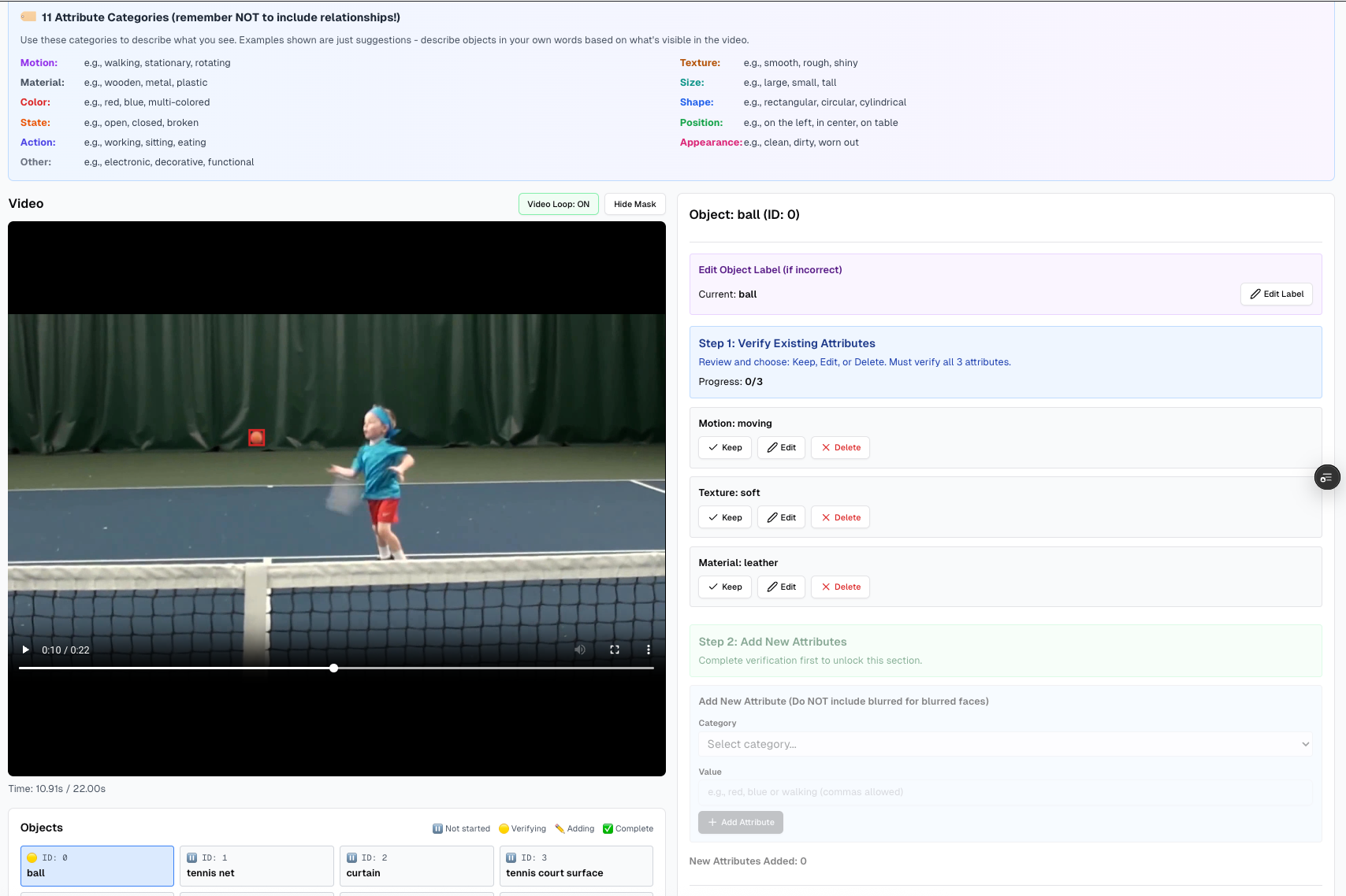
For scene graph annotations, we employ a model-in-the-loop approach. We prompt GPT-5 with human-annotated object labels to generate initial attributes and relationships with timestamps, dividing relationships into spatial and temporal categories. We then use the Prolific crowdsourcing platform to recruit workers who have been identified as experts in video annotation. Annotators review and edit object labels and attributes, choosing to keep, remove, add, or modify each entry. They are required to annotate at least one attribute per object and are compensated based on the number of attributes annotated. For relationships, annotators perform similar edits, removing incorrect relationship labels, fixing mismatched object IDs, or adjusting timestamps. When object IDs or timestamps are incorrect, annotators can select from all available objects in the video or modify the temporal range where the relationship applies. Figures 13–13 show the annotation interfaces used for verification and editing.

Appendix C Model Details

Our proposed TraSeR introduces a trajectory-aligned token arrangement mechanism, designed to map valid tokens according to the pixel regions covered by each object’s trajectory. However, the rearrangement disrupts the original order and spatial layout of the visual tokens. Therefore, for the token sequence associated with each object’s trajectory, we normalize it into the structured format illustrated in Figure 11. Specifically, we prepend a pair of special tokens, <obj_traj_start> and <obj_traj_end>, to explicitly delineate different trajectories. Within each trajectory segment, we insert the textual identifier of the object (i.e., its corresponding text embedding), which matches the object ID used in the video-scene-graph supervision signals. We then continue to leverage the pretrained special tokens from Qwen2.5-VL to separate the visual tokens associated with each object.

During the compression stage via the dual-resampler, the tokens of each object, either as a whole or partitioned into temporal windows, are fed into two resamplers, while the special tokens and object-ID embeddings bypass the resamplers. The output tokens from the object-trajectory resampler are placed first, followed by the tokens produced by the temporal-window resampler for each respective window.

Figure 11: Rearranged object-level token sequence example. We introduce two new special tokens, <obj_traj_start> and <obj_traj_end>, to delimit individual trajectories. Within each trajectory, we explicitly mark the object identity using the text “Object i”, and we continue to use the existing special tokens from the Qwen2.5-VL vocabulary to separate visual tokens.

These operations directly alter the original token-sequence length and positional structure. As a result, we uniformly change all position IDs of tokens input to the LLM module into a one-dimensional index. Given that the visual tokens have already incorporated 3D-RoPE position embeddings within the ViT, and have subsequently undergone window attention and global attention for ontextual interactions, this one-dimensional positional degradation remains acceptable.

Appendix D Training Details

During training, we set the token-arrangement selection threshold $\tau_{\mathrm{eff}}$ to 0.5 to balance contextual coverage and token count. Both resamplers are configured with three layers and 32 learnable queries. We apply RMSNorm both before and after the cross-attention blocks in each layer. The hidden size of each resampler is set to 2048, and the intermediate size of each MLP layer is $4\times 2048$.

We sample video frames at 1 fps and adopt the same resizing strategy as Qwen2.5-VL. The ViT backbone is frozen, while the projector, language model, and the newly introduced resamplers are trained end-to-end. For the temporal-window resampler, each temporal window spans 4 s, meaning that the token groups corresponding to different temporal segments of a trajectory are processed independently. The object-trajectory resampler processes all tokens belonging to each object in a single pass.

We use a warmup ratio of 0.03 and a weight decay of 0.01. Training is performed on 8 H100 GPUs with a batch size of 1 and gradient accumulation steps set to 2.

Appendix E Additional Experiments and Results

E.1 Evaluation details

To ensure a fair comparison across all baseline models, we provide each model with the bounding-box trajectory of every object during evaluation. For each bounding box, we include both its absolute coordinates and normalized relative coordinates, and we explicitly prompt the model with the original frame resolution. For models that support direct video input, for example, Gemini 2.5 Pro, we supply the bounding boxes and their corresponding timestamps computed from frames sampled at 1 fps. For models that do not support video input, such as GPT-4.1 and GPT-5, we instead feed the 1 fps (which is the same as TraSeR inference setting) sampled frames sequentially, alternating each frame with its associated metadata and the bounding-box information of all objects in that frame.

All models use prompts following a unified structural template, and their outputs are constrained using a predefined JSON schema.

E.2 Comparison under different evaluation criteria

Table 10: Comparison results under different evaluation criteria

	Triplet (IoU 0.1)			Relation (IoU 0.1)			Object (Strict)
Model	PVSG	VidOR	SVG2test	PVSG	VidOR	SVG2test	VIPSeg	PVSG	VidOR	SVG2test
API call only
GPT-4.1 [1]	10.3	15.4	6.8	12.3	17.2	8.1	30.0	15.0	26.9	24.9
Gemini-2.5 PRO [11]	12.3	12.8	9.3	13.9	14.3	10.6	28.0	9.2	20.7	23.3
GPT-5 [43]	23.8	25.6	18.9	24.2	28.5	20.5	38.2	20.1	22.2	33.4
Open weights only
Qwen2.5-VL-3B [4]	0.1	0.4	0.3	0.1	0.8	0.6	15.6	2.4	9.5	9.1
MiniCPM-V 4.5 [63]	0.2	5.0	1.3	0.5	6.6	2.7	25.5	0.5	12.0	16.4
InternVL3.5-4B [58]	0.6	2.1	1.0	1.8	2.9	2.1	20.9	2.9	10.6	14.7
GLM-4.1-9B-Thinking [17]	0.7	5.7	2.1	1.5	7.2	3.5	23.2	2.6	10.4	11.7
Qwen3-VL-4B [59]	0.1	1.1	1.1	0.1	1.4	1.9	22.8	4.4	14.2	16.7
Qwen3-VL-4B-Thinking [59]	0.1	3.7	2.0	1.5	5.7	4.2	22.9	0.8	10.7	16.6
Fine-tuned baselines
FT-Qwen2.5-VL-3B (First Bbox)	0.1	3.5	1.2	0.9	10.0	1.9	11.5	5.9	11.7	9.8
FT-Qwen2.5-VL-3B (Bbox Traj.)	2.5	3.5	1.7	6.6	8.4	3.8	11.0	7.5	13.7	13.1
TraSeR	23.8	32.7	18.5	25.4	36.0	20.8	42.1	29.5	31.7	28.8

We report additional results under the different evaluation criteria introduced in Section 5. Table 10 presents triplet and relation recall under a more relaxed temporal IoU threshold of 0.1. For object evaluation, we adopt the Strict criterion, which only counts predictions as correct if they fall into the Identical semantic categories.

As shown in the table, proprietary models perform reasonably well across all tasks, with GPT-5 achieving the strongest overall results among API-access models. In contrast, open-weight VLMs display a substantial performance gap, particularly on triplet and relation prediction, underscoring the inherent difficulty of fine-grained and temporally grounded scene graph extraction for current open-source models.

Our method, however, demonstrates clear and consistent improvements across all benchmarks. Under the relaxed IoU criterion, TraSeR achieves strong triplet and relation performance, surpassing all open-weight baselines by large margins. Under the strict object-level criterion, TraSeR continues to deliver the best performance across all evaluation datasets, and even exceeds proprietary API models in several cases. These results confirm that our trajectory-aligned tokenization and resampler designs significantly enhance fine-grained object grounding and temporal consistency, both of which are critical for accurate video scene graph generation.

E.3 Additional Ablations

Model architecture.

We further investigate the impact of the resampler architecture by varying the number of resampler layers and the number of learnable queries in the temporal-window resampler. All variants are trained for 3 epochs on the SAV subset of SVG2. As shown in Table 12, the performance differences across architectural variants are relatively small. The configuration with three layers and 32 queries achieves slightly better overall results and inference stability.

Table 11: Data scale ablation showing consistent average performance gains as training data increases.

Metric / Data scale	25%	50%	75%	100%
Triplet
PVSG	10.1	12.2	13.7	16.1
VidOR	20.7	20.5	22.4	22.9
SVG2test	17.5	18.9	15.7	16.7
Relation
PVSG	10.8	13.1	15.4	16.9
VidOR	22.9	22.5	24.7	25.0
SVG2test	19.6	20.9	18.3	18.7
Object
PVSG	76.3	76.6	75.5	72.7
VidOR	90.8	91.2	91.1	91.4
VIPSeg	85.7	85.3	85.7	86.5
SVG2test	79.0	79.0	79.1	79.0
Attribute
SVG2test	22.5	22.3	22.9	27.1
Avg Rank	4	3	2	1

Training data scale.

We analyze the effect of training data scale by comparing models trained with 25%, 50%, 75%, and 100% of the data. As shown in Table 11, increasing the amount of training data consistently improves the average performance across most metrics and benchmarks. For triplet and relation prediction, both VidOR and SVG2_test exhibit clear gains as data scale grows, confirming that learning temporal and relational structures benefits strongly from large SVG2 dataset. Attribute prediction on SVG2_test shows the most pronounced improvement, with a substantial jump from 22.3 to 27.1 when using the full dataset. This indicates that our 593K PVD subset in SVG2 provides diverse and high-quality object-level annotations. The overall average rank demonstrates that larger-scale training yields consistently better performance across all evaluation dimensions.

Table 12: Model architecture ablation study. *PVSG results are evaluated on the VidOR subset.

Variants		Triplet		Relation		Object
Depth	# query of TWR	PVSG*	VidOR	PVSG*	VidOR	PVSG*	VidOR
2	16	12.3	15.1	13.5	16.5	81.3	89.9
3	16	12.8	14.2	11.7	15.4	80.1	90.2
2	32	12.0	15.6	14.7	17.5	80.9	90.0
3	32	13.6	15.0	15.6	16.3	79.7	90.2

E.4 End-to-End Evaluation and Generalization to Long Videos

End-to-end evaluation.

All main-paper experiments follow an open-vocabulary VidSGG (OV-VSGGen) protocol where every model (including TraSeR) receives ground-truth panoptic trajectories as input, so that scene-graph generation quality is evaluated independently of upstream segmentation. We also report an end-to-end evaluation of TraSeR in which trajectories are produced entirely by our Phase-1 pipeline: we run SAM2-based panoptic segmentation and online–offline tracking on the test videos, retain pipeline-generated masks whose IoU with any ground-truth instance exceeds 0.3, and feed these matched pipeline masks directly into TraSeR for inference and metric computation.

Table 13 compares the two settings. While the end-to-end variant shows reduced performance (largely because our pipeline achieves AR of $\sim$0.7 on VIPSeg, PVSG, and VidOR (Table 1), leaving a fraction of instances missed or imprecisely delineated), the results nonetheless remain remarkably competitive. TraSeR (end-to-end) still outperforms GPT-4.1 and Gemini-2.5 Pro with ground-truth input on triplet and relation detection across PVSG and SVG2_test, and surpasses both on object prediction and attribute recall. This indicates that our pipeline generates trajectories of sufficient quality to support meaningful, full-scene-graph extraction, and that TraSeR’s trajectory-aligned token arrangement and dual-resampler design are robust to realistic levels of segmentation imperfection. Improving Phase-1 segmentation quality directly translates to better end-to-end scene graph performance.

Table 13: Comparison of TraSeR under two input settings: ground-truth panoptic segmentation masks (TraSeR, used in all main-paper experiments) versus pipeline-generated and IoU-matched ($\geq$0.3) masks (TraSeR (end-to-end)). ^†PVSG is evaluated on its VidOR subset only.

	Triplet			Relation			Object				Attribute
Model	PVSG†	VidOR	SVG2test	PVSG†	VidOR	SVG2test	VIPSeg	PVSG†	VidOR	SVG2test	SVG2test
TraSeR (end-to-end)	10.0	4.3	10.6	13.4	6.1	16.2	72.2	63.4	62.9	64.1	17.6
TraSeR	19.2	22.9	16.7	20.1	25.0	18.7	86.5	81.9	91.4	79.0	27.1

Generalization to long videos.

The PVSG benchmark contains three subsets from distinct video corpora: VidOR (avg. 48s), Epic-Kitchens (avg. 120s), and Ego4D (avg. 166s). These span a range of durations well beyond that of SVG2 training videos. Table 14 therefore serves as a zero-shot temporal generalization evaluation: TraSeR was never explicitly trained on videos longer than $\sim$30s, yet is evaluated on sequences up to $\sim$10$\times$ longer.

The results reveal that object prediction accuracy remains non-trivial across all durations, demonstrating that the object-trajectory resampler’s global aggregation provides a semantically stable representation of object identity even for long trajectories. Relation and triplet performance declines, reflecting the inherent difficulty of fine-grained temporal grounding over extended horizons beyond the training distribution. Our architecture provides controllable scalability: the number of learnable queries and the temporal-window resampler’s window size can be adjusted to better balance coverage and granularity in long videos These results highlight the generalization capability of our model while identifying long-video VSG as a promising direction for future work: explicitly incorporating longer training videos and scalable temporal architectures could substantially close the performance gap at extended durations.

Table 14: Performance of TraSeR across the three PVSG subsets, which span video durations from 48s (VidOR) to 166s (Ego4D). Object prediction remains robust at all durations, while relation and triplet performance decreases for longer videos, motivating future long-video training strategies.

	Triplet			Relation			Object
Model	VidOR (48s)	Epic-Kitchens (120s)	Ego4D (166s)	VidOR (48s)	Epic-Kitchens (120s)	Ego4D (166s)	VidOR (48s)	Epic-Kitchens (120s)	Ego4D (166s)
TraSeR	19.2	6.5	5.1	20.1	7.4	7.7	81.7	63.2	66.0

Figure 12: Crowdworkers editing and annotating objects and attributes from segmentation tracking.

Figure 13: Crowdworkers verifying and fixing relationships.

Table 15: Prompts for Spatial Relationship Extraction.

Table 16: Prompts for Non-Spatial Relationship Extraction.

References

- [1] (2023) Gpt-4 technical report. arXiv preprint arXiv:2303.08774. Cited by: §A.2, Table 10, §3.1, Table 3, §5.
- [2] (2022) Flamingo: a visual language model for few-shot learning. External Links: 2204.14198, Link Cited by: §4.2.
- [3] (2016) Spice: semantic propositional image caption evaluation. In European conference on computer vision, pp. 382–398. Cited by: §1.
- [4] (2025) Qwen2.5-vl technical report. External Links: 2502.13923, Link Cited by: Table 10, §1, Table 3.
- [5] (1987) Recognition-by-components: a theory of human image understanding.. Psychological review 94 (2), pp. 115. Cited by: §1.
- [6] (2017) On the semantics of a glance at a scene. In Perceptual organization, pp. 213–253. Cited by: §1.
- [7] (2025) Perception encoder: the best visual embeddings are not at the output of the network. arXiv:2504.13181. Cited by: §3.2.
- [8] (2025) SAM 3: segment anything with concepts. External Links: 2511.16719, Link Cited by: §3.1.
- [9] (2021) Scene graphs: a survey of generations and applications. arXiv preprint arXiv:2104.01111 2. Cited by: §1.
- [10] (2022) (2.5+ 1) d spatio-temporal scene graphs for video question answering. In Proceedings of the AAAI Conference on Artificial Intelligence, Vol. 36, pp. 444–453. Cited by: §1.
- [11] (2025) Gemini 2.5: pushing the frontier with advanced reasoning, multimodality, long context, and next generation agentic capabilities. External Links: 2507.06261, Link Cited by: Table 10, Table 3, §5.
- [12] (2021-10) Spatial-temporal transformer for dynamic scene graph generation. In Proceedings of the IEEE/CVF International Conference on Computer Vision (ICCV), pp. 16372–16382. Cited by: §2.
- [13] (2022) EPIC-kitchens visor benchmark: video segmentations and object relations. External Links: 2209.13064, Link Cited by: §2.
- [14] (2023) Scenegenie: scene graph guided diffusion models for image synthesis. In Proceedings of the IEEE/CVF International Conference on Computer Vision, pp. 88–98. Cited by: §1.
- [15] (2022) Classification-then-grounding: reformulating video scene graphs as temporal bipartite graphs. In Proceedings of the IEEE/CVF conference on computer vision and pattern recognition, pp. 19497–19506. Cited by: §1.
- [16] (2025) Generate any scene: scene graph driven data synthesis for visual generation training. External Links: 2412.08221, Link Cited by: §1.
- [17] (2024) ChatGLM: a family of large language models from glm-130b to glm-4 all tools. External Links: 2406.12793, Link Cited by: Table 10, §1, Table 3, §5.
- [18] (2022) Ego4D: around the world in 3,000 hours of egocentric video. External Links: 2110.07058, Link Cited by: §2.
- [19] (2023-03) Scene perception and understanding. Oxford University Press. External Links: Document, Link Cited by: §1.
- [20] (2021) Agqa: a benchmark for compositional spatio-temporal reasoning. In Proceedings of the IEEE/CVF Conference on Computer Vision and Pattern Recognition, pp. 11287–11297. Cited by: §1, §1, §1, §3.1, §5.2.
- [21] (2025) Glm-4.1 v-thinking: towards versatile multimodal reasoning with scalable reinforcement learning. arXiv e-prints, pp. arXiv–2507. Cited by: §1.
- [22] (2023) Sugarcrepe: fixing hackable benchmarks for vision-language compositionality. Advances in neural information processing systems 36, pp. 31096–31116. Cited by: §1.
- [23] (2025) SOS: synthetic object segments improve detection, segmentation, and grounding. External Links: 2510.09110, Link Cited by: §1.
- [24] (1992) Dynamic binding in a neural network for shape recognition.. Psychological review 99 (3), pp. 480. Cited by: §1.
- [25] (2020) Action genome: actions as compositions of spatio-temporal scene graphs. In Proceedings of the IEEE/CVF conference on computer vision and pattern recognition, pp. 10236–10247. Cited by: §1, §1, §2, §3.1, Table 2, Table 2.
- [26] (2018) Image generation from scene graphs. In Proceedings of the IEEE conference on computer vision and pattern recognition, pp. 1219–1228. Cited by: §1.
- [27] (2015) Image retrieval using scene graphs. In Proceedings of the IEEE conference on computer vision and pattern recognition, pp. 3668–3678. Cited by: §1.
- [28] (2025) TACS-graphs: traversability-aware consistent scene graphs for ground robot indoor localization and mapping. arXiv preprint arXiv:2506.14178. Cited by: §1.
- [29] (2016) Visual genome: connecting language and vision using crowdsourced dense image annotations. External Links: 1602.07332, Link Cited by: §1, §2.
- [30] (2025) Visual explainable artificial intelligence for graph-based visual question answering and scene graph curation. Visual Computing for Industry, Biomedicine, and Art 8 (1), pp. 9. Cited by: §1.
- [31] (2020) The open images dataset v6. International Journal of Computer Vision. Cited by: §2.
- [32] (2022) Video k-net: a simple, strong, and unified baseline for video segmentation. External Links: 2204.04656, Link Cited by: §2.
- [33] (2025) Unbiased video scene graph generation via visual and semantic dual debiasing. In Proceedings of the Computer Vision and Pattern Recognition Conference, pp. 19047–19056. Cited by: §1.
- [34] (2025) Describe anything: detailed localized image and video captioning. arXiv preprint arXiv:2504.16072. Cited by: §A.2, §3.1, §3.1.
- [35] (2016) Visual relationship detection with language priors. In European Conference on Computer Vision (ECCV), Cited by: §2.
- [36] (2023) Crepe: can vision-language foundation models reason compositionally?. In Proceedings of the IEEE/CVF Conference on Computer Vision and Pattern Recognition, pp. 10910–10921. Cited by: §1.
- [37] (2022-06) Large-scale video panoptic segmentation in the wild: a benchmark. In Proceedings of the IEEE/CVF Conference on Computer Vision and Pattern Recognition (CVPR), pp. 21033–21043. Cited by: Table 1, Table 2, Table 2, §4.3, §5.
- [38] (2021-06) VSPW: a large-scale dataset for video scene parsing in the wild. In Proceedings of the IEEE/CVF Conference on Computer Vision and Pattern Recognition (CVPR), pp. 4133–4143. Cited by: §3.2.
- [39] (2023) Unbiased scene graph generation in videos. External Links: 2304.00733, Link Cited by: §1, §2.
- [40] (2025) HyperGLM: hypergraph for video scene graph generation and anticipation. External Links: 2411.18042, Link Cited by: §1, §2.
- [41] (2024) HIG: hierarchical interlacement graph approach to scene graph generation in video understanding. External Links: 2312.03050, Link Cited by: §2, §2.
- [42] (2024) GPT-4o mini: advancing cost-efficient intelligence. Note: https://openai.com/index/gpt-4o-mini-advancing-cost-efficient-intelligence/Accessed: 2025-02-19 Cited by: §5.
- [43] (2025-08) GPT-5 system card. Technical report OpenAI. External Links: Link Cited by: Table 10, §1, §1, §3.1, Table 3, §5.
- [44] (2025) Synthetic visual genome. External Links: 2506.07643, Link Cited by: §2.
- [45] (2023) Perception test: a diagnostic benchmark for multimodal video models. Advances in Neural Information Processing Systems 36, pp. 42748–42761. Cited by: §1, §5.2.
- [46] (2021) Occluded video instance segmentation: a benchmark. External Links: 2102.01558, Link Cited by: §4.3.
- [47] (2019) Video relation detection with spatio-temporal graph. In Proceedings of the 27th ACM international conference on multimedia, pp. 84–93. Cited by: §2.
- [48] (2023) Virtualhome action genome: a simulated spatio-temporal scene graph dataset with consistent relationship labels. In Proceedings of the IEEE/CVF Winter Conference on Applications of Computer Vision, pp. 3351–3360. Cited by: §1.
- [49] (2024) Sam 2: segment anything in images and videos. arXiv preprint arXiv:2408.00714. Cited by: §A.1.1, §B.3, §1, §3.1, §3.2, §3.2, Table 2.
- [50] (2024) Grounded sam: assembling open-world models for diverse visual tasks. External Links: 2401.14159 Cited by: §A.1.2.
- [51] (2024) Action scene graphs for long-form understanding of egocentric videos. In Proceedings of the IEEE/CVF Conference on Computer Vision and Pattern Recognition, pp. 18622–18632. Cited by: §2.
- [52] (2019) Annotating objects and relations in user-generated videos. In Proceedings of the 2019 on International Conference on Multimedia Retrieval, pp. 279–287. Cited by: §2, Table 1, Table 2, Table 2, §4.3, §5.
- [53] (2017) Video visual relation detection. In Proceedings of the 25th ACM International Conference on Multimedia, pp. 1300–1308. Cited by: §2, §2, Table 2, Table 2, §4.3.
- [54] (2020) Unbiased scene graph generation from biased training. In Proceedings of the IEEE/CVF conference on computer vision and pattern recognition, pp. 3716–3725. Cited by: §1.
- [55] (2021-10) Target adaptive context aggregation for video scene graph generation. In Proceedings of the IEEE/CVF International Conference on Computer Vision (ICCV), pp. 13688–13697. Cited by: §2.
- [56] (2023) Towards open-vocabulary video instance segmentation. External Links: 2304.01715, Link Cited by: §4.3.
- [57] (2024) Qwen2-vl: enhancing vision-language model’s perception of the world at any resolution. External Links: 2409.12191, Link Cited by: §5.
- [58] (2025) InternVL3.5: advancing open-source multimodal models in versatility, reasoning, and efficiency. External Links: 2508.18265, Link Cited by: Table 10, §1, Table 3, §5.
- [59] (2025) Qwen3 technical report. arXiv preprint arXiv:2505.09388. Cited by: Table 10, Table 10, §1, Table 3, Table 3.
- [60] (2022) Panoptic scene graph generation. External Links: 2207.11247, Link Cited by: §2.
- [61] (2023) 4d panoptic scene graph generation. Advances in Neural Information Processing Systems 36, pp. 69692–69705. Cited by: §2.
- [62] (2023) Panoptic video scene graph generation. External Links: 2311.17058, Link Cited by: §1, §2, §2, Table 1, Table 2, Table 2, §5.
- [63] (2024) MiniCPM-v: a gpt-4v level mllm on your phone. External Links: 2408.01800, Link Cited by: Table 10, §1, Table 3, §5.
- [64] (2024) Task me anything. ArXiv abs/2406.11775. External Links: Link Cited by: §1.
- [65] (2024) ProVision: programmatically scaling vision-centric instruction data for multimodal language models. External Links: 2412.07012, Link Cited by: §1.