SOTAlign: Semi-Supervised Alignment of Unimodal
Vision and Language Models via Optimal Transport

Abstract

The Platonic Representation Hypothesis posits that neural networks trained on different modalities converge toward a shared statistical model of the world. Recent work exploits this convergence by aligning frozen pretrained vision and language models with lightweight alignment layers, but typically relies on contrastive losses and millions of paired samples. In this work, we ask whether meaningful alignment can be achieved with substantially less supervision. We introduce a semi-supervised setting in which pretrained unimodal encoders are aligned using a small number of image–text pairs together with large amounts of unpaired data. To address this challenge, we propose SOTAlign, a two-stage framework that first recovers a coarse shared geometry from limited paired data using a linear teacher, then refines the alignment on unpaired samples via an optimal-transport-based divergence that transfers relational structure without overconstraining the target space. Unlike existing semi-supervised methods, SOTAlign effectively leverages unpaired images and text, learning robust joint embeddings across datasets and encoder pairs, and significantly outperforming supervised and semi-supervised baselines.

1 Introduction

Figure 1: Semi-Supervised Vision-Language Alignment. We tackle the alignment of frozen unimodal encoders where paired data (red blocks) is scarce but unpaired data is abundant. The key challenge is: how to define a training signal for unpaired data when ground-truth cross-modal correspondences are missing?

Vision-language models (VLMs) learn a shared embedding space for images and text, enabling zero-shot transfer to unseen concepts and domains. Since CLIP (Radford et al., 2021) and ALIGN (Jia et al., 2021), the dominant paradigm has relied on large-scale contrastive training on paired image-text data, with performance improving predictably as supervision scales. While effective, this approach requires hundreds of millions of paired samples (Cherti et al., 2023), making VLMs costly to train and difficult to adapt when paired data are limited. This issue arises in many critical applications, such as specialized scientific, medical, or industrial domains, where collecting large-scale annotations is expensive, time-consuming, or infeasible.

In this paper, we investigate vision–language alignment beyond large-scale supervision, asking whether meaningful alignment can be achieved from pretrained encoders using only a small number of paired samples together with abundant unimodal data. We posit that, under the Platonic Representation Hypothesis (Huh et al., 2024), unimodal models should already encode compatible semantic structures, making such alignment possible with minimal supervision.

SOTAlign Overview.  We focus on training lightweight alignment layers on top of pretrained unimodal encoders. In this setting, we first demonstrate that meaningful cross-modal alignment can be recovered from very few paired samples using simple linear methods, providing empirical support for the Platonic Representation Hypothesis. Then, we introduce SOTAlign (Semi-supervised Optimal Transport-based Alignment), a simple approach that enables to further refine such alignment by leveraging large unimodal datasets, achieving state-of-the-art results in this semi-supervised setting. SOTAlign relies on KLOT, an optimal-transport-based divergence that enables to transfer the initial geometric structure of the linear teacher while allowing sufficient flexibility to avoid underfitting. Critically, we derive the explicit gradient of KLOT divergence, removing the memory bottlenecks that have limited the scalability of previously optimal-transport-based alignment methods. In the experimental section, we implement strong supervised and semi-supervised baselines and demonstrate the superior performances of SOTAlign across a wide range of downstream tasks. We carefully explore the robustness of SOTAlign to a variety of factors such as the number of paired samples, the number of unimodal samples, and the pretrained unimodal models. Critically, we also show that SOTAlign can leverage samples from multiple sources simultaneously, for example combining unimodal images from ImageNet and captions from CC12M to improve performances on COCO despite a significant distribution shift.

In short, we make the following contributions:

• We show that meaningful vision–language alignment can be recovered from very few paired samples using simple linear methods.

• We introduce SOTAlign, a semi-supervised approach that leverages unpaired unimodal data to achieve state-of-the-art alignment.

• We propose KLOT, a novel optimal-transport-based divergence, and fully address the memory bottlenecks that plagued prior OT-based methods.

• We validate the robustness of SOTAlign through extensive experiments across tasks, datasets, and encoders.

2 Related Work

Vision–Language Models.  VLMs learn a joint embedding space for images and text, enabling zero-shot transfer across downstream tasks. CLIP (Radford et al., 2021) established this paradigm through large-scale contrastive pretraining on 400 million image–text pairs, demonstrating that strong alignment can emerge from frozen pretrained encoders.

Subsequent work has focused on scaling data and refining contrastive objectives to improve performance. ALIGN (Jia et al., 2021) leveraged noisy web-scale supervision, while SigLIP (Zhai et al., 2023) and SigLIPv2 (Tschannen et al., 2025) introduced alternative losses and massive multilingual datasets, with SigLIPv2 training on WebLI, comprising 10 billion images and 12 billion alt-texts across 109 languages. These efforts are consistent with empirical scaling laws observed for CLIP-style models (Cherti et al., 2023), but also highlight a central limitation: achieving state-of-the-art performance requires millions or billions of paired samples, which is impractical in many settings and modalities.

More recently, OT-CLIP (Shi et al., 2024) proposed an Optimal Transport (OT) interpretation of the InfoNCE objective (Oord et al., 2018), viewing contrastive learning as inverse OT with a fixed identity transport plan. We adopt this perspective in the present work, but extend it beyond fully supervised settings by allowing target transport plans that are not restricted to the identity. Moreover, we derive an explicit expression for the gradient of the resulting objective (Theorem 5.1), removing the memory bottlenecks that have limited OT-based approaches to small batch sizes.

The Platonic Representation Hypothesis.  Huh et al. (2024) posit that neural networks trained on different modalities, architectures, or objectives tend to converge toward compatible latent representations that reflect shared underlying structure in the data. In the context of vision-language models, this perspective suggests that pretrained unimodal image and text encoders may already produce semantically aligned representations, even in the absence of explicit cross-modal training. This observation motivates an alternative approach to VLM construction, in which the pretrained encoders are kept frozen and only lightweight alignment layers are learned to reconcile their representation spaces. Several recent works adopt this paradigm, demonstrating that strong vision–language performance can be achieved by aligning frozen pretrained unimodal encoders rather than training multimodal models from scratch (Vouitsis et al., 2024; Zhang et al., 2025a; Maniparambil et al., 2025; Huang et al., 2025). Our work follows this line of research, but focuses on regimes where paired supervision is severely limited.

Low-Supervision Alignment.  A growing body of work has explored alignment under weak, limited, or absent supervision. In unimodal settings, Jha et al. (2025) show that text embeddings can be aligned across representation spaces without paired data. Extending this idea to cross-modal alignment, Maniparambil et al. (2024) and Schnaus et al. (2025) demonstrate that vision–language representations can also be matched without supervision, but rely on quadratic assignment problem solvers that scale only to a few hundred samples, limiting applicability.

Closer to our setting, S-CLIP (Mo et al., 2023) introduces a semi-supervised framework in which optimal transport defines target similarities between unpaired images and paired captions, with promising results for domain adaptation of CLIP. In contrast, we define target similarities even between unpaired images and unpaired captions, enabling effective use of large-scale unimodal data on both sides (Figure 1). SUE (Yacobi et al., 2025) also considers semi-supervised vision–language alignment, but is limited to a single dataset and a single downstream task. Our work generalizes this setting across tasks, datasets, and encoder combinations. Finally, STRUCTURE (Gröger et al., 2025) augments InfoNCE with a regularization term encouraging preservation of unimodal geometry. While evaluated in supervised settings, this idea could in principle leverage unpaired data and is therefore included as a baseline in our experiments.

3 Methodology

Figure 2: SOTAlign is a two-step method for the alignment of pretrained unimodal image and text encoders. First, we fit a linear alignment model only using the limited amount of available image-text pairs. Then, we use this linear model as a teacher to regularize the training of alignment layers $f$ and $g$ for a joint embedding space leveraging unimodal (unpaired) data.

Notations.  For $u,v\in\mathbb{R}^{d}$, we denote the cosine similarity by $k(u,v)=\frac{\langle u,v\rangle}{\left\lVert u\right\rVert\left\lVert v\right\rVert}$. We stack batches of $n$ vectors as matrices in $\mathbb{R}^{n\times d}$. Given $U\in\mathbb{R}^{n\times d}$ and $V\in\mathbb{R}^{m\times d}$, we define the affinity matrix $K[U,V]\in\mathbb{R}^{n\times m}$ with entries

$$K[U,V]_{i,j}=k(U_{i},V_{j}).$$

We define the (row-wise) Softmax normalization as

$$\operatorname{Softmax}_{\varepsilon}(K)_{i,j}=\frac{\exp\!\left(\nicefrac{{K_{i,j}}}{{\varepsilon}}\right)}{\sum_{k=1}^{n}\exp\!\left(\nicefrac{{K_{i,k}}}{{\varepsilon}}\right)}.$$

3.1 Problem Formulation

We denote $d_{x}$ (resp. $d_{y}$) the latent dimension of the pretrained vision (resp. language) encoder. We consider the problem of learning alignment layers $f_{\theta_{1}}:\mathbb{R}^{d_{x}}\rightarrow\mathbb{R}^{d}$ and $g_{\theta_{2}}:\mathbb{R}^{d_{y}}\rightarrow\mathbb{R}^{d}$ that encode vision and language into a shared space of dimension $d$, parametrized by $\theta=(\theta_{1},\theta_{2})$.

In this setting, the training objective is often formulated as minimizing the divergence between the geometry of the shared space and a target geometry. Formally, given a dataset of image and language embeddings $X\in\mathbb{R}^{n\times d_{x}}$ and $Y\in\mathbb{R}^{n\times d_{y}}$, the goal is to minimize

$$\mathcal{L}(\theta;X,Y)=$$ (1)

$$\operatorname{DIV}\!\left(K[f_{\theta_{1}}(X),\,g_{\theta_{2}}(Y)]\,\middle|\middle|\,K^{*}[X,Y]\right),$$

where $K^{*}$ denotes the “target geometry” and $\operatorname{DIV}$ is some divergence between two affinity matrices. In the fully supervised setting, the dataset is made of pairs i.e. $Y_{i}$ is the caption of $X_{i}$ and the target similarity is set to the identity

$$K^{*}[X,Y]=I_{n}.$$ (2)

For instance, the InfoNCE loss (Oord et al., 2018)

$$-\frac{1}{n}\sum_{i=1}^{n}\log\frac{\exp\!\left(K\!\left[f(X),g(Y)\right]_{i,i}\right)}{\sum_{j=1}^{n}\exp\!\left(K\!\left[f(X),g(Y)\right]_{i,j}\right)},$$ (3)

is a special case of (1) for $K^{*}=I_{n}$ and $\operatorname{DIV}\!\left(K\,\middle|\middle|\,K^{*}\right)=\lim_{\varepsilon\to 0}\operatorname{KL}\!\left(\operatorname{Softmax}_{\varepsilon}(K^{*})\,\middle||\,\operatorname{Softmax}_{1}(K)\right)$.

Thus, the main challenge to extend these approaches to unsupervised data is to introduce a target $K^{*}[X,Y]$ that is defined even if we don’t assume that $X$ and $Y$ are pairs.

3.2 Semi-Supervised Setting

We consider a semi-supervised setting with three types of data. First, we observe a small set of paired samples $(A,B)$, where $A\in\mathbb{R}^{n_{p}\times d_{x}}$ and $B\in\mathbb{R}^{n_{p}\times d_{y}}$, and each row of $A$ is aligned with the corresponding row of $B$. In addition, we have access to large collections of unpaired data: unlabeled images $X\in\mathbb{R}^{n_{x}\times d_{x}}$ and unlabeled text $Y\in\mathbb{R}^{n_{y}\times d_{y}}$. Finally, we assume that the number of supervised pairs is limited, i.e., $n_{p}\ll n_{x}$ and $n_{p}\ll n_{y}.$ This setting is motivated by two considerations. First, it allows us to study how far supervision can be reduced while still enabling the recovery of a meaningful alignment between modalities, providing a direct test of the Platonic Representation Hypothesis. Second, such a regime reflects many practical scenarios in multimodal learning, where collecting paired data is expensive or infeasible and only a small number of aligned samples is available.

3.3 SOTAlign

We address this setting with a two step approach:

First, we fit a a simple linear alignment model with the supervised pairs $(A,B)$. We denote $W_{x}\in\mathbb{R}^{d_{x}\times d^{\prime}}$ and $W_{y}\in\mathbb{R}^{d_{y}\times d^{\prime}}$ the linear projections produced by this model. An important finding of this work is that such linear models already yield surprisingly strong alignment. We dedicate Section 4 to this fundamental component of our method.

Then we use this linear model to regularize the training of the final alignment layers $f_{\theta_{1}}$ and $g_{\theta_{2}}$ in a pseudo-labeling fashion. More precisely, we constrain the geometry of the learned shared space to stay close to that produced by the linear teacher. This regularization writes as

$$\Omega(\theta;X,Y)=$$ (4)

$$\operatorname{DIV}\!\left(K\left[f_{\theta_{1}}(X),g_{\theta_{2}}(Y)]\right)\,\middle|\middle|\,K[XW_{x}^{T},YW_{y}^{T}]\right),$$

where the choice of the divergence $\operatorname{DIV}$ is the second core component of the method and is discussed in Section 5.

Finally, our training loss is

$$\mathcal{L}_{\alpha}(\theta;A,B,X,Y)=\mathcal{L}(\theta;A,B)+\alpha\Omega(\theta;X,Y),$$ (5)

where $\alpha$ controls the strength of the regularization.

Algorithm 1 SOTAlign Training

0: $(A,B),X,Y$

1: $(W_{x},Wy)\leftarrow\text{LinearAlignement}(A,B)$

2: Initialize encoders $f$ and $g$

3: for $i=1,\dots,T$ do

4:  Sample $X_{b}\sim X$ # Sample batch of image embeddings

5:  Sample $Y_{b}\sim Y$ # Sample batch of text embeddings

6:  $K^{*}\leftarrow\text{cosine}(X_{b}W_{x}^{\top},Y_{b}W_{y}^{\top})$

7:  $K\leftarrow\text{cosine}(f(X_{b}),g(Y_{b}))$

8:  $K_{p}\leftarrow\text{cosine}(f(A),g(B))$

9:  $\mathcal{L}\leftarrow\operatorname{SigLIP}(K_{p},I_{n_{p}})+\alpha\operatorname{KLOT}(K,K^{*})$

10:  Update $f,g$ using $\nabla\mathcal{L}$

11: end for

4 Linear Alignment Model

The first core component of the proposed method is the linear alignment model. This model is trained with the limited amount of pairs available and then used as a teacher to regularize the training of the full semi-supervised model. As highlighted in the experimental section, such linear models achieve surprisingly strong alignment performances. We now discuss a selection of suitable candidates.

Procrustes Alignment.  In the Orthogonal Procrustes problem, one tries to align two point clouds by looking for the orthogonal transformation that minimizes the RMSE (Schönemann, 1966). We slightly adapt its formulation to our setting by looking for two orthogonal transformations that map the pairs $(A,B)$ to a shared space. Formally,

$$(W_{x},W_{y}) =\arg\max_{P,Q}\,\langle AP^{\top},BQ^{\top}\rangle$$ (6)

$$\text{s.t.}\quad PP^{\top}=QQ^{\top}=I_{d^{\prime}}$$

This formulation assumes that the data is first centered and normalized which is omitted here for the sake of simplicity.

Canonical Correlation Analysis.  In statistics, CCA is used to find a space in which two random variable are maximally correlated which each others (Mardia et al., 2024). Transposing to our setting, the two random variables are the text and image embeddings and CCA writes as

$$(W_{x},W_{y})=\arg\max_{P,Q}\,\langle AP^{\top},BQ^{\top}\rangle$$ (7)

s.t. $$(AP^{\top})^{\top}(AP^{\top})=(BQ^{\top})^{\top}(BQ^{\top})=I_{d^{\prime}}$$

The main difference from Procrustes is that the orthogonality constraint is applied to the shared space directions instead of the transformation itself. The solutions to Equation (6) and (7) are provided in Appendix C.1.

Contrastive Learning.  Finally, perhaps the most natural choice is to consider a linear projection trained with a classical contrastive learning approach, formally

$$(W_{x},W_{y})=\arg\min_{P,Q}\,\operatorname{DIV}\!\left(K[AP^{T},BQ^{T}]\,\middle|\middle|\,I_{n_{p}}\right),$$ (8)

where $\operatorname{DIV}$ is the InfoNCE loss defined in equation (3) or an alternative such as the SigLIP loss (Zhai et al., 2023).

5 Choice of Divergence

The second core component of our method is the choice of a divergence $\operatorname{DIV}\!\left(K\,\middle|\middle|\,K^{\ast}\right)$, where $K,K^{\ast}\in\mathbb{R}^{n\times n}$ denote, respectively, the affinity matrix induced by the trainable shared representation and the target affinity matrix. This section examines several possible choices for this divergence and discusses their respective strengths and limitations.

Centered Kernel Alignment.  One of the most popular ways to compare affinity/kernel matrices is Centered Kernel Alignment (CKA) (Cristianini et al., 2001). Denoting $H=I_{n}-\mathbbm{1}\mathbbm{1}^{T}$, CKA writes as

$$\text{CKA}(K,K^{*})=\frac{\langle KH,HK^{*}\rangle}{\sqrt{\langle KH,HK\rangle\langle K^{*}H,HK^{*}\rangle}}.$$ (9)

CKA admits a linear-time computation in the batch size $n$ when implemented via kernel factorizations (Proposition C.6), which constitutes a non-negligible practical property for alignment methods operating with large batches (Zhang et al., 2025a). However, CKA also suffers from known limitations (Davari et al., 2022) and, more importantly in our setting, enforces a strong constraint of the form $K\approx K^{\ast}$. This can be overly restrictive when $K^{\ast}$ is only intended as a regularizing signal provided by a linear teacher, rather than an exact target geometry.

Generalized InfoNCE.  As highlighted above, it might be beneficial to use a regularization that does not enforce $K$ to be exactly aligned with $K^{*}$. To this end, one can consider the generalized InfoNCE loss (Shi et al., 2024) as it only enforces that $\operatorname*{arg\,max}_{j}K_{i,j}\approx\operatorname*{arg\,max}_{j}K^{*}_{i,j}$. This is achieved by first applying a Softmax on the affinity matrices before comparing them, i.e.,

$$\operatorname{InfoNCE}(K\mid\mid K^{*})=$$ (10)

$$\operatorname{KL}\!\left(\operatorname{Softmax}_{\epsilon^{*}}(K^{*})\,\middle||\,\operatorname{Softmax}_{\epsilon}(K)\right).$$

The classical version is recovered for $\varepsilon^{*}\!\to\!0$ and $K^{*}=I_{n}$.

KLOT.  Given the previous interpretation of InfoNCE, we consider a natural extension that seeks the preservation of the entire Optimal Transport (OT) plan instead of only the nearest neighbor. Introducing $\Pi_{n}=\bigl\{\,P\in\mathbb{R}_{+}^{n\times n}\;\big|\;P\mathbf{1}=\mathbf{1},\;P^{\top}\mathbf{1}=\mathbf{1}\,\bigr\},$ the OT plan is defined as

$$OT_{\epsilon}(K)=\operatorname*{arg\,min}_{P\in\Pi_{n}}-\langle P,K\rangle+\epsilon H(P),$$ (11)

where $H(P)=\langle P,\log P\rangle$ is the negative entropy. Note that it is a natural extension of Softmax as $\operatorname{Softmax}_{\epsilon}(K)=\operatorname*{arg\,min}_{P\mathbf{1}=\mathbf{1}}-\langle P,K\rangle+\epsilon H(P)$ and, similarly to Softmax, setting $\epsilon=0$ recovers a strict one-to-one mapping. More details about OT are available in Appendix C.2.

Then, we define the KLOT divergence as

$$\operatorname{KLOT}(K\mid\mid K^{*})=\operatorname{KL}\!\left(OT_{\epsilon^{*}}(K^{*})\,\middle||\,OT_{\epsilon}(K)\right).$$ (12)

This formulation is similar to that proposed by Van Assel et al. (2023) for the purpose of dimensionality reduction and generalizes (Shi et al., 2024) beyond $K^{*}=I_{n}$.

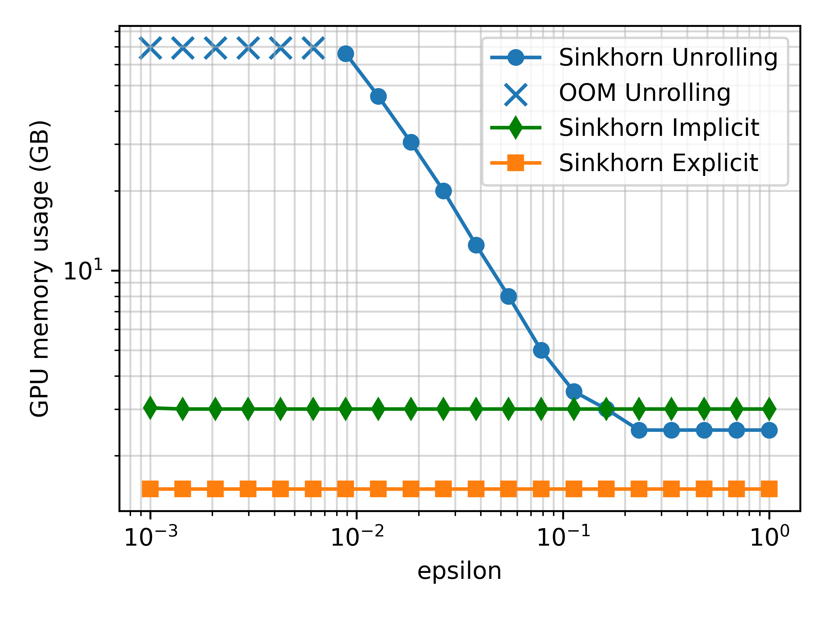
The main limitation of KLOT (5) is that $OT_{\epsilon}(K)$ does not admit a closed-form solution. While the Sinkhorn algorithm (Cuturi, 2013) provides fast convergence on GPUs, computing the gradient $\nabla_{K}OT_{\epsilon}(K)$ remains challenging. Existing approaches rely either on backpropagating through the Sinkhorn iterations by unrolling the algorithm (Genevay et al., 2018), which induces a severe memory bottleneck, or on implicit differentiation techniques (Eisenberger et al., 2022), which significantly increase time complexity. We fully address this limitation by deriving an explicit expression for the gradient (Theorem 5.1).

Theorem 5.1.

For any transport plan $P\in\Pi_{n}$,

$$\nabla_{K}\operatorname{KLOT}(K\mid\mid K^{*})=\frac{\text{OT}_{\epsilon}(K)-\text{OT}_{\epsilon^{*}}(K^{*})}{\epsilon^{*}}.$$ (13)

Proof is provided in Appendix C.2.

As illustrated in Figure 3, our approach removes the memory bottleneck inherent to Sinkhorn unrolling and can be up to $50\times$ faster than implicit differentiation (Figure 6). This is a general result that could potentially apply to a range of OT-based methods using similar objectives, including recent approaches in model alignment and contrastive learning (Van Assel et al., 2023; Mo et al., 2023; Shi et al., 2024).

Figure 3: GPU memory usage for a batchsize $n=10$k when computing the gradient of the OT-based divergence with naive solver unrolling (blue) and the provided explicit gradient formula (orange). Additionnal results are reported in appendix B.1.

6 Experiments

Experimental Setting.  We train all models using a maximum batch size of 32k, composed of up to 10k paired samples and completed with unpaired images and text. We use the LION optimizer (Chen et al., 2023) with a cosine annealing learning-rate schedule, a maximum learning rate of $10^{-4}$, and a weight decay of $10^{-5}$, and train for 2000 iterations. For the supervised component of the loss, we employ the SigLIP objective, initializing the logit scale to $20$ and the logit bias to $-10$, with both parameters learned during training. Unless otherwise specified, we use DINOv3 ViT-L (Siméoni et al., 2025) and NV-Embed-v2 (Lee et al., 2025) as the pretrained vision and language encoders, respectively. By default, experiments are conducted with 10k paired samples and, when applicable, up to 1M unpaired images and texts drawn from CC3M (Sharma et al., 2018). We vary the weight of the regularization in Equation 5 over $\alpha\in\{10^{-3},10^{-4},10^{-5}\}$ and select it based on retrieval performance on CC3M, accounting for different ratios of supervised to unsupervised data. We show in Section 6.2 that comparable results can be obtained with alternative settings.

By default, the metric that we report is the average of the text-to-image (T2I) and image-to-text (I2T) retrieval (Recall@1) performance on the COCO validation set which we denote MeanR@1.

6.1 Ablation Studies

Linear Methods.  SOTAlign employs a linear teacher which can be fit using the methods described in Section 4. We report the standalone zero-shot retrieval performance of these linear models when trained on only 10k image-text pairs from CC3M in the first row of Table 1. Notably, even the closed form models (CCA and Procrustes) reach MeanR@1 scores larger than 21%. The linear contrastive approach (SigLIP loss, SAIL baseline) reaches 24.2% and will serve as the main supervised baseline.

Divergences.  To align the teacher’s affinity matrix with the affinity matrix in the learnable shared space, SOTAlign can utilize any of the three divergences detailed in Section 5. Table 1 displays all combinations of linear methods and divergences. Critically, we observe that the proposed OT-based divergence KLOT systematically outperforms the classical alternatives. The best results is achieved for CCA and KLOT and we select this setting for the next experiments.

Table 1: Comparison of linear methods across different divergences. Zero-shot retrieval on COCO (MeanR@1). “None” indicates the standalone performances of the linear method.

	Linear Method
Divergence	Procrustes	CCA	Contrastive
None	21.1	21.5	24.2
CKA	23.5	23.5	24.2
InfoNCE	23.9	24.1	26.5
KLOT	30.0	30.3	28.5

Figure 4: Left: Effect of the number of paired samples (while fixing 1M unpaired samples). Right: Effect of the number of unpaired samples (while fixing 10k pairs). We report the zero-shot retrieval (MeanR@1) on COCO. More metrics are reported in Appendix B.

6.2 Robustness of SOTAlign

Number of Supervised Pairs.  We first analyze how the number of paired image–text samples affects downstream performance. In this experiment, we fix the amount of unpaired data to 1M images and 1M text samples from CC3M, and vary the number of paired examples from $10^{2}$ to $10^{5}$. Figure 4 reports zero-shot retrieval results. Across all supervision levels, SOTAlign consistently outperforms the supervised SAIL baseline, with gains of up to $+10\%$ accuracy in the intermediate regime between $10^{3}$ and $10^{4}$ pairs. As expected, these gains diminish as the number of paired samples increases, and both methods fail under extremely sparse supervision (100 pairs). Overall, SOTAlign reaches the same performances as SAIL with roughly 4 times less supervision.

Number of Unsupervised Samples.  Next, we investigate the effect of unpaired data on downstream performance. In this experiment, we fix the number of pairs to 10k, and vary the number of additional unpaired image and text samples between $10^{4}$ and $10^{6}$. Figure 4 shows that our method successfully leverages unpaired data for zero-shot retrieval. We observe consistent gains from the unpaired data up to 500k unpaired samples.

Figure 5: Relationship between the total sliced Wasserstein distance between CC3M image/text dataset and unimodal datasets, and the downstream performance of SOTAlign trained on 10k CC3M image–text pairs and up to 1M samples from the corresponding unimodal datasets.

Unsupervised Data Source.  We further evaluate our method in a challenging cross-dataset regime where unpaired images and texts originate from entirely different sources (Table 7). Using a fixed set of 10k paired samples from CC3M, we introduce unpaired unimodal data from CC12M, COCO, and ImageNet-1k, as well as synthetic captions. Despite these shifts in the data distributions, our approach consistently outperforms the supervised baseline. Notably, incorporating ImageNet-1k images improves classification performance, while leveraging COCO samples yields retrieval gains by narrowing the gap to the test distribution. These results demonstrate that our framework can effectively exploit unpaired data even when the visual and textual modalities are drawn from disjoint, heterogeneous corpora.

Quantifying the Distribution Shift.  Motivated by these results, we next seek to quantify the effect of distribution shift and relate it to the observed performance gains. Given a source of unpaired data $\mathcal{D}=(X,Y)$ and the paired dataset $\mathcal{D}_{p}=(A,B)$, we define the distribution shift as

$$\mathrm{d}(\mathcal{D},\mathcal{D}_{p})=\mathrm{SSW}(X,A)+\mathrm{SSW}(Y,B),$$ (14)

where $\mathrm{SSW}$ denotes the Spherical Sliced Wasserstein distance  (Liu et al., 2024), with details in Appendix C.2. We adopt this metric because it is scalable to large datasets, well suited to unit-normalized embeddings, and does not require $X$ and $A$ (or $Y$ and $B$) to be aligned. As shown in Figure 5, this distance strongly correlates with downstream performance: unpaired data that are closer to the paired distribution consistently yield larger performance gains when incorporated during training.

Supervised Data Source.  We next study the impact of the paired data source on SOTAlign performance (Table 2), while fixing the unpaired data to 1M samples from CC3M. Varying the source of the 10k image–text pairs reveals that higher-quality supervision can substantially influence alignment. In particular, using CC3M pairs with synthetic captions yields a notable improvement in retrieval performance (+4.8% T2I R@1), suggesting that cleaner textual supervision better guides the exploitation of noisy unpaired data. While pairs drawn from the larger CC12M corpus improve ImageNet classification, the strongest retrieval performance is obtained when using COCO pairs.

Unimodal Encoders.  In the same vein, we examine the impact of the choice of unimodal encoders on zero-shot classification and retrieval performance. We fix the training data to the standard setting of 10k paired samples and 1M unpaired samples from CC3M, and vary only the vision and language encoders. As reported in Table 3, aligning DINOv3 ViT-L with NV-Embed-v2 yields the strongest downstream performance, achieving 46.1% accuracy on ImageNet and 26.5% T2I R@1 on COCO. Among the evaluated vision models, DINOv3 consistently outperforms earlier variants, which we attribute to its substantially larger pretraining corpus of 1.7 billion images, compared to 142 million for DINOv2. This trend aligns with the Platonic Representation Hypothesis (Huh et al., 2024), which suggests that as models scale in data and capacity, their representation spaces increasingly converge. We hypothesize that this intrinsic convergence reduces the alignment gap between modalities, thereby facilitating semi-supervised alignment with SOTAlign. In Appendix B, we reveal a strong positive correlation between representational similarity and downstream MeanR@1 (Pearson $r=0.83$).

Table 2: SOTAlign compared to supervised SAIL across different paired datasets (10k pairs) and 1M unpaired samples from CC3M. Zero-shot retrieval on COCO (MeanR@1). Green values (+) represent the absolute gain.

Paired data	Method	ImageNet 1K	COCO T2I	COCO I2T
CC3M	SAIL	35.6	21.0	27.4
	SOTAlign	46.1 +10.5	26.5 +5.5	34.1 +6.7
CC3M	SAIL	36.2	28.3	37.2
synthetic	SOTAlign	46.5 +10.3	31.3 +3.0	43.1 +5.9
CC12M	SAIL	38.5	20.1	27.2
	SOTAlign	47.4 +8.9	26.1 +6.0	36.3 +9.1
COCO	SAIL	21.8	30.7	42.4
	SOTAlign	35.8 +14.0	34.8 +4.1	46.7 +4.3

Table 3: SOTAlign trained on 10k pairs and 1M unpaired samples from CC3M with different unimodal encoders. Zero-shot classification (top-1 acc) and retrieval (R@1). Green values represent the absolute gain over supervised SAIL.

Vision Model	Language Model	ImageNet 1K	COCO T2I	COCO I2T
DINOv2	Nemotron-8B	32.4 +6.9	15.5 +3.8	23.3 +5.3
	Qwen3-8B	39.5 +7.7	20.9 +4.1	31.1 +7.3
	NV-Embed-v2	42.5 +9.8	23.1 +4.1	31.1 +7.7
DINOv3	Nemotron-8B	35.5 +10.1	16.6 +3.8	26.2 +5.2
	Qwen3-8B	42.7 +9.3	24.1 +5.0	35.3 +7.3
	NV-Embed-v2	46.1 +10.5	26.5 +5.5	34.1 +6.7

6.3 Benchmarking Semi-Supervised Alignment

Baselines.  Since the semi-supervised alignment setting we consider is relatively unexplored, there are no established standard baselines. We therefore compare SOTAlign against a range of supervised and semi-supervised methods which we adapt to our setting. The primary supervised baseline is SAIL (Zhang et al., 2025a), trained on paired image–text data with a SigLIP loss; we also propose a semi-supervised variant that incorporates unpaired samples as additional negatives. We further consider STRUCTURE (Gröger et al., 2025), which regularizes joint embeddings to preserve unimodal geometry, and evaluate this term using either paired data only or both paired and unpaired samples. In addition, we include pseudo-labeling approaches that construct synthetic pairs from similarity distributions, including NNCLR (Dwibedi et al., 2021) (as used in DeCLIP (Li et al., 2022)) and S-CLIP (Mo et al., 2023). Finally, we compare against SUE (Yacobi et al., 2025), a semi-supervised alignment method restricted to retrieval on a single dataset. Full details of all baselines are provided in Appendix A.2.

Table 4: Zero-shot image-text retrieval (Recall@1) on COCO and Flickr30. Comparison of supervised and semi-supervised methods trained with 10k image-text pairs and 1M unpaired samples from CC3M. Upper bound with 1M supervised pairs in grey.

		COCO		Flickr30k
	Method	T2I	I2T	T2I	I2T
Sup.	gray!20SAIL (1M)	gray!2035.5	gray!2045.5	gray!2063.1	gray!2075.0
	SAIL	21.0	27.4	45.7	54.1
	STRUCTURE	21.0	28.7	46.8	54.0
Semi-sup.	SAIL	20.7	26.5	44.9	53.1
	STRUCTURE	20.9	28.0	45.7	56.0
	NNCLR	21.3	27.9	46.6	53.0
	S-CLIP	20.4	27.8	44.5	52.6
	SOTAlign (Ours)	26.5	34.1	51.7	60.8

Table 5: Zero-shot image classification (top-1 accuracy). Comparison of supervised and semi-supervised methods trained with 10k image-text pairs and 1M unpaired samples from CC3M. Upper bound with 1M supervised pairs in grey.

	Method	Food-101	CIFAR-10	CIFAR-100	DTD	ImageNet
Sup.	gray!20SAIL (1M)	gray!2063.9	gray!2097.8	gray!2082.3	gray!2053.5	gray!2056.4
	SAIL	36.4	96.2	71.2	36.8	35.6
	STRUCTURE	38.5	96.7	72.2	39.5	38.2
Semi-sup.	SAIL	36.5	96.2	71.3	35.9	35.6
	STRUCTURE	37.6	96.5	70.8	38.7	36.8
	NNCLR	37.9	96.5	73.0	38.8	37.4
	S-CLIP	35.3	95.9	69.3	37.6	36.4
	SOTAlign (Ours)	50.0	97.5	78.3	42.4	46.1

Zero-Shot Image-Text Retrieval.  We evaluate SOTAlign against these baselines in T2I and I2T retrieval on COCO (Lin et al., 2014) and Flickr30k (Plummer et al., 2015), and report the results in Table 4. In the low-resource regime with 10k image-text pairs, the supervised baseline SAIL reaches 21.0 T2I R@1 and 27.4 I2T R@1. STRUCTURE performs marginally better benefiting from its structure-preservation objective. However, both methods fail to exploit unpaired data, either as additional negatives or for structure preservation. Notably, even the adapted semi-supervised approaches, NNCLR and S-CLIP, are unable to successfully exploit unpaired data. S-CLIP has been originally developed for domain adaptation and appears less robust when confronted with the large diversity of unpaired samples in our setting. Its pseudo-labels are further limited to the small set of paired instances. In contrast, SOTAlign successfully leverages the 1M unpaired images and text from CC3M to improve cross-modal alignment. On Flickr30k, our method reaches 51.7 T2I R@1 and 60.8 I2T R@1, yielding gains of +4.9 and +4.8 over the strongest baselines, respectively. For comparison, we include in gray the supervised upper bound obtained by training SAIL with 1M paired examples.

Zero-Shot Image Classification.  We further evaluate SOTAlign in zero-shot classification on ImageNet (Deng et al., 2009) and more fine-grained classification datasets. The results are displayed in Table 5 and mirror the trends observed in zero-shot retrieval. STRUCTURE outperforms SAIL in the supervised setting, but is not able to leverage unpaired data for additional performance gains. Existing semi-supervised methods like NNCLR and S-CLIP do not show any improvements over the supervised baselines. Only SOTAlign is able to leverage 1M unpaired samples during alignment to improve zero-shot image classification. Our method achieves an ImageNet top-1 accuracy of 46.1%, which is an improvement of +7.9 over the best baseline. In grey we display the supervised SAIL baseline trained on 1M image-text pairs as an upper bound.

Alignment per Dataset.  Yacobi et al. (2025) study semi-supervised vision–language alignment using pretrained encoders, but under a substantially simpler setting than ours: their method operates within a single dataset, with paired and unpaired samples drawn from the same distribution and evaluation restricted to retrieval on small test splits (400 samples). In contrast, our setting involves cross-dataset unpaired data and multiple downstream tasks. Nevertheless, when evaluated in their setting, SOTAlign consistently outperforms SUE (Yacobi et al., 2025) and its baselines, achieving gains of +14.3 I2T R@5 on COCO, +40.0 on Flickr30k, and +32.5 on Polyvore (see Table 6).

Table 6: Alignment per dataset. Following the setup of SUE (Yacobi et al., 2025), we train for alignment per dataset and evaluate image-text retrieval (Recall@5).

	COCO		Flickr30k		Polyvore
	100 Pairs		500 Pairs		500 Pairs
Method	I2T	T2I	I2T	T2I	I2T	T2I
CSA	1.3	1.0	1.3	0.8	1.3	1.0
Contrastive	8.5	5.8	9.5	9.8	13.8	11.5
SUE	21.5	18.3	19.8	22.0	22.8	20.8
SOTAlign (Ours)	35.8	35.0	59.8	63.3	55.3	55.3

7 Conclusion

In this work, we introduced a semi-supervised setting for aligning pretrained unimodal encoders, which we believe is relevant to many real-world modalities where large-scale paired data are scarce. We argue that Vision–Language alignment provides an ideal testbed for this problem, as abundant paired data enable systematic exploration of different supervision regimes. To the best of our knowledge, SOTAlign is the first model that can effectively leverage large-scale unimodal data for multi-modal alignment in this setting. We hope that the simplicity of SOTAlign will inspire future work on multi-modal representation alignment beyond fully supervised regimes.

Impact Statement

This work aims to advance research in machine learning, particularly in the study of multimodal representation alignment. While improved alignment methods may have broad downstream applications, we do not identify any specific societal impacts that require explicit discussion here.

Appendix A Experimental Setting

We outline the experimental setup in Section 6.3. Here, we provide further details on our implementation and baselines.

A.1 Implementation Details

Following Zhang et al. (2025a), we create global image representations by concatenating the [CLS] token with the mean of the remaining patch tokens. Text features are computed by averaging all patch tokens. We project both modalities into a shared embedding space of dimensionality $d=1024$ using linear layers $f$ and $g$. We found them to be more robust in our low-supervision regime compared to non-linear layers.

When performing CCA, we add a regularization $\lambda=0.1$ to the eigenvalues of matrices that need to be inverted. Our divergence, KLOT, is computed using the Sinkhorn algorithm with $n=100$ iterations in both spaces. We set the entropic regularization to $\epsilon=0.01$ in the reference space and $\epsilon=0.05$ in the joint embedding space.

Our experiments are conducted with 10k paired samples and, when applicable, up to 1M unpaired images and texts drawn from CC3M (Sharma et al., 2018). We train all models using a maximum batch size of 32k, composed of up to 10k paired samples and completed with unpaired images and text. If there are less than 32k total samples available in our robustness studies, we adjust the batch size accordingly. We use the LION optimizer (Chen et al., 2023) with a cosine annealing learning-rate schedule, a maximum learning rate of $10^{-4}$, and a weight decay of $10^{-5}$, and train for 2000 iterations.

We mainly employ DINOv3 ViT-L (Siméoni et al., 2025) and NV-Embed-v2 (Lee et al., 2025) as the pretrained vision and language encoders, respectively. In Section 6.2, we additionally evaluate SOTAlign with DINOv2 ViT-L (Oquab et al., 2024), Qwen3-Embedding-8B (Zhang et al., 2025b), and Llama-Embed-Nemotron-8B (Babakhin et al., 2025). All of these language models are among the top performing models in the MMTEB benchmark (Enevoldsen et al., 2025).

Our main evaluation metric is the average of the text-to-image (T2I) and image-to-text (I2T) retrieval (Recall@1) performance on the COCO validation set which we denote MeanR@1. Whenever required, we use a similar score on the CC3M validation split for hyperparameter selection.

All experiments can be run on a single A100 GPU with 80 GB memory.

A.2 Baselines

In Section Section 6.3, we compare SOTAlign against several supervised and semi-supervised baselines in zero-shot image classification and retrieval. For each baseline, we consider various configurations as detailed below, and report their optimal performance after hyperparameter tuning.

SAIL (Zhang et al., 2025a) performs contrastive learning of alignment layers with the SigLIP (Zhai et al., 2023) loss exclusively on paired data. This method represents a series of recent supervised contrastive methods for the alignment of pretrained unimodal vision and language models (Vouitsis et al., 2024; Maniparambil et al., 2025; Huang et al., 2025). Following Zhang et al. (2025a), we initialize the logit scale to $20$ and the logit bias to $-10$ and allow both parameters to be trained. We examine the extension of SAIL to our semi-supervised setting by incorporating unpaired samples as additional negatives in the SigLIP loss.

STRUCTURE (Gröger et al., 2025) aligns pretrained encoders in low-resource regimes by augmenting the contrastive objective with an additional loss that forces the similarity distribution in the joint embedding space to lie between the unimodal similarity distributions. While STRUCTURE focuses on a fully supervised setting with paired data, we also evaluate the strength of its regularization term on unpaired data in our semi-supervised setting. We set the number of levels to 1 and the temperature in the softmax function to $\tau=0.07$. We tune the weight of the structure preservation term over $\lambda\in\{0.1,1,10,100,1000\}$, and consider both no warmup and a 500-step warmup schedule.

Further semi-supervised techniques can be borrowed from contrastive pretraining and low-resource domain adaptation to construct pseudo-pairs based on similarity distributions in the unimodal or joint embedding spaces.

NNCLR (Dwibedi et al., 2021) enriches contrastive learning by retrieving the nearest-neighbors of an instance and using them as additional positives. DeCLIP (Li et al., 2022) has adopted such nearest-neighbor supervision in image-language pre-training. We follow this line of work and utilize unpaired images and text as augmentation for the few paired samples. Specifically, for a given image, we find the closest neighbor of its paired caption in the unimodal language space, which then serves as an additional positive for the image. Similarly, for a given text, we find the closest neighbor of its paired image in the unimodal vision space, and can use it as an additional positive for the text. While NNCLR is often implemented with a queue containing the last few batches during training, we can compute the nearest neighbors for all CC3M samples in the unimodal spaces a priori since we utilize pretrained encoders. When training the alignment layers, we then randomly sample a nearest neighbor from the top $k\in\{1,5,10\}$ neighbors, and further perform hyperparameter search for the weights of the contrastive losses with the additional positives: $w_{\text{img}},w_{\text{text}}\in\{0,0.1,1,10\}$.

S-CLIP (Mo et al., 2023) addresses the domain adaption of CLIP with pseudo-labeling at the caption and keyword level. We evaluate their caption-level supervision in our setting. Given an unpaired image, S-CLIP computes similarity scores to paired images, and then uses the resulting similarity distribution to determine pseudo positives from the paired text. The pseudo-positives can be chosen in a hard assignment as the single nearest neighbor (argmax of the distribution, similar to NNCLR) or in a soft assignment as a weighted average of representations. A key component of S-CLIP is its use of OT to find the optimal matching between unpaired and paired images. The method is limited by the small pool of positives. We apply S-CLIP in the unimodal vision and language spaces as well as in the joint-embedding space. We search for pseudo-labels for both unpaired images as well as unpaired text and tune their corresponding weights in the final objective via a grid search: $w_{\text{img}},w_{\text{text}}\in\{0,0.1,1,10\}$.

SUE (Yacobi et al., 2025) studies the alignment of unimodal encoders on a single image-text dataset. Their approach combines learnable spectral embeddings on unpaired data, with CCA on paired data for linear alignment, and a residual network to further refine the alignment.

A.3 Datasets

We construct our semi-supervised setting primarily using CC3M (Sharma et al., 2018) with both raw web captions and synthetic captions generated by DreamLIP (Zheng et al., 2024). We further experiment with disjoint images and texts from CC12M (Changpinyo et al., 2021), COCO (Lin et al., 2014), ImageNet (Deng et al., 2009), and WikiText (Merity et al., 2016). We select models based on their average text-to-image (T2I) and image-to-text (I2T) retrieval performance on the CC3M validation set.

In Section 6.3, we evaluate our model in a zero-shot setting across a diverse suite of classification and retrieval benchmarks.

• Classification: ImageNet (Deng et al., 2009), Food-101 (Bossard et al., 2014), CIFAR-10 (Krizhevsky, 2009), CIFAR-100 (Krizhevsky, 2009), Aircraft (Maji et al., 2013), DTD (Cimpoi et al., 2014), Flowers (Nilsback & Zisserman, 2008)

• Retrieval (T2I, I2T): COCO (Lin et al., 2014), Flickr30 (Plummer et al., 2015)

Appendix B Additional Experiments

B.1 Sinkhorn Backpropagation

The Sinkhorn algorithm has recently been used as a differentiable layer in a wide range of applications, including reinforcement learning (Emami & Ranka, 2018), learning to rank (Adams & Zemel, 2011), discriminant analysis (Flamary et al., 2018), graph matching (Krzakala et al., 2025), and representation learning (Van Assel et al., 2023). Closer to our setting, several recent works have applied Sinkhorn-based objectives to contrastive learning for vision–language models (Mo et al., 2023; Shi et al., 2024).

While the Sinkhorn algorithm (defined in Appendix C.2) is differentiable in theory, computing its gradient in practice is challenging. The most common approach consists in unrolling the Sinkhorn iterations and directly backpropagating through the solver. However, this strategy incurs a large memory overhead, as the full computational graph must be retained for all iterations, causing memory consumption to grow rapidly with the number of Sinkhorn steps.

An alternative is to rely on implicit differentiation, which amounts to solving the linear system defined by the optimality conditions of the entropic OT problem. In the case of Sinkhorn, this system exhibits a particular structure that enables more efficient solvers (Cuturi et al., 2020; Eisenberger et al., 2022). While this approach alleviates the memory explosion associated with unrolling, it remains computationally expensive in practice.

In the context of our proposed divergence,

$$\operatorname{KLOT}(K\mid\mid K^{*})=\operatorname{KL}\!\left(OT_{\epsilon^{*}}(K^{*})\,\middle||\,OT_{\epsilon}(K)\right),$$ (15)

a naive application of the chain rule would suggest that computing the gradient

$$\nabla_{K}\operatorname{KLOT}(K\mid\mid K^{*})$$

requires explicitly forming the Jacobian

$$\frac{\partial\,OT_{\epsilon}(K)}{\partial K},$$

thereby necessitating either Sinkhorn unrolling or implicit differentiation.

Crucially, Theorem 5.1 shows that this is not required. Instead, the gradient of $\operatorname{KLOT}$ admits a closed-form expression that can be computed directly, without evaluating the Jacobian of the Sinkhorn operator.

To empirically illustrate the efficiency of this result, we extract an $n\times n$ affinity matrix with $n=10\text{k}$ from a checkpoint of SAIL training and compare three strategies for computing $\nabla_{K}\operatorname{KLOT}(K\mid\mid K^{*})$: Sinkhorn unrolling, implicit differentiation, and our closed-form gradient. The results are reported in Figure 6. Our approach significantly outperforms both alternatives in terms of memory usage and runtime. In particular, depending on the value of $\epsilon$, which controls the number of Sinkhorn iterations (with convergence scaling as $\mathcal{O}(1/\epsilon^{2})$), the proposed method can be up to $100\times$ more memory efficient than unrolling and up to $50\times$ faster than implicit differentiation.

Figure 6: Comparison of memory usage, runtime, and number of Sinkhorn iterations for different gradient computation strategies. We run as many Sinkhorn iterations as required to achieve marginal convergence within a tolerance of $10^{-6}$.

B.2 Robustness of SOTAlign

In Section 6.2, we analyze the robustness of SOTAlign to variations in both the amount and the source of supervised and unsupervised data. Here, we report the full set of results.

Figure 7 shows how zero-shot classification and retrieval performance vary as a function of the number of paired samples used during alignment. Figure 8 illustrates the effect of increasing the number of unpaired samples, in comparison to the supervised SAIL baseline. Table 8 reports zero-shot classification and retrieval results for different combinations of unimodal vision and language encoders, along with absolute gains over supervised SAIL. Finally, Figure 9 relates these performances to the mutual $k$-NN similarity between encoder pairs, revealing a strong correlation ($r=0.83$), although additional data points will be required to draw firm conclusions.

B.3 Benchmarking Semi-Supervised Alignment

Table 9 reports retrieval performance on COCO and Flickr30k, while Table 10 presents zero-shot image classification accuracy across a variety of downstream datasets.

In Section 6.3, we evaluate SOTAlign in a semi-supervised alignment setting proposed by Yacobi et al. (2025). We train for alignment on a single dataset, and evaluate retrieval on the test split of the same dataset (with only 400 test instances for retrieval). The datasets are: COCO (Lin et al., 2014), Flickr30k (Plummer et al., 2015), and Polyvore (Han et al., 2017). Yacobi et al. (2025) use MLPs for alignment and an embedding dimensionality of 8. In Table 11, we report the performance of SOTAlign adhering to their architectural choices. Our method achieves gains of +5.5 on COCO, +28.7 on Flickr30k, and +18.2 on Polyvore I2T R@5. However, if we lift these constraints and instead use linear alignment layers with a target dimension of 512, performance increases further, reaching +14.3 on COCO, +40.0 on Flickr30k, and +32.5 on Polyvore.

B.4 Quantifying the distribution shift

We study the effect of the distribution shift arising from the use of unpaired data $(X,Y)$ drawn from different sources from those of the paired data $(A,B)$ using the total spherical sliced Wasserstein distance (see Appendix C.2) computed using the Python library POT (Flamary et al., 2021, 2024). In all experiments, we set $p=2$ and use $N=500$ projection directions. Distances between unimodal datasets are reported in Figure 12 averaged over $20$ random seeds corresponding to a different subset of $100\,000$ samples of the dataset and projection set. All distances are computed between embeddings from Dinov3 and NV-Embed-V2 for images and text respectively.

In Figure 5 we exhibit a strong correlation between distance and performance, which provides a good proxy for performance that can be computed without any training or inference. In addition, this correlation is even stronger when one of the unimodal unpaired dataset is fixed to be CC3M and the other is varied. We show that performance is strongly correlated with the SSW distances between the unimodal datasets, $SSW(B,Y)$ and $SSW(A,X)$ in Figure 10 and 11 respectively.

(a) ImageNet classification

(b) COCO T2I retrieval

(c) COCO I2T retrieval

Figure 7: Effect of the number of paired samples during alignment on downstream zero-shot classification and retrieval. We fix 1M unpaired samples from CC3M and vary the number of paired samples.

(a) ImageNet classification

(b) COCO T2I

(c) COCO I2T

Figure 8: Effect of the number of unpaired samples during alignment on downstream zero-shot classification and retrieval. We fix 10k paired samples from CC3M and vary the number of unpaired samples.

Table 7: We train SOTAlign on 10k image-text pairs from CC3M and up to 1M samples from varying unimodal datasets and report the zero-shot classification (top-1 accuracy) and retrieval (R@1). For comparison we report SAIL trained with as many samples and SAIL 1M i.e. the version trained using 1M supervised samples from CC3M (100x more supervision).

Method	Unpaired Images	Unpaired Text	ImageNet-1K	COCO T2I	COCO I2T
gray!20SAIL 1M	gray!20—	gray!20—	gray!20 56.4	gray!20 35.5	gray!20 45.5
SAIL	—	—	35.6	21.0	27.4
SOTAlign	CC3M	CC3M	46.1	26.5	34.1
SOTAlign	CC3M	CC3M synth.	46.2	30.4	39.7
SOTAlign	CC3M	CC12M	44.6	24.5	32.0
SOTAlign	CC12M	CC3M	43.8	24.9	32.8
SOTAlign	CC12M	CC12M	46.8	25.7	34.4
SOTAlign	ImageNet	CC3M	43.4	23.8	31.5
SOTAlign	ImageNet	CC12M	44.3	24.2	31.5
SOTAlign	CC3M	COCO	38.4	28.4	26.7
SOTAlign	CC12M	COCO	38.3	27.7	30.6
SOTAlign	ImageNet	COCO	40.6	25.5	26.1
SOTAlign	COCO	CC3M	38.0	21.7	33.9
SOTAlign	COCO	CC12M	38.5	22.0	33.1
SOTAlign	CC3M	WikiText103	39.8	21.4	27.8
SOTAlign	COCO	WikiText103	37.1	19.5	29.4
SOTAlign	ImageNet	WikiText103	40.7	20.7	28.1

Table 8: SOTAlign trained on 10k pairs and 1M unpaired samples from CC3M with different unimodal encoders. Zero-shot classification (top-1 accuracy) and retrieval (R@1). Green values represent the absolute gain over supervised SAIL.

Vision	Language	Mutual k-NN	Method	ImageNet	COCO	COCO
Model	Model			1K	T2I	I2T
DINOv2	Nemotron-8B	14.6	SAIL	25.5	11.7	18.0
			SOTAlign	32.4 +6.9	15.5 +3.8	23.3 +5.3
	Qwen3-8B	18.9	SAIL	31.8	16.8	23.8
			SOTAlign	39.5 +7.7	20.9 +4.1	31.1 +7.3
	NV-Embed-v2	18.2	SAIL	32.7	19.0	23.4
			SOTAlign	42.5 +9.8	23.1 +4.1	31.1 +7.7
DINOv3	Nemotron-8B	14.1	SAIL	25.4	12.8	21.0
			SOTAlign	35.5 +10.1	16.6 +3.8	26.2 +5.2
	Qwen3-8B	18.0	SAIL	33.4	19.1	28.0
			SOTAlign	42.7 +9.3	24.1 +5.0	35.3 +7.3
	NV-Embed-v2	17.6	SAIL	35.6	21.0	27.4
			SOTAlign	46.1 +10.5	26.5 +5.5	34.1 +6.7

Table 9: Zero-shot text-image retrieval (Recall@K) on COCO and Flickr30k. Comparison of supervised and semi-supervised methods trained with 10k image-text pairs and 1M unpaired samples from CC3M. Upper bound with 1M supervised pairs in grey.

		COCO				Flickr30k
	Method	T2I		I2T		T2I		I2T
		R@1	R@5	R@1	R@5	R@1	R@5	R@1	R@5
Sup.	gray!20SAIL (1M)	gray!2035.5	gray!2061.0	gray!2045.5	gray!2072.0	gray!2063.1	gray!2087.2	gray!2075.0	gray!2094.4
	SAIL	21.0	44.3	27.4	51.7	45.7	75.1	54.1	81.2
	STRUCTURE	21.0	43.7	28.7	52.7	46.8	74.9	54.0	82.9
Semi-sup.	SAIL	20.7	43.6	26.5	51.7	44.9	74.2	53.1	82.1
	STRUCTURE	20.9	43.5	28.0	52.2	45.7	74.9	56.0	83.3
	NNCLR	21.3	44.4	27.9	52.2	46.6	75.3	52.9	82.1
	S-CLIP	20.4	42.6	27.8	50.5	44.5	74.4	52.6	82.3
	SOTAlign (Ours)	26.5	49.8	34.1	59.4	51.7	79.2	60.8	85.7

Figure 9: (R@1COCO) vs mutual k-NN.

Table 10: Zero-shot image classification (top-1 accuracy). Comparison of supervised and semi-supervised methods trained with 10k image-text pairs and 1M unpaired samples from CC3M. Upper bound with 1M supervised pairs in grey..

	Method	Food-101	CIFAR-10	CIFAR-100	Aircraft	DTD	Flowers	ImageNet
Sup.	gray!20SAIL (1M)	gray!2063.9	gray!2097.8	gray!2082.3	gray!209.7	gray!2053.5	gray!2047.2	gray!2056.4
	SAIL	36.4	96.2	71.2	3.9	36.8	24.1	35.6
	STRUCTURE	38.5	96.7	72.2	5.4	39.5	23.6	38.2
Semi-sup.	SAIL	36.5	96.2	71.3	3.8	35.9	21.1	35.6
	STRUCTURE	37.6	96.5	70.8	4.9	38.7	23.2	36.8
	NNCLR	37.9	96.5	73.0	3.8	38.8	24.6	37.4
	S-CLIP	35.3	95.9	69.3	4.4	37.6	22.5	36.4
	SOTAlign (Ours)	50.0	97.5	78.3	5.0	42.4	30.1	46.1

Table 11: Alignment per dataset. Following the setup of SUE (Yacobi et al., 2025), we train for alignment per dataset and evaluate image-text retrieval (Recall@5). We report SOTAlign results adhering to the architectural choices of SUE (MLP, embedding dimensionality of 8) and without these constraints.

	COCO		Flickr30k		Polyvore
	100 Pairs		500 Pairs		500 Pairs
Method	I2T	T2I	I2T	T2I	I2T	T2I
CSA	1.3	1.0	1.3	0.8	1.3	1.0
Contrastive	8.5	5.8	9.5	9.8	13.8	11.5
SUE	21.5	18.3	19.8	22.0	22.8	20.8
SOTAlign (with SUE constraints)	27.0	28.8	48.5	48.8	41.0	39.8
SOTAlign (without SUE constraints)	35.8	35.0	59.8	63.3	55.3	55.3

Figure 10: Performance when using CC3M as paired data, CC3M text as unpaired text, and other image datasets as unpaired images, together with a comparison to the spherical sliced Wasserstein distance between CC3M image and the other image datasets.

Figure 11: Performance when using CC3M as paired data, CC3M text as unpaired text, and other image datasets as unpaired images, together with a comparison to the spherical sliced Wasserstein distance between CC3M image and the other image datasets.

Figure 12: Spherical sliced Wasserstein distances between different image datasets (left) and text datasets (right). We report mean and std of the distances over $20$ seeds.

Appendix C Mathematical Details

C.1 Linear Alignment Models

We now provide the closed-form solutions for the proposed linear alignment models.

Procrustes.

The classical Orthogonal Procrustes problem is defined for two point clouds $A,B\in\mathbb{R}^{n\times d}$ and seeks an orthogonal transformation that best aligns $A$ to $B$. It can be written as

$$\max_{P\in\mathbb{R}^{d\times d}}\;\langle PA^{\top},B\rangle\quad\text{s.t. }PP^{\top}=I_{d}.$$ (16)

This formulation learns a single linear mapping from $A$ to $B$ and implicitly assumes that both point clouds lie in the same ambient space $\mathbb{R}^{d}$.

However, Procrustes alignment is known to admit flexible generalizations beyond this setting (Gower & Dijksterhuis, 2004). In particular, it can be extended to handle representations of different dimensionalities and to learn projections into a shared lower-dimensional space. We now introduce a natural variant of Procrustes alignment that is better suited to our setting.

Proposition C.1 (Closed form solution of Procrustes Alignment).

Let $A\in\mathbb{R}^{n\times d_{a}}$ and $B\in\mathbb{R}^{n\times d_{b}}$, and let $d^{\prime}\leq\min\{d_{a},d_{b}\}$. Consider the optimization problem

$$\max_{P\in\mathbb{R}^{d^{\prime}\times d_{a}},\,Q\in\mathbb{R}^{d^{\prime}\times d_{b}}}\;\langle PA^{\top},BQ^{\top}\rangle\quad\text{s.t. }PP^{\top}=I_{d^{\prime}},\;QQ^{\top}=I_{d^{\prime}}.$$ (17)

Let the singular value decomposition of $A^{\top}B$ be

$$A^{\top}B=U\Sigma V^{\top},$$

with singular values in non-increasing order. Then an optimal solution is given by

$$W_{x}=U_{:,1:d^{\prime}},\qquad W_{y}=V_{:,1:d^{\prime}}.$$

Proof.

We introduce the change of variables

$$\tilde{P}=PU,\qquad\tilde{Q}=QV.$$

Since $U$ and $V$ are orthogonal, $\tilde{P}$ and $\tilde{Q}$ also satisfy $\tilde{P}\tilde{P}^{\top}=\tilde{Q}\tilde{Q}^{\top}=I_{d^{\prime}}$. Using invariance of the Frobenius inner product under orthogonal transformations, the objective rewrites as

$$\langle PA^{\top},BQ^{\top}\rangle=\langle\tilde{P}\Sigma,\tilde{Q}\rangle.$$

By the Cauchy–Schwarz inequality,

$$\langle\tilde{P}\Sigma,\tilde{Q}\rangle\leq\|\tilde{P}\Sigma\|_{F}\,\|\tilde{Q}\|_{F}.$$

Since $\tilde{Q}\in\mathbb{R}^{d^{\prime}\times d_{b}}$ has orthonormal rows, we have

$$\|\tilde{Q}\|_{F}^{2}=\mathrm{tr}(\tilde{Q}\tilde{Q}^{\top})=d^{\prime}.$$

We now bound $\|\tilde{P}\Sigma\|_{F}^{2}$. By definition,

$$\|\tilde{P}\Sigma\|_{F}^{2}=\mathrm{tr}(\tilde{P}\Sigma^{2}\tilde{P}^{\top})=\mathrm{tr}(\Sigma^{2}\tilde{P}^{\top}\tilde{P}),$$

where we used cyclic invariance of the trace. Since $\tilde{P}$ has orthonormal rows, the matrix

$$\Pi=\tilde{P}^{\top}\tilde{P}$$

is an orthogonal projector of rank $d^{\prime}$, with eigenvalues in $\{0,1\}$ and $\mathrm{tr}(\Pi)=d^{\prime}$.

Let $\Sigma^{2}=\mathrm{diag}(\sigma_{1}^{2},\dots,\sigma_{r}^{2})$ with $\sigma_{1}\geq\sigma_{2}\geq\cdots\geq\sigma_{r}\geq 0$. Then

$$\mathrm{tr}(\Sigma^{2}\Pi)=\sum_{i=1}^{r}\sigma_{i}^{2}\,\Pi_{ii}.$$

Because $0\leq\Pi_{ii}\leq 1$ for all $i$ and $\sum_{i}\Pi_{ii}=d^{\prime}$, the sum is maximized by assigning weight $1$ to the $d^{\prime}$ largest diagonal entries of $\Sigma^{2}$. Therefore,

$$\mathrm{tr}(\Sigma^{2}\Pi)\leq\sum_{i=1}^{d^{\prime}}\sigma_{i}^{2}.$$

Combining the above bounds yields

$$\langle\tilde{P}\Sigma,\tilde{Q}\rangle\leq\sqrt{d^{\prime}}\left(\sum_{i=1}^{d^{\prime}}\sigma_{i}^{2}\right)^{1/2},$$

and the bound is tight when $\tilde{P}=\tilde{Q}=I_{d^{\prime}}$ which concludes the proof. ∎

Canonical Correlation Analysis (CCA).

Canonical Correlation Analysis (CCA) is a classical tool for studying linear relationships between two sets of variables and is widely used in multivariate statistics and representation learning. In this work, CCA is already defined in (7); we briefly recall its formulation here in a form that is convenient for deriving its closed-form solution and for highlighting its connection to Procrustes alignment.

Denoting

$$\Sigma_{x,x}=A^{\top}A,\qquad\Sigma_{x,y}=A^{\top}B,\qquad\Sigma_{y,y}=B^{\top}B,$$

the CCA problem (7) can be equivalently rewritten as

$$(W_{x},W_{y}) =\arg\max_{P,Q}\;\langle P\Sigma_{x,y},Q\rangle$$ (18)

$$\text{s.t.}\quad P\Sigma_{x,x}P^{\top}=I_{d^{\prime}},\qquad Q\Sigma_{y,y}Q^{\top}=I_{d^{\prime}}.$$

We now present a standard derivation of the closed-form solution, included for completeness, which makes explicit the relationship between CCA and the Procrustes problem introduced above.

Proposition C.2 (Closed-form solution of CCA).

Let

$$\Sigma_{x,x}^{-1/2}\Sigma_{x,y}\Sigma_{y,y}^{-1/2}=U\Sigma V^{\top}$$

be the singular value decomposition, with singular values in non-increasing order. Then an optimal solution to (18) is given by

$$W_{x}=U_{:,1:d^{\prime}}^{\top}\Sigma_{x,x}^{-1/2},\qquad W_{y}=V_{:,1:d^{\prime}}^{\top}\Sigma_{y,y}^{-1/2}.$$

Proof.

We introduce the change of variables

$$\tilde{P}=P\Sigma_{x,x}^{1/2},\qquad\tilde{Q}=Q\Sigma_{y,y}^{1/2}.$$

Under this transformation, the constraints become

$$\tilde{P}\tilde{P}^{\top}=I_{d^{\prime}},\qquad\tilde{Q}\tilde{Q}^{\top}=I_{d^{\prime}},$$

and the objective rewrites as

$$\langle P\Sigma_{x,y},Q\rangle =\left\langle\tilde{P}\,\Sigma_{x,x}^{-1/2}\Sigma_{x,y}\Sigma_{y,y}^{-1/2},\tilde{Q}\right\rangle.$$

Thus, the CCA problem reduces to an orthogonal Procrustes problem:

$$\max_{\tilde{P}\tilde{P}^{\top}=\tilde{Q}\tilde{Q}^{\top}=I_{d^{\prime}}}\left\langle\tilde{P}M,\tilde{Q}\right\rangle,\quad\text{where }M=\Sigma_{x,x}^{-1/2}\Sigma_{x,y}\Sigma_{y,y}^{-1/2}.$$

Let $M=U\Sigma V^{\top}$ be its singular value decomposition. By the Procrustes result, the maximum is attained for

$$\tilde{P}=U_{:,1:d^{\prime}}^{\top},\qquad\tilde{Q}=V_{:,1:d^{\prime}}^{\top}.$$

Substituting back yields

$$P=U_{:,1:d^{\prime}}^{\top}\Sigma_{x,x}^{-1/2},\qquad Q=V_{:,1:d^{\prime}}^{\top}\Sigma_{y,y}^{-1/2},$$

which concludes the proof. ∎

C.2 Optimal Transport

Introduction to Optimal Transport

We briefly recall the discrete optimal transport (OT) problem and its entropic relaxation. We refer to (Peyré et al., 2019) for more details. Let $n\in\mathbb{N}$ and denote by $\mathcal{P}_{n}$ the set of permutation matrices,

$$\mathcal{P}_{n}=\{P\in\{0,1\}^{n\times n}\mid P\mathbf{1}=\mathbf{1},\;P^{\top}\mathbf{1}=\mathbf{1}\},$$

and by $\Pi_{n}$ the set of bistochastic matrices,

$$\Pi_{n}=\{T\in\mathbb{R}_{+}^{n\times n}\mid T\mathbf{1}=\mathbf{1},\;T^{\top}\mathbf{1}=\mathbf{1}\}.$$

We further define the (negative) entropy of a transport plan $T\in\Pi_{n}$ as

$$H(T)=\sum_{i,j}T_{ij}\log T_{ij}.$$

In the discrete OT setting, we are given two sets of points indexed by $i,j\in\{1,\dots,n\}$ and a cost matrix $C\in\mathbb{R}^{n\times n}$, where $C_{ij}$ denotes the cost of transporting mass from point $i$ to point $j$. The classical Monge formulation seeks the permutatin minimizing the total transport cost,

$$\min_{P\in\mathcal{P}_{n}}\langle P,C\rangle.$$ (Monge)

This formulation enforces a one-to-one matching and is combinatorial in nature.

Kantorovich proposed a convex relaxation of this problem by allowing fractional transport plans,

$$\min_{T\in\Pi_{n}}\langle T,C\rangle,$$ (Kantorovich)

which can be shown to be equivalent to the Monge formulation in the discrete balanced setting (Peyré et al., 2019), while being more flexible and amenable to generalizations such as non-uniform marginals and continuous measures.

When the cost matrix is defined as $C_{i,j}=d(x_{i},y_{j})^{p}$, where $d$ is a distance on the underlying space and $p\geq 1$, the optimal value of the Kantorovich problem induces the p-Wasserstein distance, defined as

$$W_{p}=\left(\min_{T\in\Pi_{n}}\langle T,C\rangle\right)^{1/p}.$$ (Wasserstein distance)

To further improve computational tractability, Cuturi (2013) introduced the entropic regularized OT problem, also known as the Sinkhorn relaxation,

$$\min_{T\in\Pi_{n}}\;\langle T,C\rangle+\varepsilon H(T),$$ (19)

where $\varepsilon>0$ controls the strength of the regularization. This formulation yields a strictly convex objective and can be efficiently solved using the Sinkhorn algorithm.

Sliced Wasserstein distance

Although entropically regularized optimal transport can be efficiently solved using the Sinkhorn algorithm, its computational complexity remains $O(n^{2})$, which becomes prohibitive when comparing distributions supported on millions of high-dimensional points. To address this limitation, the sliced Wasserstein distance (SW) was introduced (Bonneel et al., 2015). The key observation underlying this approach is that the Wasserstein distance between one-dimensional distributions admits a closed-form solution obtained by sorting the samples and matching them monotonically. The sliced Wasserstein distance exploits this property by projecting high-dimensional distributions onto multiple one-dimensional subspaces and averaging the resulting one-dimensional Wasserstein distances.

Let $\mu=\sum_{i=1}^{n}a_{i}\delta_{x_{i}}$ and $\nu=\sum_{j=1}^{m}b_{i}\delta_{y_{j}}$ be two discrete probability measures with $x_{i},y_{j}\in\mathbb{R}^{d}$. For a given projection $\theta\in\mathbb{S}^{d-1}$, we define the projected one dimensional distributions as

$$\mu^{\theta}=\sum_{i=1}^{n}a_{i}\delta_{\left\langle x_{i},\theta\right\rangle},\quad\nu^{\theta}=\sum_{j=1}^{m}b_{j}\delta_{\left\langle y_{j},\theta\right\rangle}.$$ (20)

Given a set of projection directions $(\theta_{1},...,\theta_{N})$, the p-SW distance is defined as

$$SW_{p}(\mu,\nu)=\left(\frac{1}{N}\sum_{i=1}^{N}W_{p}^{p}(\mu^{\theta_{i}},\nu^{\theta_{i}})\right)^{1/p}.$$ (21)

When data are constrained to the unit sphere, the spherical sliced Wasserstein (SSW) distance (Liu et al., 2024) replaces linear projections with angular projections and computes optimal transport on the circle, thereby respecting the intrinsic geometry of directional data.

Total sliced Wasserstein distance

We introduce the total spherical sliced Wasserstein distance d as a measure of the distribution shift between a source of unpaired data $\mathcal{D}=(X,Y)$ and the paired dataset $\mathcal{D}_{p}=(A,B)$. Using the spherical sliced Wasserstein distance in place of the standard sliced Wasserstein distance ensures that the resulting distances between text distributions and between image distributions are computed on a comparable scale, enabling fair comparison across modalities. The total SSW distance is defined as

$$\text{d}(\mathcal{D},\mathcal{D}_{p})=\text{SSW}(X,A)+\text{SSW}(Y,B).$$ (22)

Theoretical Results.

We now present the theoretical contribution underlying our proposed divergence and its efficient differentiation. Throughout, we work with an affinity matrix $K\in\mathbb{R}^{n\times n}$ rather than a cost matrix, following the convention $C=-K$ for consistency with the rest of the paper.

For any transport plan $T\in\Pi_{n}$, we define the entropic OT objective

$$W_{\epsilon}(T,K)=-\langle T,K\rangle+\epsilon H(T),$$ (23)

and the associated optimal value

$$W_{\epsilon}(K)=\min_{T\in\Pi_{n}}W_{\epsilon}(T,K).$$ (24)

Finally, we denote

$$\mathrm{OT}_{\epsilon}(K)=\operatorname*{arg\,min}_{T\in\Pi_{n}}W_{\epsilon}(T,K)$$ (25)

the corresponding optimal transport plan.

Importantly, we recall the following fundamental result in entropic optimal transport states that there exist dual potentials $u,v\in\mathbb{R}^{n}$ such that the optimal transport plan admits the decomposition

$$\log{\text{OT}_{\epsilon}(K)}=u\mathbf{1}^{\top}+\frac{K}{\epsilon}+\mathbf{1}v^{\top},$$ (26)

see e.g. Peyré et al. (2019). This characterization allows us to establish the following lemma.

Lemma C.3.

For any transport plan $T\in\Pi_{n}$,

$$\langle T,\log{\text{OT}_{\epsilon}(K)}\rangle=\frac{\langle T,K\rangle+W_{\epsilon}(K)}{\epsilon}.$$ (27)

Proof.

For any $T\in\Pi_{n}$, we have

$$\langle T,\log{\text{OT}_{\epsilon}(K)}\rangle=\langle T,u\mathbf{1}^{\top}\rangle+\langle T,\mathbf{1}v^{\top}\rangle+\frac{1}{\epsilon}\langle T,K\rangle.$$

Since $T$ is bistochastic, $\langle T,u\mathbf{1}^{\top}\rangle=\langle\mathbf{1},u\rangle$ and $\langle T,\mathbf{1}v^{\top}\rangle=\langle\mathbf{1},v\rangle$, yielding

$$\langle T,\log{\text{OT}_{\epsilon}(K)}\rangle=\langle\mathbf{1},u+v\rangle+\frac{1}{\epsilon}\langle T,K\rangle.$$

In particular, setting $T=\mathrm{OT}_{\epsilon}(K)$ yields

$$H(\mathrm{OT}_{\epsilon}(K))=\langle\mathbf{1},u+v\rangle+\frac{1}{\epsilon}\langle\mathrm{OT}_{\epsilon}(K),K\rangle.$$

which recovers a classical duality result

$$\langle\mathbf{1},u+v\rangle=\frac{W_{\epsilon}(K)}{\epsilon}.$$

which gives the result. ∎

Our main theoretical result follows by combining Lemma 27 with the envelope theorem, yielding an explicit expression for the gradient of the proposed divergence.

Theorem C.4.

For any transport plan $T\in\Pi_{n}$,

$$\nabla_{K}\,\mathrm{KL}\!\left(T\,\|\,\mathrm{OT}_{\epsilon}(K)\right)=\frac{\mathrm{OT}_{\epsilon}(K)-T}{\epsilon}.$$ (28)

Proof.

By definition,

$$\mathrm{KL}\!\left(T\,\|\,\mathrm{OT}_{\epsilon}(K)\right) =\left\langle T,\log\frac{T}{\mathrm{OT}_{\epsilon}(K)}\right\rangle$$

$$=\left\langle T,\log T\right\rangle-\left\langle T,\log\mathrm{OT}_{\epsilon}(K)\right\rangle$$

and only the second term depends on $K$. Differentiating yields

$$\nabla_{K}\,\mathrm{KL}\!\left(T\,\|\,\mathrm{OT}_{\epsilon}(K)\right)=-\nabla_{K}\langle T,\log{\text{OT}_{\epsilon}(K)}\rangle.$$

Applying Lemma 27 gives

$$\nabla_{K}\,\mathrm{KL}\!\left(T\,\|\,\mathrm{OT}_{\epsilon}(K)\right)=-\frac{1}{\epsilon}\nabla_{K}\big(\langle T,K\rangle+W_{\epsilon}(K)\big).$$

Since $W_{\epsilon}(K)$ is defined as the minimum of $W_{\epsilon}(T,K)$ over $T\in\Pi_{n}$ which is a strongly convex problem, the envelope theorem implies

$$\nabla_{K}W_{\epsilon}(K)=\nabla_{K}W_{\epsilon}(\mathrm{OT}_{\epsilon}(K),K)=-\mathrm{OT}_{\epsilon}(K)$$

from which the result follows. We note that a related derivation is presented in this blog post (Assel, 2024), which draws an insightful connection to the Monge Gap regularizer introduced in (Uscidda & Cuturi, 2023). ∎

C.3 Centered Kernel Alignment (CKA)

Centered Kernel Alignment (CKA) (Cristianini et al., 2001) is a widely used measure of similarity between representation spaces, defined in terms of their associated kernel (or Gram) matrices. Let $H=I_{n}-\frac{1}{n}\mathbf{1}\mathbf{1}^{\top}$ denote the centering matrix and $\|\cdot\|_{F}$ the Frobenius norm. Given two kernel matrices $K_{1},K_{2}\in\mathbb{R}^{n\times n}$, CKA is defined as

$$\mathrm{CKA}(K_{1},K_{2})=\frac{\langle K_{1}H,HK_{2}\rangle}{\sqrt{\langle K_{1}H,HK_{1}\rangle\,\langle K_{2}H,HK_{2}\rangle}}.$$ (29)

For the sake of completeness we now share a few classical results regarding CKA.

Kernel centering.

The matrix $H$ plays the role of centering the data in feature space. We define the centered kernel as

$$\bar{K}=HKH.$$ (30)

This operation corresponds to centering the underlying representations before computing pairwise similarities. Indeed, in the linear case where $K=XX^{\top}$ for data matrix $X\in\mathbb{R}^{n\times d}$, we have

$$\bar{K}=\bar{X}\bar{X}^{\top},$$ (31)

where $\bar{X}$ denotes the centered features $\bar{X}_{i}=X_{i}-\frac{1}{n}\sum_{j=1}^{n}X_{j}$ i.e. $\bar{X}=HX$ .

CKA as a cosine affinity.

A well known property of CKA is that it can be interpreted as a cosine similarity between centered kernels, viewed as vectors in $\mathbb{R}^{n^{2}}$.

Proposition C.5.

Let $\bar{K}_{1}=HK_{1}H$ and $\bar{K}_{2}=HK_{2}H$. Then CKA can be written as

$$\mathrm{CKA}(K_{1},K_{2})=k\!\left(\mathrm{vec}(\bar{K}_{1}),\mathrm{vec}(\bar{K}_{2})\right),$$ (32)

where $k(\cdot,\cdot)$ denotes the cosine affinity and $\mathrm{vec}(\cdot)$ denotes matrix vectorization.

Proof.

Recall that $H=I_{n}-\frac{1}{n}\mathbf{1}\mathbf{1}^{\top}$ is symmetric and idempotent, i.e., $H^{\top}=H$ and $H^{2}=H$. We compute

$$\langle HK_{1}H,HK_{2}H\rangle =\mathrm{tr}\!\left(HK_{1}H\,HK_{2}H\right)$$

$$=\mathrm{tr}\!\left(HK_{1}HK_{2}H\right)$$

$$=\mathrm{tr}\!\left(K_{1}HK_{2}H\right)$$

$$=\langle K_{1}H,HK_{2}\rangle,$$

where we used cyclic invariance of the trace and the idempotence of $H$.

In particular, setting $K_{1}=K_{2}=K$ yields

$$\langle HKH,HKH\rangle=\|HKH\|_{F}^{2}.$$ (33)

Combining these identities proves that CKA is exactly the cosine similarity between the vectorized centered kernels. ∎

Computational Complexity.

We conclude this section by providing the computational complexity of CKA for linear kernels, as considered in this work.

Proposition C.6.

Assume that

$$K_{1}=X_{1}X_{1}^{\top}\quad\text{with }X_{1}\in\mathbb{R}^{n\times d_{1}},\qquad K_{2}=X_{2}X_{2}^{\top}\quad\text{with }X_{2}\in\mathbb{R}^{n\times d_{2}},$$

and denote $d=\max(d_{1},d_{2})$. Then the memory complexity of computing $\mathrm{CKA}(K_{1},K_{2})$ is

$$\mathcal{O}\big(nd+d^{2}\big).$$

Proof.

Assume that $X_{1}$ and $X_{2}$ are centered, which can be done in $\mathcal{O}(nD)$ time and memory. Using the identities established above, we have

$$\langle K_{1}H,HK_{2}\rangle=\langle X_{1}X_{1}^{\top},X_{2}X_{2}^{\top}\rangle=\langle X_{1}^{\top}X_{2},\,X_{1}^{\top}X_{2}\rangle=\|X_{1}^{\top}X_{2}\|_{F}^{2}.$$

Thus, computing the numerator only requires storing the $d_{1}\times d_{2}$ matrix $X_{1}^{\top}X_{2}$.

Similarly,

$$\|K_{1}H\|_{F}^{2}=\|X_{1}^{\top}X_{1}\|_{F}^{2},\qquad\|K_{2}H\|_{F}^{2}=\|X_{2}^{\top}X_{2}\|_{F}^{2},$$

which require storing only the $d_{1}\times d_{1}$ and $d_{2}\times d_{2}$ Gram matrices, respectively.

Therefore, the overall memory complexity is dominated by storing $X_{1},X_{2}$ and the associated Gram matrices, yielding

$$\mathcal{O}(nD+d^{2}),$$

as claimed. ∎

References

- Adams & Zemel (2011) Adams, R. P. and Zemel, R. S. Ranking via sinkhorn propagation. arXiv preprint arXiv:1106.1925, 2011.
- Assel (2024) Assel, H. V. Inverse optimal transport does not require unrolling. April 2024. URL https://huguesva.github.io/blog/2024/inverseOT_mongegap/.
- Babakhin et al. (2025) Babakhin, Y., Osmulski, R., Ak, R., Moreira, G., Xu, M., Schifferer, B., Liu, B., and Oldridge, E. Llama-embed-nemotron-8b: A universal text embedding model for multilingual and cross-lingual tasks. arXiv preprint arXiv:2511.07025, 2025.
- Bonneel et al. (2015) Bonneel, N., Rabin, J., Peyré, G., and Pfister, H. Sliced and radon wasserstein barycenters of measures. Journal of Mathematical Imaging and Vision, 51(1):22–45, 2015.
- Bossard et al. (2014) Bossard, L., Guillaumin, M., and Van Gool, L. Food-101 – mining discriminative components with random forests. In ECCV, pp. 446–461, 2014.
- Changpinyo et al. (2021) Changpinyo, S., Sharma, P., Ding, N., and Soricut, R. Conceptual 12M: Pushing web-scale image-text pre-training to recognize long-tail visual concepts. In CVPR, 2021.
- Chen et al. (2023) Chen, X., Liang, C., Huang, D., Real, E., Wang, K., Pham, H., Dong, X., Luong, T., Hsieh, C.-J., Lu, Y., et al. Symbolic discovery of optimization algorithms. NeurIPS, 36:49205–49233, 2023.
- Cherti et al. (2023) Cherti, M., Beaumont, R., Wightman, R., Wortsman, M., Ilharco, G., Gordon, C., Schuhmann, C., Schmidt, L., and Jitsev, J. Reproducible scaling laws for contrastive language-image learning. In CVPR, pp. 2818–2829, 2023.
- Cimpoi et al. (2014) Cimpoi, M., Maji, S., Kokkinos, I., Mohamed, S., and Vedaldi, A. Describing textures in the wild. In CVPR, pp. 3606–3613, 2014.
- Cristianini et al. (2001) Cristianini, N., Shawe-Taylor, J., Elisseeff, A., and Kandola, J. On kernel-target alignment. Advances in neural information processing systems, 14, 2001.
- Cuturi (2013) Cuturi, M. Sinkhorn distances: Lightspeed computation of optimal transport. Advances in neural information processing systems, 26, 2013.
- Cuturi et al. (2020) Cuturi, M., Teboul, O., Niles-Weed, J., and Vert, J.-P. Supervised quantile normalization for low rank matrix factorization. In International Conference on Machine Learning, pp. 2269–2279. PMLR, 2020.
- Davari et al. (2022) Davari, M., Horoi, S., Natik, A., Lajoie, G., Wolf, G., and Belilovsky, E. Reliability of cka as a similarity measure in deep learning. arXiv preprint arXiv:2210.16156, 2022.
- Deng et al. (2009) Deng, J., Dong, W., Socher, R., Li, L.-J., Li, K., and Fei-Fei, L. Imagenet: A large-scale hierarchical image database. In CVPR, pp. 248–255, 2009.
- Dwibedi et al. (2021) Dwibedi, D., Aytar, Y., Tompson, J., Sermanet, P., and Zisserman, A. With a little help from my friends: Nearest-neighbor contrastive learning of visual representations. In CVPR, pp. 9588–9597, 2021.
- Eisenberger et al. (2022) Eisenberger, M., Toker, A., Leal-Taixé, L., Bernard, F., and Cremers, D. A unified framework for implicit sinkhorn differentiation. In CVPR, pp. 509–518, 2022.
- Emami & Ranka (2018) Emami, P. and Ranka, S. Learning permutations with sinkhorn policy gradient. arXiv preprint arXiv:1805.07010, 2018.
- Enevoldsen et al. (2025) Enevoldsen, K., Chung, I., Kerboua, I., Kardos, M., Mathur, A., Stap, D., Gala, J., Siblini, W., Krzemiński, D., Winata, G. I., Sturua, S., Utpala, S., Ciancone, M., Schaeffer, M., Sequeira, G., Misra, D., Dhakal, S., Rystrøm, J., Solomatin, R., Ömer Çağatan, Kundu, A., Bernstorff, M., Xiao, S., Sukhlecha, A., Pahwa, B., Poświata, R., GV, K. K., Ashraf, S., Auras, D., Plüster, B., Harries, J. P., Magne, L., Mohr, I., Hendriksen, M., Zhu, D., Gisserot-Boukhlef, H., Aarsen, T., Kostkan, J., Wojtasik, K., Lee, T., Šuppa, M., Zhang, C., Rocca, R., Hamdy, M., Michail, A., Yang, J., Faysse, M., Vatolin, A., Thakur, N., Dey, M., Vasani, D., Chitale, P., Tedeschi, S., Tai, N., Snegirev, A., Günther, M., Xia, M., Shi, W., Lù, X. H., Clive, J., Krishnakumar, G., Maksimova, A., Wehrli, S., Tikhonova, M., Panchal, H., Abramov, A., Ostendorff, M., Liu, Z., Clematide, S., Miranda, L. J., Fenogenova, A., Song, G., Safi, R. B., Li, W.-D., Borghini, A., Cassano, F., Su, H., Lin, J., Yen, H., Hansen, L., Hooker, S., Xiao, C., Adlakha, V., Weller, O., Reddy, S., and Muennighoff, N. Mmteb: Massive multilingual text embedding benchmark. arXiv preprint arXiv:2502.13595, 2025.
- Flamary et al. (2018) Flamary, R., Cuturi, M., Courty, N., and Rakotomamonjy, A. Wasserstein discriminant analysis. Machine Learning, 107(12):1923–1945, 2018.
- Flamary et al. (2021) Flamary, R., Courty, N., Gramfort, A., Alaya, M. Z., Boisbunon, A., Chambon, S., Chapel, L., Corenflos, A., Fatras, K., Fournier, N., Gautheron, L., Gayraud, N. T., Janati, H., Rakotomamonjy, A., Redko, I., Rolet, A., Schutz, A., Seguy, V., Sutherland, D. J., Tavenard, R., Tong, A., and Vayer, T. Pot: Python optimal transport. Journal of Machine Learning Research, 22(78):1–8, 2021. URL http://jmlr.org/papers/v22/20-451.html.
- Flamary et al. (2024) Flamary, R., Vincent-Cuaz, C., Courty, N., Gramfort, A., Kachaiev, O., Quang Tran, H., David, L., Bonet, C., Cassereau, N., Gnassounou, T., Tanguy, E., Delon, J., Collas, A., Mazelet, S., Chapel, L., Kerdoncuff, T., Yu, X., Feickert, M., Krzakala, P., Liu, T., and Fernandes Montesuma, E. Pot python optimal transport (version 0.9.5), 2024. URL https://github.com/PythonOT/POT.
- Genevay et al. (2018) Genevay, A., Peyré, G., and Cuturi, M. Learning generative models with sinkhorn divergences. In International Conference on Artificial Intelligence and Statistics, pp. 1608–1617. PMLR, 2018.
- Gower & Dijksterhuis (2004) Gower, J. C. and Dijksterhuis, G. B. Procrustes problems, volume 30. Oxford university press, 2004.
- Gröger et al. (2025) Gröger, F., Wen, S., Le, H., and Brbic, M. With limited data for multimodal alignment, let the STRUCTURE guide you. In NeurIPS, 2025.
- Han et al. (2017) Han, X., Wu, Z., Jiang, Y.-G., and Davis, L. S. Learning fashion compatibility with bidirectional lstms. In Proceedings of the 25th ACM International Conference on Multimedia, pp. 1078–1086. Association for Computing Machinery, 2017. ISBN 9781450349062.
- Huang et al. (2025) Huang, W., Wu, A., Yang, Y., Luo, X., Yang, Y., Hu, L., Dai, Q., Wang, C., Dai, X., Chen, D., Luo, C., and Qiu, L. Llm2clip: Powerful language model unlocks richer visual representation. arXiv preprint arXiv:2411.04997, 2025.
- Huh et al. (2024) Huh, M., Cheung, B., Wang, T., and Isola, P. Position: The platonic representation hypothesis. In ICML, pp. 20617–20642, 2024.
- Jha et al. (2025) Jha, R., Zhang, C., Shmatikov, V., and Morris, J. X. Harnessing the universal geometry of embeddings. arXiv preprint arXiv:2505.12540, 2025.
- Jia et al. (2021) Jia, C., Yang, Y., Xia, Y., Chen, Y.-T., Parekh, Z., Pham, H., Le, Q., Sung, Y.-H., Li, Z., and Duerig, T. Scaling up visual and vision-language representation learning with noisy text supervision. In ICML, pp. 4904–4916, 2021.
- Krizhevsky (2009) Krizhevsky, A. Learning multiple layers of features from tiny images. 2009.
- Krzakala et al. (2025) Krzakala, P., Melo, G., Laclau, C., d’Alché Buc, F., and Flamary, R. The quest for the graph level autoencoder (grale). arXiv preprint arXiv:2505.22109, 2025.
- Lee et al. (2025) Lee, C., Roy, R., Xu, M., Raiman, J., Shoeybi, M., Catanzaro, B., and Ping, W. NV-embed: Improved techniques for training LLMs as generalist embedding models. In ICLR, 2025.
- Li et al. (2022) Li, Y., Liang, F., Zhao, L., Cui, Y., Ouyang, W., Shao, J., Yu, F., and Yan, J. Supervision exists everywhere: A data efficient contrastive language-image pre-training paradigm. In ICLR, 2022.
- Lin et al. (2014) Lin, T.-Y., Maire, M., Belongie, S., Hays, J., Perona, P., Ramanan, D., Dollár, P., and Zitnick, C. L. Microsoft coco: Common objects in context. In ECCV, pp. 740–755, 2014.
- Liu et al. (2024) Liu, X., Bai, Y., Martín, R. D., Shi, K., Shahbazi, A., Landman, B. A., Chang, C., and Kolouri, S. Linear spherical sliced optimal transport: A fast metric for comparing spherical data. arXiv preprint arXiv:2411.06055, 2024.
- Maji et al. (2013) Maji, S., Rahtu, E., Kannala, J., Blaschko, M., and Vedaldi, A. Fine-grained visual classification of aircraft. arXiv preprint arXiv:1306.5151, 2013.
- Maniparambil et al. (2024) Maniparambil, M., Akshulakov, R., Djilali, Y. A. D., El Amine Seddik, M., Narayan, S., Mangalam, K., and O’Connor, N. E. Do vision and language encoders represent the world similarly? In CVPR, pp. 14334–14343, 2024.
- Maniparambil et al. (2025) Maniparambil, M., Akshulakov, R., Djilali, Y. A. D., Narayan, S., Singh, A., and O’Connor, N. E. Harnessing frozen unimodal encoders for flexible multimodal alignment. In CVPR, pp. 29847–29857, 2025.
- Mardia et al. (2024) Mardia, K. V., Kent, J. T., and Taylor, C. C. Multivariate analysis. John Wiley & Sons, 2024.
- Merity et al. (2016) Merity, S., Xiong, C., Bradbury, J., and Socher, R. Pointer sentinel mixture models, 2016.
- Mo et al. (2023) Mo, S., Kim, M., Lee, K., and Shin, J. S-CLIP: Semi-supervised vision-language learning using few specialist captions. In NeurIPS, 2023.
- Nilsback & Zisserman (2008) Nilsback, M.-E. and Zisserman, A. Automated flower classification over a large number of classes. In 2008 Sixth Indian Conference on Computer Vision, Graphics & Image Processing, pp. 722–729, 2008.
- Oord et al. (2018) Oord, A. v. d., Li, Y., and Vinyals, O. Representation learning with contrastive predictive coding. arXiv preprint arXiv:1807.03748, 2018.
- Oquab et al. (2024) Oquab, M., Darcet, T., Moutakanni, T., Vo, H. V., Szafraniec, M., Khalidov, V., Fernandez, P., HAZIZA, D., Massa, F., El-Nouby, A., Assran, M., Ballas, N., Galuba, W., Howes, R., Huang, P.-Y., Li, S.-W., Misra, I., Rabbat, M., Sharma, V., Synnaeve, G., Xu, H., Jegou, H., Mairal, J., Labatut, P., Joulin, A., and Bojanowski, P. DINOv2: Learning robust visual features without supervision. Transactions on Machine Learning Research, 2024.
- Peyré et al. (2019) Peyré, G., Cuturi, M., et al. Computational optimal transport: With applications to data science. Foundations and Trends® in Machine Learning, 11(5-6):355–607, 2019.
- Plummer et al. (2015) Plummer, B. A., Wang, L., Cervantes, C. M., Caicedo, J. C., Hockenmaier, J., and Lazebnik, S. Flickr30k entities: Collecting region-to-phrase correspondences for richer image-to-sentence models. In ICCV, 2015.
- Radford et al. (2021) Radford, A., Kim, J. W., Hallacy, C., Ramesh, A., Goh, G., Agarwal, S., Sastry, G., Askell, A., Mishkin, P., Clark, J., Krueger, G., and Sutskever, I. Learning transferable visual models from natural language supervision. In ICML, pp. 8748–8763, 2021.
- Schnaus et al. (2025) Schnaus, D., Araslanov, N., and Cremers, D. It’s a (blind) match! towards vision-language correspondence without parallel data. In Proceedings of the Computer Vision and Pattern Recognition Conference, pp. 24983–24992, 2025.
- Schönemann (1966) Schönemann, P. H. A generalized solution of the orthogonal procrustes problem. Psychometrika, 31(1):1–10, 1966.
- Sharma et al. (2018) Sharma, P., Ding, N., Goodman, S., and Soricut, R. Conceptual captions: A cleaned, hypernymed, image alt-text dataset for automatic image captioning. In Gurevych, I. and Miyao, Y. (eds.), ACL, pp. 2556–2565, 2018.
- Shi et al. (2024) Shi, L., Fan, J., and Yan, J. OT-CLIP: Understanding and generalizing CLIP via optimal transport. In ICML, 2024.
- Siméoni et al. (2025) Siméoni, O., Vo, H. V., Seitzer, M., Baldassarre, F., Oquab, M., Jose, C., Khalidov, V., Szafraniec, M., Yi, S., Ramamonjisoa, M., Massa, F., Haziza, D., Wehrstedt, L., Wang, J., Darcet, T., Moutakanni, T., Sentana, L., Roberts, C., Vedaldi, A., Tolan, J., Brandt, J., Couprie, C., Mairal, J., Jégou, H., Labatut, P., and Bojanowski, P. Dinov3. arXiv preprint arXiv:2508.10104, 2025.
- Tschannen et al. (2025) Tschannen, M., Gritsenko, A., Wang, X., Naeem, M. F., Alabdulmohsin, I., Parthasarathy, N., Evans, T., Beyer, L., Xia, Y., Mustafa, B., Hénaff, O., Harmsen, J., Steiner, A., and Zhai, X. SigLIP 2: Multilingual vision-language encoders with improved semantic understanding, localization, and dense features. arXiv preprint arXiv:2502.14786, 2025.
- Uscidda & Cuturi (2023) Uscidda, T. and Cuturi, M. The monge gap: A regularizer to learn all transport maps. In International Conference on Machine Learning, pp. 34709–34733. PMLR, 2023.
- Van Assel et al. (2023) Van Assel, H., Vayer, T., Flamary, R., and Courty, N. Snekhorn: Dimension reduction with symmetric entropic affinities. Advances in Neural Information Processing Systems, 36:44470–44487, 2023.
- Vouitsis et al. (2024) Vouitsis, N., Liu, Z., Gorti, S. K., Villecroze, V., Cresswell, J. C., Yu, G., Loaiza-Ganem, G., and Volkovs, M. Data-efficient multimodal fusion on a single gpu. In CVPR, pp. 27239–27251, 2024.
- Yacobi et al. (2025) Yacobi, A., Ben-Ari, N., Talmon, R., and Shaham, U. Learning shared representations from unpaired data. In NeurIPS, 2025.
- Zhai et al. (2023) Zhai, X., Mustafa, B., Kolesnikov, A., and Beyer, L. Sigmoid loss for language image pre-training. In ICCV, pp. 11941–11952, 2023.
- Zhang et al. (2025a) Zhang, L., Yang, Q., and Agrawal, A. Assessing and learning alignment of unimodal vision and language models. In CVPR, pp. 14604–14614, 2025a.
- Zhang et al. (2025b) Zhang, Y., Li, M., Long, D., Zhang, X., Lin, H., Yang, B., Xie, P., Yang, A., Liu, D., Lin, J., et al. Qwen3 embedding: Advancing text embedding and reranking through foundation models. arXiv preprint arXiv:2506.05176, 2025b.
- Zheng et al. (2024) Zheng, K., Zhang, Y., Wu, W., Lu, F., Ma, S., Jin, X., Chen, W., and Shen, Y. Dreamlip: Language-image pre-training with long captions. In ECCV, 2024.