Scaling and Lüscher Term in a non-Abelian (2+1)d SU(2) Quantum Link Model

Abstract

We investigate a non-Abelian SU$(2)$ quantum link model in $2+1$ dimensions on a hexagonal lattice using tensor network methods. We determine the static quark potential for a wide range of bare coupling values and find that the theory is confining. We also probe the existence of a Lüscher term and find a clear signal, however, the value of the dimensionless constant $\gamma$ strongly deviates from the expected universal value $-\pi/24$ for almost all values of the coupling $g^{2}$ we investigated. The width of the strings scales logarithmically with the string length again for all $g^{2}$-values, providing evidence for a rough string, with no indication for a roughening transition.

I Introduction

Quantum gauge field theories constitute the fundament of the standard model (SM) of particle physics. Lattice gauge theories provide the non-perturbative approach required to understand quantum chromodynamics, the strongly interacting sector of the SM.

With the advent of quantum computing technology, the quest is on to find the most suitable formulation to simulate lattice gauge theories on such future devices. Simulations on quantum computers in the Hamiltonian formalism would allow probing non-perturbative properties of gauge theories so far not accessible, see for instance Ref. Di Meglio et al. (2024). One major challenge is to find digitization strategies which allow one to map the gauge theory to the irrevocably finite resources, even on quantum computers, while preserving local gauge symmetry. And this challenge only grows when the continuum limit is approached.

Tensor Networks (TNs) provide an efficient way of studying such digitization even in the absence of reliable large scale quantum hardware, at least as long as the state of interest does not encompass too much entanglement. Originally conceived for problems in the field of many-body physics Fannes et al. (1992), TNs efficiently approximate large classes of physical states by truncating the entanglement Hastings (2007). Together with their efficient implementation of the density matrix renormalization group (DMRG) algorithm Ostlund and Rommer (1995) and the time-dependent variational principle (TDVP) time evolution Haegeman et al. (2011, 2016) they represent state-of-the art numerical tools for both ground state computation as well as real-time evolution Schollwoeck (2011).

The maybe standard approach to the challenge of digitizing lattice gauge theories is to apply a suitable truncation strategy Zohar and Burrello (2015); Unmuth-Yockey (2019); Haase et al. (2021); Hartung et al. (2022); Kadam et al. (2023); Jakobs et al. (2023, 2025a); D’Andrea et al. (2024); Kadam et al. (2025); Fontana et al. (2025); Jakobs et al. (2025b) in the framework of the original Kogut-Susskind Hamiltonian Kogut and Susskind (1975).

Quantum link models (QLMs) provide an alternative approach sidestepping the truncation and digitization problem. QLMs inherently preserve gauge symmetry exactly amid possessing a finite number of degrees of freedom per gauge link. Originally formulated by Horn in 1981 Horn (1981) and subsequently studied by Orland and Rohrlich under the name of gauge magnets Orland and Rohrlich (1990), they were later realized to be a useful alternative regularization technique for non-Abelian gauge theories Chandrasekharan and Wiese (1997) and extended to also cover QCD Brower et al. (1999).

For this, the target symmetry group’s link algebra, SU$(2)\times\text{SU}(2)$ is embedded in a larger symmetry group, for instance SO$(5)$, for which a finite-dimensional representation $N_{r}$ needs then to be chosen to determine the number of degrees of freedom per gauge link. The target continuum gauge theory is recovered either by dimensional reduction Beard et al. (1998); Wiese (2021) or by taking the limit $N_{r}\to\infty$. Therefore, in order to prepare for the eventual execution of one of these approaches, QLMs and their numerical simulation in the Hamiltonian formalism need to be understood in detail. However, QLMs with a certain finite dimensional representation of the embedding group are also in themselves interesting quantum theories with exact gauge symmetry, and, therefore deserve investigation. Previous works for U$(1)$ QLMs in $1+1$ and $2+1$ dimensions have been performed using tensor networks Pichler et al. (2016); Magnifico et al. (2021); Cardarelli et al. (2017); Huang et al. (2019); Felser et al. (2020); Hashizume et al. (2022); Halimeh et al. (2022) and cluster algorithms Banerjee et al. (2013); Pinto Barros et al. (2024) with several experimental simulations proposed Osborne et al. (2023); Hauke et al. (2013); Yang et al. (2016). For SU$(2)$ previous works have focused on the $4$-dimensional representation of the embedding SO$(5)$ algebra Banerjee et al. (2018); Mezzacapo et al. (2015).

In this paper we investigate an SU$(2)$ QLM with the $5$-dimensional representation of SO$(5)$ in $2+1$ dimensions on a hexagonal lattice in the Hamiltonian formalism using tensor network states. We study the static quark-antiquark potential in a wide range of values of the coupling parameter, indicating that the theory shows confinement for all values of the coupling. We determine the string tension from the potential, which can be used to set the scale of the theory. We find that from large values of the coupling to intermediate ones the theory behaves similar to what is expected from Wilson’s lattice gauge theories with a decreasing value of the lattice spacing. However, for too small coupling values the lattice spacing diverges again, indicating the non-existence of a continuum limit in this QLM. In addition, we probe the existence of the so-called Lüscher term in the potential, and find clear evidence for it. However, the dimensionless prefactor $\gamma$ does not yield the expected universal value. The width of the string appears to scale logarithmically with its length, indicating a rough string for all investigated couplings. In this respect this QLM behaves differently as compared to the $\mathbb{Z}_{2}$ gauge theory investigated in Ref. Di Marcantonio et al. (2025).

The remainder of this manuscript is organized as follows: In the following section, we review the theory of the SU$(2)$ QLM investigated here. And introduce the static potential. Thereafter, in section III we discuss the methods used and the exact setup in greater detail. Our results are presented in section IV with a conclusion in section VI.

II Theory

This section serves to introduce the $\mathrm{SU}(2)$ quantum link model and construct its ring-exchange Hamiltonian. The starting point is the Kogut-Susskind Hamiltonian Kogut and Susskind (1975) for the Wilson theory

$$H=g^{2}\sum_{x,i}\underbrace{\left(\vec{L}^{2}_{x,i}+\vec{R}^{2}_{x,i}\right)}_{H_{E_{x,i}}}+\frac{1}{g^{2}}\sum_{P}\underbrace{\text{Tr}\left(U_{P}+U_{P}^{\dagger}\right)}_{H_{M_{P}}}\,,$$ (1)

composed of electric and magnetic parts, $H_{E_{x,i}}$ and $H_{M_{P}}$, respectively. The plaquette operator is defined as the product of link variables around the smallest closed loop, the plaquette. For a square lattice it reads

$$U_{P(x,i,j)}=U_{i}(x)\cdot U_{j}(x+\hat{i})\cdot U_{i}^{\dagger}(x+\hat{j})\cdot U_{j}^{\dagger}(x)\,.$$ (2)

Here, $i,j$ index the spatial directions only and $\hat{i}$ is a unit vector in direction $i$. The generalization to other lattice geometries is straightforward. The link variables are $\mathrm{SU}(2)$ matrices $U_{i}(x)$ fulfilling

$$U^{\dagger}\cdot U=U\cdot U^{\dagger}=\mathds{1}\,,\quad\det(U)=1\,.$$

The canonical momenta or electric operators $L$ and $R$ commute with the link variables as follows

$$\begin{split}\left[L^{a}_{x,i},U_{y,j}\right]&=-\delta_{xy}\delta_{ij}\frac{\tau^{a}}{2}U_{y,j}\,,\\ \left[R^{a}_{x,i},U_{y,j}\right]&=\delta_{xy}\delta_{ij}U_{y,j}\frac{\tau^{a}}{2}\,.\end{split}$$ (3)

The $\tau^{a}$ are Pauli matrices acting in color space. The physical Hilbert space $\mathcal{H}$ of this system is further restricted by Gauss’ law

$$G^{a}_{x}\ket{\psi}=\sum_{i}\left(L^{a}_{x,i}+R^{a}_{x-\hat{i},i}\right)\ket{\psi}=0,\hskip 5.69046pt\forall\psi\in\mathcal{H}.$$ (4)

It should be noted that, to fulfill this construction the local Hilbert space must necessarily be infinite-dimensional.

II.1 The $\mathrm{SU}(2)$ Quantum Link Model

QLMs are obtained by embedding the link-algebra of a Wilson theory into the algebra of a larger Lie group. In the case of $\mathrm{SU}(2)$ this means promoting the link variables $U_{x,i}$ to so-called quantum link operators

$$U_{x,i}=U^{0}_{x,i}\mathds{1}+iU_{x,i}^{a}\tau^{a},\hskip 14.22636ptU^{\dagger}_{x,i}=U^{0}_{x,i}\mathds{1}-iU_{x,i}^{a}\tau^{a}.$$ (5)

The embedding is then performed by extending the usual commutation relations of the link algebra

$$\begin{split}\left[L_{x,i}^{a},L_{y,j}^{b}\right]&=\operatorname{i}\delta_{xy}\delta_{ij}\epsilon_{abc}L^{c}_{x,i}\,,\\ \left[R_{x,i}^{a},R_{y,j}^{b}\right]&=\operatorname{i}\delta_{xy}\delta_{ij}\epsilon_{abc}R^{c}_{x,i}\,,\\ \left[L_{x,i}^{a},R_{y,j}^{b}\right]&=0,\\ \left[L^{a}_{x,i},U^{\dagger}_{y,j}\right]&=\delta_{xy}\delta_{ij}U^{\dagger}_{y,j}\frac{\tau^{a}}{2}\,,\\ \left[R^{a}_{x,i},U^{\dagger}_{y,j}\right]&=-\delta_{xy}\delta_{ij}\frac{\tau^{a}}{2}U^{\dagger}_{y,j}\,.\end{split}$$ (6)

with commutation relations for the link operators in addition to eq. 3

$$\begin{split}\left[U^{0}_{x,i},U^{0}_{y,j}\right]&=0,\\ \left[U^{0}_{x,i},U^{a}_{y,j}\right]&=\operatorname{i}\delta_{xy}\delta_{ij}\left(R^{a}_{x,i}-L^{a}_{x,i}\right)\,,\\ \left[U^{a}_{x,i},U^{b}_{y,j}\right]&=\operatorname{i}\delta_{xy}\delta_{ij}\epsilon_{abc}\left(R^{c}_{x,i}+L^{c}_{x,i}\right)\,,\end{split}$$ (7)

It should be noted that, since the elements of $U_{x,i}$ are here operators, the commutation relations for $U^{\dagger}_{x,i}$ are no longer trivial. By construction this then yields $\mathrm{SO}(5)$ with the $10$ generators $R^{a}_{x,i}$, $L^{a}_{x,i}$ and $U^{\rho}_{x,i}$. The Kogut-Susskind Hamiltonian eq. 1 and Gauss’ law eq. 4 remain unchanged.

For $\mathrm{SO}(5)$ the two lowest dimensional non-trivial representations are a $4$-dimensional spinor representation and a $5$-dimensional vector representation. While the $\{4\}$ representation has many interesting properties that are examined in Ref. Banerjee et al. (2018), its link states posses different $\mathrm{SU}(2)$ representations on each of their ends marking the representation as decidedly non-Wilson-like. In this paper, the $\{5\}$ representation will be used due to its natural similarity to the Wilson theory.

II.2 The Rishon representation

A convenient way to better visualize QLMs (and other theories) is the rishon representation. Here one introduces two pairs of fermionic ladder operators for each link

$$\left(c^{a{\dagger}}_{x,i,S},c^{a}_{x,i,S}\right)\,.$$ (8)

These fermions are known as rishons. $c^{a{\dagger}}_{x,i,S}$ creates a rishon of type $a\in\{1,2\}$ at the right ($+$) or left ($-$) end denoted by $S$ of the link $(x,i)$, while $c^{a}_{x,i,S}$ annihilates it. They obey the standard anti-commutation relations:

$$\begin{split}\left\{c^{a{\dagger}}_{x,i,S_{1}},c^{b}_{y,j,S_{2}}\right\}&=\delta_{xy}\delta_{ij}\delta^{ab}\delta_{S_{1}S_{2}},\\ \left\{c^{a{\dagger}}_{x,i,S_{1}},c^{b{\dagger}}_{y,j,S_{2}}\right\}&=\left\{c^{a}_{x,i,S_{1}},c^{b}_{y,j,S_{2}}\right\}=0.\end{split}$$ (9)

These auxiliary operators are then used to re-express all previous operators. For $R$ and $L$ this yields

$$\begin{split}R^{1}_{x,i}&=\frac{c^{1{\dagger}}_{x,i,+}c^{2}_{x,i,+}+c^{2{\dagger}}_{x,i,+}c^{1}_{x,i,+}}{2}\,,\\ R^{2}_{x,i}&=\frac{-ic^{1{\dagger}}_{x,i,+}c^{2}_{x,i,+}+ic^{2{\dagger}}_{x,i,+}c^{1}_{x,i,+}}{2}\,,\\ R^{3}_{x,i}&=\frac{c^{1{\dagger}}_{x,i,+}c^{1}_{x,i,+}-c^{2{\dagger}}_{x,i,+}c^{2}_{x,i,+}}{2}\,,\\ L^{1}_{x,i}&=\frac{c^{1{\dagger}}_{x,i,-}c^{2}_{x,i,-}+c^{2{\dagger}}_{x,i,-}c^{1}_{x,i,-}}{2}\,,\\ L^{2}_{x,i}&=\frac{-ic^{1{\dagger}}_{x,i,-}c^{2}_{x,i,-}+ic^{2{\dagger}}_{x,i,-}c^{1}_{x,i,-}}{2}\,,\\ L^{3}_{x,i}&=\frac{c^{1{\dagger}}_{x,i,-}c^{1}_{x,i,-}-c^{2{\dagger}}_{x,i,-}c^{2}_{x,i,-}}{2}\,.\end{split}$$ (10)

From $R^{3}$ and $L^{3}$ one may now identify the rishons of type 1 and 2 with color charges of $+\frac{1}{2}$ and $-\frac{1}{2}$, pictorially represented as () and (), respectively. For link operators one obtains

$$\begin{split}&U_{x,i}\\ &=\begin{pmatrix}\phantom{-}c^{2{\dagger}}_{x,i,-}c^{2}_{x,i,+}+c^{1{\dagger}}_{x,i,+}c^{1}_{x,i,-}&-c^{2{\dagger}}_{x,i,-}c^{1}_{x,i,+}+c^{2{\dagger}}_{x,i,+}c^{1}_{x,i,-}\\ -c^{1{\dagger}}_{x,i,-}c^{2}_{x,i,+}+c^{1{\dagger}}_{x,i,+}c^{2}_{x,i,-}&\phantom{-}c^{1{\dagger}}_{x,i,-}c^{1}_{x,i,+}+c^{2{\dagger}}_{x,i,+}c^{2}_{x,i,-}\end{pmatrix}\\ &=\begin{pmatrix}\phantom{-}\ \includegraphics[scale={0.3},valign={c}]{tikz/tikz-figure5.pdf}+\includegraphics[scale={0.3},valign={c}]{tikz/tikz-figure6.pdf}&-\ \includegraphics[scale={0.3},valign={c}]{tikz/tikz-figure4.pdf}+\includegraphics[scale={0.3},valign={c}]{tikz/tikz-figure7.pdf}\\ -\ \includegraphics[scale={0.3},valign={c}]{tikz/tikz-figure3.pdf}+\includegraphics[scale={0.3},valign={c}]{tikz/tikz-figure8.pdf}&\phantom{-}\ \includegraphics[scale={0.3},valign={c}]{tikz/tikz-figure2.pdf}+\includegraphics[scale={0.3},valign={c}]{tikz/tikz-figure9.pdf}\end{pmatrix}\\ \end{split}$$

$$\begin{split}&U^{{\dagger}}_{x,i}\\ &=\begin{pmatrix}\phantom{-}c^{2{\dagger}}_{x,i,+}c^{2}_{x,i,-}+c^{1{\dagger}}_{x,i,-}c^{1}_{x,i,+}&-c^{2{\dagger}}_{x,i,+}c^{1}_{x,i,-}+c^{2{\dagger}}_{x,i,-}c^{1}_{x,i,+}\\ -c^{1{\dagger}}_{x,i,+}c^{2}_{x,i,-}+c^{1{\dagger}}_{x,i,-}c^{2}_{x,i,+}&\phantom{-}c^{1{\dagger}}_{x,i,+}c^{1}_{x,i,-}+c^{2{\dagger}}_{x,i,-}c^{2}_{x,i,+}\end{pmatrix}\\ &=\begin{pmatrix}\phantom{-}\ \includegraphics[scale={0.3},valign={c}]{tikz/tikz-figure9.pdf}+\includegraphics[scale={0.3},valign={c}]{tikz/tikz-figure2.pdf}&-\ \includegraphics[scale={0.3},valign={c}]{tikz/tikz-figure7.pdf}+\includegraphics[scale={0.3},valign={c}]{tikz/tikz-figure4.pdf}\\ -\ \includegraphics[scale={0.3},valign={c}]{tikz/tikz-figure8.pdf}+\includegraphics[scale={0.3},valign={c}]{tikz/tikz-figure3.pdf}&\phantom{-}\ \includegraphics[scale={0.3},valign={c}]{tikz/tikz-figure6.pdf}+\includegraphics[scale={0.3},valign={c}]{tikz/tikz-figure5.pdf}\end{pmatrix}\\ \end{split}$$

where in the pictorial representation the grayed out state is annihilated and the black state created. Here, it becomes apparent that the link operator transports each rishon to the other side of its link with a colour flip for the off-diagonal elements. It also becomes clear that each of the operators conserves the total number of rishons on each link

$$\mathcal{N}_{x,i}=\sum_{a=1}^{N}\left(c^{a{\dagger}}_{x,i,+}c^{a}_{x,i,+}+c^{a{\dagger}}_{x,i,-}c^{a}_{x,i,-}\right)\text{.}$$ (11)

One can show that this conserved quantity is equivalent to the choice of a specific $\mathrm{SO}(5)$ representation. In particular for the $\{5\}$ representation one has $\braket{\mathcal{N}_{x,i}}=2$.
Thus, basis states for one link in the $\{5\}$ representation are

$$\ket{1}=\includegraphics[scale={0.3},valign={c}]{tikz/tikz-figure10.pdf}\,,\hskip 22.76228pt\ket{2}=\includegraphics[scale={0.3},valign={c}]{tikz/tikz-figure12.pdf}\,,\hskip 22.76228pt\ket{3}=\includegraphics[scale={0.3},valign={c}]{tikz/tikz-figure11.pdf}\,,$$

$$\ket{4}=\includegraphics[scale={0.3},valign={c}]{tikz/tikz-figure13.pdf}\,,\hskip 22.76228pt\ket{5}=\includegraphics[scale={0.3},valign={c}]{tikz/tikz-figure14.pdf}\,.$$

It should be noted that while $\ket{5}$ is drawn without rishons it is in fact the superposition of the two states where both rishons combine into a singlet at one end of the link.

II.3 The Even Site Basis and the Ring-Exchange Hamiltonian

We now work in a 2-dimensional hexagonal lattice. The following construction was first introduced in Banerjee et al. (2018) for the $4$-dimensional representation. We may now reduce the number of degrees of freedom of this model by utilizing local gauge invariance to suppressing the type of rishon and uniformly depicting them as a dot ($\bullet$) thus reducing the possible states on a link from five to two. To recover the full physical Hilbert space, one can now identify any configuration in the new basis that can fulfil Gauss’ law with a class of configurations in the original basis that are related by gauge transformations. The configurations of the new basis that cannot fulfil Gauss’ law in any type assignment of rishons must still be removed. This can be done by further requiring that any site must hold an even number of rishons. This leaves four options

(1)		(2)		(3)		(4)

where the gray arrow indicates the sign of the singlet state. Thereby the product state where the rishon at the tip of the arrow is identified as a $+\frac{1}{2}$ color charge () carries the relative minus in the singlet. Since each of the two remaining link states can be identified by just one of its ends, it is sufficient to bipartition the hexagonal lattice and construct a product basis from these four states at each even (type A) site while imposing that an even number of rishons must meet at each odd (type B) site as a new Gauss’ law. This effectively reduces the number of degrees of freedom to $\sqrt[3]{4}\approx 1.59$ per link and halves the number of Gauss’ law equations.

What remains is only to modify the Hamiltonian for this construction. Since the electric term is already diagonal and degenerate in the types of rishons, it requires no modification. The magnetic term can be rewritten in a highly general way by realizing that the action of the plaquette operator cannot affect the six links externally attached to the plaquette. Thus, any non-zero element of the Hamiltonian can only be between two plaquette configurations with the same external link states which will now be called environments. Sorting all gauge invariant plaquette configurations one realized that, up to rotation and mirror symmetries of the lattice, there are only eight environments with two possible configurations each as can be seen in fig. 1.

Figure 1: All eight possible plaquette environments for the $\{5\}$ representation, each with their two supported configurations. The fractions represent the charges external to the plaquette at the six sites.

The Hamiltonian is thus block-diagonal along each of the eight environments which are specified by a hermitian $2\times 2$ matrix

$$H_{\mathrm{env}}=\begin{pmatrix}W^{1}_{\mathrm{env}}&T_{\mathrm{env}}\\ T_{\mathrm{env}}^{*}&W^{2}_{\mathrm{env}}\end{pmatrix}.$$ (12)

Additionally, for many of the environments the two supported configurations are related by either rotation or reflection requiring

$$W^{1}_{\mathrm{env}}=W^{2}_{\mathrm{env}}=W_{\mathrm{env}},\hskip 28.45274ptT_{\mathrm{env}}=T_{\mathrm{env}}^{*}.$$ (13)

This yields a general Hamiltonian known as the ring-exchange Hamiltonian with 26 real parameters. For the QLM case on the hexagonal lattice, the original magnetic Hamiltonian of the $\{5\}$ representation is recovered for $W=0$, $T_{I}=-128$, $T_{II}=T_{III}=T_{IV}=32$, $T_{V}=T_{VI}=T_{VII}=-32$ and $T_{VIII}=32$ as can be shown by a straightforward but lengthy reconstruction of the plaquette states in terms of the original basis which shall be omitted here for brevity.

II.4 The Static Potential

Since Gauss’s law conserves the flux at each site, there can only exist physical states for which the amount of flux entering and leaving the system on its edges is equal. Therefore, the case where at two locations external links transport $\pm\frac{1}{2}$ units of colour charge leads to the creation of an unbreakable flux string between the two links. Thus, the model is confining. The mass of this string, meaning the energy of its ground state relative to the ground state without the string, depending on the string’s length is known as the static potential. The form of this potential in a $(2+1)$-dimensional Yang-Mills theory is known from effective string theory Lüscher and Weisz (2002) to be

$$V(r)=\sigma r+\frac{\gamma}{r}+\mu+\mathcal{O}\left(\frac{1}{r^{3}}\right)$$ (14)

at zero temperature. Here $r$ is the length of the string, $\mu$ is a regularization dependent mass and $\sigma$ is the string tension. The second term is known as the Lüscher term. It arises from the zero-mode vibrations of the string. The value of $\gamma$ is well known for Lorentz covariant systems to be $\gamma=-\frac{\pi}{24}$ in two spacial dimensions de Forcrand et al. (1985); Ambjorn et al. (1984); Hari Dass and Majumdar (2008); Caselle et al. (2004). The Hamiltonian formulation is not Lorentz-covariant, and thus a different value can arise as argued in Ref. Di Marcantonio et al. (2025), where the authors also observe $\gamma=-\pi/12$ instead.

The Lüscher term only exists for rough strings and not for rigid ones Lüscher (1981); Gliozzi et al. (2010). This is because in the rigid phase the transverse excitations become gapped and thus do not contribute to the ground state energy. These two types of strings can be differentiated by the fact that for rough strings the squared width of the string $\omega^{2}$ increases logarithmically with its length, while for a rigid string it is constant.

III Methods

The primary method used in this paper are matrix product states (MPS) which are then used to determine the ground state with the density matrix renormalization group (DMRG) algorithm. MPS approximates the wave function of a 1-dimensional lattice system by using singular value decomposition (SVD) to split the tensor of the coefficient of the full state in the product basis into one smaller tensor for each site. During this process singular values up to a certain combined size are neglected thus truncating the state efficiently. The number of remaining singular values $\chi$ is known as the bond dimension. The MPS ansatz also provides a highly efficient algorithm for evaluating similarly truncated matrix product operators (MPOs) on these states particularly for a local or almost local Hamiltonian. This is then utilized by the DMRG algorithm which, beginning at a starting state minimizes the energy of the state in terms of two neighbouring tensors per step while sweeping through the lattice. In practice, it has proven efficient to start this algorithm at small bond dimensions in order to quickly converge near the desired state and then successively increase the bond dimension to improve the approximation. This method has the risk to converge to local minima. To mitigate this, the Hamiltonian is in some sweeps perturbed by a random noise term. For more information on both MPS and DMRG the authors recommend Schollwoeck (2011). In this paper MPS will be applied to two-dimensional lattices. This can be understood as transforming a two-dimensional system of a nearest-neighbour Hamiltonian that is small in the second direction into a 1-dimensional system where the Hamiltonian now has a range that is given by the original systems extend in the second direction. While this slows DMRG and requires much higher bond dimensions of the MPS, the method remains viable.

The Hamiltonian from the previous section is simulated in $(2+1)$D using the DMRG implementation from the ITensor Fishman et al. (2022) library for the Julia programming language Bezanson et al. (2017). Gauss’ law is enforced by introducing a penalty term in the Hamiltonian that lifts the unphysical states out of the low-energy spectrum. From the $64$ possible configurations of the even site basis around an odd site the Gauss’ law breaking ones are selected and an additional mass of $\kappa$ is added to them. $\kappa$ must then be tuned such that the expectation value of the prohibited configurations vanishes in the result.

The bond dimension is dynamically chosen for each sweep limiting the summed squares of the cutoff singular values to at most $10^{-9}$, with the bond dimension initially being artificially limited and that limit being raised every few sweeps. Additional noise terms in the MPS are used for the first few sweeps. The DMRG is terminated when the change in energy between sweeps has dropped below $10^{-5}$ with a minimum number of sweeps being performed regardless to prevent a premature termination due to insufficient bond dimension. The DMRG code was compared to exact diagonalization on a $4\times 4$ basis site lattice and was found to be in exact agreement. The noise terms and the limits on the bond dimension were tuned for fast convergence and good agreement with the exact diagonalization. Since DMRG does not produce statistical uncertainties, uncertainties on the fit parameters are computed from the inverse Hessian of the $\chi^{2}$ function.

III.1 Setup

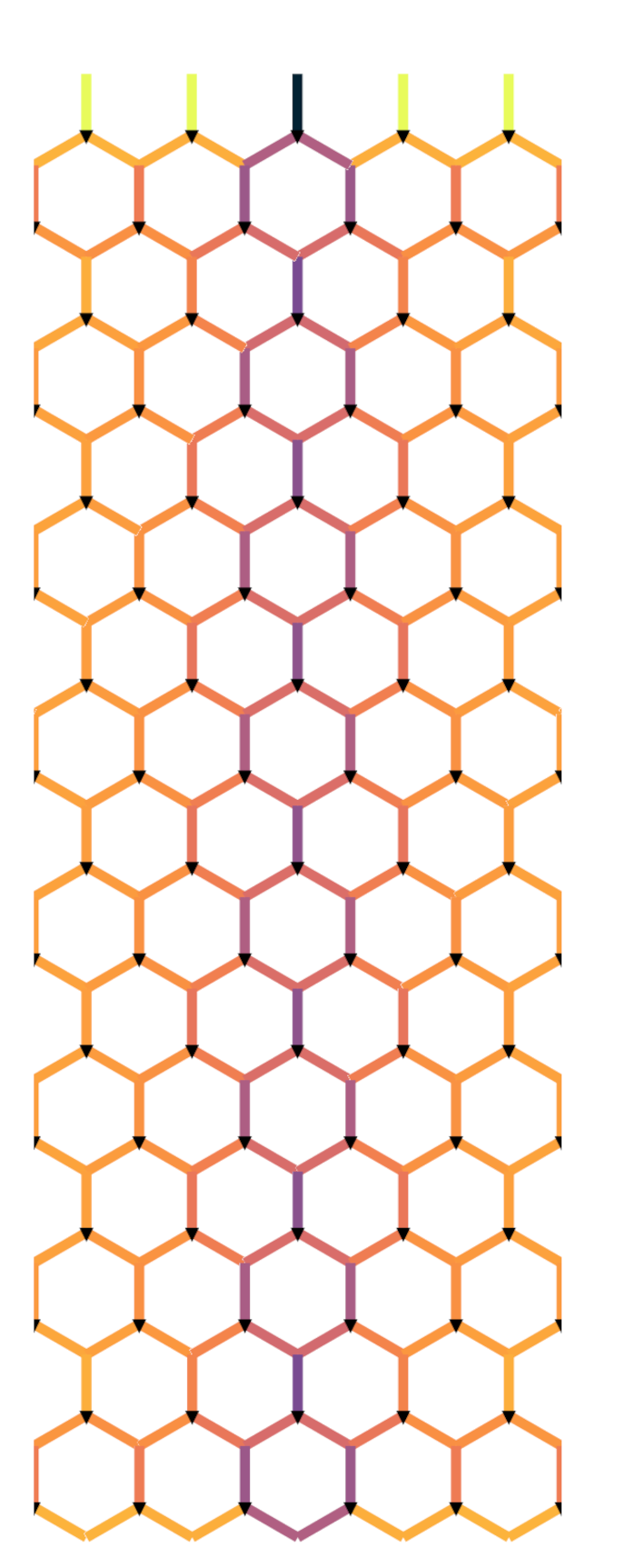
The ground state is calculated for $N_{x}\times N_{y}$ systems (see fig. 2) with $N_{x}\in\{3,4,5\}$, periodic boundary conditions in the $x$-direction and closed boundary conditions in the $y$-direction, both with and without an unbreakable flux string in the $y$-direction. An example of this geometry can be seen in fig. 2 together with an example of a flux string in fig. 3. This was done for $N_{y}\in\{2,4,\dots,14,16\}$ and $g^{2}\in\{0.5,0.75,\dots,7.75,8\}$. For a fixed system size, first the vacuum state, in case of the systems without $\frac{1}{2}$ charges on the edges, or otherwise a superposition of the vacuum with the shortest path string is used as an initial state for $g^{2}=8$ which is fairly close to the true ground state Kogut (1979). The resulting ground state is then used as the initial state for the DMRG at the next smallest $g^{2}$. For $g^{2}=8$, the minimum sweeps are set to $50$ with $15$ noise sweeps to ensure that the correct ground state is found. For all further calculations the minimum sweeps are $7$ with $4$ of them noisy. To prevent the MPS from exceeding the available RAM, a maximum bond dimension of $2000$ is imposed. However, based on the calculated truncation error, this does not seem to significantly affect the results. For the resulting states, the energy, the variance of the Hamiltonian, the expectation values of the penalty terms and the expectation values of the projectors onto each of the four even site basis states on each link are saved. Furthermore, for the chargeless systems only, the electric part of the energy is measured separately.

Figure 2: Exemplary plot of the simulated geometry for $N_{x}=5$ and $N_{y}=8$. The black triangles indicate the even site basis sites and the black arrow signifies the way in which the $1$d MPS is inlaied into the $2$d system.

Figure 3: Exemplary plot of a flux string ground state at $g^{2}=1.5$. For each link, the expectation value of $\mathbb{1}-\ket{0}\bra{0}$ is plotted signifiying the total flux carried by the link. Dark blue is $1$, yellow is $0$.

III.2 Convergence

Since DMRG can get trapped in local minima, it is vital to check that convergence was achieved. For large systems the convergence to the true global minimum is difficult to quantify. Here an approximation is used that states that for states that are close to the ground state

$$\frac{\text{Var}(H)}{(\Delta m)^{2}}=(1-f)+\mathcal{O}\left((1-f)^{2}\right)$$ (15)

holds where the variance is computed with respect to the DMRG output, $\Delta m$ is the mass gap of the system and $f=|\braket{\Psi_{\text{exact}}|\Psi_{\text{approx}}}|^{2}$ is the fidelity. Since the true mass gap is unknown it is substituted by the mass gap of the $4\times 4$ lattice of the same topology obtained via exact diagonalization for all couplings. It should be noted that the mass gap tends to slightly decrease as the volume increases, however by comparison to previous mass gap calculations Engels and Mitrjushkin (1992) it can be estimated that for the ratios of volumes required $(\Delta m)^{2}$ is at most overestimated by a factor of $10$. As can be seen in fig. 4 the approximated infidelity is for many cases around or below $10^{-4}$ with some larger systems with strings around $10^{-3}$ indicating a good convergence for all systems. The infidelities both of larger systems and of systems containing strings are generally larger.

Figure 4: $\text{Var}(H)/(\Delta m)^{2}\approx(1-f)$ for the empty systems (top) and the systems with strings (bottom).

As a side it should be noted that for the runtime of the DMRG two different behaviours were observed as plotted in fig. 5. For systems without a string the runtime increased linearly starting from $N_{y}=6$ as would be expected of a system with a small correlation length. For the systems with a string the runtime increased as a higher order polynomial. It seems likely that this higher order polynomial is the effect of a large increase in the correlation length induced by the strings.

Figure 5: Total runtime for each coupling both with and without a string in a log-log plot for $N_{x}=5$.

IV Results

Using the methods described in the previous sections we have investigated the QLM on the hexagonal lattice in a wide range of bare couplings $0.5\leq g^{2}\leq 8$, with 8 additional points at $95\leq g^{2}\leq 125$. Moreover, we study the dependence on the transversal lattice extent $N_{x}$ with values $N_{x}=3,4$ and $N_{x}=5$.

IV.1 Electric versus Magnetic Contributions to $H$

It is well known that the Kogut-Susskind Hamiltonian exhibits a magnetic regime at small $g^{2}$ where $H_{M}$ dominates and an electric regime at large $g^{2}$ where $H_{E}$ dominates. In this model they can be distinguished via the average fraction of flux transporting links

$$\bar{\nu}\ =\ \frac{1}{|\Lambda|}\sum_{i\in\Lambda}\langle 1-\ket{0}\bra{0}\rangle_{i}$$ (16)

shown in fig. 6. Here $\Lambda$ is the set of all links in the lattice. In the electric regime ($g^{2}\to\infty$) this value goes to zero while it attains a finite value in the magnetic regime, as can be seen in fig. 6 where we show $\bar{\nu}$ as a function of $g^{2}$ for different $N_{y}$. Given the quick convergence to a universal curve for large $N_{y}$ visible in fig. 6, it seems likely that there is no phase transition but a crossover between the two regimes.

Figure 6: Fraction of flux transporting links $\bar{\nu}$ as a function of the coupling $g^{2}$ for different $N_{y}$ at $N_{x}$=5

Fitting this data with a generalized logistic function

$$\bar{\nu}(g^{2})=b(1+\exp(d(g^{2}-c)))^{-m}$$ (17)

for each system length $N_{y}$, we can then exponentially extrapolate $b$ (shown in fig. 7) and $c$ (shown in fig. 8) in $N_{y}$ using the ansatz

$$y=-\alpha\ \text{exp}(-\beta N_{y})+\gamma\,.$$ (18)

Excluding $N_{y}=2$ from the fits, we obtain the fraction at $g=0$ as $\bar{\nu}_{g=0}=0.227(1)$ and the crossover point at $g^{2}=3.09(4)$ in the limit $N_{y}\to\infty$.

Figure 7: Infinite length extrapolation for the fraction of flux carrying links at $g^{2}=0$ with $\chi^{2}_{\text{red}}=0.03$ and $N_{x}=5$. The data point at $N_{y}=2$ is excluded from the fit. The parameters are $\alpha=-0.06(6)$, $\beta=0.5(3)$ and $\gamma=0.227(1)$

Figure 8: Infinite length extrapolation for the center of the crossover with $\chi^{2}_{\text{red}}=0.006$ and $N_{x}=5$. The data point at $N_{y}=2$ is excluded from the fit. The parameters are $\alpha=1(2)$, $\beta=0.5(5)$ and $\gamma=3.09(4)$

IV.2 The static quark potential

By subtracting the ground state energy of the system without charges of the same size from the ground state energy of a system containing a charge pair, one can compute the static quark potential $V(r)$ eq. 14 for this theory. Since the charges are located at the upper and lower boundaries, respectively, the potential $V$ is evaluated at distance $r=N_{y}$, and we vary $N_{y}$ to probe different distances. The data for small $N_{y}$ is excluded from the fits as it contains large finite size and discretization effects. For $N_{x}=5$ only $N_{y}\geq 6$, for $N_{x}=4$ only $N_{y}\geq 10$ and for $N_{x}=3$ only $N_{y}\geq 8$ are used. The amount of the effect as well as the system lengths at which it occurs seems to depend both on the width of the system and on the parity of the systems width and length. We observe a positive string tension $\sigma$ for all values of $g^{2}$ investigated, indicating confinement. At least visually, there are barely deviations from the linear dependence on $r$ visible. This is shown exemplarily in fig. 9, where we show the potential in lattice units as a function of $N_{y}\equiv\frac{2r}{3}$ for $g^{2}=4$. Note that the factor $2/3$ in the relation between $r$ and $N_{y}$ stems from the hexagonal geometry in the investigated lattice.

Figure 9: Potential $V$ as a function of $N_{y}$ for transversal lattice extent $N_{x}=5$ and $g^{2}=4$. The dashed (red) line represents a fit of eq. 14 to the data for $N_{y}>4$.

In fig. 10 we show the string tension $\sigma$ as a function of $g^{2}$. The string tension measured in the simulations is in so-called lattice units, i.e. $\sigma=a(g)^{2}\sigma_{\mathrm{physical}}$, where $\sigma_{\mathrm{physical}}$ has units of energy squared. The value of $\sigma_{\mathrm{physical}}$ is not know, because there is no realization of this QLM in nature, but its value in physical units is also not needed. If this universal curve exists, one can use $\sqrt{\sigma}=a\sqrt{\sigma_{\mathrm{physical}}}$ and its inverse to quote distances and energies in units of (inverse) $\sqrt{\sigma}$. If this theory indeed exhibits a universal observable $\sigma_{\mathrm{physical}}$, $V(r\sqrt{\sigma})/\sqrt{\sigma}$ will be a universal curve, up to discretization artifacts. This is the case as can be observed in fig. 11, with basically no lattice artifacts visible.

Figure 10: String tension $\sigma$ as a function of $g^{2}$ with $N_{x}=3$ (blue diamond), $N_{x}=4$ (red dot), and $N_{x}=5$ (black x).

Figure 11: Static potential in units of $1/\sqrt{\sigma}$ as a function of the distance $N_{y}\sqrt{\sigma}$ including data for all values of $g^{2}$. The different colors represent data points with $N_{x}=3$ (blue diamond), $N_{x}=4$ (red dot), and $N_{x}=5$ (black x).

The string tension, therefore, gives also access to the lattice spacing: from fig. 10 it can be read off that for this model the lattice spacing diverges both for strong and weak coupling. For $g^{2}=100$ the string tension was additionally determined to be $\sigma=299.79950(4)$ which is consistent with a linear increase of the string tension for large coupling. We remark that we have performed the equivalent procedure using the so-called Sommer parameter Sommer (1994) with the results being in good agreement with the ones from the string tension. We also remark that in $2+1$ dimensions the coupling is dimensionful, i.e.

$$g^{2}=ag_{0}^{2}$$ (19)

with $g_{0}$ the bare running coupling of the theory. However, if one used $1/a$ as the energy scale at which to define $g_{0}$, the bare coupling $g_{0}(1/a)$ is not uniquely defined.

When fitting to the data of the potential $V(N_{y})$, we also include a term proportional to $\gamma/N_{y}$ corresponding to the Lüscher term with $\gamma$ as a fit parameter. Indeed, the inclusion of this term in the fit improves the $\chi^{2}/\mathrm{dof}$ significantly. The $1/r$ term indeed describes the data excellently, which can be see in fig. 12 where we plot $V(N_{y})-\sigma N_{y}$ - c as a function of $N_{y}$. The dashed line is the fitted curve, the shapes represent the data points. Note that the relative contribution of the Lüscher term is still only around $0.1\%$ for large $g^{2}$ and $0.5\%$ for small $g^{2}$, which is why the $1/r$ term is invisible in fig. 9.

Figure 12: Lüscher term contribution of the potential for different $g^{2}$ in units of the string tension for the lattice widths $N_{x}$ of $5$ (top), $4$ (middle), and $3$ (bottom). $V_{\text{luescher}}=V(N_{y})-\sigma N_{y}-c$.

The results for the Lüscher term ($\gamma$ in eq. 14) are plotted in fig. 13 as a function of $g^{2}$. For $g^{2}<2$ the value of $\gamma$ trends towards large negative values. For large $g^{2}$-values, on the other hand the measured $\gamma$-values tends towards zero. While the measured value of $\gamma$ is at $g^{2}=8$ still a factor of about eight larger in modulus than the expected $-\pi/24$, the modulus is smaller than $\pi/24$ at $g^{2}=95$, see the lower panel. Therefore, there is a $g^{2}$-value between $8$ and $95$ where $\gamma=-\pi/24$. Moreover, the observed value fo $\gamma$ appears to approach zero slowly for $g^{2}\to\infty$. At $g^{2}=\infty$, $\gamma$ must equal zero as the magnetic part in the Hamiltonian becomes irrelevant.

In the upper panel of fig. 13 we show the best fit value for $\gamma$ for three different transversal widths $N_{x}$ of the lattice. At large values of $g^{2}$, we observe a mild dependence on $N_{x}$, see the inlet in the figure. However, there appears to be no monotonous convergence in $N_{x}$. $N_{x}=4$ results lie in between the $N_{x}=5$ and $N_{x}=3$ results only for a small intermediate region of about $3<g^{2}<4.5$. For small values of $g^{2}$, finite size effects quickly become larger than $100\%$.

Finally, for the largest $N_{x}$-value, we observe a fish bone structure in the $g^{2}$-value region between $4$ and $7$. This is a hysteresis-like effect introduced by the DMRG on MPS algorithm used, which utilizes the converged state of the next largest $g^{2}$ as the initial state for every new value of $g^{2}$. It is usually too small to be relevant but can be seen here due to the relatively small contribution of the Lüscher term in this model that makes it more sensitive to such effects. The effect is short-lived in the sense that, once a sufficient accumulation of error has taken place, the DMRG algorithm will converge back to the correct state.

Figure 13: Best fit value of $\gamma$ as a function of $g^{2}$ for three different width of the lattice $N_{x}=3$ (blue diamonds), $N_{x}=4$ (red dots) and $N_{x}=5$ (black crosses). Additional data points for $N_{x}=5$ at large coupling are added to confirm the scaling behavior for the large coupling limit.

IV.3 String width $\omega^{2}$

Figure 14: Exemplary plot of the transversal cut used to obtain the flux profile for $N_{y}=4$ (right) and $N_{y}=6$ (left) at $N_{x}=5$

As mentioned before, one property of rough strings is the logarithmic scaling of its (squared) width $\omega^{2}$ with the length $r$. $\omega^{2}$ can be extracted from the flux distribution of the cross-section of the strings. For this we perform a cut through the lattice in the transversal direction as close to the longitudinal centre of the string as possible while maximising the number of cut links at the same time. These criteria result in a cut slightly above (below) the centre of the string, as visualised in fig. 14. The effect of this slight deviation from the longitudinal centre will become negligible quickly with increasing string length. Plotting the flux as a function of the distance from the transversal centre as exemplarily shown in fig. 15, reveals a Gaussian-like distribution with heavy tails which is well-fitted by a Gaussian with smooth exponential Verzichelli et al. (2025) tails given by

$$\begin{split}f(x)=\begin{cases}A\,\text{exp}\left({-\dfrac{x^{2}}{2\omega^{2}}}\right)+c&|x|\leq x_{0}\\ A\,\text{exp}\left({-\dfrac{x_{0}^{2}}{2\omega^{2}}-\dfrac{x_{0}}{\omega^{2}}\left(|x|-x_{0}\right)}\right)+c&|x|>x_{0}\end{cases}.\end{split}$$ (20)

Here, $x_{0}$ represents the distance from the centre of the string from which on the heavy tails are added to the functional form. Thus, $f(x)$ from eq. 20 depends on three fit parameters, $A,\omega^{2}$ and $x_{0}$. Two exemplary fits with different couplings $g^{2}=0.5$ and $g^{2}=8$ and string length $N_{y}=12$ are displayed in fig. 15.

Figure 15: Flux distribution of $p=\langle\mathbb{1}-\ket{0}\bra{0}\rangle$ on each link centrally wrapped around the system over the orthogonal distance from the string centre $x$ for $g^{2}=8$ (top) and $g^{2}=0.5$ (bottom) with $N_{y}=12$, fitted with eq. 20. $x_{0}$ is plotted as gray dashed lines.

By performing such fits for all couplings and lengths of the strings at the largest $N_{y}$ of $5$, the scaling of the width $\omega^{2}$ with the length of the string can be extracted. The results for $\omega^{2}$ are plotted for select $g^{2}$ values in fig. 16 as a function of $N_{y}\propto r$.

Figure 16: String widths $\omega^{2}$ over $N_{y}$ for selected $g^{2}$ and $N_{x}=5$. The solid line represent fits to the data with logarithmic functional form eq. 21 including all points with $N_{y}\geq 6$ (see text) in the fit.

In general, the width increases with $N_{y}$. The observed zigzag behaviour overlaying this increase originates again from the geometry of the lattice: For $N_{y}$ divisible by $4$ the shortest path for the string is via one single link in the longitudinal centre, while for the other $N_{y}$ values there are two shortest paths with equal length. This can be nicely seen in fig. 14. Since this is not only the case at the centre of the string, this effect becomes less and less relevant towards larger $N_{y}$ values. In order to reduce the influence of this zig-zag modulation, in the following we only consider $N_{y}\geq 6$.

For a rough string, which ordinarily possesses a Lüscher term, one would expect a logarithmic scaling of the width in the length of the string. For rigid strings, on the other hand, the width is expected to be constant as the length is increased. Clearly, our results for $\omega^{2}$ are not well described by a constant, which is why we attempt a fit of the form

$$\omega^{2}(N_{y})=A\ \text{ln}(N_{y}-b)$$ (21)

to the data. As can be seen in fig. 16 for $N_{y}\geq 6$ all data points are well described by the fit.

V Discussion

The SU$(2)$ QLM investigated in this paper clearly exhibits confinement for all values of $g^{2}$ investigated. While this is expected for this model, it appears remarkable to us how well the data for the static potential fall on a universal curve once plotted in appropriate units, cf. fig. 11. At least visually there are no deviations from the linear behaviour observable up to value of $N_{y}\sqrt{\sigma}>150$.

The results for the Lüscher term and the width of the string deserve further discussion here. First, the results for the Lüscher term presented above are inconclusive. One major reason for this is the fact that we could only study transversal extensions of the lattice up to $N_{x}=5$. The finite size effects we observe in $\gamma$ when comparing $N_{x}=3,4,5$ indicate that certainly in the region of small $g^{2}$-values $N_{x}=5$ is not sufficient to be conclusive: finite size effects could still be of the order of $100\%$. At large $g^{2}$-values, the dependence on $N_{x}$ is much milder, however, convergence is not monotonous in $N_{x}$. Clearly, in the future larger values of $N_{x}$ need to be studied to clarify this point.

Strong finite size effects on the Lüscher term were also observed in Ref. Di Marcantonio et al. (2025) in a $\mathbb{Z}_{2}$ Abelian gauge theory. However, it should be mentioned that $N_{x}=5$ must be multiplied by $\sqrt{3}\approx 1.7$ in comparison to Ref. Di Marcantonio et al. (2025), and is thus in principle larger than the maximal transversal extent of $6$ in lattice units used in that reference, despite the fundamentally different theories.

Another point to highlight is that the error estimate for $\gamma$ is not statistical but comes from the $\chi^{2}$ fit only. It is unclear to us whether our error estimates are accurate such that the uncertainties in fig. 13 should be taken with care.

The obvious question of why a Lüscher-like term is observed, but with a value for $\gamma$, which agrees to the universally expected value only at a single $g^{2}$-value between $g^{2}=8$ and $g^{2}=95$. In our opinion there are two possibilities: one is that significantly larger volumes are required to see convergence to the universal $\gamma$-value in some $g^{2}$ interval. Another other possibility could b that lattice artifacts induce a modification to the $1/r$ term in the potential, for instance of the form $\gamma(1+a\,X)$, where $X$ would be dimensionful and proportional to some operator expectation value. Of course, it is actually unlikely that such an expansion à la Symanzik Symanzik (1983) exists in the model at hand. Since the values of the string tension indicate that in this QLM the lattice spacing is at no value of $g^{2}$ small, it could mean that the values of $\gamma$ we observe are dominated by lattice artefacts entirely. Unfortunately, the latter hypothesis is not testable, because we cannot take a continuum limit.
As both of these possibilities are not very credible, $\gamma$ might have this observed $g^{2}$ dependence in this QLM, and it would remain to understand why the effective string theory is not applicable.

The Lüscher term has been studied previously using stochastic Monte Carlo simulations in the Lagrangian formulation Bali et al. (1995); Lüscher and Weisz (2002) in particular also in SU$(2)$ Caselle et al. (2004); Hari Dass and Majumdar (2008); Pepe and Wiese (2009). In comparison, the major advantage of the Hamiltonian formalism is the absence of statistical uncertainties, which grow in stochastic simulations towards larger distances such that the signal-to-noise ratio deteriorates exponentially, a problem which can be only solved in principle by multi-level approaches Lüscher and Weisz (2002); Barca et al. (2024). However, the results presented in this paper show that with the current volumes feasible in TNS simulations this advantage does not play out as yet.

The width of the string, on the other hand, appears to scale logarithmically with the length of the string for all values of the coupling investigated here. While a linear dependence on the length of the string is not excluded, it is certainly not independent of the length of the string as expected for a rigid string. We interpret this result as an indication for a rough string for all values of the coupling investigated here. This includes in particular also the values of the coupling where the electric part in the Hamiltonian dominates the dynamics, which is surprising to us: we would expect a rigid string for large values of $g^{2}$ as observed in other SU$(2)$ gauge theories, and correspondingly a roughening transition. However, if this roughening transition existed in this QLM, it would need to be for values of $g^{2}$ larger than $125$.

VI Conclusion & Outlook

In this paper we have investigated a $(2+1)$-dimensional non-Ablian SU$(2)$ quantum link model using the $5$-dimensional representation of the embedding group SO$(5)$. We have simulated this theory with exact non-Abelian SU$(2)$ local gauge symmetry for the first time using matrix product state algorithms on a hexagonal lattice, which can be mapped particularly efficiently to the MPS.

We have computed the static potential as a function of the distance by studying configurations with and without two separated static charges. The first remarkable result is that the string tension $\sigma$ can be extracted for all values of the coupling to be positive, indicating a confined theory for all values of the bare coupling. Using again the string tension, we have then shown that there exists a unique potential in units of $\sqrt{\sigma}$ for all values of the bare coupling. However, the lattice spacing does not approach zero with $g^{2}\to 0$, but increases again for $g^{2}<4.687(2)$. Thus, as expected, a continuum limit does not exist for this QLM in the traditional sense.

Moreover, we have investigated the so-called Lüscher term, a $\gamma/r$ contribution to the potential at large distances, with $\gamma=-\pi/24$ known from effective string theory in $2+1$ dimensions. Our results for the Lüscher term are inconclusive, with measured values for $\gamma$ all negative, but modulus from close to zero at $g^{2}=100$ to larger than $20$ for $g^{2}=0.5$. We have discussed finite size effects or lattice artefacts as possible reason for this finding, even though they are unlikely to fully explain our findings.

Even if with the simulation volumes currently feasible in TN simulations the Hamiltonian formalism are not yet competitive with Monte Carlo, we expect that in the not too distant future it will be possible to determine even subleading contributions to the potential in the Hamiltonian formalism. This is mainly due to the absence of statistical uncertainties, which on the other hand make it even more important to control all the systematics.

Finally, the investigation of the width of the string as a function of the string length indicates that the strings are rough again for all values of the bare coupling. This conclusion is supported by the squared string width increasing like the logarithm of the length of the string in the whole range of $g^{2}$-values we investigated. This means also that we could not identify a roughening transition up to $g^{2}=125$.

In the future larger transversal lattice extents or in general larger volumes must be investigated in order to better control the associated finite-size effects. For the same reason also other systematic effects of the method need to be thoroughly studied in order to fully profit from the advantages of the Hamiltonian formalism. Moreover, it might be needed to check whether or not the assumption that universal value $-\gamma=\pi/24$ is unaffected by the hexagonal geometry of the lattice holds, or whether the effective string theory is not applicable for some other reason. Moreover, if $\gamma$ approaches zero smoothly, i.e. without a phase transition, the strong coupling expansion of the model could be investigated to gain further insights.

Finally, given the results presented in this paper, it appears promising and highly interesting to also investigate larger representations of SO$(5)$ in order to understand QLMs better in general, and to eventually prepare for simulations on quantum devices.