Abstract

We propose an efficient retraining strategy for a parameterized Reduced Order Model (ROM) that attains accuracy comparable to full retraining while requiring only a fraction of the computational time (from 2 hours to $\approx 15$ minutes) and relying solely on sparse observations of the full system of order $10^{1}$ to $10^{2}$. The architecture employs an encode–process–decode structure: a Variational Autoencoder (VAE) to perform dimensionality reduction, and a transformer network to evolve the latent states and model the dynamics. The ROM is parameterized by an external control variable, the Reynolds number in the Navier–Stokes setting, with the transformer exploiting attention mechanisms to capture both temporal dependencies and parameter effects. The probabilistic VAE enables stochastic sampling of trajectory ensembles, providing predictive means and uncertainty quantification through the first two moments. After initial training on a limited set of dynamical regimes, the model is adapted to out-of-sample parameter regions using only sparse data. Its probabilistic formulation naturally supports ensemble generation, which we employ within an ensemble Kalman filtering framework to assimilate data and reconstruct full-state trajectories from minimal observations. We further show that, for the dynamical system considered, the dominant source of error in out-of-sample forecasts stems from distortions of the latent manifold rather than changes in the latent dynamics. Consequently, retraining can be limited to the autoencoder, allowing for a lightweight, computationally efficient, real-time adaptation procedure with very sparse fine-tuning data.

newfloatplacementnewfloatnamenewfloatfileextnewfloatwithin

1 Introduction

Modelling physical systems using data-driven approaches remains a notoriously difficult task. Even for seemingly simple systems, the challenge arises due to (i) their nonlinear behaviour, high dimensionality, and complex space–time dependencies, and (ii) the fact that the available data are often sparse, noisy, and expensive to generate [Kelshaw_Magri].

To address the first challenge, Reduced-Order Models (ROMs) are a powerful framework capable of transforming limited data into meaningful predictions by exploiting latent low-dimensional structures within the system, essentially mining simplicity from complexity. These low-dimensional structures, commonly referred to as manifolds, can be defined in several ways. They may exist in a space spanned by physical observables, as in a phase space [SSM-1, SSM-2], or in a basis of modes derived from a linear projection onto a low-dimensional latent space that maximizes energy [POD_Schmid]. Alternatively, they can be identified in a purely data-driven manner by minimizing reconstruction error, as in nonlinear autoencoders, resulting in a highly compressed and abstract latent space. Remarkably, such low-dimensional manifolds can exist in chaotic systems [ChaoticSSM]. Once identified, the system dynamics can be projected, simplified. Methods to achieve this can be either intrusive [CD-ROM, ql-ROM] or non-intrusive [ILED, Gupta, VpROM], i.e., data-driven.

Statistical mechanics have long emphasized the importance of memory, which effect plays a central role in recovering partial system states. This insight has repelled dynamical models from the attractor of Markovian determinism, which even finite Koopman subspaces often fail to represent accurately. The Mori-Zwanzig formalism and Takens’ theorem [Taken, Mori, Zwanzig] emphasize the importance of incorporating a memory term to effectively account for the influence of the unobserved, orthogonal subspace on the set of observables learned or selected during the reduction. Additionally, studies aiming at uncovering finite Koopman spaces [Gupta] demonstrate the limitations of using a purely Markovian representation for rolling out dynamics within a finite, invariant Koopman space. The concept now has further influenced data-driven modelling. Notable examples include reservoir computing [Real_time_calibration_chaotic, racca_2023], embedded memory [Gupta] and, most recently, attention mechanisms and transformers [Attention]. These developments have substantially reshaped the landscape of nonlinear dynamical modelling [SLT, AutoencoderTransformer, UPdROM].

Identifying suitable latent manifolds, however, remains nontrivial. An ill-defined manifold leads to error propagation from the latent dynamics to the system’s physical states, causing predictions to diverge from the true trajectories even after moderately long rollouts [thermalizer]. Correcting this divergence, either in real time through control or a posteriori through fine-tuning, may therefore be necessary. However, both strategies typically require additional data, giving rise to a data bottleneck when incorporating a posteriori knowledge of the true system state into the model’s predictive process.

Most existing approaches assume access to high-fidelity, fully sampled simulation or experimental data for training and fine-tuning, an assumption that rarely holds in practice. During fine-tuning, we instead assume that the model’s prediction of the high-dimensional state is only partially correct. This partial correctness can be exploited in conjunction with sparse high-fidelity measurements, for instance, those obtained from physical sensors, to enhance model accuracy and robustness. The problem can also be viewed through a statistical lens, where the new, limited fine-tuning data are combined with imperfect prior estimates whose error covariances are explicitly accounted for. In this framework, inaccurate model predictions are not discarded but treated as uncertain observations, allowing their associated uncertainty to guide the integration of sparse, high-fidelity data. This principle underpins Kalman filtering, where an error-prone model estimate is combined with limited yet accurate observations and has been applied extensively in the data-assimilation community [DA, bocquet_2]. When this condition holds, Kalman filters can be applied effectively across a broad range of contexts, including real-time control [Real_time_calibration_chaotic], reinforcement learning [Control_turbulence_DA], and a posteriori model retraining [bocquet_2].

Kalman filters are purely statistical in nature and do not depend on the physical properties of the underlying system. Consequently, they have been successfully employed in complex parametric spaces [parameter_augmented_DA] and in turbulent flow applications [turbulence_DA, Eldredge_1, Zaki].

Our approach is inspired by that of [bocquet_2] in that the model is retrained a posteriori using fine-tuning data generated through Kalman-filter–based data assimilation. The dynamical model used in this work is a stochastic Reduced-Order Model (ROM), described in Section 3, and builds upon previous developments that did not incorporate sparse-data constraints [UPdROM]. The stochastic nature of the ROM provides ensembles of predictions, whose variance is used as a proxy for model error. A central focus of this work is to alleviate the cost associated with generating fine-tuning data. To this end, the methodology leverages ensemble predictions within a Gaussian-based uncertainty-quantification framework. This inherent Gaussianity enables efficient reconstruction of full-state information from sparse, high-fidelity measurements distributed across the physical domain via Kalman filtering. The model, originally trained in a specific region of the testing distribution, is subsequently fine-tuned in a different region using only a minimal amount of additional data. What distinguishes our method is the tight integration of probabilistic ROMs with Kalman filtering, specifically tailored for parametric dynamical systems. This integration allows the model to adapt across different parameter regimes, each characterized by distinct system behaviours, whereas traditional approaches would require costly, full-state, high-fidelity data to achieve comparable adaptability.

The paper is structured as follows. Section 2 introduces the experimental setup and the ROM used in this study. Section 4 then investigates the training of the ROM, together with an analysis of the resulting latent space and manifold, and their impact on learning performance. This analysis reveals a remarkable economy in training requirements, as only the projection onto the latent space requires fine-tuning. Finally, this economy is exploited in Section 5, where sparse observations and Kalman filtering are combined to efficiently retrain the model. Conclusions and perspective of the work are presented in Section 7.

2 Parametrised dynamical system

We consider the following equation, which describes a general form of a dynamical system:

$$\frac{d\psi}{dt}=F(\psi,\xi,t),$$ (1)

where $F$ is a nonlinear operator governing the spatial and temporal evolution of the system. Here, $\psi$ denotes the state variables, and $\xi$ represents the parameters influencing the system’s dynamical behaviour. In this study, the dynamical system is represented by an unsteady, two-dimensional flow past an obstacle. Given this representation, the above equation can be recast as the incompressible Navier–Stokes equations, which are given below:

$$\frac{\partial\mathbf{\psi}}{\partial t} =-\nabla p-(\mathbf{\psi}\cdot\nabla)\mathbf{\psi}+\frac{1}{Re}\nabla^{2}\mathbf{\psi},$$ (2)

$$\nabla\cdot\mathbf{\psi} =0.$$

Here, $\psi$ is the velocity field $[u,v]^{T}$ and $p$ the pressure field. The flow behaviour is primarily influenced by the Reynolds number $Re=\frac{\rho UL}{\mu}$, where $\rho$ is the fluid density, $U$ is the characteristic velocity, $L$ is the characteristic length (such as the length of the bluff body), and $\mu$ is the dynamic viscosity of the fluid. This quantity is treated here as the variable model parameter $\xi$. Even varying the Reynolds number across a moderate range provokes a qualitatively different dynamical response from the system. Increasing the Reynolds number can cause the system to bifurcate, resulting in sharper transitions to the onset of instabilities or different periodic orbits. Previous work have studied the system’s behavioural dependency to the Reynolds number in the case of a cylinder. Experimental and numerical results exhibit an initial bifurcation at $Re\sim 48$ followed by an instability growth rate linearly dependant to the Reynolds number [Canuto_Taira_2015, Strykowski_Sreenivasan_1990]. In our experimental set-up, the ”Hopf” bifurcation occurs at $Re\sim 60$. This is because the obstacle is an ellipsoid with an aspect ratio greater than one, thereby resembling a symmetric airfoil profile. This configuration offers the advantage of exhibiting a dynamical behavior characterized by a single periodic orbit over a broader range of Reynolds numbers than with a cylinder for instance. It can be visualized in Figure 1 along the energetic behaviour of our system prior and posterior the bifurcation.

Figure 1: Hopf bifurcations with latent manifolds at $Re=50$ and $Re=90$. $U$ velocity field at unstable fixed point and at limit cycle.

We are interested in the regime at moderate Reynolds numbers, within the range $Re\in[80,140]$. The model may struggle to generalize and extrapolate effectively across this range, particularly near the upper boundary, thus necessitating fine-tuning. Thus, the flow regime considered here lies beyond the onset of instability and is characterized by the emergence of a single periodic orbit. The system is initialized at the unstable fixed point, which exhibits nearly stationary behaviour before transitioning to its stable limit cycle. In this test case, the limit cycle corresponds to the well-known Von Kármán vortex street forming in the wake of the obstacle. This transition is illustrated in Figure 1. The system state is discretized on an Eulerian grid of size $131\times 100$, resulting in a high-dimensional state space of 13100 variables for the two velocity components $u$ and $v$. We use an Immersed Boundary Method solver (ibmos) [IBMOS] to generate training data.

To address the complexity inherent to the high dimensionality of our problem, we train a parameter-dependent Reduced Order Model (ROM) that exploits the low-dimensional nature of the manifold on which the system’s dynamics evolve.

3 Parametric Reduced Order Model (ROM)

Dynamical systems often converge towards low-dimensional structures, known as manifolds, on which the system’s dynamics evolve. To effectively represent the system’s state and evolve it in time, we have developed a model that compresses the spatial information while simultaneously modeling the temporal dependencies within this reduced-dimensional manifold [UPdROM].

We employ a Variational Autoencoder (VAE) [VAE] to identify a reduced latent space onto which the dynamics are learned by a Transformer, leveraging recent advances in embedded memory and attention mechanisms [Attention, SLT].

Figure 2: Our Reduced-Order Model encodes and reduces with $\mathcal{E}$ both velocity fields $U$ and $V$ along with the parametrisation $\xi$. The transformer rolls-out the dynamics auto-regressively in the latent space with self-attention and cross-attention with $\xi$. Finally the decoder $\mathcal{D}$ projects the latent states and $\xi$ back to the physical space.

Our architecture, illustrated in Figure 2, is based on the design proposed in UP-dROM: Uncertainty-Aware and Parametrised dynamic Reduced-Order Model [UPdROM]. The model learns unsteady-state behaviour and performs dynamical rollouts from initial conditions in an auto-regressive fashion. We leverage cross-attention in the latent space to account for the parametric dependence allowing the model to capture intricate and nonlinear space-time relationships, including interactions with external variables such as the Reynolds number. The Encoder–Decoder is explicitly conditioned on the Reynolds number since different regimes may correspond to distinct regions of the latent manifold [ql-ROM]. The theoretical foundations and implementation details of that ROM are publicly available on GitHub [GitHubRepo] and in UP-dROM paper.

A notable aspect of our approach is the use of a Variational Autoencoder (VAE). Beyond producing a well-structured and dense latent space that improves generalization, the VAE learns a distribution over latent variables, enabling the generation of diverse yet physically plausible trajectories. This probabilistic framework naturally supports stochastic sampling and uncertainty quantification, as demonstrated in UP-dROM, and also allows for ensemble generation, whose probabilistic moments can be leveraged in a Data Assimilation frameworks.

For training, the original $131\times 100$ grid is flattened to a $13{,}100$-dimensional vector and downsampled by a factor of 4, yielding $3{,}275$ degrees of freedom. Since both velocity components $(u,v)$ are modeled simultaneously, the resulting input space lies in $\mathbb{R}^{6{,}550}$. The VAE then learns a mapping $\mathcal{E}$

$$\mathcal{E}:\mathbb{R}^{6{,}550}\rightarrow\mathbb{R}^{4},$$

with the Transformer trained jointly on the latent representations. Additional details on the architecture and hyperparameters are provided in  A.1.

3.1 Model performance across the parametric region

We initially train the model only at $Re=90$ and $Re=120$. The seven inference cases are at $Re\in\{80,90,\dots,130,140\}$, thereby covering both interpolation and extrapolation regimes. The dataset consists of $T=3033$ snapshots, with an input dimension of $m=6550$. We split the dataset into training and testing sets by assigning even snapshots to the training set and odd snapshots to the test set to ensure equal share of transients and limit cycle to both datasets. Accordingly, the training set has dimensions $\mathbb{R}^{2,T/2,m}$, and the test set also has dimensions $\mathbb{R}^{2,T/2,m}$. Finally, the validation set has dimensions $\mathbb{R}^{7,T/2,m}$, containing system states for all considered Reynolds numbers. The validation set is designed to explore the parameter space, enabling an assessment of the model’s generalization performance, even though the model was trained only in a sub-region of this space. In the parameter space of interest, the dynamics exhibit different characteristics. Specifically, there is an instability that evolves towards an attractor, that varies in geometry and magnitude when the parameters change.

Kinetic energy is used to evaluate the performance of the model. It aggregates both velocity components $(u,v)$ into a single physically meaningful quantity, and for a given parameter $\xi$ is computed as:

$$k_{\xi}=u_{\xi}^{2}+v_{\xi}^{2},\quad k_{\xi}\in\mathbb{R}^{T/2,D}.$$ (3)

Model performance is assessed in forecast mode on the test set using the 2-Wasserstein distance, also known as the energy distance. This approach treats the predicted and true trajectories as probability distributions. The 2-Wasserstein distance between two probability measures $P$ and $Q$ on $\mathbb{R}^{d}$ [Wasserstein_dist] is defined as

$$W_{2}(P,Q)=\left(\inf_{\pi\in\Gamma(P,Q)}\int_{\mathbb{R}^{d}\times\mathbb{R}^{d}}\|x-y\|^{2}\,d\pi(x,y)\right)^{1/2},$$

where $\Gamma(P,Q)$ denotes the set of all joint probability measures $\pi$ on $\mathbb{R}^{d}\times\mathbb{R}^{d}$ with marginals $P$ and $Q$. That is, for any measurable subset $A\subset\mathbb{R}^{d}$, the following marginal constraints hold:

$$\pi(A\times\mathbb{R}^{d})=P(A),\quad\pi(\mathbb{R}^{d}\times A)=Q(A).$$

Intuitively, the Wasserstein distance measures the minimal “effort” required to morph one distribution into another, making it a sensitive metric for comparing the statistical similarity between predicted and reference energy signals. We specifically use the 2-Wasserstein distance instead of the 1-Wasserstein distance because it is less sensitive to noise and penalizes statistically meaningful errors more strongly. Furthermore, the Wasserstein distance is particularly suitable for evaluating trajectories that may exhibit slight phase misalignment. Our reduced-order model (ROM) can produce a dynamically accurate trajectory that is slightly out of phase; traditional Euclidean distance metrics would penalize such misalignment harshly, whereas an optimal transport–based metric provides a smoother assessment. This choice is further supported by a study, that has analyzed the relationship between different distance metrics and phase-shifted signals [Wasserstein-phaseshift-robustness].

Figure 3: ROM uncertainty evaluation through ensemble generation $\psi$. The ensemble mean (prediction) is denoted $\bar{\psi}$ and the ensemble variance (uncertainty) by $\tilde{\psi}$.

Uncertainty quantification (UQ), is computed as the variance of the stochastically sampled ensemble drawn from the latent coordinate distributions, as illustrated in Figure 3 for an ensemble of size $N$. The variance is then averaged over the entire forecast window to obtain a scalar value associated with each Reynolds number configuration. The general UQ evaluation framework is described in detail in [UPdROM]. Importantly, the model error and its estimated uncertainty are expected to be correlated. This correlation serves as a crucial sanity check for both our uncertainty quantification strategy and our error evaluation metric.

Figure 4: Kinetic energy prediction vs ground truth (validation set).

After training, the model is given only the initial condition and the associated Reynolds value, and uses auto-regression to forecast the entire dynamical window. It is possible to qualitatively assess the model’s performance by visualizing the kinetic energy signal spatially aggregated resulting in a $\mathbb{R}^{7,T/2}$ signals for the 7 Reynolds parameters of the validation set. This comparison is illustrated in Figure 4.

Figure 5: Comparison between energy distance and uncertainty quantification for different Reynolds numbers.

It can be qualitatively observed that the model performs well within the training distribution, i.e., for $Re=90$ and $Re=120$. The interpolation regime yields overall satisfactory forecasting performance. However, extrapolation beyond $Re>120$ deviates significantly from the reference data. This behaviour can be a priori anticipated from the model’s uncertainty prediction, and also a posteriori verified using evaluation data through the computation of the energy distance between the predicted and numerically generated data. Both evaluations are illustrated in Figure 5.

The quantitative results lead to similar conclusions, highlighting the poor extrapolation performance at higher Reynolds numbers and the overall better accuracy within the Reynolds numbers seen during training. Importantly, a good agreement is observed between the a priori evaluation based on the UQ analysis and the a posteriori evaluation using the error metrics. The most uncertain and least accurate inference is observed at $Re=140$. The following study therefore focuses on improving the model’s performance at this Reynolds number while minimizing both the training and data costs.

Classical methodology [UPdROM] consists in finding this least performing point in the parametric space and retrain the model with true numerical data sampled in this learning bottleneck. Essentially, a new simulation must be run at the selected parameter value, and the model must be fully retrained. This approach is standard in many surrogate model adaptive learning methods, which rely on high-quality data for adaptive training. Doing so provides a “reference” improvement, albeit at a relatively high retraining cost. Figures 6 and 7 illustrate this qualitative and quantitative improvement through several perspectives: the kinetic energy evolution in Figure 6, the a posteriori evaluation via the energy distance along the a priori assessment through uncertainty quantification in Figure 7.

Figure 6: Kinetic energy prediction vs ground truth (validation set) after retraining

Figure 7: Comparison between energy distance and uncertainty quantification for different Reynolds numbers after retraining of the full model.

Once again, a good agreement is observed between the UQ and the error. As expected, both the uncertainty and the error decrease substantially at the retraining sample, which is consistent with the kinetic energy signals at $Re=140$ now closely matching those of the ground truth. Overall, the error and uncertainty are reduced over the entire parameter range, and the inference performance at $Re=140$ approaches its upper performance bound. The objective is therefore to evaluate how closely this bound can be approached using more cost-effective methodologies.

4 Manifold analysis

For the dynamical system under consideration, we hypothesise that the degradation of out-of-sample predictive accuracy is primarily caused by shifts in the learned low-dimensional manifold, rather than by inaccuracies in the inferred dynamics defined on that manifold. When the parameterised model is trained within the identified range of Reynolds numbers, the governing dynamics in latent space remain largely consistent for nearby Reynolds numbers. This implies that fine-tuning only needs to adjust the manifold itself, leaving the latent dynamics essentially intact. In practical terms, this suggests that retraining the VAE while keeping the Transformer frozen could yield results that are potentially as accurate, than full retraining. By “fixing the manifold,” we refer specifically to adapting its geometry through targeted retraining, since this geometric structure is the component most sensitive to variations in the Reynolds number. In practice, we freeze the Transformer weights and retrain only the VAE, while evaluating the model using the same, initial loss function that includes the penalty on the latent-space dynamical rollout error. This strategy allows the VAE to preserve favorable dynamical properties in the latent representation.

We now demonstrate this hypothesis empirically. Among the evaluated cases, inference at $Re=140$ was found to be the least confident and the least accurate. Full model retraining showed that the energy distance could be reduced by 93%. We suggest that the projection onto the low-dimensional space is the most error-prone component of the model. This can be formally assessed by comparing the performance of the encoder-decoder (i.e., the VAE) before and after retraining, using validation data. In this analysis, we isolate the VAE from the full model by evaluating only its ability to reconstruct input data, without involving the temporal dynamics. Whenever dynamics is not involved, the distance metrics can be euclidean as no temporal shift may arise. The task at which the VAE is evaluated is pixel-to-pixel reconstruction. Table 1 compares this metric before and after retraining at $Re=140$ :

Metric	Pre-retraining	Post-retraining
Relative $L_{1}$ error	2.53%	0.19%
Relative $L_{2}$ error	3.11%	0.35%

Table 1: RMSE (in %) before and after VAE retraining.

This significant reduction in pixel-wise reconstruction error indicates that the VAE, prior to retraining, was indeed a limiting factor in the model’s overall performance. The improved accuracy following retraining suggests that many of the discrepancies observed in the full model’s predictions may be attributed to deficiencies in the initial VAE’s ability to represent the flow fields accurately. This error can be attributed to the fact that the non-retrained VAE fails to infer the correct manifold, instead constructing one with inaccurate geometry. Even if the model learns the correct underlying dynamics, those dynamics will evolve incorrectly if they are rolled out on a flawed latent manifold. Figure 8(a) shows the latent trajectories produced by the model before and after complete retraining, giving a qualitative indication of the manifold topology in each case. A geometric mismatch is already perceptible in the raw trajectories. However, projecting the latent representations into 2D using nonlinear dimensionality reduction techniques such as Spectral Embedding, Isomap, and Hessian Eigenmaps makes the mismatch even more evident as illustrated in Figure 8(b).

The embeddings suggest that the most significant mismatches occur along the periodic orbits. The radius of the predicted periodic orbit in the latent space is larger in the non-retrained model, indicating a flawed reconstruction of the system’s limit cycle. This discrepancy is consistent with the kinetic energy signal predicted by the non-retrained model at $Re=140$, where the amplitude of oscillations deviates significantly from the ground truth. We now show that retraining the VAE fixes the topology of the latent manifold and consequently improves the error just as well as a complete retraining.

Completing the retraining solely onto the VAE, Figure 8(c) and Figure 8(d) show the topology of the manifold in the latent space and in 2D embedding spaces respectively.

(a) Latent trajectories before (blue) and after retraining (orange)

.

(b) Spectral, Isomap and Hessian embeddings of the latent trajectories before (blue) and after retraining (orange).

(c) Latent trajectories after VAE retraining (blue) and after full model retraining (orange).

(d) Spectral, Isomap and Hessian embeddings of the latent trajectories after VAE retraining (blue) and after full model retraining (orange).

Figure 8: Latent trajectories before retraining (blue, top), after VAE retraining (blue, bottom), and after complete retraining (orange). The time progression along each trajectory is indicated by an increasing color intensity.

Retraining the VAE fixes the projection operator just as well as a complete retraining as exhibited by table 2

Metric	Pre-retraining	Post complete retraining	Post-VAE retraining
Relative $L_{1}$ error	2.53%	0.19%	0.19%
Relative $L_{2}$ error	3.11%	0.35%	0.37%

Table 2: L1-L2 reconstruction error of VAE

Reconsidering now the complete dynamical model, with the Transformer operating in the latent space, we evaluate the model uncertainty and the energy distance across the range of Reynolds numbers. The results of this analysis are presented in Figure 9.

Figure 9: Comparison between energy distance and uncertainty quantification for different Reynolds numbers after retraining of the VAE.

The energy distance remains as low as in the case of complete retraining, demonstrating that the Transformer does not need to relearn the underlying dynamics as long as the latent manifold accurately captures the essential modal structure of the flow. This result is significant: the time-dependent behaviour of the system remains consistent, while the structure of the observable space is effectively reshaped through retraining. The principal finding of this study is that the retraining required for fine-tuning the model is considerably less extensive than initially anticipated, thereby necessitating reduced computational time and a smaller amount of data. Figure 15 provides a quantitative comparison, supporting the advantage of solely retraining the VAE. In our case, fine-tuning on an NVIDIA RTX 4000 Ada Generation GPU required less than a minute to match the first-moment statistics, enabling real-time adaptation. Obtaining meaningful second-moment statistics, however, typically takes longer, around 15 minutes, compared to the 10 hours required to train the entire model from scratch. This efficiency holds as long as the system does not encounter a bifurcation, beyond which the flow would exhibit qualitatively distinct behaviour. Building on this cost-effective approach, the next section demonstrates that fine-tuning can also rely on highly sparse observations, further reducing both data and computational demands.

5 Data Assimilation with sparse observation

5.1 Data Assimilation framework

We first examine whether the potentially coarse predictions generated by our reduced-order model (ROM) can be effectively combined with sparse observational data within a data-assimilation framework using Kalman-filter techniques [Kalman_original, Real_time_calibration_chaotic]. While recent studies have generalised Kalman filters to models with systematic biases [bias_aware_DA], the fundamental assumption remains that model errors are approximately Gaussian. Data assimilation then enables systematic parameter adjustment based on these limited measurements, reducing overall data requirements and providing a pathway toward real-time model correction using available numerical/experimental observations.

As discussed, the error in our reduced-order model (ROM) is represented by an uncertainty estimate derived from a latent Gaussian distribution. However, there is no theoretical guarantee that the decoder will preserve this Gaussianity in the output space. Nevertheless, a two-sided Kolmogorov–Smirnov test shows that we cannot reject the null hypothesis that the decoded ensemble dimensions are Gaussian for every mesh point. Therefore, the assumption of Gaussianity in the output space is empirically supported by our data. These Gaussian-like ensembles, together with the nonlinear and high-dimensional nature of the system, motivate the use of ensemble Kalman filters (EnKFs) [Evensen2003, Bocquet], which provide a data-driven (and thus non-intrusive) approach that is faster than classical Kalman filters.

The ROM here denoted $\tilde{g}$ is designed to produce a probabilistic output, here referred to as an ensemble, as illustrated in Figure 3. This ensemble is denoted by $\psi^{f}$, where the superscript $f$ stands for forecast. The ensemble has a cardinality of $|\psi^{f}|=N$, $\psi^{f}_{i\in N}\in\mathbb{R}^{\text{T}\times\text{m}}$ where T is the time-wise dimension. The spatial dimension m is assumed to be large, on the order of $O(10^{4})$. The best estimate of the model output is defined as the ensemble mean:

$$X^{f}=\frac{1}{N}\sum_{i=1}^{N}\psi^{f}_{i}.$$

To improve this data, we employ an Ensemble Kalman Filter (EnKF), which leverages sparse observations distributed across the domain. The observation model is given by:

$$Y_{\text{obs}}=X_{\text{true}}H^{T},$$

where $X_{\text{true}}$ is the true state data of dimension $(\text{T},\text{m})$, and $H$ is a downsampling operator: $H\in\mathbb{R}^{\text{nobs}\times\text{m}}$. The matrix $H$ is sparse, containing $n_{\text{obs}}\ll n_{\text{state}}$ ones and zeros elsewhere, effectively selecting a subset of the state variables. Consequently, $Y_{\text{obs}}\in\mathbb{R}^{\text{T}\times\text{nobs}}$, does not represent a full-state observation but rather partial measurements, such as those obtained from a limited number of sensors positioned within the flow domain.
The Ensemble Kalman filter further relies on the time-dependent forecast error covariance matrix $P^{f}_{t}$, defined as:

$$P^{f}_{t}=\frac{1}{N-1}\sum_{i=1}^{N}(\psi^{f}_{i,t}-X^{f}_{t})^{T}(\psi^{f}_{i,t}-X^{f}_{t})$$

where $P^{f}_{t}\in\mathbb{R}^{\text{m}\times\text{m}}$. This matrix must be computed and stored at each time step, which poses significant computational challenges due to its high dimensionality. We therefore rely on an alternative approach which solely computes the sparse forecast cross-covariance $P^{f}H^{T}$, also referred to as the influence function without ever building the full covariance matrix explicitly, following the approach of Evensen (2003) [Evensen2003], defined as,

$$P^{f}H^{\top}=\frac{1}{N-1}\sum_{i=1}^{N}(\psi^{f}_{t,i}-X^{f}_{t})^{\top}(\psi^{f}_{t,i}H^{\top}-X^{f}_{t}H^{\top}),$$ (4)

The entire routine is given by the algorithm 1.

Algorithm 1 Ensemble Kalman Filter Routine

1:Forecast ensemble $\psi^{f}\in\mathbb{R}^{T,N,m}$

2:Analysis ensemble $\psi^{a}\in\mathbb{R}^{T\times N\times m}$

3:for $t=1$ to $T$ do

4:  Extract ensemble $\psi^{f}_{t}\in\mathbb{R}^{N\times m}$

5:  Compute the ensemble mean $X^{f}_{t}=\frac{1}{N}\sum_{i=1}^{N}\psi^{f}_{t,i}\in\mathbb{R}^{m}$

6:  Compute sparse covariance matrix (Influence function) $P^{f}H^{\top}\in\mathbb{R}^{m\times n_{\text{obs}}}$ with eq. 4

7:  Compute projected covariance $HP^{f}H^{\top}\in\mathbb{R}^{n_{\text{obs}}\times n_{\text{obs}}}$

8:  Define observation noise covariance $R=\epsilon\,\mathbb{I}_{n_{\text{obs}}},\quad\epsilon\ll 1$

9:  Compute Kalman gain $K\in\mathbb{R}^{m\times n_{\text{obs}}}$ :

$$K=P^{f}H^{\top}(HP^{f}H^{\top}+R)^{-1}$$

10:  Update analysis ensemble $\psi^{a}_{t}\in\mathbb{R}^{N\times m}$ :

$$\psi^{a}_{t}=\psi^{f}_{t}+K(Y_{\text{obs},t}-H\Psi^{f}_{t})$$

11:end for

12:return $\psi^{a}$

The output of the filter is an ensemble whose first moment indicates a form of best filter estimate and the second moment (covariance) indicates the ”uncertainty” of the filter regarding the filtered state. This newly available full-state data can be used to retrain the model, using the following loss function to improve the forecast:

$$\left\lVert\tilde{g}(X_{t-1})-X^{a}_{t}\right\rVert_{2}.$$ (5)

Here, $X^{a}$ denotes the mean of the analysis ensemble, defined as

$$X^{a}=\frac{1}{N}\sum_{i=1}^{N}\psi^{a}_{i}\in\mathbb{R}^{m}.$$

Previous studies that combine assimilated data with machine learning have proposed alternative loss functions that explicitly account for the inherent uncertainty of the Kalman filter. For instance, [bocquet_2] introduced a weighted loss that penalizes confident errors more heavily than uncertain ones. Their loss function is defined as:

$$\left\lVert\tilde{g}(X_{t-1})-X^{a}_{t}\right\rVert_{2,P_{k}^{-1}},\quad\text{where}\quad\left\lVert x\right\rVert_{2,P_{k}^{-1}}=x^{\top}P_{k}^{-1}x.$$ (6)

In this formulation, $P_{k}$ acts as the surrogate model error covariance matrix, so that more uncertain states (with larger variance) receive smaller weights in the loss. However, this approach requires computing the inverse of a high-dimensional covariance matrix at each training step, which incurs a prohibitive computational cost. Furthermore, Section 6.1 illustrates that, due to the architecture of our model, there is no need to account for aleatoric uncertainties arising from the Kalman filter, meaning that it does not need to be embedded in the loss through the computation of the error covariance. Therefore, we adopt the simpler quadratic distance given in Equation 5.

5.2 Data Assimilation at $Re=140$

The model generates a forecast for Reynolds number 140. We assume that the predicted uncertainty serves as a good proxy for the actual error, which justifies the use of an Ensemble Kalman filter (EnKF).

We position 64 sensors, distributed between U and V, not necessarily evenly, to maximize the modal information captured about the system’s overall state, as detailed in A.2. The 64 high-fidelity observations correspond to 1% of the system’s total number of spatial dimensions. Figure 10 shows the location of the sensors overlaid on the mean uncertainty of both velocity fields. Logically, they are positioned downstream of the obstacle and in the wake of the uncertainty, thereby concentrating the added knowledge of the system’s state in the region most prone to error.

(a) Sensor locations for U velocity field, represented on the average U uncertainty

(b) Sensor locations for V velocity field, represented on the average V uncertainty

Figure 10: Sensor placement computed for both velocity fields represented upon their respective mean field.

For a simulation at Reynolds number $Re=140$, we run the Kalman filter with algorithm 1, using the observations from the identified sensors, and we evaluate the performance of the Kalman filter in reducing forecast error over both time (Figure 11) and space (Figure 12). The error that is considered here is the quadratic distance since Kalman filter analysis minimizes a quadratic distance-based cost function.

Figure 11: Forecast and filter error throughout time.

Figure 12: Error spatial distribution

Overall, the error in $U$ is reduced by 89.4%, and the error in $V$ by 96.1%. Since the initial error in $V$ was larger than in $U$, the combined improvement across the two fields corresponds to an overall reduction of 93.8%. The phase and frequency errors introduced by the ROM, which produce the timewise oscillatory behaviour in the error signal, are essentially eliminated after filtering. These oscillations occur at multiple scales because the ROM slightly mispredicts the frequencies associated with different temporal modes. Although these discrepancies are small, they accumulate in time until the mismatch catches up with the next period, at which point the error decreases. After filtering on the entire time horizon, these effects are removed. However, the analysis ensemble becomes noticeably noisier, which leads to the fuzzier error signals observed in the reconstructed fields, illustrated in figure 11. The data seems now qualitative enough to retrain the model.

Specifically, we provide the model with data from a 64-dimensional observation space rather than a 6550-dimensional input space. In terms of data, the model is 99% retrained independently, leveraging the estimates it is confident about and relying on the correlations between the observations and the less confident estimates.

6 Retraining of the VAE with Assimilated Data

Following the retraining of the VAE at Reynolds number 140 with assimilated data, we observe a substantial improvement in both the $L_{1}$ and $L_{2}$ reconstruction errors in the projection to the latent space. Retraining with assimilated data does not perform as well as retraining with full-state numerical data, yet it offers a reasonable trade-off between performance and data requirements. Table 3 presents the comparative results, where the acronym DA stands for Data Assimilation.

Metric	Pre-retraining	Post full retraining	Post VAE retraining with DA
Relative $L_{1}$ error	2.53%	0.19%	1.37%
Relative $L_{2}$ error	3.11%	0.37%	1.98%

Table 3: Comparison of $L_{1}$- and $L_{2}$-norm reconstruction errors of the VAE across retraining modes.

Figure 13 shows that the latent manifold remains well structured when trained solely on assimilated data. Additionally, when compared with the best possible latent trajectory fit, the post-fine-tuning inference on assimilated data overlaps well, indicating that, geometrically and topologically, retraining with DA performs comparably to retraining with full-state data.

Figure 13: Spectral, Isomap, and Hessian embeddings of the latent trajectories after retraining with assimilated data. The reference trajectory obtained after complete retraining is shown in orange, while the trajectory obtained after retraining the VAE with assimilated data is shown in blue. The time progression along each trajectory is indicated by an increasing color intensity.

Considering the dynamical behavior and model forecast quality, Figure 14 shows the distribution of prediction error and uncertainty across the range of Reynolds numbers. The energy distance is significantly reduced compared to the pre-retraining stage, while using sparse observational data. The noisy signals produced by the EnKF data-assimilation step slightly increase the model’s overall predictive uncertainty. Although combining the assimilated data with the original training set reduces the risk of forgetting during fine-tuning, mixing data of different quality introduces a slight disturbance to how the model incorporates new information relative to what it has previously learned. Nevertheless, the impact remains minor and the model’s predictions remain largely robust.

Figure 14: Comparison between energy distance and uncertainty quantification for different Reynolds numbers after VAE retraining with assimilated data.

Figure 15 compares these results with other fine-tuning strategies discussed in Section 4. Retraining the VAE using data assimilation offers a robust cost-performance balance and is particularly efficient, achieving comparable performance to full retraining with significantly reduced data and time requirements.

Figure 15: Comparison of energy distance at $Re=140$, the amount of new data required and time for each fine-tuning modality.

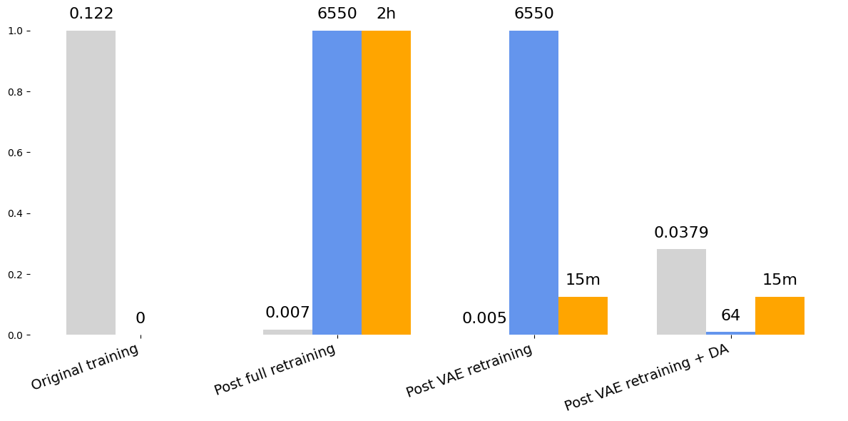
We achieved nearly a 70% reduction in energy distance while using only 1% of actual new data. Model convergence is usually achieved after just a few training epochs, allowing for rapid, near-real-time adaptation. In practice, however, prediction of the first moment converges much earlier — within seconds — providing real-time fine-tuning capability when estimates of variance and uncertainty are not required. After just 30 seconds of fine-tuning using data assimilation, the model’s error reaches its minimum. Figure 16 demonstrates this rapid correction, with the forecasted energy signal following the fine-tuning process. This result highlights the effectiveness and responsiveness of the approach, especially when only the model prediction needs updating.

Figure 16: Kinetic energy forecast after 30s of fine-tuning with DA

Regarding uncertainty quantification, the use of assimilated rather than full-state data has negligible impact on the uncertainty distribution across the flow field. Section 6.1 provides a deeper analysis of the impact of DA on the uncertainty estimate and offers a justification for neglecting the additional uncertainty induced by the Kalman filter, measurable with the second moment of the analysis ensemble.

6.1 Kalman Uncertainties

The Kalman filter produces an analysis ensemble that inherently carries a certain degree of uncertainty. The covariance of this ensemble provides a quantitative measure of that uncertainty. Therefore, an important question is whether the model’s uncertainty estimate should explicitly incorporate the uncertainty already present in the Kalman filter’s analysis ensemble. In other words, should the retraining process account not only for the first statistical moment (the mean state) but also for the second moment (the covariance) of the assimilated data? In our current framework, we enforce agreement between the model’s mean prediction and the analysis-ensemble mean, thereby aligning the first moments. The remaining issue is whether we should also align the second moments by producing stochastic predictions whose covariance captures both the model’s intrinsic uncertainty and the aleatoric uncertainty introduced by the Kalman filter.

The following section demonstrates that such an additional treatment of the second moment is not required in our framework. Note, however, that other works (e.g. [bocquet_2]) include the second moment in their retraining objective by penalizing or rewarding more confident states through their loss formulation (Equation 6). Unlike our stochastic framework, their strategy is deterministic; yet this highlights that properly accounting for Kalman filter uncertainties remains crucial for building a trustworthy Machine Learning–DA hybrid system.

Encoder Definition

We define the encoder operator $\mathcal{E}$, which maps a high-dimensional physical state to a probabilistic latent representation parameterized by its mean and (diagonal) covariance:

$$\mathcal{E}:\mathbb{R}^{m}\rightarrow\mathbb{R}^{2\times p},\qquad\mathcal{E}(\psi)=\big(\mu_{\theta},\mathrm{diag}(\Lambda_{\theta})\big),\qquad\text{with }p\ll m.$$ (7)

The subscript $\theta$ denotes the network parameters. The vector $\mathrm{diag}(\Lambda_{\theta})$ represents the encoder-predicted variance (the second statistical moment). Conceptually, this variance acts as a proxy for the diagonal entries of the true posterior covariance matrix of $p(z\,|\,\psi)$, where $z$ denotes the latent coordinates. The VAE therefore assumes statistical independence across latent dimensions, neglecting off-diagonal covariance components.

First-Moment Matching

Fine-tuning enforces alignment between the first moments: the mean forecast of the model is matched to the mean of the analysis ensemble, denoted by $X^{a}$. This matching is achieved via the loss function in Equation 5. The next step is to verify that the model remains insensitive to the covariance structure of the analysis ensemble.

Definition of the Analysis Ensemble

Let the updated (assimilated) forecast ensemble be

$$\psi^{a}=\{\psi_{1}^{a},\psi_{2}^{a},\dots,\psi_{N}^{a}\}\in\mathbb{R}^{N\times m},$$

where each $\psi_{i}^{a}$ is a sample drawn from the posterior distribution

$$\psi_{i}^{a}\sim\mathcal{N}(X^{a},P^{a}),$$

and where

$$X^{a}=\frac{1}{N}\sum_{i=1}^{N}\psi_{i}^{a},\qquad P^{a}=\mathrm{Cov}(\psi^{a})$$

denote the ensemble mean and its empirical covariance, respectively.

Latent-Space Representation

Each ensemble member $\psi_{i}^{a}$ is mapped into the latent space via the encoder:

$$\mathcal{E}:\psi_{i}^{a}\mapsto z_{i}^{a},\quad z_{i}^{a}\in\mathbb{R}^{p},$$ (8)

yielding a latent ensemble distributed as

$$z^{a}\sim\mathcal{N}(\mu_{z}^{a},\Sigma_{z}^{a}),$$ (9)

with empirical mean and covariance

$$\mu_{z}^{a}=\frac{1}{N}\sum_{i=1}^{N}z_{i}^{a},\qquad\Sigma_{z}^{a}=\frac{1}{N-1}\sum_{i=1}^{N}(z_{i}^{a}-\mu_{z}^{a})(z_{i}^{a}-\mu_{z}^{a})^{\top}.$$

This ensemble thus defines fixed first and second moments in the latent space, providing a reference distribution for the autoencoder to reproduce.

Variational Encoding

Within the VAE framework, the encoder outputs a Gaussian approximation to the posterior:

$$\mathcal{E}:X^{a}\mapsto\hat{z}_{\theta}^{a}\sim\mathcal{N}\!\left(\mu_{\theta}^{a},\mathrm{diag}(\Lambda_{\theta}^{a}\right)),$$ (10)

where $\mu_{\theta}^{a}\in\mathbb{R}^{p}$ is the predicted latent mean, and $\Lambda_{\theta}^{a}\in\mathbb{R}^{p\times p}$ is the predicted (diagonal) latent covariance.

Since the latent means are already aligned ($\mu_{\theta}^{a}=\mu_{z}^{a}$; see Section 5.1), our focus now shifts to ensuring that the predicted covariance $\Lambda_{\theta}^{a}$ approximates the latent covariance structure $\Sigma_{z}^{a}$ obtained from the assimilated ensemble. We thus compare:

$$\Sigma_{z}^{a}=\begin{pmatrix}\sigma_{1}^{2}&\sigma_{1}\sigma_{2}&\cdots&\sigma_{1}\sigma_{p}\\ \sigma_{2}\sigma_{1}&\sigma_{2}^{2}&\cdots&\sigma_{2}\sigma_{p}\\ \vdots&\vdots&\ddots&\vdots\\ \sigma_{p}\sigma_{1}&\sigma_{p}\sigma_{2}&\cdots&\sigma_{p}^{2}\end{pmatrix},\qquad\Lambda_{\theta}^{a}=\begin{pmatrix}\lambda_{1}&0&\cdots&0\\ 0&\lambda_{2}&\cdots&0\\ \vdots&\vdots&\ddots&\vdots\\ 0&0&\cdots&\lambda_{p}\end{pmatrix},$$

where each $\lambda_{i}$ is directly predicted by the encoder.

Minimization Problem

If the VAE is designed to fit both the first and second statistical moments of the assimilated latent distribution, it must minimize the following constrained optimization problem:

$$\Lambda_{\theta}^{a*}=\arg\min_{\Lambda_{\theta}^{a}}D_{\mathrm{KL}}\!\left(\mathcal{N}(\mu_{z}^{a},\Sigma_{z}^{a})\,\|\,\mathcal{N}(\mu_{\theta}^{a},\Lambda_{\theta}^{a})\right)\quad\text{subject to}\quad(\Lambda_{\theta}^{a})_{ij}=0\;\;\text{for }i\neq j.$$ (11)

The Kullback–Leibler divergence between two multivariate normal distributions is:

$$D_{\mathrm{KL}}\big(\mathcal{N}(\mu_{z}^{a},\Sigma_{z}^{a})\,\|\,\mathcal{N}(\mu_{\theta}^{a},\Lambda_{\theta}^{a})\big)=\tfrac{1}{2}\Big[ \log\tfrac{\det\Lambda_{\theta}^{a}}{\det\Sigma_{z}^{a}}-p+\mathrm{tr}\!\big((\Lambda_{\theta}^{a})^{-1}\Sigma_{z}^{a}\big)+(\mu_{\theta}^{a}-\mu_{z}^{a})^{\top}(\Lambda_{\theta}^{a})^{-1}(\mu_{\theta}^{a}-\mu_{z}^{a})\Big].$$ (12)

Since the first moments are already matched ($\mu_{\theta}^{a}=\mu_{z}^{a}$), this simplifies to:

$$D_{\mathrm{KL}}=\tfrac{1}{2}\left[\log\tfrac{\det\Lambda_{\theta}^{a}}{\det\Sigma_{z}^{a}}-p+\mathrm{tr}\!\big((\Lambda_{\theta}^{a})^{-1}\Sigma_{z}^{a}\big)\right].$$ (13)

we obtain:

$$D_{\mathrm{KL}}=\tfrac{1}{2}\left[\log\tfrac{\prod_{i=1}^{p}\lambda_{i}}{\det\Sigma_{z}^{a}}-p+\sum_{i=1}^{p}\tfrac{\sigma_{i}^{2}}{\lambda_{i}}\right].$$ (14)

Ignoring constants, the minimization reduces to:

$$\min_{\lambda_{i}>0}\;f(\lambda_{i})=\log\!\left(\prod_{i=1}^{p}\lambda_{i}\right)+\sum_{i=1}^{p}\frac{\sigma_{i}^{2}}{\lambda_{i}}.$$

Setting the derivative to zero gives:

$$\frac{\partial f}{\partial\lambda_{i}}=\frac{1}{\lambda_{i}}-\frac{\sigma_{i}^{2}}{\lambda_{i}^{2}}=0\quad\Rightarrow\quad\lambda_{i}^{*}=\sigma_{i}^{2}.$$

$$\left.\frac{\partial^{2}f}{\partial\lambda_{i}^{2}}\right|_{\lambda_{i}=\lambda_{i}^{*}}=-\frac{1}{\lambda_{i}^{2^{*}}}+\frac{2\sigma_{i}^{2}}{\lambda_{i}^{3^{*}}}=\frac{2\sigma_{i}^{2}-\lambda_{i}^{*}}{\lambda_{i}^{3^{*}}}$$

Since $\sigma_{i}^{2}>0$ and $\lambda_{i}^{*}=\sigma_{i}^{2}$, we have

$$\left.\frac{\partial^{2}f}{\partial\lambda_{i}^{2}}\right|_{\lambda_{i}=\lambda_{i}^{*}}>0,$$

which shows that the function $f$ is locally convex around $\lambda^{*}$, making $\lambda^{*}$ a local minimum. Moreover, considering the monotonicity of the $\log$ and inverse functions together with the behaviour of $f(\lambda)$ tending to infinity as $\lambda_{i}\to 0^{+}$ or $\lambda_{i}\to+\infty$, we conclude that $f$ admits a unique global minimum. Thus, the optimal diagonal covariance approximation is:

$$\Lambda_{\theta}^{a*}=\mathrm{diag}(\Sigma_{z}^{a}).$$

Interpretation

This result implies that if encoding the mean of the analysis ensemble, $X^{a}$, yields variance components $\lambda_{\text{VAE}}=\mathrm{diag}(\Lambda_{\theta}^{a})$ that, at each time step, are equal to the diagonal entries of the covariance matrix obtained by encoding each ensemble member individually, then the model’s second statistical moment faithfully captures that of the Kalman filter. Formally,

$$\lambda_{\text{VAE}}^{*}=\arg\min_{\lambda_{\text{VAE}}}\left\|\lambda_{\text{VAE}}-\mathrm{diag}\!\left(\mathrm{Cov}\!\left[\mathcal{E}(\psi_{i}^{a})\right]\right)\right\|.$$ (15)

In our experimental setup with $p=4$, we can confirm that the optimization problem defined in Equation 15 is successfully solved. Figure 17 presents a comparison of the $p=4$ signals, plotted two by two, between the true latent variances obtained from the ensemble and the corresponding variance estimates produced by the encoder when applied to the ensemble mean.

Figure 17: Comparison of $p$ pairs of variance signals: true latent variances (from encoding the ensemble) versus variance predictions from the encoder (based on the ensemble mean).

These results demonstrate that the VAE effectively captures the uncertainty structure of the analysis ensemble without requiring the explicit inclusion of second-moment terms in the loss function. This statement holds true within our experimental setup, but it is not necessarily guaranteed to generalize to other systems. However, as a rule of thumb, when the analysis ensemble variance remains small compared with the system’s total energy, such an approximation can be reasonably made. Since we only consider the diagonal components of the analysis ensemble covariance matrix, that is, its variance, this uncertainty can be interpreted as a form of additive noise. Consequently, the model can effectively suppress this noise through its inherent denoising capability.

Finally it should be noted that even though the noise does not affect model predictions, it can reduce the model’s overall confidence. To address this, smoothing filters could be applied prior to fine-tuning to effectively denoise the assimilated data, potentially improving the performance of the DA–DL framework. However, designing such filters remains challenging for high-dimensional, highly nonlinear systems, particularly when the predictive model operates as a black box that is incompatible with classical smoothers such as the Rauch–Tung–Striebel smoother.

7 Conclusion

This work introduces an efficient fine-tuning methodology. Efficiency is achieved through two key mechanisms: (i) fine-tuning only a designated subcomponent of the model, which substantially reduces training time, and (ii) incorporating sparse datasets during the retraining process.

Firstly, by only adapting the components of the model that require correction, namely, the parts of the learned manifold that shift between nearby Reynolds regimes, we can avoid making unnecessary updates to the underlying dynamics, which remain largely unchanged. Empirically, when flow conditions differ only moderately, the manifold deforms while the trajectory on it remains preserved, enabling rapid and inexpensive retraining. Secondly, since acquiring data is costly, we demonstrate that accurate adaptation can be achieved using a very small amount of data via assimilation enabled by ensemble Kalman filters. These leverage the stochastic nature of our reduced order model, resulting in a symbiotic relationship between data assimilation and machine learning. The model’s stochastic and Gaussian properties benefit the assimilation process, while assimilation generates new data to retrain and improve the model.

This selective adaptation results in near-real-time convergence for both the first and second moments, as well as real-time updates within seconds when only the first moment is required. Ultimately, by using just one percent of the full-state data, acquired strategically via targeted sensor placement, we can reduce prediction error by up to 70%, representing an excellent trade-off between performance and fine-tuning cost.

While data assimilation enables this efficient correction, it also introduces noise that can reduce the model’s confidence. This decreased certainty arises from the assimilation noise itself rather than from the intrinsic EnKF uncertainty, and therefore does not necessitate incorporating ensemble variance into the fine-tuning step. In principle, smoothing filters could be used to mitigate this noise and improve robustness further.

Overall, the proposed framework strikes a favorable balance between accuracy, computational cost, and data requirements, providing a practical and scalable avenue for fast domain adaptation in learned dynamical models.

Appendix A Appendix

A.1 ROM architecture

Parameter	Value
Data parametric dimensions (train)	2
Data parametric dimensions (validation/test)	7
Time dimension	1516
Spatial dimensions	$131\times 100\div 4=3275$
Flows	$u,v$
Input dimension	$3275\times 2=6550$
Latent dimensions	4
Transformer hidden dimensions	64
Kullback-Leibler regularization	$3\times 10^{-4}$
Attention blocks	1
Attention heads	8
Prediction horizon	10
Lookback window	9

Table 4: Model and data configuration parameters.

A.2 Sensor location

Conventional methods in data compression, sparse reconstruction, and sparse optimization involve estimating the high-dimensional state using low-rank approximations. For instance, when dealing with flow past an obstacle, the data can often be accurately represented using a few eigenmodes through Singular Value Decomposition (SVD). By employing tailored sensing, we can optimize the placement of observations using a subsampling matrix that captures as much information as possible about the full state signal in the most sparse manner, making it a classic optimization problem. The low rank approximation of a full-state, high dimensional, potentially noisy vector $x\in\mathbb{R}^{T,m}$ with $T$ and $m$ the time dimension and spatial dimension respectively is derived below.
Starting from the Singular Value Decomposition (SVD), we write :

$$x=U\Sigma V^{T},$$ (16)

where $U\in\mathbb{R}^{m\times k}$ contains the spatial modes, $\Sigma\in\mathbb{R}^{k\times k}$ is the diagonal matrix of singular values, and $V\in\mathbb{R}^{T\times k}$ holds the temporal coefficients, with $k\leq\min(T,D)$. We define $\Psi=U\Sigma$, which combines the spatial structures with their energetic weights.

$$x\approx x_{r}=\Psi_{r}a$$ (17)

where the subscript $r$ indicates the rank of truncation in the eigenbase, $a$ indicates the ”mixture” of active modes. We also define the sub-sampling operator $H\in\mathbb{R}^{p\times n}$, which defines the locations of the $p$ sensors across the full state data $x\in\mathbb{R}^{n}$. The observations $y$ are therefore defined as:

$$y=Hx$$ (18)

Combining equations 17 and 18 implies that:

$$y=H\Psi_{r}a$$ (19)

This means that we could theoretically reconstruct the full state data by simply computing $a$ from the sensors observations via:

$$a=\begin{cases}(H\Psi_{r})^{-1}y&\text{if }n=r\\ (H\Psi_{r})^{\dagger}y&\text{if }n>r\end{cases}$$ (20)

In practice, the reconstruction of $a$ heavily depends on the structure of $H$. Specifically, it is crucial to ensure that minor noise in $y$ does not drastically affect the signal reconstruction. Ensuring that small variations in $y$ result in small variations in the full state reconstruction is a problem known as condition number minimization. This means that the inversion of $H\Psi_{r}$ should be well-conditioned and not rank-deficient.
Equivalently, we seek the structure of $H$ that maximizes the determinant of $H\Psi_{r}$:

$$H=\arg\max_{H}\left|\det(H\Psi_{r})\right|$$ (21)

leading to,

$$H=\arg\max_{H}\prod_{i=1}^{r}\lambda_{i}(H\Psi_{r})$$ (22)

where $\lambda_{i}$ are the eigenvalues of the matrix product $H\Psi_{r}$. This remains a combinatorial NP-hard problem, but a greedy approximation of $H$ can be found from the pivot matrix $C$ in the QR factorization of the basis matrix $\Psi$:

$$\Psi_{r}^{T}C^{T}=QR$$ (23)

where $C$ is the pivot matrix containing $p=r$ non-zero entries, $Q$ is an orthogonal, unitary matrix and $R$ is an upper triangular matrix. This latter statement holds true as long as $p=r$, but other formulations can be derived in the case where $p>r$. The pivot matrix $C$ iteratively finds the rows of $\Psi_{r}$ with the highest $l_{2}$-norm, the orthogonal projection onto this pivot row is then subtracted from the other rows before repeating the procedure. We can then have a sense of why $C$ is the best greedy approximation for $H$ as it finds the placements with the highest modal variance, thus carrying the most information about each mode. This iterative process ensures that each diagonal entry in $R$ is as large as possible given the preceding entry. Since $R$ is a triangular matrix, we have:

$$\det(\Psi_{r}^{T}C_{r}^{T})=\det(\Psi_{r}C_{r})=\prod_{i=1}^{r=p}R_{ii}\approx\max_{H}\left|\det(H\Psi_{r})\right|$$ (24)