The transient behavior of superconducting
multi-cell accelerating cavities.

Abstract

We employ an equivalent-circuit model of a multi-cell cavity to explore its time-dependent behavior in order to understand differences between the multi-cell model and the commonly-used model of a single-cell resonator. Furthermore, we address tolerances that arise from manufacturing imperfections.

1 Introduction

In most simulations of the transient behavior of multi-cell superconducting acceleration structures the cavity is represented by a single resonator that consists of a discrete resistor $R$, inductor $L$, and capacitance $C$ [1, 2]. In reality, however, the individual cells that constitute the cavity should be treated as individual but coupled resonators, each having its specific resonance-frequency detuning, $Q$-value, and shunt impedance $R$. Only for the analysis of the supported eigenmodes in multi-cell cavities, the cells are considered as coupled resonators [3]. This analysis is mostly static though some time-dependent effects are mentioned in [4]. In this report, we present a comprehensive analysis of multi-cell cavities and discuss the impact of cavity-fabrication imperfections on their time-dependent behavior.

Figure 1: Multi-cell cavity based on parallel-circuit RLC resonators, coupled via capacitors $\hat{C}$, and driven by a generator with input impedance $Z_{0}$.

Figure 1 illustrates our model. The generator with internal impedance $Z_{0}$ provides a current $I_{g}$ that is transported to the cavity by a matched transmission line. The input power is fed to the first cell with an input coupler that is modeled as a transformer with winding ratio $n$. Each of the individual cells is represented as an independent RLC circuit and adjacent cells are coupled via capacitors $\hat{C}$. Additionally, the first and last cell experience the coupling to the beam pipe, here modeled by the capacitors labeled $C_{a}$ and $C_{b}$. We also indicate the beam current $I_{c}$ that passes through all cells and excites fields inside the cells, though in this note we do not consider this effect and focus on the behavior of the cavity without beam. In particular, we address variations among cells and how they affect the forward current $I^{+}_{L}$ and the backward current $I^{-}_{L}$ measured by a directional coupler just upstream of the coupler as well as a field probe connected to the last cell that measures the cavity voltage $V_{n}$. Reference planes on either side of the coupler are depicted as dashed lines. The voltages and currents are related by the transformer ratio $V_{1}=nV_{L}$ and $I_{1}=I_{L}/n$ and consequently the impedances $Z_{0}=Z_{L}=V_{L}/I_{L}$ and $Z_{g}=V_{1}/I_{1}$ are related by $Z_{g}=n^{2}Z_{L}$.

Before addressing the fully time-dependent problem, we briefly address the steady state of the bare multi-cell cavity. This analysis follows the discussion in [3] and helps us to determine values for the beam pipe capacitances $C_{a}$ and $C_{b}$ as well as the supported eigenfrequencies and corresponding eigenmodes in the cavity. In contrast to the discussion in [3, 4], which is based on series-resonator circuits, we use parallel circuits.

2 Steady-state

Figure 2: Bare multi-cell cavity in which coupling to the generator and the resistors are omitted. Note, however, the capacitors $C_{a}$ and $C_{b}$ that represent coupling to the beam pipe.

In order to determine $C_{a}$ and $C_{b}$ we analyze the simplified model shown in Figure 2 where the generator and coupler are omitted. Moreover, all capacitances between the cavities are assumed equal and that $C_{a}=C_{b}$ owing to the forward-backward symmetry of the simplified model. We add a grounding symbol to indicate the reference level for voltage measurements.

We assume that the system oscillates with frequency $\omega$ such that we can use the following impedances $Z_{C}=1/i\omega C$ and $Z_{L}=i\omega L$ to characterize the capacitor and inductor, respectively. For the current balance at the first node with voltage $V_{1}$ we thus find

$$0=I_{1}-I_{2}+I_{LC}=i\omega C_{a}V_{1}-i\omega\hat{C}(V_{2}-V_{1})+\left(i\omega C+\frac{1}{i\omega L}\right)V_{1}\ ,$$ (1)

where $I_{LC}$ is the current that flows from ground to the node labeled $V_{1}$. Diving this equation by $i\omega C$ and introducing the abbreviations $\kappa_{a}=C_{a}/C$ and $\hat{\omega}^{2}=1/LC$ we arrive at

$$\left(1+\kappa+\kappa_{a}\right)V_{1}-\kappa V_{2}=\frac{\hat{\omega}^{2}}{\omega^{2}}V_{1}\ .$$ (2)

Likewise, the current balance at cell $j$ leads us to

$$0=I_{j}-I_{j-1}+I_{LC}=i\omega\hat{C}(V_{j}-V_{j-1})-i\omega\hat{C}(V_{j+1}-V_{j})+\left(i\omega C+\frac{1}{i\omega L}\right)V_{j}\ .$$ (3)

Dividing by $i\omega C$ and some rearranging then gives us

$$-\kappa V_{j-1}+(1+2\kappa)V_{j}-\kappa V_{j+1}=\frac{\hat{\omega}^{2}}{\omega^{2}}V_{j}\ .$$ (4)

Repeating the analysis for the right-most node labeled $V_{n}$ finally results in

$$0=i\omega\hat{C}(V_{n}-V_{n-1})+\left(i\omega C+\frac{1}{i\omega L}\right)V_{j}-i\omega C_{a}(0-V_{n})$$ (5)

and, after introducing abbreviations, leads to

$$-\kappa V_{n-1}+(1+\kappa+\kappa_{a})V_{n}=\frac{\hat{\omega}^{2}}{\omega^{2}}V_{n}\ .$$ (6)

Jointly, equations 2, 4, and 6 can be cast into the following eigenvalue equation

$$\left(\begin{array}[]{ccccc}1+\kappa+\kappa_{a}&-\kappa&0&0&0\\ -\kappa&1+2\kappa&-\kappa&0&0\\ 0&-\kappa&1+2\kappa&-\kappa&\\ 0&0&-\kappa&1+2\kappa&-\kappa\\ 0&0&0&-\kappa&1+\kappa+\kappa_{a}\end{array}\right)\left(\begin{array}[]{c}V_{1}\\ V_{2}\\ V_{3}\\ V_{4}\\ V_{5}\end{array}\right)=\frac{\hat{\omega}^{2}}{\omega^{2}}\left(\begin{array}[]{c}V_{1}\\ V_{2}\\ V_{3}\\ V_{4}\\ V_{5}\end{array}\right)$$ (7)

where we assumed that $n=5$. Generalizing to other numbers of cells $n$ is trivial.

We follow [3] and require the $\pi$-mode to produce alternating signs of voltages in adjacent cells: $(V_{1},V_{2},V_{3},\dots)=(1,-1,1,\dots)$. Imposing this requirement on Equation 7 and considering the first two rows leads to the conditions

$$1+2\kappa+\kappa_{a}=\frac{\hat{\omega}^{2}}{\omega_{\pi}^{2}}\qquad\mathrm{and}\qquad-1-4\kappa=-\frac{\hat{\omega}^{2}}{\omega_{\pi}^{2}}\ .$$ (8)

Solving for $\kappa_{a}$ and $\hat{\omega}^{2}/\omega_{\pi}^{2}$ leads to

$$\kappa_{a}=2\kappa\qquad\mathrm{and}\qquad\omega_{\pi}=\frac{\hat{\omega}}{\sqrt{1+4\kappa}}\ .$$ (9)

We need to point out that in our model the $\pi$-mode frequency lies below the cell’s resonance frequency $\hat{\omega}$, which is an artefact of using a parallel-resonator circuit. With a series-resonator circuit the $\pi$-mode frequency is above $\hat{\omega}$.

Now that we know what $\kappa_{a}$ should be, we insert it in Equation 7 and find the following, now properly matched, eigenvalue equation

$$\left(\begin{array}[]{ccccc}1+3\kappa&-\kappa&0&0&0\\ -\kappa&1+2\kappa&-\kappa&0&0\\ 0&-\kappa&1+2\kappa&-\kappa&\\ 0&0&-\kappa&1+2\kappa&-\kappa\\ 0&0&0&-\kappa&1+3\kappa\end{array}\right)\left(\begin{array}[]{c}V_{1}\\ V_{2}\\ V_{3}\\ V_{4}\\ V_{5}\end{array}\right)=\frac{\hat{\omega}^{2}}{\omega^{2}}\left(\begin{array}[]{c}V_{1}\\ V_{2}\\ V_{3}\\ V_{4}\\ V_{5}\end{array}\right)$$ (10)

that we inspect further to determine all eigenfrequencies and eigenmodes. As mentioned before, the corresponding equations in [3] are derived from a series-circuit model as opposed to the parallel-circuit model employed here. Therefore, even though the structure of Equation 10 resembles the corresponding equation from [3], the definition of constants differs and therefore no one-to-one correspondence is possible.

Figure 3: Modes and eigenvalues of a five-cell cavity with $\kappa=0.01$.

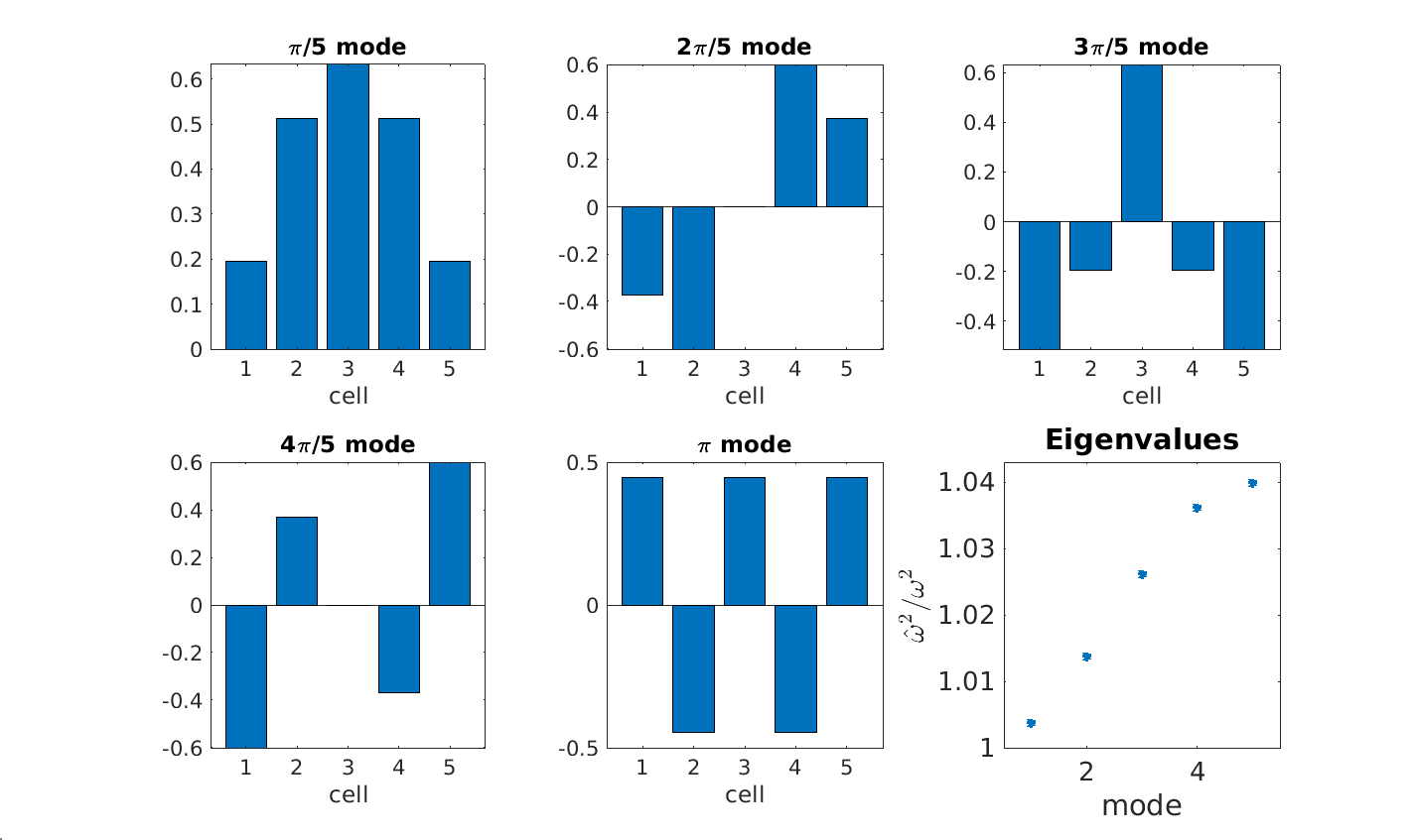
As a matter of fact, the high degree of symmetry of the matrix in Equation 10 permits an analytical representation of the eigenvalues and eigenvalues, which is used in [3], but we do not duplicate those results. Instead, we calculate the corresponding quantities numerically using Matlab. Figure 3 shows the five eigenmodes for $\kappa=0.01$ in the plots labeled $n\pi/5$-mode and the corresponding eigenvalues in the bottom-right plot. Here mode 1 refers to the $\pi/5$-mode and mode 2 to the $2\pi/5$-mode. In particular, we see that the largest eigenvalue for mode 5 corresponds to the $\pi$-mode whose numerical value is $\hat{\omega}^{2}/\omega_{\pi}^{2}=1.04$, which agrees with Equation 9.

If we excite the different modes with their respective frequencies, the combined excitation pattern can be shaped to peak in different cells. This feature is exploited when plasma-processing a cavity [5]. It allows us to locally excite a plasma in a particular cell to clean it.

Figure 4: Eigenvalues as function of an error $\Delta\kappa_{2}$ (left) and the relative frequency shift $\Delta\omega_{\pi}/\omega_{\pi}$ of the $\pi$-mode (right).

It is instructive to explore the sensitivity of the eigenfrequencies as a function of an error of the coupling $\kappa$ in one cell. The right-hand plot in Figure 4 shows the eigenvalues if the coupling between the second and third cell $\kappa_{2}$ varies. The range chosen is rather large; $\Delta\kappa_{2}=-0.01$ corresponds to absent coupling and $\Delta\kappa_{2}=0.01$ corresponds to a doubling of the design value. We observe that especially the eigenvalue of the $\pi$-mode increases substantially, especially for positive values of $\Delta\kappa_{2}$. The right hand-hand plot shows the relative frequency change $\Delta\omega_{\pi}/\omega_{\pi}$ that is derived from the eigenvalue. It varies by almost one percent in the range chosen. The slope of the curve around $\Delta\kappa_{2}=0$ gives us the sensitivity eigenfrequency with respect to $\Delta\kappa_{2}$. From a fit to scanning $\Delta\kappa_{2}$ over a smaller range, we find

$$\Delta\left(\Delta\omega_{\pi}/\omega_{\pi}\right)=-0.38\,\Delta\kappa_{2}\ ,$$ (11)

which is large, considering the very small bandwidth of superconducting cavities. An error of $\Delta\kappa_{2}=10^{-4}$ thus moves the frequency outside the bandwidth of the cavity.

The analysis in this section is purely static. In the next sections we will, however, extend it to account for transient phenomena. In that context we also introduce specific imperfections to individual cells, which will allow us to explore their consequences.

3 Model

Let us now consider the current $I_{j}$ that flows through the $RLC$-branch of cell j in the middle of the cavity. The first and last cells need special considerations and we will come back to them later. The current balance at the point labeled $V_{j}$ is given by the sum of the currents passing through $R$, $L$ and $C$ individually. We thus find [6]

$$0=I_{j}-I_{j+1}+\frac{V_{j}}{R_{j}}+\frac{1}{L_{j}}\int V_{j}dt+C_{j}\frac{dV_{j}}{dt}$$ (12)

The currents $I_{j}$ and $I_{j+1}$ pass through the capacitors $\hat{C}_{j-1}$ and $\hat{C}_{j}$, respectively and are determined by the difference of voltages $V_{j}$ in the adjacent cells

$$I_{j}=\hat{C}_{j-1}\left[\frac{dV_{j}}{dt}-\frac{dV_{j-1}}{dt}\right]\qquad\mathrm{and}\qquad I_{j+1}=\hat{C}_{j}\left[\frac{dV_{j+1}}{dt}-\frac{dV_{j}}{dt}\right]\ .$$ (13)

Inserting in Equation 12 results in

$$0=-\hat{C}_{j-1}\frac{dV_{j-1}}{dt}-\hat{C}_{j+1}\frac{dV_{j+1}}{dt}+\frac{V_{j}}{R_{j}}+\frac{1}{L_{j}}\int V_{j}dt+\left(C_{j}+\hat{C}_{j-1}+\hat{C}_{j+1}\right)\frac{dV_{j}}{dt}\ .$$ (14)

Dividing by $C_{j}$ and introducing the abbreviations $\kappa^{\prime}_{j}=\hat{C}_{j-1}/C_{j}$ and $\kappa_{j}=\hat{C}_{j+1}/C_{j}$ turns this equation into

$$0 = -\kappa^{\prime}_{j}\frac{dV_{j-1}}{dt}-\kappa_{j}\frac{dV_{j+1}}{dt}+\frac{V_{j}}{R_{j}C_{j}}+\frac{1}{L_{j}C_{j}}\int V_{j}dt+\left(1+\kappa^{\prime}_{j}+\kappa_{j}\right)\frac{dV_{j}}{dt}$$ (15)

$$= -\kappa^{\prime}_{j}\frac{dV_{j-1}}{dt}-\kappa_{j}\frac{dV_{j+1}}{dt}+\frac{\hat{\omega}_{j}}{Q_{j}}V_{j}+\hat{\omega}_{j}^{2}\int V_{j}dt+\left(1+\kappa^{\prime}_{j}+\kappa_{j}\right)\frac{dV_{j}}{dt}\ ,$$

where we use the abbreviations $1/L_{j}C_{j}=\hat{\omega}_{j}^{2}$ and $R_{j}C_{j}=Q_{j}/\hat{\omega}_{j}$ in the second equality. At this point we introduce the slowly varying amplitude $\tilde{V}_{j}$ of $V_{j}=\tilde{V}_{j}e^{i\omega t}$, which allows us to write [6]

$$\frac{dV_{j}}{dt}=e^{i\omega t}\left[i\omega\tilde{V}_{j}+\frac{d\tilde{V}_{j}}{dt}\right]\qquad\mathrm{and}\qquad\int V_{j}dt=\frac{e^{i\omega t}}{\omega^{2}}\left[-i\omega\tilde{V}_{j}+\frac{d\tilde{V}_{j}}{dt}\right]\ ,$$ (16)

for $j=1,\dots,n$. Here we neglect the second derivative $d^{2}\tilde{V}_{j}/dt^{2}$ and $\omega$ is the frequency at which the generator operates. After substituting in Equation 15, canceling the common exponential $e^{i\omega t}$, and some rearranging, we obtain

$$0 = -\kappa^{\prime}_{j}\frac{d\tilde{V}_{j-1}}{dt}-\kappa_{j}\frac{d\tilde{V}_{j+1}}{dt}+\left(1+\kappa^{\prime}_{j}+\kappa_{j}+\frac{\hat{\omega}_{j}^{2}}{\omega^{2}}\right)\frac{d\tilde{V}_{j}}{dt}$$

$$\quad+\frac{\hat{\omega}_{j}}{Q_{j}}\tilde{V}_{j}+i\omega\left[-\kappa^{\prime}_{j}\tilde{V}_{j-1}-\kappa_{j}\tilde{V}_{j+1}+\left(1+\kappa^{\prime}_{j}+\kappa_{j}-\frac{\hat{\omega}_{j}^{2}}{\omega^{2}}\right)\tilde{V}_{j}\right]\ .$$

The quantity in the square brackets turns out to be the equivalent of Equation 4 provided the all $\kappa^{\prime}_{j}$ and $\kappa_{j}$ are equal. The value of $\omega$ for which this bracket vanishes thus determines the eigenvalues of the matrix in Equation 7 that describe the steady-state of the system, because in that case, also the derivatives of the voltages with respect to time have to vanish. The additional term, proportional to $\hat{\omega}_{j}/Q_{j}$, is due to the finite resistance $R_{j}$ and describes damping. This term is absent in the discussion in Section 2. For future reference, we rewrite Equation 3 in the following way

$$-\kappa^{\prime}_{j}\frac{d\tilde{V}_{j-1}}{dt}+\left(1+\kappa^{\prime}_{j}+\kappa_{j}+\frac{\hat{\omega}_{j}^{2}}{\omega^{2}}\right)\frac{d\tilde{V}_{j}}{dt}-\kappa_{j}\frac{d\tilde{V}_{j+1}}{dt}$$ (18)

$$\quad=-\frac{\hat{\omega}_{j}}{Q_{j}}\tilde{V}_{j}-i\omega\left[-\kappa^{\prime}_{j}\tilde{V}_{j-1}+\left(1+\kappa^{\prime}_{j}+\kappa_{j}-\frac{\hat{\omega}_{j}^{2}}{\omega^{2}}\right)\tilde{V}_{j}-\kappa_{j}\tilde{V}_{j+1}\right]\ ,$$

which separates the terms with the derivatives on the left-hand side of the equality and the rest on the right-hand side.

For the last cell $n$ we start from the current balance on the node labeled $V_{n}$ in Figure 1

$$0=I_{n}-I_{n+1}+\frac{V_{n}}{R_{n}}+\frac{1}{L_{n}}\int V_{n}dt+C_{n}\frac{dV_{n}}{dt}$$ (19)

and express the currents through the voltages in the adjacent nodes

$$I_{n}=\hat{C}_{n-1}\left[\frac{dV_{j}}{dt}-\frac{dV_{j-1}}{dt}\right]\qquad\mathrm{and}\qquad I_{n+1}=C_{b}\left[0-\frac{dV_{n}}{dt}\right]\ ,$$ (20)

where the capacitor $C_{b}$ is connected to ground potential on its other end, which accounts for the zero in the square bracket. Collecting terms and introducing the abbreviations $\kappa^{\prime}_{n}=\hat{C}_{n-1}/C_{n}$ and $\kappa_{b}=C_{b}/C_{n}$ leads to

$$0=-\kappa^{\prime}_{n}\frac{dV_{n-1}}{dt}+\left(1+\kappa^{\prime}_{n}+\kappa_{b}\right)\frac{dV_{n}}{dt}+\frac{\hat{\omega}_{n}}{Q_{n}}V_{n}+\hat{\omega}_{n}^{2}\int V_{n}dt\ ,$$ (21)

where we introduced $1/L_{n}C_{n}=\hat{\omega}_{n}^{2}$ and $R_{n}C_{n}=Q_{n}/\hat{\omega}_{n}$. With the help of Equation 16, and after canceling the common exponential $e^{i\omega t}$, this equation becomes

$$0 = -\kappa^{\prime}_{n}\frac{d\tilde{V}_{n-1}}{dt}+\left(1+\kappa^{\prime}_{n}+\kappa_{b}+\frac{\hat{\omega}_{n}^{2}}{\omega^{2}}\right)\frac{d\tilde{V}_{j}}{dt}$$

$$\quad+\frac{\hat{\omega}_{n}}{Q_{n}}\tilde{V}_{n}+i\omega\left[-\kappa^{\prime}_{n}\tilde{V}_{n-1}+\left(1+\kappa^{\prime}_{n}+\kappa_{b}-\frac{\hat{\omega}_{n}^{2}}{\omega^{2}}\right)\tilde{V}_{n}\right]\ .$$

As before, the quantity in the square bracket corresponds to Equation 6 and gives rise to the bottom row in the matrix from Equation 7. Some rearranging then leads to

$$-\kappa^{\prime}_{n}\frac{d\tilde{V}_{n-1}}{dt}+\left(1+\kappa^{\prime}_{n}+\kappa_{b}+\frac{\hat{\omega}_{n}^{2}}{\omega^{2}}\right)\frac{d\tilde{V}_{j}}{dt}$$ (23)

$$\qquad=-\frac{\hat{\omega}_{n}}{Q_{n}}\tilde{V}_{n}-i\omega\left[-\kappa^{\prime}_{n}\tilde{V}_{n-1}+\left(1+\kappa^{\prime}_{n}+\kappa_{b}-\frac{\hat{\omega}_{n}^{2}}{\omega^{2}}\right)\tilde{V}_{n}\right]\ ,$$

where we also collect the derivatives on the left-hand side.

Finally, we come to the first cell, which is also connected to the coupler on top of the capacitances $\hat{C}_{1}$ and $C_{a}$. The current balance at the node labeled $V_{1}$ for this cell is

$$\frac{I_{g}}{n} = \frac{V_{1}}{n^{2}Z_{0}}+\frac{V_{1}}{R_{1}}+\frac{1}{L_{1}}\int V_{1}dt+\left(C_{1}+C_{a}\right)\frac{dV_{1}}{dt}-I_{2}$$

$$= \frac{I_{g}}{n}+\left(1+\beta\right)\frac{V_{1}}{R_{1}}+\frac{1}{L_{1}}\int V_{1}dt+\left(C_{1}+C_{a}\right)\frac{dV_{1}}{dt}-\hat{C}_{1}\left[\frac{dV_{2}}{dt}-\frac{dV_{1}}{dt}\right]\ ,$$

where we introduce the coupling factor $\beta=R_{1}/n^{2}Z_{0}$. Note that we have to transform the impedance $Z_{0}$ through the transformer to the inside of the cavity, which accounts for the factor $n^{2}$ in the denominator and dividing the generator current $I_{g}$ by $n$ on the “other” side of the transformer. Furthermore, dividing this equation by $C_{1}$ and introducing the abbreviations $\kappa_{1}=\hat{C}_{1}/C_{1}$ and $\kappa_{a}=C_{a}/C_{1}$, we arrive at

$$\frac{1}{C_{1}}\frac{I_{g}}{n}=(1+\beta)\frac{\hat{\omega}_{1}}{Q_{1}}V_{1}+\hat{\omega}_{1}^{2}\int V_{1}dt+\left(1+\kappa_{a}+\kappa_{1}\right)\frac{dV_{1}}{dt}-\kappa_{1}\frac{dV_{2}}{dt}\ .$$ (25)

After using Equation 16 and canceling the common exponential $e^{i\omega t}$, we obtain

$$\frac{1}{C_{1}}\frac{\tilde{I}_{g}}{n} = \left(1+\kappa_{a}+\kappa_{1}+\frac{\hat{\omega}_{1}^{2}}{\omega^{2}}\right)\frac{d\tilde{V}_{1}}{dt}-\kappa_{1}\frac{d\tilde{V}_{2}}{dt}$$

$$\qquad+(1+\beta)\frac{\hat{\omega}_{1}}{Q_{1}}\tilde{V}_{1}+i\omega\left[\left(1+\kappa_{a}+\kappa_{1}-\frac{\hat{\omega}_{1}^{2}}{\omega^{2}}\right)\tilde{V}_{1}-\kappa_{1}\tilde{V}_{2}\right]\ .$$

The square bracket describes Equation 2 and corresponds to the first row of the matrix in Equation 7. Now we introduce the loaded $Q$-value $Q^{\prime}_{L}=Q_{1}/(1+\beta)$ and note that $1/C_{1}=\hat{\omega}_{1}R_{1}/Q_{1}=\hat{\omega}_{1}R_{1}/(1+\beta)Q^{\prime}_{L}$. Here $Q^{\prime}_{L}$ is the loaded $Q$-value for the first cell only. In passing, we point out that instead of $Q_{1}$, the expression $(1+\beta)Q^{\prime}_{L}$ often appears in the literature. After rearranging Equation 3, we arrive at

$$\left(1+\kappa_{a}+\kappa_{1}+\frac{\hat{\omega}_{1}^{2}}{\omega^{2}}\right)\frac{d\tilde{V}_{1}}{dt}-\kappa_{1}\frac{d\tilde{V}_{2}}{dt}$$ (27)

$$\qquad=-\frac{\hat{\omega}_{1}}{Q^{\prime}_{L}}\tilde{V}_{1}-i\omega\left[\left(1+\kappa_{a}+\kappa_{1}-\frac{\hat{\omega}_{1}^{2}}{\omega^{2}}\right)\tilde{V}_{1}-\kappa_{1}\tilde{V}_{2}\right]+\frac{\hat{\omega}_{1}R_{1}}{Q_{1}}\frac{\tilde{I}_{g}}{n}\ .$$

In the absence of coupling we only have a single cell and a single mode with $\omega\approx\hat{\omega}_{1}$ to deal with. In that case, this equation reverts to $2d\tilde{V}_{1}/dt=-(\hat{\omega}_{1}/Q^{\prime}_{L})\tilde{V}_{1}-i\hat{\omega}_{1}\delta_{1}\tilde{V}_{1}+\hat{\omega}_{1}R_{1}/((1+\beta)Q^{\prime}_{L}){\tilde{I}_{g}}/n$ with the detuning $\delta_{1}=\omega/\hat{\omega}_{1}-\hat{\omega}_{1}/\omega$, which agrees with the calculation for a single resonator in [6].

Equations 18, 23, and 27 describe the dynamics for multi-cell cavity when excited by the generator with frequency $\omega$. In the following sections we will consider the most important case, when the cavity is driven such that the $\pi$-mode is excited.

4 Perfect $\pi$-mode cavity

Here we assume that the frequency at which the generator operates is $\omega_{\pi}=\hat{\omega}/\sqrt{1+4\kappa}$, where $\hat{\omega}$ is the design value of a single cell’s resonance frequency and $\kappa$ is the design value of the coupling between adjacent cells. $Q$ is the unloaded quality factor of the cells, all assumed to be equal. With the design values for $\kappa_{a}=\kappa_{b}=2\kappa$ we can transform Equation 27, describing the first cell, into

$$\left(2+7\kappa\right)\frac{d\tilde{V}_{1}}{dt}-\kappa\frac{d\tilde{V}_{2}}{dt} = -\frac{\hat{\omega}}{Q^{\prime}_{L}}\tilde{V}_{1}-i\omega_{\pi}\left[-\kappa\tilde{V}_{1}-\kappa\tilde{V}_{2}\right]+\frac{\hat{\omega}R_{1}}{Q_{1}}\frac{\tilde{I}_{g}}{n}$$

$$= -\frac{\hat{\omega}}{Q^{\prime}_{L}}\tilde{V}_{1}+i\frac{\hat{\omega}\kappa}{\sqrt{1+4\kappa}}\left[\tilde{V}_{1}+\tilde{V}_{2}\right]+\frac{\hat{\omega}R_{1}}{Q_{1}}\frac{\tilde{I}_{g}}{n}\ .$$

with $Q^{\prime}_{L}=Q/(1+\beta)$. Likewise, the equation for cell $j$ with $2\leq j\leq n-1$ in the middle of the cavity is based on Equation 18, which transforms into

$$-\kappa\frac{d\tilde{V}_{j-1}}{dt}+\left(2+6\kappa\right)\frac{d\tilde{V}_{j}}{dt}-\kappa\frac{d\tilde{V}_{j+1}}{dt}$$

$$\qquad\qquad=-\frac{\hat{\omega}}{Q}\tilde{V}_{j}-i\omega_{\pi}\left[-\kappa\tilde{V}_{j-1}-2\kappa\tilde{V}_{j}-\kappa\tilde{V}_{j+1}\right]$$ (29)

$$\qquad\qquad=-\frac{\hat{\omega}}{Q}\tilde{V}_{j}+i\frac{\hat{\omega}\kappa}{\sqrt{1+4\kappa}}\left[\tilde{V}_{j-1}+2\tilde{V}_{j}+\tilde{V}_{j+1}\right]\ .$$

Finally, for the last cell $n$, we utilize Equation 23, which transforms into

$$-\kappa\frac{d\tilde{V}_{n-1}}{dt}+\left(2+7\kappa\right)\frac{d\tilde{V}_{j}}{dt} = -\frac{\hat{\omega}}{Q}\tilde{V}_{n}-i\omega_{\pi}\left[-\kappa\tilde{V}_{n-1}-\kappa\tilde{V}_{n}\right]$$

$$= -\frac{\hat{\omega}}{Q}\tilde{V}_{n}+i\frac{\hat{\omega}\kappa}{\sqrt{1+4\kappa}}\left[\tilde{V}_{n-1}+\tilde{V}_{n}\right]$$

These three equations thus describe the transient behavior of a perfect multi-cell cavity operating in the $\pi$-mode.

For the simulations, we multiply the equation by $\Delta t$, which makes it numerically more stable, because then most factors are of magnitude unity. Moreover, we transform Equations 4, 4, and 4 into the following matrix-valued equation

$$D\frac{d\vec{V}}{dt}\Delta t=-(A-iB)\vec{V}+\frac{\hat{\omega}\Delta tR_{1}}{Q_{1}}\vec{I}$$ (31)

where we used the abbreviations

$$\vec{V} = \left(\tilde{V}_{1},\tilde{V}_{2},\tilde{V}_{3},\tilde{V}_{4},\tilde{V}_{5}\right)^{\top}$$

$$\frac{d\vec{V}}{dt} = \left(\frac{d\tilde{V}_{1}}{dt},\frac{d\tilde{V}_{2}}{dt},\frac{d\tilde{V}_{3}}{dt},\frac{d\tilde{V}_{4}}{dt},\frac{d\tilde{V}_{5}}{dt}\right)^{\top}$$

$$\vec{I} = \left(\tilde{I}_{g}/n,0,0,0,0\right)^{\top}$$

$$D = \left(\begin{array}[]{ccccc}2+7\kappa&-\kappa&0&0&0\\ -\kappa&2+6\kappa&-\kappa&0&0\\ 0&-\kappa&2+6\kappa&-\kappa&0\\ 0&0&-\kappa&2+6\kappa&-\kappa\\ 0&0&0&-\kappa&2+7\kappa\end{array}\right)$$ (37)

$$A = \mathop{\mathrm{diag}}\left((1+\beta)\frac{\hat{\omega}\Delta t}{Q},\frac{\hat{\omega}\Delta t}{Q},\frac{\hat{\omega}\Delta t}{Q},\frac{\hat{\omega}\Delta t}{Q},\frac{\hat{\omega}\Delta t}{Q}\right)$$

$$B = \frac{\hat{\omega}\Delta t\kappa}{\sqrt{1+4\kappa}}\left(\begin{array}[]{ccccc}1&1&0&0&0\\ 1&2&1&0&0\\ 0&1&2&1&0\\ 0&0&1&2&1\\ 0&0&0&1&1\end{array}\right)\ .$$ (43)

We further manipulate the system by introducing real and imaginary parts of voltages and currents

$$\vec{V}=\vec{V}_{r}+i\vec{V}_{i}\qquad\mathrm{and}\qquad\vec{I}=\vec{I}_{r}+i\vec{I}_{i}\ .$$ (44)

This transforms Equation 31 into

$$\left(\begin{array}[]{cc}D&0_{5}\\ 0_{5}&D\end{array}\right)\left(\begin{array}[]{c}\frac{d\vec{V}_{r}}{dt}\\ \frac{d\vec{V}_{i}}{dt}\end{array}\right)\Delta t=-\left(\begin{array}[]{rr}A&B\\ -B&A\end{array}\right)\left(\begin{array}[]{c}\vec{V}_{r}\\ \vec{V}_{i}\end{array}\right)+\frac{\hat{\omega}\Delta tR_{1}}{Q_{1}}\left(\begin{array}[]{c}\vec{I}_{r}\\ \vec{I}_{i}\end{array}\right)\ ,$$ (45)

where $0_{5}$ is a $5\times 5$ matrix containing only zeros. Here we are now dealing with the 10 real and imaginary parts, or equivalently the I and Q components, of the voltages in the five cells.

The steady-state conditions are given by vanishing time derivatives on the left-hand side and that leads to the steady-state voltages

$$\tilde{V}_{\infty}=\left(\begin{array}[]{c}\vec{V}_{r}\\ \vec{V}_{i}\end{array}\right)_{\infty}=\frac{\hat{\omega}\Delta tR_{1}}{Q_{1}}\left(\begin{array}[]{rr}A&B\\ -B&A\end{array}\right)^{-1}\left(\begin{array}[]{c}\vec{I}_{r}\\ \vec{I}_{i}\end{array}\right)\ .$$ (46)

where we introduce $\tilde{V}=(\vec{V}_{r},\vec{V}_{i})^{\top}$.

We obtain the temporal evolution of the voltages $\tilde{V}$ as a function of the re-scaled time $s=t/\Delta t$ from Equation 45

$$\frac{d\tilde{V}}{ds}=-\tilde{A}\tilde{V}(s)+\frac{\hat{\omega}\Delta tR_{1}}{Q_{1}}\tilde{I}\quad\mathrm{with}\quad\tilde{A}=\left(\begin{array}[]{rr}D^{-1}A&D^{-1}B\\ -D^{-1}B&D^{-1}A\end{array}\right)$$ (47)

and $\tilde{I}(s)=(D^{-1}I_{r},D^{-1}I_{i})^{\top}$. Note that here $\tilde{V}$ and $\tilde{I}$ depend on $s$.

In our case $\tilde{A}$ and $\tilde{I}$ are constant, so we can formally integrate Equation 47 with the result

$$\tilde{V}(s)=\exp\left[-\tilde{A}s\right]\tilde{K}+\tilde{V}_{\infty}\ ,$$ (48)

where $\tilde{K}$ is a vector with the integration constants for the voltages. Matching the initial conditions $\tilde{V}(s=0)=\tilde{V}_{0}$ leads us to $\tilde{K}=\tilde{V}_{0}-\tilde{V}_{\infty}$ and that gives us the formal solution

$$\tilde{V}(s)=\exp\left[-\tilde{A}s\right]\left(\tilde{V}_{0}-\tilde{V}_{\infty}\right)+\tilde{V}_{\infty}\ ,$$ (49)

where the different $\tilde{V}$ are ten-component vectors with the five real parts as upper entries and the five imaginary parts just below. The matrix-exponent $\exp\left[-\tilde{A}s\right]$ is a $10\times 10$ matrix that can be calculated from the eigenvalue decomposition of $\tilde{A}$.

Let us assume that we write $\tilde{A}$ expressed through its eigenvalues and eigenvectors, assembled in $W$, as

$$\tilde{A}=W\Lambda W^{-1}\qquad\mathrm{with}\qquad\Lambda=\mathop{\mathrm{diag}}\left(\lambda_{1},\dots,\lambda_{10}\right)\ .$$ (50)

Now let us imagine $\exp\left[-\tilde{A}s\right]$ being expressed as a power series of $\tilde{A}s$. Then it is easy to see that calculating the powers of $\tilde{A}s$ always brings $W$ and $W^{-1}$ next to each other, so they cancel, leaving only the first and last $W$ and $W^{-1}$ with powers of $(\Lambda s)$ in-between. And they combine to the form the matrix exponential

$$\exp\left[-\tilde{A}s\right]=W\left(e^{-\lambda_{1}s},\dots,e^{-\lambda_{10}s}\right)W^{-1}\ ,$$ (51)

which provides us with a recipe to calculate an explicit representation of the matrix exponential and to numerically evaluate Equation 49. All we need is the eigenvalue decomposition of $\tilde{A}$ and that is easily done with Matlab’s built-in function eig(). This way of calculating the voltages is very efficient; we only need to call eig() once and then, for each time $s$, first evaluate Equation 51 and then Equation 49. We implement the algorithm in a Matlab script and run it for 10000 time steps of duration $\Delta t$. In the simulations we use coupling $\beta=5000$, unloaded $Q=10^{9}$, shunt impedance $R=10^{6}\,\Omega$, resonance frequency $\hat{\omega}/2\pi=1.5\,$GHz, and cell-to-cell coupling $\kappa=0.01$. Moreover, we use $I_{g}/n=1\,$kA.

Figure 5: Left: real (top) and imaginary (bottom) phase in cells 1, 3, and 5 for the initial 0.4 µs after the generator is switched on. Right: the corresponding signals for the first 5 µs.

The left-hand panel in Figure 5 shows the real part of the voltages in cells 1, 3, and 5 in the upper plot and the corresponding imaginary parts in the lower plot. We omitted the fields in cells 2 and 4, because they have opposite polarity to the odd-numbered cells in the $\pi$-mode and showing them would make the plot overly complex. In this simulation we use $\Delta t=4\times 10^{-11}\,$s such that the horizontal time axis extends to 0.4 µs. In the upper plot, we used the red ellipse to highlight the startup process with the field in cell 1 (solid) increases first, followed by the field in cell 3 (dashed) and a little later also the field in cell 5 (dotted) increases. But already after 0.2 µs, the field starts to exhibit an overall increase. The imaginary phase, shown in the bottom plot, only shows beating back and forth, but no overall increase.

The right-hand panel shows a simulation where the time step is increased to $\Delta t=5\times 10^{-10}\,$s such that the horizontal axis extends to 5 µs. Now the real part of the fields in the three cells, shown in the upper plot, clearly exhibits a linear increase. Only a very small agitation around the linear rise is visible. The imaginary parts of the voltages, shown on the bottom plot, show some beating, though on a much reduced scale compared to the upper plot. Already here we can conclude that the fields in the odd-numbered cells rises in unison which indicates that the generator actually drives the $\pi$-mode as an entity, rather than first exciting cell 1 that in turn excites cell 2 and so forth. The equilibration among cells happens on a time scale that is faster than one microsecond.

One might wonder, whether the oscillations seen in Figure 5 can be directly observed, at least on the transmitted and maybe on the reflected signal. They happen on a time scale of 100 ns and measuring them would require a data-acquisition bandwidth of 10 MHz or more. Normal signal processing typically uses a much smaller bandwidth such that these oscillations are averaged out and are likely not observed. On the other hand, exploring them further for diagnostic purposes might prove interesting and we will pursue this further in the future.

Figure 6: Real (top) and imaginary (bottom) phase in cells 1, 3, and 5. The generator is switched on between zero and 3.5 ms.

Figure 7: Top: real and imaginary phase of the transmitted signal, assumed to be picked up in cell 5. Bottom: real and imaginary phase of the reflected signal. The generator is switched on between zero and 3.5 ms.

Figure 6 shows the fields coming from a simulation with $\Delta t=5\times 10^{-7}\,$s such that the horizontal axis extends to 5 ms. Apart from turning on the generator at time zero, we again turn it off after 3.5 ms. As before, the real parts of the fields are shown in the upper plot. On this time scale, differences between the voltages in cells 1, 3, and 5 are not discernible. They follow the expected behavior of first filling the cavity and, after the generator is turned off after 3.5 ms, emptying it. We observe quite some agitation on the lower plot immediately after turning the generator on at time zero and likewise after turning it off after 3.5 ms, albeit at a much lower amplitude compared to the upper plot.

The upper plot in Figure 7 shows the real and imaginary part of the voltage in the fifth cell $V_{5}$, which is assumed to be equipped with a field probe that would provide the transmitted signal. The lower plot shows the real and imaginary part of the reflected voltage pulse that travels back towards the generator. It is given by [6]

$$nV_{ref}=V_{1}-\frac{R_{1}I_{g}/n}{2\beta}\ ,$$ (52)

where $V_{1}$ is the voltage in cell 1. This signal exhibits the distinct negative spike at the start of the pulse and a positive spike at its end.

Figure 8: Real(top) and imaginary (bottom) parts of the eigenvalues of $\tilde{A}$.

Figure 9: Eigenvectors of $\tilde{A}$.

Figure 10: Mode amplitudes. Note the wide range of vertical scales for the five plots. The $\pi$-mode, shown on the bottom plot, reaches a much larger amplitude than the other four plots.

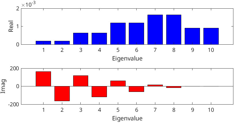
From the discussion immediately following Equation 27 one might expect that the filling time $\tau$ of the cavity is given by $1/\tau=\hat{\omega}_{1}/2Q^{\prime}_{L}$. In reality, however, it is determined by the real part of the eigenvalue that corresponds to the $\pi$-mode excitation of the cavity. In order to explore this further we display the ten eigenvalues in Figure 10. The upper plot shows the real parts of the eigenvalues and the bottom plot shows the corresponding imaginary parts, which is much larger than the corresponding real parts. We also observe that the eigenvalues come in complex-conjugate pairs; adjacent real parts have the same magnitude and the corresponding imaginary parts have opposite sign. Here a large imaginary part indicates that the mode is mostly oscillating. They are responsible for the oscillatory behavior of the cavity voltages at the start of the pulse, highlighted in Figure 5. The real parts of eigenvalues 1 and 2 are particularly small, so they cause oscillations of the corresponding mode to linger on for a relatively long time. At the same time, their imaginary part is large, such that they are oscillating substantially. This explains the excitation of the imaginary part, the Q-phase, in Figure 6. The reason that the first eight eigenvalues are excited at all comes from the sudden rise of the pulse from the generator, which contains many frequencies. And some of them are inside the bandwidth of the first four modes that are described by the first eight eigenvalues. On the other hand, the pair of eigenvalues numbered 9 and 10 show the smallest imaginary part (red) while still having a moderate real part (blue). These two modes therefore mostly absorb the energy delivered by the generator.

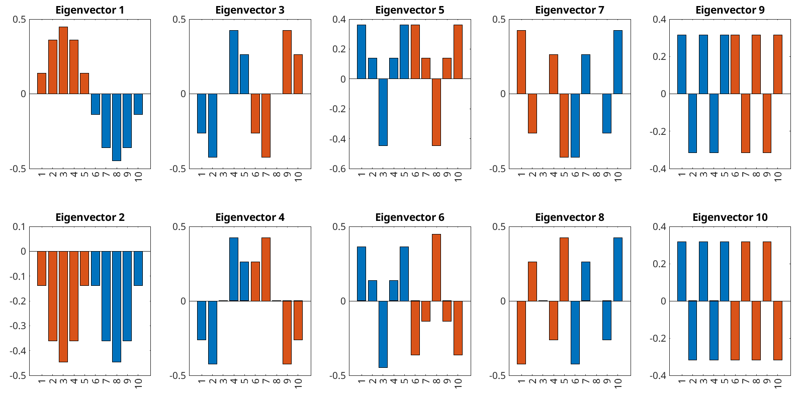
The upper row in Figure 10 shows the odd-numbered eigenvectors. The real parts are shown in blue and the imaginary parts in red. That they come in groups of five is a consequence of ordering the voltages when transforming the complex-valued Equation 31 to its real-valued counterpart Equation 45. We observe that the modal pattern follows the modes already seen in Figure 3. Only here the real (blue) and imaginary (red) parts mimic each other. The bottom row shows the complex-conjugate even-numbered eigenvectors. They show the same real part (blue) as the corresponding plot above, but the sign of the imaginary part (red) is reversed.

In particular, eigenvectors 9 and 10 display the excitation pattern of the $\pi$-mode with adjacent cells having opposite polarity. Notably, we already found that the imaginary part of the corresponding eigenvalues 9 and 10 is particularly small and therefore, rather than oscillating, this mode absorbs most of the energy from the generator. And the real part of the eigenvalues determines the filling time $\tau=1/\mathop{\mathrm{real}}(\lambda_{9})$ of the $\pi$-mode. Comparing its numerical value with $1/\tau^{\prime}=\hat{\omega}/2Q^{\prime}_{L}$ we find that $\tau=5\tau^{\prime}$. It takes five times longer to fill a five-cell cavity compared to filling a single cell. After all, we have to provide power to fill five cells rather than one, and that takes five times longer. Using a complementary point of view: the five cells behave like five bandpass filters in series and therefore the overall bandwidth is reduced five-fold.

In order to see the temporal dependence of the five modes, we create projectors onto their corresponding eigenspaces. These eigenspaces are spanned by the columns of $W$, which are the eigenvectors of $W$ from Equation 50. Therefore, we can write

$$W=\left(\ket{w_{1}},\ket{w_{2}},\dots,\ket{w_{10}}\right)\ .$$ (53)

Here we borrow the notation with bra and ket vectors from quantum mechanics, where ket denotes column vectors, the eigenvectors $\ket{w_{i}}$, $i=1,\dots,10$ that are the columns of the matrix $W$. In a similar fashion, we denote the row vectors of $W^{-1}$ by the $\bra{w_{i}}$, thus

$$W^{-1}=\left(\begin{array}[]{c}\bra{w_{1}}\\ \vdots\\ \bra{w_{10}}\end{array}\right)\ .$$ (54)

Using this notation, we can rewrite Equation 50 as a spectral decomposition

$$\tilde{A}=\sum_{i=1}^{10}\lambda_{i}P_{i}\qquad\mathrm{with}\qquad P_{i}=\ket{w_{i}}\bra{w_{i}}\ ,$$ (55)

where $P_{i}$ is the projector onto the subspace characterized by eigenvalue $\lambda_{i}$ and $\ket{w_{i}}\bra{w_{i}}$ is the outer product of column vector $\ket{w_{i}}$ and the row vector $\bra{w_{i}}$. Note that $\tilde{A}$ is not symmetric and therefore $W$ is neither real nor orthogonal. Since the eigenvalues come in complex conjugate pairs, we use the sum of $P_{1}$ and $P_{2}$ or $Q_{1}=P_{1}+P_{2}$, for example, to determine the contribution of the $\pi/5$-mode to the voltage $\tilde{V}(s)$, which is given by $V(\pi/5)=Q_{1}\tilde{V}(s)$. Building the projectors for the other modes works analogously. The upper plot in Figure 10 shows the amplitude of this mode, given by the norm of $V(\pi/5)$. We observe that it only slowly decays owing to the fact that eigenvalues $\lambda_{1}$ and $\lambda_{2}$ have the smallest real part and therefore correspond to the longest time constant, as already discussed above. All modes, except the $\pi$-mode shown on the bottom plot, decay to small values long before the generator is turned off at 3.5 ms. Only the amplitude of the $\pi$-mode increases to much larger values than the other four modes and follows the behavior already seen on the top plots in Figures 6 and 7.

Figure 11: The voltage in the single cell cavity (magenta) superimposed to the voltage in the five-cell cavity (black).

It is instructive to compare the behavior of a the five-cell cavity operating in $\pi$-mode to a single-cell cavity. In the absence of any imperfections, we describe [6] the voltage $V$ in a single-cell resonator that is driven with current $I$ by

$$\frac{dV}{dt}=-\omega_{12}V+\frac{\omega_{12}R}{1+\beta}I\qquad\mathrm{with}\qquad\omega_{12}=\frac{\hat{\omega}}{2Q_{L}}=(1+\beta)\frac{\hat{\omega}}{2Q}\ .$$ (56)

This equation straightforward to integrate such that the the voltage after starting up the generator is given by

$$V(t)=\left(1-e^{-\omega_{12}t}\right)V_{\infty}\qquad\mathrm{with}\qquad V_{\infty}=\frac{IR}{1+\beta}\ ,$$ (57)

where $V_{\infty}$ is the asymptotic steady-state voltage. After the generator has turned off, the voltage decreases exponentially $V(t)=V_{a}e^{-\omega_{12}t}$, where $V_{a}$ is the voltage immediately before the generator is turned off.

Figure 11 shows the voltage in the single-cell cavity superimposed on the voltages in cells 1, 3, and 5 of a five-cell cavity operated in $\pi$-mode. The latter was already shown in the upper plot in Figure 6. In the single-cell model, we have to increase $Q$ and thereby the time constant $1/\omega_{12}$ by a factor of five to account for filling five cells, rather than a single cell. But this leads to almost perfect agreement of the curves in Figure 11 and largely justifies the commonly-used approximation of a multi-cell cavity by a single-cell equivalent model.

After considering the perfect $\pi$-mode cavity, we now turn to the consequences of imperfections such as incorrect coupling $\kappa_{i}$ or deviations of one cell’s unloaded $Q$-value $Q_{i}$ and resonance frequency $\hat{\omega}_{i}$ from the design values.

5 Incorrect coupling $\kappa_{i}$ between cells

We now assume that the $\kappa_{i}$ possibly differ from their design value value $\kappa$ by $\Delta\kappa_{i}$. We also assume that all capacitances $C_{i}$ are equal and that leads to $\kappa^{\prime}_{j}=\kappa_{j-1}$. Furthermore, the coupling to the beam pipe can differ from the design value according to $\kappa_{a}=2\kappa+\Delta\kappa_{a}$ and $\kappa_{b}=2\kappa+\Delta\kappa_{b}$. This causes us to modify Equation 27 and 4 for the first cell as follows

$$\left(2+6\kappa+\kappa_{1}+\Delta\kappa_{a}\right)\frac{d\tilde{V}_{1}}{dt}-\kappa_{1}\frac{d\tilde{V}_{2}}{dt}$$ (58)

$$\qquad=-\frac{\hat{\omega}}{Q^{\prime}_{L}}\tilde{V}_{1}+i\frac{\hat{\omega}}{\sqrt{1+4\kappa}}\left[(2\kappa-\kappa_{1}-\Delta\kappa_{a})\tilde{V}_{1}+\kappa_{1}\tilde{V}_{2}\right]+\frac{\hat{\omega}R_{1}}{Q_{1}}\frac{\tilde{I}_{g}}{n}\ .$$

For the cells in the middle of the cavity Equations 18 and 4 are modified to

$$-\kappa_{j-1}\frac{d\tilde{V}_{j-1}}{dt}+\left(2+4\kappa+\kappa_{j-1}+\kappa_{j}\right)\frac{d\tilde{V}_{j}}{dt}-\kappa_{j}\frac{d\tilde{V}_{j+1}}{dt}$$ (59)

$$\qquad\quad=-\frac{\hat{\omega}}{Q}\tilde{V}_{j}+\frac{i\hat{\omega}}{\sqrt{1+4\kappa}}\left[\kappa_{j-1}\tilde{V}_{j-1}+\left(4\kappa-\kappa_{j-1}-\kappa_{j}\right)\tilde{V}_{j}+\kappa_{j}\tilde{V}_{j+1}\right]\ .$$

Finally Equations 23 and 4, describing the last cell $n$, become

$$-\kappa_{n-1}\frac{d\tilde{V}_{n-1}}{dt}+\left(2+6\kappa+\kappa_{n-1}+\Delta\kappa_{b}\right)\frac{d\tilde{V}_{j}}{dt}$$ (60)

$$\qquad\qquad=-\frac{\hat{\omega}}{Q}\tilde{V}_{n}+\frac{i\hat{\omega}}{\sqrt{1+4\kappa}}\left[\kappa_{n-1}\tilde{V}_{n-1}+\left(2\kappa-\kappa_{n-1}-\Delta\kappa_{b}\right)\tilde{V}_{n}\right]\ .$$

For the simulations we convert these equations to matrix-valued equations. Compared to Equation 4, only the matrices $D$ and $B$ need to be modified to

$$D = \left(\begin{array}[]{ccccc}2+6\kappa+\kappa_{1}+\Delta\kappa_{a}&-\kappa_{1}&0&0&0\\ -\kappa_{1}&2+4\kappa+\kappa_{1}+\kappa_{2}&-\kappa_{2}&0&0\\ 0&-\kappa_{2}&2+4\kappa+\kappa_{2}+\kappa_{3}&-\kappa_{3}&0\\ 0&0&-\kappa_{3}&2+4\kappa+\kappa_{3}+\kappa_{4}&-\kappa_{4}\\ 0&0&0&-\kappa_{4}&2+6\kappa+\kappa_{4}+\Delta\kappa_{b}\end{array}\right)$$ (66)

$$B = \frac{\hat{\omega}\Delta t}{\sqrt{1+4\kappa}}\left(\begin{array}[]{ccccc}2\kappa-\kappa_{1}-\Delta\kappa_{a}&\kappa_{1}&0&0&0\\ \kappa_{1}&4\kappa-\kappa_{1}-\kappa_{2}&\kappa_{2}&0&0\\ 0&\kappa_{2}&4\kappa-\kappa_{2}-\kappa_{3}&\kappa_{3}&0\\ 0&0&\kappa_{3}&4\kappa-\kappa_{3}-\kappa_{4}&\kappa_{4}\\ 0&0&0&\kappa_{4}&2\kappa-\kappa_{4}-\Delta\kappa_{b}\end{array}\right)\ .$$ (72)

It is easy to see that these expressions revert to those in Equation 4 if all $\kappa_{i}$ are equal to $\kappa$ and both $\Delta\kappa_{a}$ and $\Delta\kappa_{b}$ are zero.

Figure 12: The left plot corresponds to Figure 7, only here the coupling between the second and third cell is increased by $\Delta\kappa_{2}=2\times 10^{-6}$ from the design value of $\kappa_{2}=0.01$. The right shows the amplitude of the voltage in the fifth cell $|V_{5}|$ after 3 ms versus $\Delta\kappa_{2}$ (solid) and $\Delta\kappa_{a}$ (dotted) in the range $\pm 2\times 10^{-5}$.

The left-hand plot in Figure 12 shows the I and Q phase of the field in the fifth cell on the top and the reflected signals on the bottom. Here the coupling between the second and third cell is increased by $\Delta\kappa_{2}=2\times 10^{-6}$ compared to the situation shown in Figure 7. On the top we observe that the maximum achievable signal is substantially reduced from $2\times 10^{5}$ to $1.3\times 10^{5}$ with respect to Figure 7 and in both top and bottom plot a significant imaginary phase (Q-phase, shown in red) appears. Moreover, some ringing in the signal is visible. It turns out that the eigenvalue of the $\pi$-mode, which was purely real in the situation depicted in Figure 7, now acquires a small imaginary component, which causes the onset of an oscillation. Increasing $\Delta\kappa_{2}$ further makes the ringing very obvious, though we do not show any plots.

The solid line in the plot on the right-hand side in Figure 12 shows the amplitude of the field in the fifth cell $|V_{5}|$ as a function of $\Delta\kappa_{2}$, which displays a distinct resonance-like behavior. The full-width-at-half-maximum of the curve is $4.2\times 10^{-6}$, which may serve as a specification for the tolerance for manufacturing the cavity and especially the cell-to-cell coupling. The dotted line shows the corresponding response of varying the coupling to the beam pipe $\kappa_{a}$ by $\Delta\kappa_{a}$ in the same range. We find that the curve is about three times as wide, indicating slightly relaxed tolerances for manufacturing the cavity ends.

In the next section, we perform a comparable analysis for variations in the unloaded quality factor $Q_{i}$ of the cells.

6 Incorrect quality factor $Q_{i}$ of cells

Figure 13: The left plot corresponds to Figure 6, only here the quality factor in the fifth cell $Q_{5}$ is reduced by a factor 1000 to $10^{6}$. The plot on the right shows the voltage amplitude in the fifth cell $|V_{5}|$ after 3 ms as a function of $Q_{5}$ in the range $10^{5}$ to $10^{10}$.

Losses in the cells are modeled by varying the cell’s resistance $R_{i}$, which predominantly affects the quality factor $Q_{i}=R_{i}\sqrt{C_{i}/L_{i}}$, but also the coupling $\beta=R_{1}/n^{2}Z_{0}$ of the first cell. To account for the losses, we only have to modify the array $A$ in Equation 4 to

$$A=\mathop{\mathrm{diag}}\left((1+\beta)\frac{\hat{\omega}\Delta t}{Q_{1}},\frac{\hat{\omega}\Delta t}{Q_{2}},\frac{\hat{\omega}\Delta t}{Q_{3}},\frac{\hat{\omega}\Delta t}{Q_{4}},\frac{\hat{\omega}\Delta t}{Q_{5}}\right)$$ (73)

and leave the other quantities unaffected. The plot on the left-hand side in Figure 13 corresponds to Figure 6, which shows the unperturbed system. These figures show the I and Q-phases of the voltages in cells 1, 3, and 5 during a pulse. Only here the quality factor of the fifth cell $Q_{5}$ is reduced by a factor 1000 from $10^{9}$ to $10^{6}$. The upper graph shows the real (I-phase) part of the voltages. Here we observe a small reduction of the amplitude compared to Figure 6. The reduction of $Q_{5}$ causes the lower graph, showing the imaginary (Q-phase), to exhibit a small splitting of this phase in the three cells. We interpret this as the fifth cell absorbing most of the power that has to pass through the preceding cells and the losses are somewhat bigger than can be replenished continuously by the generator.

The plot on the right-hand side in Figure 13 shows the reduction of the absolute value of the voltage in the fifth cell $|V_{5}|$ as a function of $Q_{5}$. As long as only $Q_{5}$ is reduced and the dissipated energy does not quench neighboring cells, the voltage $|V_{5}|$ is only weakly affected, unless it is reduced below a few times $10^{6}$.

Figure 14: The field in the fifth cell $V_{5}$ and the reflected signal $V_{ref}$ while the first cell quenches after 2.5 ms. The resistance $R_{1}$ is decreased by $x=10^{3}$ on the left-hand plot and by $10^{5}$ on the right-hand plot.

Increased losses in the first cell need a little extra attention, because both $Q_{1}$ and $\beta$ are affected. Let us assume that the resistance $R_{1}$ is decreased by some factor $x$. A big quench is characterized by a large value of $x$, say $10^{5}$. This factor reduces $Q_{1}$ to $Q_{1}/x$ and $\beta$ to $\beta/x$, such that the first entry in the matrix $A$ will become $(1+\beta/x)/(Q_{1}/x)=(x+\beta)/Q_{1}$ where $Q_{1}$ and $\beta$ are the default values. Here we see that as long as $x$ is smaller than $\beta$ a quench in the first cell will only have a modest effect on the time constant of the first cell, which is the first entry in the matrix $A$.

Each of the plots in Figure 14 shows the field in the fifth cell $V_{5}$ and the reflected signal $V_{ref}$ in situations where a quench happens after 2.5 ms. In the plots on the top row the first cell quenches. We simulate it by decreasing the resistance $R_{1}$ by a factor $x=10^{3}$ (left) and $x=10^{5}$ (right). The weaker quench, shown on the left, only leads to a moderate drop of the voltage $V_{5}$, whereas the bigger quench, shown on the right, leads to an almost complete collapse of the field in the cavity and corresponding change in the reflected signal. The two plots in the bottom row correspond to quenches with equal magnitude of the fourth cell, that we model by reducing $R_{4}$. We find that the behavior of the signals $V_{5}$ and $V_{ref}$ is very similar to that shown in the top row.

Finally, let us consider what happens if one or several cells are detuned.

7 Detuned cells

In this section we assume that the resonance frequency $\hat{\omega}_{j}$ of cell $j$ deviates from the design value $\hat{\omega}$ by $\Delta\omega_{j}=\hat{\omega}_{j}-\hat{\omega}$. Moreover, for the $\pi$-mode we have $\hat{\omega}^{2}/\omega^{2}_{\pi}=1+4\kappa$ which gives us

$$\frac{\hat{\omega}^{2}_{j}}{\omega_{\pi}^{2}}=\frac{\hat{\omega}^{2}+2\hat{\omega}\Delta\omega_{j}+\Delta\omega_{j}^{2}}{\omega_{\pi}^{2}}\approx 1+4\kappa+2\frac{\Delta\omega_{j}}{\hat{\omega}}\approx 1+4\kappa+\delta_{j}$$ (74)

with the abbreviation $\delta_{j}=2\Delta\omega_{j}/\hat{\omega}$ to describe the relative detuning of cell $j$.

Assuming all other parameters to be equal their design values, the equation for the first cell becomes

$$\left(2+7\kappa+\delta_{1}\right)\frac{d\tilde{V}_{1}}{dt}-\kappa\frac{d\tilde{V}_{2}}{dt}$$

$$\qquad\qquad=-\frac{\hat{\omega}}{Q^{\prime}_{L}}\tilde{V}_{1}+i\frac{\hat{\omega}}{\sqrt{1+4\kappa}}\left[(\kappa+\delta_{1})\tilde{V}_{1}+\kappa\tilde{V}_{2}\right]+\frac{\hat{\omega}R_{1}}{Q_{1}}\frac{\tilde{I}_{g}}{n}\ .$$

For cell $j$ in the middle of the cavity we obtain

$$-\kappa\frac{d\tilde{V}_{j-1}}{dt}+\left(2+6\kappa+\delta_{j}\right)\frac{d\tilde{V}_{j}}{dt}-\kappa\frac{d\tilde{V}_{j+1}}{dt}$$ (76)

$$\qquad\qquad=-\frac{\hat{\omega}}{Q}\tilde{V}_{j}+i\frac{\hat{\omega}}{\sqrt{1+4\kappa}}\left[\kappa\tilde{V}_{j-1}+(2\kappa+\delta_{j})\tilde{V}_{j}+\kappa\tilde{V}_{j+1}\right]$$

and the equation for the last cell is

$$-\kappa\frac{d\tilde{V}_{n-1}}{dt}+\left(2+7\kappa+\delta_{n}\right)\frac{d\tilde{V}_{j}}{dt}$$ (77)

$$\qquad\qquad=-\frac{\hat{\omega}}{Q}\tilde{V}_{n}+i\frac{\hat{\omega}}{\sqrt{1+4\kappa}}\left[\kappa\tilde{V}_{n-1}+(\kappa+\delta_{n})\tilde{V}_{n}\right]\ .$$

In all equations we approximated $\hat{\omega}_{j}/Q_{j}$ by $\hat{\omega}/Q$ and thus neglected the very small effect of the detuning on damping. This leaves the matrix $A$, used in the simulations, unaffected. On the other hand, the change of a cell’s resonance frequency mainly affects the matrices $D$ and $B$

$$D = \left(\begin{array}[]{ccccc}2+7\kappa+\delta_{1}&-\kappa&0&0&0\\ -\kappa&2+6\kappa+\delta_{2}&-\kappa&0&0\\ 0&-\kappa&2+6\kappa+\delta_{3}&-\kappa&0\\ 0&0&-\kappa&2+6\kappa+\delta_{4}&-\kappa\\ 0&0&0&-\kappa&2+7\kappa+\delta_{5}\end{array}\right)$$ (83)

$$B = \frac{\hat{\omega}\Delta t}{\sqrt{1+4\kappa}}\left(\begin{array}[]{ccccc}\kappa+\delta_{1}&\kappa&0&0&0\\ \kappa&2\kappa+\delta_{2}&\kappa&0&0\\ 0&\kappa&2\kappa+\delta_{3}&\kappa&0\\ 0&0&\kappa&2\kappa+\delta_{4}&\kappa\\ 0&0&0&\kappa&\kappa+\delta_{5}\end{array}\right)\$$ (89)

which makes it straightforward to incorporate detuned cells in the simulations.

Figure 15: This figure corresponds to Figure 13, but on the left-hand plot the fourth cell is detuned by $\delta_{4}=5\times 10^{-6}$. The right-hand plot shows the voltage amplitude in the fifth cell $|V_{5}|$ plotted against the detuning $\delta$ of the fourth cell (black dashes) and if all cells are detuned by the same amount (red).

In the simulations in this section we keep all parameters at their default values, only the detuning is varied. The left-hand plot in Figure 15 shows the voltage in the fifth cell $V_{5}$ in the upper panel and the reflected signal $V_{ref}$ on the lower panel. In this simulation, the fourth cell is detuned by $\delta_{4}=5\times 10^{-6}$ which approximately corresponds to twice the loaded bandwidth $(1+\beta)/2Q$ of the cavity. We see that the real and imaginary phase of $V_{5}$ and $V_{ref}$ have similar magnitude, indicating the substantial influence of the detuning. We also observe that the amplitude of $V_{5}$ is reduced. In passing we note that detuning all cells by $\delta=10^{-6}$, which is one fifth of $\delta_{4}$, the plot of $V_{5}$ and $V_{ref}$ is virtually unchanged. In other words, from observing the transmitted $V_{5}$ and the reflected signal $V_{ref}$ we cannot tell whether one cell is detuned or all are detuned by a smaller amount. Finally, the right-hand plot in Figure 15 shows the amplitude in the fifth cell $|V_{5}|$ versus the detuning. The dashed black curve corresponds to the fourth cell detuned and the red curve corresponds to all cells detuned by the same amount $\delta$. We see that the red curve is much narrower than the black one, indicating the much higher sensitivity when detuning all cells, compared to detuning only a single cell.

8 Conclusions

We found that multi-cell cavities behave very similar to single-cell cavities, as is witnessed by the close agreement of the two curves in Figure 11. The reason is that it takes only on the order of microseconds for the $\pi$-mode to form, which is shown in Figure 5. The other modes are excited but they do not absorb power to build up a coherent mode. Instead, they damp away as shown in the upper four plots in Figure 10, where the individual time constants are related to the real part of the eigenvalues shown in Figure 10. Basically, apart from short-lived transients of the other modes, the $\pi$-mode dominates the dynamics of the electro-magnetic fields in multi-cell cavities and oscillates as an entity, rather than the weakly-coupled fields in the cells oscillating independently.

That the $\pi$-mode oscillates as an entity has ramifications for the tolerances to which the cells must be manufactured, because the $\pi$-mode averages over the contributions of the individual imperfections. We determined the tolerance with respect to the cell-to-cell coupling $\kappa$ and show the result on the right-hand plot in Figure 12, which shows a resonance-like curve whose width determines the sensitivity with respect to $\kappa$. Furthermore, the right-hand plot in Figure 15 shows the sensitivity with respect to detuning of individual cells, which is more relaxed than detuning all cells by the same amount. In Figure 14 we found that a quench in a single cell can be stabilized if it is “small” in the sense that the losses are comparable to the losses that escape through the input coupler, which is given by $\beta$. If the reduction $x=Q/Q_{quench}\gg\beta$ of one cell, the quench leads to a collapse of the $\pi$-mode as shown on the right-hand plots in Figure 14.

The methods developed for this report can be easily extended to other cavities and can then be used to estimate manufacturing tolerances for a number of imperfections, such as evenness of $Q$-values or statistically distributed couplings $\kappa$ or detuning $\delta=2\Delta\omega/\hat{\omega}$.

Of particular interest are the initial high-frequency oscillations shown in Figure 5. Measuring them experimentally with a high-speed data-acquisition system and theoretically determining how they are related to cavity imperfections using methods developed for measuring $Q_{0}$ [7] seems to be a worthwhile enterprise.

This work was produced in part by Jefferson Science Associates, LLC under Contract No. AC05-06OR23177 with the U.S. Department of Energy. Publisher acknowledges the U.S. Government license and provide public access under the DOE Public Access Plan (http://energy.gov/downloads/doe-public-access-plan).

References

- [1] T. Schilcher, Vector sum control of pulsed accelerating fields in lorentz force detuned superconducting cavities, Dissertation, Universität Hamburg, 1998.
- [2] V. Ziemann, Simulations of real-time system identification of superconducting cavities with a recursive least-squares algorithm, Physical Review Accelerators and Beams 26 (2023) 112003.
- [3] H. Padamsee, J. Knobloch, T. Hays, RF Superconductivity for Accelerators, 2nd ed., Wiley-VCH, Weinheim, 2008.
- [4] M. Liepe, Superconducting Multicell Cavities for Linear Colliders, Dissertation, Universität Hamburg, 2001.
- [5] T. Powers, N. Brock, T. Ganey In Situ Plasma Processing of Superconducting Cavities at JLab, 2023 Update, Proceedings of the 21st International Conference on RF Superconductivity SRF2023 (2023) 701.
- [6] V. Ziemann, Hands-On Accelerator Physics Using MATLAB, 2nd ed., CRC Press, Boca Raton, 2025.
- [7] V. Ziemann, A new method to measure the unloaded quality factor of superconducting cavities, Physical Review Accelerators and Beams 27 (2024) 032001;